Bayesian nonparametric mixtures of Archimedean copulas

Abstract

Copula-based dependence modelling often relies on parametric formulations. This is mathematically convenient but can be statistically inefficient if the parametric families are not suitable for the data and model in focus. To improve the flexibility in modeling dependence, we consider a Bayesian nonparametric mixture model of Archimedean copulas which can capture complex dependence patterns and can be extended to arbitrary dimensions. In particular we use the Poisson-Dirichlet process as mixing distribution over the single parameter of the Archimedean copulas. Properties of the mixture model are studied for the main Archimedenan families and posterior distributions are sampled via their full conditional distributions. Performance of the model is via numerical experiments involving simulated and real data.

Keywords: Archimedean copula, Bayesian nonparametrics, mixture model, multivariate dependent model.

1 Introduction

Let ${\bf X}=(X_{1},X_{2},\ldots,X_{p})$ be an $p-$variate continuous random vector with joint cumulative distribution function (CDF) $F(x_{1},\ldots,x_{p})$ and marginal CDFs $F_{j}(x)$ for $j=1,\ldots,p$. Following Sklar, (1959), there exists a unique multivariate copula function $C(u_{1},\ldots,u_{p})$ with $C:[0,1]^{p}\to[0,1]$ that satisfies the conditions to be a proper CDF with uniform marginals, such that $F(x_{1},\ldots,x_{p})=C(F_{1}(x_{1}),\ldots,F_{p}(x_{p}))$.

Dependence or association measures between any two random variables $(X_{j},X_{k})$, independently of their marginal distributions, can be entirely written in terms of the Copula. For instance Kendall’s $\tau$ between the $j$-th and $k$-th components of ${\bf X}$ is defined as $\tau=4\mbox{E}\{C_{jk}(U_{j},U_{k})\}-1$, in other words,

$$\tau=4\int_{0}^{1}\int_{0}^{1}C_{jk}(u_{j},u_{k})f_{jk}(u_{j},u_{k})\mbox{d}u_{j}\mbox{d}u_{k}-1$$ (1)

where $C_{jk}$ is the marginal bivariate copula of $(U_{j},U_{k})$ and $f_{jk}$ is the corresponding bivariate density (e.g. Nelsen,, 2006). Clearly, flexible models for the copula are beneficial because they capture complex dependence patterns and can return accurate estimates for dependence measures of interest.

Copulas are often modeled in statistical applications using parametric families such as those included in the large class of Arhimedean copulas (e.g. Nelsen,, 2006). A Bayesian semiparametric version of an Archimedean copula was introduced by Hoyos-Argüelles and Nieto-Barajas, (2020). Nonparametric copulas are, for example, the empirical copula (Deheuvels,, 1979), the sample copula (González-Barrios and Hoyos-Argüelles,, 2018) and a Bayesian counterpart of the sample copula (Nieto-Barajas and Hoyos-Argüelles,, 2024).

Bayesian nonparametric models for multivariate data usually rely on mixtures of a multivariate normal density mixing over the mean vector and/or the covariance matrix via a Bayesian nonparametric model. In particular, Carmona et al., (2019) used a location mixture of multivariate normals for the clustering of mixed scale data, and Kottas et al., (2005) use a location-scale mixture of multivariate normals for modelling multivariate ordinal data.

In this paper we consider Bayesian nonparametric mixtures of Archimedean copulas in which the mixing distribution is the two parameter generalisation of the Dirichlet process, called Poisson-Dirichlet process, introduced by Pitman and Yor, (1997). This extension is directed towards two important goals. First, it extends considerably the range of dependence patterns that can be modeled using Archimedean copulas, making it useful for capturing complex dependencies. Second, in the case of heterogeneous populations, it clusters the sample based on information contained in the marginals, and the dependence structure. Those familiar with Bayesian nonparametric models with Gaussian distributions (e.g. Müller et al.,, 1996) will recognize that our model is a generalization, since the Archimedean copulas can accommodate different marginals and will have different tail behaviour from that of a bivariate Gaussian distribution, e.g. they are asymmetric.

The contents of the rest of the paper is as follows: In Section 2 we introduce notation and briefly review the family of Archimedean copulas and characterise it by the copula density required in the mixture model. Section 3 presents the mixture model, a study of its properties and a guide for sampling the posterior. In Section 4 we investigate the performance of our model via numerical experiments. The paper ends with conclusions and future directions for research.

2 Archimedean copula densities

To proceed, we must first introduce some notation. Let $\mbox{Un}(\alpha,\beta)$ denote a uniform density in the continuous interval $(\alpha,\beta)$; $\mbox{Ga}(\alpha,\beta)$ denote a gamma density with mean $\alpha/\beta$; $\mbox{Be}(\alpha,\beta)$ denotes a beta density with mean $\alpha/(\alpha+\beta)$; $\mbox{N}(\mu,\lambda)$ denotes a normal density with mean $\mu$ and precision $\lambda$. The density evaluated at a specific point $x$, will be denoted, for instance for the gamma case, as $\mbox{Ga}(x\mid\alpha,\beta)$.

As mentioned above, a $p$-dimensional copula $C$ is a multivariate cumulative distribution function (CDF) with uniform marginals. One of the richest class of copulas is the so-called Archimedean family. This family is defined by a continuous, decreasing and convex generator function $\phi$ such that $\phi:[0,1]\to\mathbb{R}^{+}$, $\phi(0)=\infty$, $\phi(1)=0$. Specifically, the copula with generator $\phi$ is defined as

$$C(u_{1},\ldots,u_{p})=\phi^{-1}\{\phi(u_{1})+\cdots+\phi(u_{p})\}.$$ (2)

According to McNeil and Nes̃lehová, (2009), an Archimedean copula $C$ admits a density $f_{C}$ if and only if the $(p-1)$th derivative of $\phi^{-1}$, denoted as $\phi^{-1(p-1)}$, exists and is absolutely continuous on $(0,\infty)$. In this case, the density is given by

$$f_{C}(u_{1},\ldots,u_{p})=\phi^{-1(p)}\left\{\sum_{j=1}^{p}\phi(u_{j})\right\}\prod_{j=1}^{p}\phi^{(1)}(u_{j}),$$ (3)

where $\phi^{(1)}$ denotes the first derivative of $\phi$. If all derivatives , $\phi^{-1(j)}$ of $\phi^{-1}$, exist, they must satisfy

$$(-1)^{j}\phi^{-1(j)}(u)\geq 0,$$

for $j=1,\ldots,p$. In such a case it is said that $\phi^{-1}$ is completely monotonic (Wu et al.,, 2007).

Using the relationship between derivatives of inverse functions, the copula density, for $p=2$, can be written in terms of derivatives of the generator as

$$f_{C}(u_{1},u_{2})=-\frac{\phi^{(1)}(u_{1})\phi^{(1)}(u_{2})\phi^{(2)}\{C(u_{1},u_{2})\}}{\left[\phi^{(1)}\{C(u_{1},u_{2})\}\right]^{3}},$$ (4)

where $C(u_{1},u_{2})$ is given in (2)and $\phi^{(j)}$ is the $j$-th derivative of $\phi$.

Generators $\phi$ usually belong to parametric families parametrised in terms of a single parameter $\theta$ that takes values in a parameter space $\Theta$. Therefore, we will use the notation $\phi_{\theta}(t)$ for the parametric generator and $C({\bf u}\mid\theta)$ for the copula. We consider here five widely used members of the Archimedean family: Ali–Mikhail–Haq (AMH), Clayton (CLA), Frank (FRA), Gumbel (GUM) and Joe (JOE). Generators associated to each of these families are given in Table 1, together with their parameter space and Kendall’s tau. First and second derivatives of the generators $\phi_{\theta}(t)$, required to compute bivariate copula densities, as in (4), are given in Table 2.

One way to assess the difference in the dependence induced by these five Archimedean copula families, is by studying their corresponding Kendall’s tau. In Figure 1 we plot $\tau_{\theta}$ as a function of $\theta\in\Theta$. Out of the five copula families considered, in the case of the Clayton, Frank and Joe classes, the Kendall’s tau association coefficient spans the whole range $(-1,1)$ as the copula parameter varies over its domain. The other two members induce only constrained associations, with $\tau\in[-0.1817,1/3]$ for the AMH and $\tau\in[0,1)$ for the Gumbel.

To define Archimedean copulas of dimension larger that two, we have to be careful when identifying the parameter space. To be specific, let us consider a setting with $p=3$ variables. Assume that $U_{1}$ and $U_{2}$ have positive dependence and $U_{1}$ and $U_{3}$ have negative dependence, therefore $U_{2}$ and $U_{3}$ must have negative dependence. Since dependence in Archimedean copulas is determined by a single parameter $\theta$, the previous three variables setting may not occur in a three-dimensional Archimedean copula. Variables in an Archimedean copulas are exchangeable, so the dependence between any pair of variables has to be too. This feature is preserved by the mixture setting we are proposing. However, the advantage provided by our construction is that it can model heterogeneity in the dependence structure across the population. This flexibility is accompanied by the ability to cluster bivariate data according to information contained by marginals and the copula.

To avoid the previous problems, the authors that study Archimedean copulas for $p>2$ usually constrain the parameter space $\Theta$ to their positive values. See, for example, Hofert et al., (2012), who also present analytical derivatives of order $p$ of the inverse generators $\phi_{\theta}^{-1}(t)$ for families in Table 1, for the positive values of the parameter space $\Theta$.

3 BNP mixtures

3.1 Model

Although Archimedean copulas are easy to generalise for multivariate data, the dependence might be too restrictive, since it depends only on a single parameter $\theta$. To equip the model with extra flexibility, we propose to mix the Archimedean copulas via a Bayesian nonparametric prior.

In particular, we choose the two-parameter extension of the Dirichlet process introduced by Pitman and Yor, (1997). This Poisson-Dirichlet process is almost surely (a.s.) discrete, admits a stick-breaking construction, and can be marginalised to simplify the implementation (Ishwaran and James,, 2001). A probability measure $G$ has a Poisson-Dirichlet prior with scalar parameters $a\in[0,1)$, $b>-a$ and mean parameter $G_{0}$, denoted as $G\sim\mbox{PD}(a,b,G_{0})$, when

$$G(\cdot)=\sum_{k=1}^{\infty}\omega_{k}\delta_{\theta_{k}}(\cdot),$$ (5)

where $\omega_{1}=\nu_{1}$ and $\omega_{k}=\nu_{k}\prod_{j<k}(1-\nu_{j})$ for $k=2,3\ldots$, with $\nu_{k}\stackrel{{\scriptstyle\mbox{\scriptsize{ind}}}}{{\sim}}\mbox{Be}(1-a,b+ka)$, and independent of the weights, locations $\theta_{k}\stackrel{{\scriptstyle\mbox{\scriptsize{iid}}}}{{\sim}}G_{0}$ for $k=1,2,\ldots$, and $\delta_{\theta}$ is a point mass at $\theta$. The functional parameter $G_{0}$ is known as centering measure since $\mbox{E}(G)=G_{0}$. There are two particular cases that can be obtained with the Poisson-Dirichlet prior, the Dirichlet process when $a=0$ and the normalized stable process when $b=0$.

A Bayesian nonparametric mixture model can be defined by mixing parametric Archimedean copulas $C({\bf u}\mid\theta)$ and using the Poisson-Dirichlet process as mixing distribution for the parameter $\theta$, that is,

$$C({\bf u})=\int C({\bf u}\mid\theta)G(\mbox{d}\theta)=\sum_{k=1}^{\infty}\omega_{k}C({\bf u}\mid\theta_{k}),$$ (6)

where the last equality is obtained by considering expression (5).

The Bayesian nonparametric mixture copula model can also be defined hierarchically as follows. For $i=1,\ldots,n$

$$(U_{1i},\ldots,U_{pi})\mid\theta_{i} \stackrel{{\scriptstyle\mbox{\scriptsize{ind}}}}{{\sim}}f_{C}({\bf u}_{i}\mid\theta_{i})$$

$$\theta_{i}\mid G \stackrel{{\scriptstyle\mbox{\scriptsize{iid}}}}{{\sim}}G$$ (7)

$$G \sim\mbox{PD}(a,b,G_{0}),$$

where $f_{C}$ is given in (3). For each observed multivariate vector ${\bf U}_{i}=(U_{1i},\ldots,U_{pi})$, we assign a potentially different parameter $\theta_{i}$. However, since the Bayesian nonparametric prior is a.s. discrete, there could be ties such that $\mbox{P}(\theta_{i}=\theta_{j})>0$. This implies that the number of different $\boldsymbol{\theta}_{i}$’s is lower than $n$. Smaller values of $a$ and $b$ produce more ties.

For the centering measure $G_{0}$ we consider appropriate densities with support in the parameter space $\Theta$. In general, we denote by $g_{0}(\theta)$ the density function associated to measure $G_{0}$. In particular, we take $g_{0}(\theta)=\mbox{Un}(\theta\mid-1,1)$ for the AMH; $g_{0}(\theta)=\mbox{Ga}(\theta-k\mid c_{\theta},d_{\theta})$ for Clayton and Joe, with $k=-1$ and $k=0.238734$, respectively; $g_{0}(\theta)=\mbox{N}(\theta\mid\mu_{\theta},\lambda_{\theta})$ for Frank; and $g_{0}(\theta)=\mbox{Ga}(\theta-1\mid c_{\theta},d_{\theta})$ for the Gumbel. These choices of centering measures do not have strong impact on posterior inference since, according to Goshal et al., (1999), nonparametric mixtures have full support.

Since the $\theta_{i}$’s are conditionally independent given $G$, and $\mbox{E}(G)=G_{0}$, then a priori the parameters $\theta_{i}$ are exchangeable with marginal distribution $\theta_{i}\sim G_{0}$ for $i=1,2,\ldots,n$. In particular, Pitman, (1995) showed that if we integrate out the nonparametric measure $G$, the joint distribution of the $\theta_{i}$’s is characterized by a generalized Polya urn mechanism with conditional distribution that depends on the density $g_{0}$ of $G_{0}$ as

$$f(\theta_{i}\mid\boldsymbol{\theta}_{-i})=\frac{b+am_{i}}{b+n-1}g_{0}(\theta_{i})+\sum_{j=1}^{m_{i}}\frac{n_{i,j}^{*}-a}{b+n-1}\delta_{\theta_{i,j}^{*}}(\theta_{i}),$$ (8)

for $i=1,\ldots,n$ with $\theta_{-i}$ is the set of all $\theta_{i}$’s excluding the $i$th element and $(\theta_{i,1}^{*},\ldots,\theta_{i,m_{i}}^{*})$ denote the distinct values in $\boldsymbol{\theta}_{-i}$, each with frequencies $n_{i,j}^{*}$, $j=1,\ldots,m_{i}$. One can immediately see the importance of having $G_{0}$’s support coincide with $\Theta$.

It is not difficult to prove that association coefficients like the Kendall’s tau for a mixture copula turn out to be the mixture of the individual coefficients. In particular, the Kendall’s tau for the Bayesian nonparametric mixture model (7) is

$$\tau =4\mbox{E}\{C_{2}(U_{j},U_{k})\}-1=4\sum_{k=1}^{\infty}\omega_{k}\mbox{E}\{C_{2}(U_{j},U_{k}\mid\theta_{k})\}-1$$

$$=\sum_{k=1}^{\infty}\omega_{k}\left[4\mbox{E}\{C_{2}(U_{j},U_{k},\mid\theta_{k})\}-1\right]=\sum_{k=1}^{\infty}\omega_{k}\tau_{\theta_{k}},$$ (9)

where $\tau_{\theta_{k}}$ is the individual Kendall’s tau for each of the mixture copula components $C_{2}({\bf u}\mid\theta_{k})$. For the five Archimedean families discussed earlier, values for $\tau_{\theta}$ in terms of $\theta$ are given in Table 1.

3.2 Posterior distributions

The posterior conditional distributions for each $\theta_{i}$ are given by

$$f(\theta_{i}\mid{\bf u},\boldsymbol{\theta}_{-i})\propto(b+am_{i})f({\bf u}_{i}\mid\theta_{i})g_{0}(\theta_{i})+\sum_{j=1}^{m_{i}}(n_{i,j}^{*}-a)f_{C}({\bf u}_{i}\mid\theta_{i})\delta_{\theta_{i,j}^{*}}(\theta_{i}),$$

for $i=1,\ldots,n$.

Since the likelihood $f({\bf u}_{i}\mid\theta_{i})$ does not admit a conjugate prior $g_{0}(\theta_{i})$, we need to use an MCMC sampler to draw from these posterior conditional distributions. We use a Gibbs sampler (Smith and Roberts,, 1993), and we rely on Radford Neal’s Algorithm 8 in Neal, (2000). Specifically, we initialise the algorithm by defining $\theta_{i}$ values, for $i=1,\ldots,n$, from the prior $g_{0}$. Then the algorithm proceeds as follows:

1. For each $i=1,\ldots,n$, sample $r$ auxiliary values $\boldsymbol{\theta}^{\star}=\{\theta_{m_{i}+1}^{\star},\ldots,\theta_{m_{i}+r}^{\star}\}$ from $g_{0}$.

2. Draw $\theta_{i}$, $i=1,\ldots,n$, from

   $$f(\theta_{i}\mid{\bf u},{\bf v},\boldsymbol{\theta}_{-i},\boldsymbol{\theta}^{\star})=$$

   $$\hskip 14.22636pt\frac{1}{k_{i}}\left[\sum_{j=1}^{m_{i}}\{n_{i,j}^{*}-a\}f_{C}({\bf u}_{i}\mid\theta_{i,j}^{*})\delta_{\theta_{i,j}^{*}}(\theta_{i})+\sum_{j=m_{i}+1}^{m_{i}+r}\{(b+am_{i})/r\}f_{C}({\bf u}_{i}\mid\theta_{j}^{\star})\delta_{\theta_{j}^{\star}}(\theta_{i})\right],$$

   where $k_{i}=\sum_{j=1}^{m_{i}}\{n_{i,j}^{*}-a\}f_{C}({\bf u}_{i}\mid\theta_{i,j}^{*})+\sum_{j=m_{i}+1}^{m_{i}+r}\{(b+am_{i})/r\}f_{C}({\bf u}_{i}\mid\theta_{j}^{\star})$.

3. Compute the unique values $(\theta_{1}^{*},\ldots,\theta_{m}^{*})$ in $\boldsymbol{\theta}$ and re-sample each $\theta_{j}^{*}$, $j=1,\ldots,m$ from

   $$f(\theta_{j}\mid c.c.)\propto g_{0}(\theta_{j})\prod_{\{i:\theta_{i}=\theta_{j}^{*}\}}f_{C}({\bf u}_{i}\mid\theta_{j}),$$

   where $c.c.$ stands for clustering configuration. We suggest to perform this sampling using a random walk Metropolis-Hastings (MH) step (e.g. Robert and Casella,, 2010) as follows. Sample $\theta_{j}$ from

   $$h(\theta_{j}\mid\theta_{j}^{*})=\mbox{Un}(\theta_{j}\mid\theta_{j}^{*}-\kappa_{\theta},\theta_{j}^{*}+\kappa_{\theta})$$

   constrained to the parameter space $\theta_{j}\in\Theta$, and accept it with probability $\min\{1,f(\theta_{j}\mid c.c.)/f(\theta_{j}^{*}\mid c.c.)\}$.

The hyper parameters $(a,b)$ are crucial in determining the number of components in the mixture (7). Instead of giving them a fixed value, we can assign a hyper prior distribution. Considering the parameter space $a\in[0,1)$ and $b\in(-a,\infty)$, the joint prior would be factorised as $f(a,b)=f(b\mid a)f(a)$, where specifically, $b$ given $a$ has a shifted gamma and $a$ has a marginal beta distribution on the unit interval. In other words,

$$f(a,b)=\mbox{Ga}(b+a\mid c_{b},d_{b})\mbox{Be}(a\mid c_{a},d_{a}).$$

This prior distribution for $(a,b)$ is updated with the exchangeable partition probability function (EPPF) induced by the Poisson-Dirichlet process. This was obtained by Pitman, (1995) and is given by

$$f(n_{1}^{*},\ldots,n_{m}^{*}\mid a,b)=\frac{\Gamma(b+1)}{\Gamma(b+n)}\left\{\prod_{j=1}^{m-1}(b+ja)\right\}\left\{\prod_{j=1}^{m}\frac{\Gamma(n_{j}^{*}-a)}{\Gamma(1-a)}\right\}.$$

The Gibbs sampler is extended to include simulations from the following two conditional distributions.

1. Sample $a$ from

   $$f(a\mid b,\mbox{data})\propto\left\{\prod_{j=1}^{m-1}(b+ja)\right\}\left\{\prod_{j=1}^{m}\frac{\Gamma(n_{j}^{*}-a)}{\Gamma(1-a)}\right\}\mbox{Ga}(b+a\mid c_{b},d_{b})\mbox{Be}(a\mid p_{a},q_{a})$$

   by implementing a MH step with a random walk proposal. At iteration $(t+1)$ sample $a\sim\mbox{Un}(\max\{0,a^{(t)}-\kappa_{a}\},\min\{a^{(t)}+\kappa_{a},1\})$ and accept it with probability $\min\{1,f(a\mid b,\mbox{data})/f(a^{(t)}\mid b,\mbox{data})\}$.

2. Sample $b$ from

   $$f(b\mid a,\mbox{data})\propto\frac{\Gamma(b+1)}{\Gamma(b+n)}\left\{\prod_{j=1}^{m-1}(b+ja)\right\}\mbox{Ga}(b+a\mid c_{b},d_{b})$$

   by implementing a MH step with a random walk proposal. At iteration $(t+1)$ sample $b\sim\mbox{Ga}(\kappa_{b},\kappa_{b}/b^{(t)})$ and accept it with probability $\min\{1,f(b\mid a,\mbox{data})\mbox{Ga}(b^{(t)}\mid\kappa_{b},\kappa_{b}/b)/f(b^{(t)}\mid a,\mbox{data})/\mbox{Ga}(b\mid\kappa_{b},\kappa_{b}/b^{(t)})\}$.

The algorithm continues iterating steps (i)–(v) until convergence.

Parameters $\kappa_{\theta}$, $\kappa_{a}$ and $\kappa_{b}$ are tuning parameters that control the acceptance probability in the MH steps. Instead of fixing them, we adapt them every 50-th iteration to achieve a target acceptance rate. We aim for an acceptance probability in the interval $[0.3,0.4]$ which, according to Robert and Casella, (2010), contains the optimal value. Specifically, we use batches of 50 iterations and for every batch $j$, we compute the acceptance rate for each of the parameters $\theta_{j}^{*}$, $a$ and $b$, say $AR^{(j)}$. Then for $\kappa_{\theta}$, increase $\kappa^{(j+1)}=\kappa^{(j)}1.01^{\sqrt{j}}$ if $AR^{(j)}>0.4$ and decrease $\kappa^{(j+1)}=\kappa^{(j)}1.01^{-\sqrt{j}}$ if $AR^{(j)}<0.3$. For the other two $\kappa_{a}$ and $\kappa_{b}$, increase $\kappa^{(j+1)}=\kappa^{(j)}e^{\sqrt{j}}$ if $AR^{(j)}<0.3$ and decrease $\kappa^{(j+1)}=\kappa^{(j)}e^{-\sqrt{j}}$ if $AR^{(j)}>0.4$. We use $\kappa_{\theta}^{(1)}=0.1$, $\kappa_{a}^{(1)}=1$ and $\kappa_{b}^{(1)}=1$ as starting values.

3.3 Goodness of fit measure and predictive density

We assess the model fit by computing the logarithm of the pseudo marginal likelihood (LPML), which is a predictive measure for model performance and defined as $LPML=\sum_{i=1}^{n}\log(CPO_{i})$. The conditional predictive ordinate (CPO) statistic (Geisser and Eddy,, 1979) is defined as the predictive density for $i$-th observation given the remaining data, that is $f({\bf u}_{i}\mid{\bf u}_{-i})$. It is well known (e.g. Nieto-Barajas and Contreras-Cristán,, 2014) that the $CPO_{i}$ can be estimated with a Monte Carlo sample $\theta_{i}^{(l)}$ for $l=1,\ldots,L$ as

$$\widehat{CPO}_{i}=\left[\frac{1}{L}\sum_{l=1}^{L}\frac{1}{f_{C}({\bf u}_{i}\mid\theta_{i}^{(l)})}\right]^{-1}.$$

Kendall’s tau (9) is approximated using

$$\widehat{\tau}=\frac{1}{L}\sum_{l=1}^{L}\tau_{\theta_{0}^{(l)}},$$

and can be used to summarize the dependence in the data.

One feature of the Poisson-Dirichlet process mixture models is that the number of mixture components is automatically chosen by a data-driven process. Specifically, the number of components is given by the number of distinct parameters $m$, which can be obtained using the MCMC sample. If we wanted to estimate the number of components, we can use a zero-one loss function and report the mode, however there are multiple cluster configurations with the same number of components defined by the mode. In order to select a single clustering configuration, and produce further inferences, we propose to do a search based on the following steps:

1. Find the posterior mode of $m$, say $\widehat{m}$.

2. Define the search set as $SS=\{\widehat{m}-2,\widehat{m}-1,\widehat{m},\widehat{m}+1,\widehat{m}+2\}$. If the mode lies at the boundary of the support go up to $\widehat{m}+4$ if the mode is at the lower limit, and start from $\widehat{m}-4$ if the mode is at the upper limit.

3. Considering only iterations whose number of components $m$ belongs to the search set $SS$, form the pairwise clustering matrix $\mathbb{M}$ as the relative frequency of iterations such that individuals $\theta_{i}=\theta_{j}$, for $i\neq j\in\{1,\ldots,n\}$.

4. Follow Dahl, (2006)’s approach to select a single clustering configuration as the iteration that minimises the squared deviations with respect to the pairwise clustering matrix $\mathbb{M}$. That is, minimise the sum of the element-wise square distances. Denote the number of components obtained as $\tilde{m}$.

5. Conditional on the chosen clustering configuration, perform a post MCMC sampling of the unique parameter values $(\theta_{1}^{*},\ldots,\theta_{\tilde{m}}^{*})$ as in (iii).

With the last step of the previous procedure we can also estimate the copula parameters $\theta_{j}^{*}$ for the number of components selected $\tilde{m}$. Additionally, we can also compute the weight assigned by the model to each of the mixture components. In particular we compute the posterior mean of $(n_{j}^{*}-a)/(b+n)$, with respect to the posterior distribution of $(a,b)$, where $n_{j}^{*}$ is the number of data points assigned to cluster $j$, for $j=1,\ldots,\tilde{m}$.

4 Numerical Experiments

4.1 Bivariate simulation study

We first test our posterior inferential procedure by generating random bivariate data from two component mixtures of each of the five common Archimedean copulas from Table 1, that is, $f({\bf u})=\pi f_{C}({\bf u}\mid\vartheta_{1})+(1-\pi)f_{C}({\bf u}\mid\vartheta_{2})$. We took $\pi_{1}=1/2$ in all cases and the copula densities $f_{C}$ were specified by parameter values $(\vartheta_{1},\vartheta_{2})$ for each family as: $(-0.8,0.8)$ for AMH, $(-0.5,10)$ for the Clayton, $(-5,5)$ for the Frank, $(2,10)$ for the Joe, and $(5,10)$ for the Gumbel. We took two sample sizes to compare, $n=200$ and $n=500$. For each generated data we fitted our Bayesian nonparametric Archimedean copula mixture model using each of the five Archimedean family members as mixture densities. This leads to a total of 25 model fits.

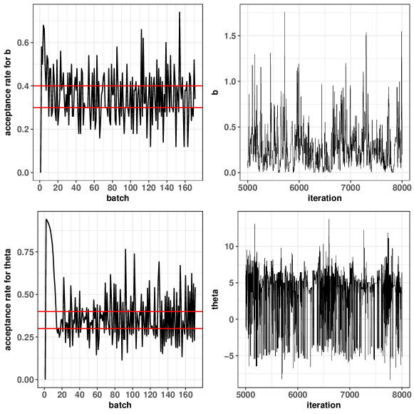
Figure 2: Acceptance rate and trace plot for $b$ (top) and $\theta$ (bottom) when the data are sampled from Frank copula and the fitted model using Frank kernel.

Our model is fully specified by determining the centering measure $g_{0}(\theta)$ and a hyper-prior for the parameters $a$ and $b$. In particular for the centering measure we took: $c_{\theta}=d_{\theta}=0.01$ for the Clayton and Joe, $\mu_{\theta}=0$ and $\lambda_{\theta}=0.1$ for the Frank, and $c_{\theta}=d_{\theta}=0.01$ for the Gumbel. For the precision parameters we took slightly informative priors to induce a small number of components: $p_{a}=1$, $q_{a}=5$, $c_{b}=1$ and $d_{b}=10$. MCMC was run for 10,000 iterations with a burn-in of 5,000. We monitor the acceptance rate for each batch, in the adaptive algorithm, and diagnose the convergence of MCMC by trace plots as shown in Figure 2.

To assess model fit we computed the LPML goodness of fit (gof) statistic defined in Section 3.3. The 25 values are reported in Tables 3 and 4 for both sample sizes, $n=200,500$, respectively. The way to read these tables is row-wise, where the largest value for each row determines the best fit. No much difference is recorded between the two sample sizes. The best model for four of the five families is obtained when we select the copula density used to generate the data. The exception is the AMH family, where the best fits are obtained by the Joe kernel. However, the second best is obtained by the AMH itself. This is because the bivariate copula from the AMH family does not yield a strong dependence, in fact, the parameters chosen induce a Kendall’s tau of $-0.099$ and $0.128$ for each of the two mixture components, respectively.

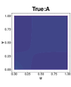
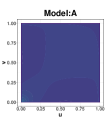
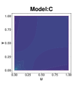
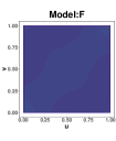
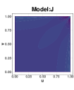
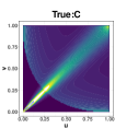
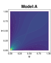
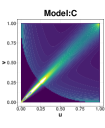
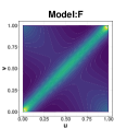
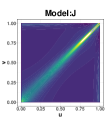
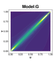
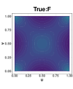
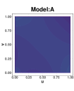
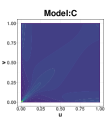
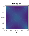
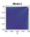
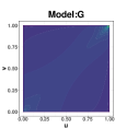
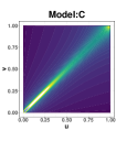
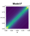
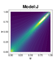
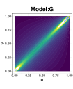
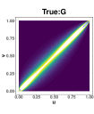
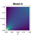
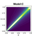
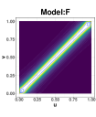
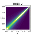
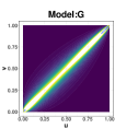
Figure 3: Density estimations for simulated bivariate data with $n=500$. Across columns: True density (1st), AMH fitting (2nd), Clayton fitting (3rd), Frank fitting (4th), Joe fitting (5th), and Gumbel fitting (6th). Data generated model across rows: AMH (1st), Calyton (2nd), Frank (3rd), Joe (4th) and Gumbel (5th).

In Figure 3 we present contour plots of the bivariate densities as heatmaps for the true model (first column) as well as the 25 fits, columns two to six. The first row contains data generated from the AMH copula. Contours from the true model do not show much difference in colour due to the weak dependence. Fitting models AMH and Clayton show similar contour patterns compared to the true one, whereas the fit based on the Joe kernel looks very dissimilar. Considering data from the mixture of Clayton copulas (second row), contours show a lower left strong positive dependence, combined with circular contours associated to negative dependence obtained by the Clayton component with negative parameter. None of models, apart form the Clayton, do a good job in capturing the true dependence.

When the data is coming from a mixture of Frank copulas (third row in Figure 3), contours of the true density show a cross pattern in the corners. The fitting obtained with the Frank kernel is the only one that replicates the shapes of the contours. In the fourth row we have the contours from a mixture of Joe copulas and it shows a strong right-upper dependence. Only models based on the Joe and Gumbel seem to capture it. Finally, when data is coming from a mixture of Gumbel copulas, apart from the Gumbel itself, the Clayton and Joe models seem to do a reasonable job.

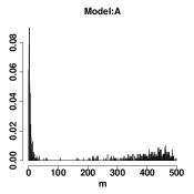
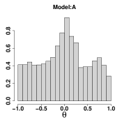
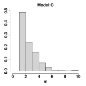
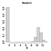
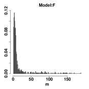
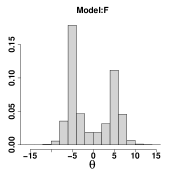
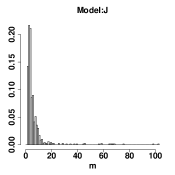
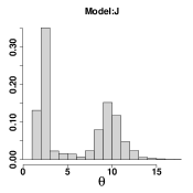
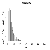
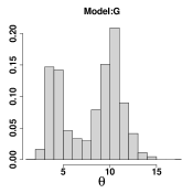
Figure 4: Simulated bivariate data with $n=500$. Posterior distributions when using the same kernel used to sample the data: the number of mixture components (1st column) and model parameters (2nd column). Models across rows: AMH (1st), Clayton (2nd), Frank (3rd), Joe (4th), and Gumbel (5th).

One feature of the Poisson-Dirichlet process mixture models is that we can assess the number of mixture components required to fit the data. Posterior distribution for the number of components with $n=500$ when using the same kernel as the one used to sample the data is presented in the first column of Figure 4. Additionally, in the second column of the same figure we present the histogram for all mixture components parameters $\theta_{i}$ combined.

For the AMH case, the posterior distribution of the number of components has a bimodal distribution, with one heavier mode at 3 and a lighter second mode at around 500. On the other hand, the posterior of the parameters shows a mode around zero with very heavy tails towards $-1$ and $1$. We recall that the true parameter values were $(-0.8,0.8)$. Since the dependence induced by the AMH copula is very weak, the model is not able to detect either the correct number of components nor the true values of the parameters. However the density estimation is very good but with a lot more components than expected.

For the Clayton case the posterior distribution for the number of components is unimodal with mode at two components and the posterior distribution of the copula parameters is bimodal, with modes around the true values $-0.5$ and $10$. For the Frank case the number of components have a mode at 3 but with a very long tail up yo 200 components. The posterior distribution of the copula parameters is bimodal with modes around the true values $-5$ and $5$.

For the Joe case, the posterior distribution of the number of components shows a single mode at 2 with a very long tail up to 100 components. The posterior distribution of copula parameters is bimodal with modes around the true values $2$ and $10$. Finally, for the Gumbel case, the posterior distribution for the number of components has a single mode at 2 and the posterior distribution for the copula parameters is around the true values $5$ and $10$.

For the sample size of $n=500$, we also report the true, empirical and estimated (posterior mean) Kendall’s taus in Table 5. Remarkably, most copulas do a good job estimating the true association parameter. Exceptions are the AMH that keeps short when the true model has a moderate to strong dependence like the Clayton, Joe and Gumbel.

As a last inferential procedure, we select the best clustering configuration by performing the algorithm outlined in Section 3.3. In Table 6 we report post MCMC summaries of copula parameters $\theta_{j}^{*}$ together with the posterior mean weight assigned to each of component, for $j=1,\ldots,\tilde{m}$. We only report the fitting obtained when used the same copula family as the one used to sample the data.

For the AMH case, our procedure selects one component whose copula parameter takes values in the 95% credible interval (CI) $(-0.2,0.3)$. The model does not capture the true parameter values nor the number of mixture components most likely because of the weak dependence in the AMH copula. For the Clayton case, our model selects two components with 95% CI’s for copula parameters $(-0.504,-0.497)$ which clearly contains the true value, and $(10.23,12.96)$ that is barely off the true value of 10.

In the Frank case, our clustering selection procedure chooses four mixture components, however the mean weight assigned to the first two is $0.861$ and the estimated copula parameters for these two components are around the true values. The third and fourth mixture component, with weights of 0.128 and 0.01, have copula parameters estimated at 3.76 and -1.28, respectively.

For the Joe case, we select three mixture components but the weight assigned to the first two is 0.94, so the third component can be disregarded. The estimated copula parameters for he first two components contain the true values of 2 and 10. Finally in the Gumbel case we also select three mixture components, with a weight assigned to the third component of 0.002, which can be disregarded. Estimated copula parameters for the first component has a 95% CI of $(9.3,11.0)$ which contains the true value of 10 and for the second component the estimated parameter CI is $(2.8,3.7)$, which is slightly off the true value of 5.

In summary, our five elements selection procedure together with the posterior mean weights, do a good job in conveying meaningful results about the number of clusters and copula parameter estimation.

Finally, we compare our model with the Bayesian semiparametric Achimedean copula (BSA) of Hoyos-Argüelles and Nieto-Barajas, (2020), which relies on a generator based on a quadratic spline. LPML statistics obtained with this competing model are reported in the last column in Tables 3 and 4. Clearly, our mixture model is superior for most kernels used.

4.2 Bivariate real data analysis

Candanedo and Feldheim, (2016) presented a dataset aimed to determine occupancy in a room. Original data contains, among other variables, information about carbon dioxide (CO2) and humidity ratio (HR), this latter defined as the ratio between temperature and relative humidity, and measurements were made every minute.

As suggested by Candanedo et al., (2017), the data is pre-processed by doing five minutes averages and taking first differences. To study the dependence in these two variables we further apply the modified rank transformation (inverse empirical cdf) to produce data in the interval $[0,1]$. Figure 5 shows a dispersion diagram of the 5th of February of 2015. Data points form a star with possible a positive and negative dependence.

We fitted our Bayesian nonparametric mixture model to these data using the five common Archimedean copulas. Prior specifications were defined as in the simulation study of Section 4.1 and MCMC had 8,000 iterations and 5,000 as burn-in.

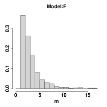
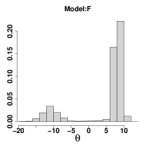
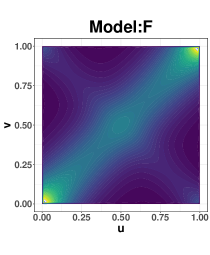
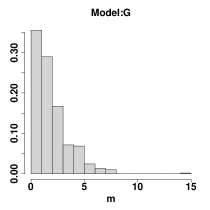
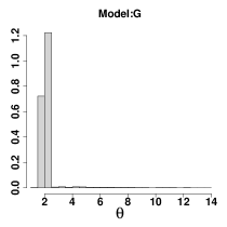
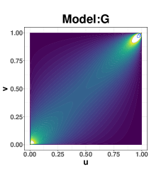
Figure 6: Occupancy data for day 5. Posterior fittings for top two best models. Frank (top row) and Gumbel (bottom row). Across columns: Number of components (1st), $\theta_{i}$’s (2nd), and bivariate density (3rd).

To assess model fit we computed the LPML gof statistic and obtained the following values: 72.64 for the AMH, 88.97 for the Clayton, 102.59 for the Frank, 92.48 for the Joe, and 105.15 for the Gumbel. Clearly the two best models are the Frank and the Gumbel. In Figure 6 we report posterior inferences for these two models. The number of components obtained with the Frank model has a mode at 2 and the histogram of the posterior values of the parameters $\theta_{i}$ is bimodal with a heavier mode in a positive value around $8$ and a lighter mode in a negative value around $-11$. The density estimate shows the cross shape of the original data. On the other hand, with the Gumbel model the number of components has mode at 1 with the copula parameters $\theta_{i}$ concentrated around 2. The density estimate shows the positive dependence with wide contours in the center resembling the negative dependence.

Empirical Kendall’s tau for he data is $0.462$ and the corresponding estimates with the Frank mixture model is $0.41$ with a 95% CI of $(0.28,0.84)$; and for the Gumbel model we get $0.51$ with a 95% CI of $(0.46,0.74)$. Although both CI from both models contain the empirical value and they intersect in a large amount of values, the Gumbel model is estimating a slightly larger association.

Using our procedure to estimate the number of components, in Table 7 we report two clusters for the Frank copula with estimated copula parameters at $8.46$ with a weight of $82.5\%$ for the first component and at $-12.8$ with a weight of $17.5\%$ for the second component. For the Gumbel copula, a single cluster is determined with parameter value estimated between $1.87$ and $2.26$ with $95\%$ probability. An advantage of the Gumbel model is that it has right-upper tail dependence and the data seem to support this.

Again, we also compare with the competing model BSA. The LPML statistic obtained is 78.40, which is better that the fit with the AMH kernel but worst than the fitting obtained with the other four kernels.

4.3 Multivariate simulation study

We now consider a vector of dimension four, i.e., ${\bf U}=(U_{1},U_{2},U_{3},U_{4})$ coming from a mixture of three Clayton copulas $f({\bf u})=\sum_{j=1}^{3}\pi_{j}f_{C}({\bf u}\mid\vartheta_{j})$, with $\boldsymbol{\pi}=(0.2,0.3,0.5)$ and three different sets of copula parameters that we denote as setting 1: $\boldsymbol{\vartheta}=(1,5,15)$; setting 2: $\boldsymbol{\vartheta}=(2,5,10)$; and setting 3: $\boldsymbol{\vartheta}=(2,7,15)$. We sampled $n=500$ data points from each of these three settings.

We fitted our Bayesian nonparametric mixture model with Clayton kernel. Hyper parameters are: $c_{\theta}=d_{\theta}=0.01$, $p_{a}=1$, $q_{a}=5$, $c_{b}=1$ and $d_{b}=10$. The MCMC was run for 10,000 iterations with a burn-in of 5,000.

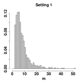
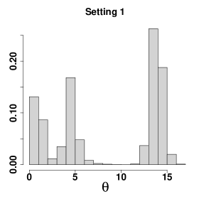
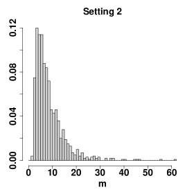
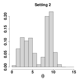
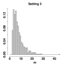
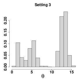
Figure 7: Simulated four-dimensions data from a mixture of 3 Clayton components with weights $\boldsymbol{\pi}=(0.2,0.3,0.5)$ and different copula paramters: $\boldsymbol{\vartheta}=(1,5,15)$ (top), $\boldsymbol{\vartheta}=(2,5,10)$ (middle) and $\boldsymbol{\vartheta}=(2,7,15)$ (bottom).Posterior distribution of the number of components (left) and model parameters (right).

Posterior distribution for the number of components and for copula parameters are included in Figure 7. The number of components has a mode at 6, 4 and 4 for the three settings, respectively, but the posterior distribution on the copula parameters is three-modal in the three settings, with modes around the true values.

True and estimated Kendall’s tau are reported in Table 8. Point estimates (posterior mean) are very close to the true values and 95% CI all contain the true association parameters.

In order to report a single clustering, we performed our five values search around the mode, presented in Section 3.3. Results are shown in Table 9. For setting 1, our procedure selects 8 groups, but the first three groups account for 84% of the total weight. We note the shrinkage towards the center values. The first group has a weight of 0.56, similar to the theoretical 0.5 with 95% CI $(12.8,14.5)$, slightly inferior to the true value of $15$. However, the other two theoretical components seem to be split into three or four components.

For setting 2, our procedure selects 4 groups, with the first one clearly associated to the third true mixture component with a weight of $0.58$ and a parameter CI of $(8.7,9.8)$ slightly smaller than $10$, the second group with a weight of $0.16$ and a parameter CI of $(1.6,2.25)$, and the third and fourth groups seems to be associated to the second true mixture component. Finally for setting 3, our procedure selects 6 groups with the first group being the one with highest weight, associated to the third true mixture component, and the last five groups associated to the first two mixture components.

4.4 Multivariate real data analysis

With the objective to measure the inequality in Mexico, the Population National Council (CONAPO) created in the year 1990 a poverty (marginality) index for each of the more than 2,400 municipalities in Mexico. Since then, every five years CONAPO updates the index using the most recent household surveys, including the census.

The poverty index is formed by four dimensions measured in nine variables. Education dimension: percentage of illiterate people older than 15 years old (ANALF), percentage of people older than 15 years old without complete basic education (SBASC); household dimension: percentage of household occupants without sewage and toilet (OVSDE), percentage of household occupants without electricity (OVSEE), percentage of household occupants without tap water (OVSAE), percentage of household occupants with dirt floor (OVPT), percentage of household occupants in overcrowding (VHAC); Population distribution dimension: percentage of people that lives in towns with less that 5,000 inhabitants (PL5000); income dimension: percentage of employed people with an income of less than two minimum wages (PO2SM).

We concentrate on the poverty variables of the house dimension OVSDE ($X_{1}$), OVSEE ($X_{2}$) and OVSAE ($X_{3}$) for the state of Puebla in Mexico. This state has 217 municipalities in urban and rural areas. Data is available at https://www.gob.mx/conapo/documentos/indices-de-marginacion-2020-284372.

A simple exploratory graphical analysis (see Figure 8) shows that these three variables show a positive dependence with empirical kendall’s taus of $\tau_{1,2}=0.326$, $\tau_{1,3}=0.343$ and $\tau_{2,3}=0.318$, which suggests that a mixture of Archimedean copulas is a good model for these data.

We fitted our Bayesian nonparametric mixture model with different kernels. Hyperparameters are the same as in the multivariate simulation study. The MCMC was run for 10,000 iterations with a burn-in of 5,000. The LPML gof measures are 72.93 for the Clayton, 55.55 for the Frank, and 44.47 for the Gumbel.

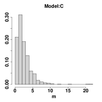
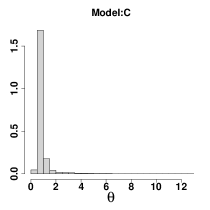
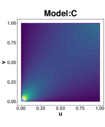
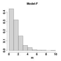
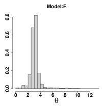
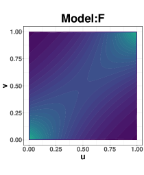
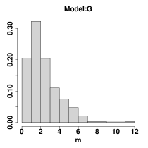
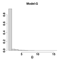
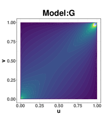
Figure 9: Multivariate real data. Posterior distributions for the number of components, copula parameters, and bivariate density estimates.

Posterior distributions for the number of components $m$, model parameters $\theta$ and bivariate density heatmaps are shown in Figure 9. Posterior mode for the number of components is two for the Clayton, one for the Frank, and two for the Gumbel. Model parameters are around one for the Clayton, between 2 and 4 for the Frank and around one for the Gumbel. Bivariate densities are very similar with the three models, but with a strong lower-left tail dependence characteristic of the Clayton and an upper-right tail dependence in the Gumbel. By looking at the dispersion diagrams of the data, the lower-left tail dependence of the Clayton seems to be more appropriate and also supported by the LPML values.

Posterior estimation of the Kendall’s tau, for the best fitting model, Clayton, is $0.302$ as point estimate with a 95% CI of $(0.22,0.53)$. Clearly the CI contains the three empirical Kendall’s tau pairwise association parameters among the three poverty variables. Implementing our clustering selection procedure we obtain one group with copula parameter estimated at $0.84$ with a 95% CI $(0.69,0.99)$.

5 Concluding remarks

We propose Bayesian inference for a nonparametric mixture model of Archimedean copulas. Our model depends on the multivariate Archimedean copula densities, which require as many derivatives as the dimension of the data. Depending on the specific Archimedean family, some of the required derivatives are more difficult to compute than others. For instance, derivatives for the Clayton, Gumbel, and Frank families are comparatively straightforward to obtain using the R codes that are available at copula R-package by Hofert et al., (2023) .

The runtime to fit our model significantly depends on the number of clusters chosen in each iteration. This in turn depends on the data size and the specific data. For 2 to 4 clusters and with approximately 200 observations, in a 3-dimensional space, and over 10,000 iterations, the computation completes within an hour.

Due to the construction of the Archimedean copulas, pairwise Kendall’s tau coefficients for the elements in a vector are the same. For allowing different Kendall’s tau coefficients in different pair of variables, an extension like hierarchical Archimedean copulas could be used (Li et al., (2021); Hofert & Pham, (2013)). We leave this as future work.

Copula	$\phi_{\theta}(t)$	$\Theta$	$\tau_{\theta}$
AMH	$\log\left\{\frac{1-\theta(1-t)}{t}\right\}$	$[-1,1]$	$1-2\{\theta+(1-\theta^{2})\log(1-\theta)\}/(3\theta^{2})$
CLA	$t^{-\theta}-1$	$[-1,\infty)$	$\theta/(\theta+2)$
FRA	$-\log\left\{\frac{\exp(-\theta t)-1}{\exp(-\theta)-1}\right\}$	$\mathbb{R}$	$1-4\{1-D_{1}(\theta)\}/\theta$
GUM	$(-\log t)^{\theta}$	$[1,\infty)$	$1-1/\theta$
JOE	$-\log\left\{1-(1-t)^{\theta}\right\}$	$[0.238734,\infty)$	$1-4\sum_{k=1}^{\infty}1/\{k(\theta k+2)\{\theta(k-1)+2\}\}$

Table 1: Five most common Archimedean families and properties. The Debye function of order one is given by $D_{1}(\theta)=(1/\theta)\int_{0}^{\theta}t/(e^{t}-1)\mbox{d}t$.

Copula	$\phi_{\theta}^{(1)}(t)$	$\phi_{\theta}^{(2)}(t)$
AMH	$\frac{\theta-1}{t\{1-\theta(1-t)\}}$	$\frac{(1-\theta)(1-\theta+2\theta t)}{\left\{t(1-\theta(1-t))\right\}^{2}}$
CLA	$-\theta t^{-(\theta+1)}$	$\theta(\theta+1)t^{-(\theta+2)}$
FRA	$\frac{\theta\exp(-\theta t)}{\exp(-\theta t)-1}$	$\frac{\theta^{2}\exp(-\theta t)}{\{\exp(-\theta t)-1\}^{2}}$
GUM	$-\frac{\theta}{t}(-\log t)^{\theta-1}$	$\frac{\theta}{t^{2}}(-\log t)^{\theta-1}+\frac{\theta(\theta-1)}{t^{2}}(-\log t)^{\theta-2}$
JOE	$\frac{-\theta(1-t)^{\theta-1}}{1-(1-t)^{\theta}}$	$\frac{\theta(\theta-1)(1-t)^{\theta-2}+\theta(1-t)^{2\theta-2}}{\{1-(1-t)^{\theta}\}^{2}}$

Table 2: First and second derivatives of the five most common Archimedean families.

Data / Model	AMH	CLA	FRA	JOE	GUM	BSA
AMH	0.52	0.41	0.03	3.21	-0.14	-4.32
CLA	12.61	161.23	75.24	51.74	76.18	7.40
FRA	-0.12	5.65	7.33	4.45	4.13	-3.01
JOE	37.49	76.78	101.80	125.80	112.80	55.33
GUM	77.84	198.79	238.16	270.01	276.52	100.14

Table 3: Bivariate simulated data. LPML statistics when taking a sample of size $n=200$ and fitting the five models. Competing model in the last column.

Data / Model	AMH	CLA	FRA	JOE	GUM	BSA
AMH	0.92	0.45	-0.63	3.29	-1.52	-4.01
CLA	28.55	362.57	203.09	147.09	171.77	1.83
FRA	2.26	8.90	22.91	22.21	0.87	6.59
JOE	95.62	209.85	229.84	298.60	291.43	97.60
GUM	226.25	596.56	648.30	678.80	718.82	172.86

Table 4: Bivariate simulated data. LPML statistics when taking a sample of size $n=500$ and fitting the five models. Competing model in the last column.

	True	Emp	AMH	FRA	CLA	JOE	GUM
AMH	0.04	0.01	0.02	0.02	0.04	-0.04	0.05
CLA	0.25	0.14	0.11	0.22	0.25	0.22	0.34
FRA	0	-0.07	-0.04	-0.06	0.00	-0.09	0.06
JOE	0.59	0.54	0.30	0.58	0.47	0.61	0.61
GUM	0.85	0.84	0.33	0.83	0.78	0.81	0.84

Table 5: Bivariate simulated data. True, empirical and estimated Kendall’s tau with $n=500$.

	$\theta_{1}$	$\theta_{2}$	$\theta_{3}$	$\theta_{4}$
Model: AMH (-0.8, 0.8)
mean	0.078
$q_{2.5}$	-0.208
$q_{97.5}$	0.311
weight	0.999
Model: CLA (-0.5, 10)
mean	-0.502	11.650
$q_{2.5}$	-0.504	10.276
$q_{97.5}$	-0.497	12.961
weight	0.506	0.494
Model: FRA (-5, 5)
mean	-6.468	5.449	3.759	-1.276
$q_{2.5}$	-7.340	4.393	2.270	-6.120
$q_{97.5}$	-5.534	6.548	5.494	4.172
weight	0.545	0.316	0.128	0.010
Model: JOE (2, 10)
mean	11.213	1.995	5.823
$q_{2.5}$	10.022	1.759	4.245
$q_{97.5}$	12.519	2.233	7.927
weight	0.474	0.466	0.060
Model: GUM (5, 10)
mean	10.063	3.258	5.954
$q_{2.5}$	9.282	2.781	2.568
$q_{97.5}$	10.930	3.738	11.336
weight	0.749	0.248	0.002

Table 6: Bivariate simulated data. Post MCMC summaries given chosen c.c.

	$\theta_{1}$	$\theta_{2}$	$\theta_{1}$
Model	FRA		GUM
mean	8.463	-12.755	2.048
$q_{2.5}$	7.389	-15.997	1.873
$q_{97.5}$	9.773	-9.614	2.259
weight	0.824	0.175	0.999

Table 7: Occupancy data. Post MCMC summaries given chosen c.c.

Setting	$\tau$	$\widehat{\tau}$	95% CI
1	0.722	0.702	(0.288, 0.883)
2	0.731	0.716	(0.413, 0.841)
3	0.775	0.758	(0.409, 0.879)

Table 8: Multivariate simulated data. True and estimated Kendall’s tau.

	$\theta_{1}$	$\theta_{2}$	$\theta_{3}$	$\theta_{4}$	$\theta_{5}$	$\theta_{6}$	$\theta_{7}$	$\theta_{8}$
Setting 1: $\boldsymbol{\pi}=(0.2,0.3,0.5),\boldsymbol{\theta}=(1,5,15)$
mean	13.703	1.181	4.409	1.801	4.350	0.632	1.754	1.763
$q_{2.5}$	12.834	0.964	3.773	1.298	3.366	0.179	0.677	0.215
$q_{97.5}$	14.535	1.430	5.045	2.336	5.448	1.135	2.941	4.122
weight	0.559	0.168	0.108	0.070	0.056	0.030	0.006	0.002
Setting 2: $\boldsymbol{\pi}=(0.2,0.3,0.5),\boldsymbol{\theta}=(2,5,10)$
mean	9.215	1.907	4.184	3.000
$q_{2.5}$	8.673	1.593	3.641	2.504
$q_{97.5}$	9.784	2.246	4.747	3.502
weight	0.575	0.158	0.146	0.120
Setting 3: $\boldsymbol{\pi}=(0.2,0.3,0.5),\boldsymbol{\theta}=(2,7,15)$
mean	12.205	4.138	1.494	3.129	3.294	1.149
$q_{2.5}$	11.591	3.591	1.132	2.344	2.045	0.394
$q_{97.5}$	12.889	4.702	1.865	3.970	4.830	1.950
weight	0.677	0.160	0.090	0.048	0.014	0.010

Table 9: Multivariate simulated data. Post MCMC summaries given chosen c.c.

Figure 1: Kendall’s tau for the five Archimedean families of Table 1 as a function of $\theta$.

Figure 5: Occupancy data for day 5. Humidity ratio (HR) versus carbon dioxide (CO2).

Figure 8: Multivariate real data. Pairwise scatterplot of the three variables.