Multiple Orthogonal Polynomials of two real variables
Lidia Fernández and Juan Antonio Villegas
Lidia Fernández
IMAG and Departamento de Matemática Aplicada
Universidad de Granada
18071, Granada, Spain.
lidiafr@ugr.esJuan Antonio Villegas
IMAG and Departamento de Matemática Aplicada
Universidad de Granada
18071, Granada, Spain
jantoniovr@ugr.es
Abstract.
Polynomials known as Multiple Orthogonal Polynomials in a single variable are polynomials that satisfy orthogonality conditions concerning multiple measures and play a significant role in several applications such as Hermite-Padé approximation, random matrix theory or integrable systems. However, this theory has only been studied in the univariate case. We give a generalization of Multiple Orthogonal Polynomials for two variables. Moreover, an extended version of some of the main properties are given. Additionally, some examples are given along the paper.
Key words and phrases:
Multiple Orthogonal Polynomials, Bivariate Orthogonal Polynomial Vectors, Graded Reverse Lexicographic Order, Type I Multiple Orthogonal Polynomials, Type II Multiple Orthogonal Polynomials, Biorthogonality Relation, Nearest Neighbours Recurrence Relations
2010 Mathematics Subject Classification:
33C45, 42C05
The work of the authors was partially supported by IMAG-María de Maeztu grant CEX2020-001105-M.
1. Introduction
Multiple Orthogonality is a theory that extends standard orthogonality. In this framework, polynomials (defined on the real line in this introduction) satisfy orthogonality relations with respect to more than one measure. There are some results for Multiple Orthogonal Polynomials (MOP) that generalize their standard antecedents. For instance, the well-known theorem of existence and unicity of orthogonal polynomials sequences for a fixed real measure concerning its moments Hankel matrix has a generalization for Multiple Orthogonal Polynomials. Additionally, more extended results such as “Nearest Neighbour Relations” [26], which generalize the three-term recurrence relation, will be shown in Section 2.
Moreover, this extension has been widely studied recently, due to its applications in other mathematics branches [23]. An introduction to multiple orthogonality and its properties can be found in [1], [17] or [27]. Some examples of applications of this theory are Hermite-Padé rational approximation [25], Bessel functions and Bessel paths [8, 20], electrostatics [22] or Markov chains and random walks [5, 7, 6].
As shown, several researchers study and focus on this topic. However, Multiple Orthogonal Polynomials have been studied only in the univariate case. In this moment, there is no extension of the definitions and main results of multiple orthogonality employing bivariate polynomials, nor of its applications.
Nevertheless, it is possible to manage with standard orthogonal polynomials in the multivariate case. There are two different approaches. In 1975, T. Koornwinder employed the graded reverse lexicographic order in the usual basis of the space of multivariate polynomials to extend the standard definitions [18]. This order has been employed to extend some families of multivariate orthogonal polynomials [4], and a similar order was applied to the Laurent monomials to study bivariate orthogonal Laurent polynomials [9]. On the other hand, it is possible to bring polynomials of equal degree together and use polynomial vectors [14]. This approach has been employed to study a bi-dimensional version of Toda equations [3], or Quasi-birth-and-death processes [16, 15], among others. More of these generalizations will be discused in Section 3. Some applications of orthogonal polynomials like Gaussian cubature or Padé approximation has also been generalized to the bivariate case [2, 10, 11, 12, 13].
The structure of this article is the following. Firstly, in Section 2, we fix the notations and present the main definitions of multiple orthogonality in one variable: Type I and Type II MOP, together with a result which characterizes the existence of these polynomials. Next, in Section 3, two definitions of Type I and II bivariate MOP are shown. Additionally, these definitions are presented by using polynomial vectors. Following, some main results of the univariate case generalized to the bivariate one are presented in Section 4: Existence and unicity of bivariate MOP, Biorthogonality relation and Nearest Neighbour Recurrence Relations. Previous to the conclusions, in Section 5, we find a relationship between the univariate and the bivariate cases, discussing the product of two univariate Type II MOP as a bivariate MOP.
2. Preliminaries: Multiple Orthogonal Polynomials of one real variable
First, let us consider different real measures such that , . We will use multi-indices , and denote , the so called modulus or norm of . These multi-indices will determine the orthogonality relations with each measure and the degree of the polynomials.
For a fixed measure , , we denote its associated integral inner product as
(1)
There are two different types of multiple orthogonality, which will be explained shortly. More information and a deeper introduction to multiple orthogonality can be found in [17, Section 23.1] or [27, Section 1].
Definition 2.1(Type II Multiple Orthogonal Polynomials).
Let . A monic polynomial is a Type II Multiple Orthogonal Polynomial if and
(2)
This means is orthogonal to with respect to each measure , .
On the other hand, there exists another type of multiple orthogonality: Type I multiple orthogonality.
Definition 2.2(Type I Multiple Orthogonal Polynomials).
Let . Type I Multiple Orthogonal Polynomials are polynomials , where , and satisfying
(3)
Whenever the measures are all absolutely continuous with respect to a common positive measure defined in , i.e., , , it is possible to define the Type I function as
(4)
Using the Type I function, the orthogonality relations (3) could be written as
(5)
Nevertheless, neither all systems of measures nor all multi-indices yield a Type I vector of polynomials or a Type II polynomial, just as in standard OP theory, where not every measure produces an OPS , depending on the Hankel matrix of moments. In this sense, there is an analogous result for existence and unicity of MOP.
Proposition 2.3.
[17, Section 23.1]
Given a multi-index and positive measures, , the following statements are equivalent:
(1)
There exist a unique vector of Type I MOP.
(2)
There exist a unique Type II MOP .
(3)
The following block matrix of moments is regular:
(6)
and are the moments of the measures, .
This means that, for a fixed multi-index, Type I MOP associated to this multi-index exists if and only if Type II MOP exists. Following Proposition 2.3, we provide the next definition.
Definition 2.4.
A multi-index is normal if it satisfies the conditions in Proposition 2.3.
A system of measures is perfect if every is normal.
Some examples of perfect systems are Angelesco systems, AT-systems and Nikishin systems, see [17, Sections 23.1.1 and 23.1.2], [24].
3. Multiple Orthogonal polynomials of two real variables
In the bivariate case, it is possible to deal with Orthogonal Polynomials by using two different approaches. In [14], C. Dunkl and Y. Xu employ a polynomial vector notation, so that, if we denote as the vector of all monomials of total degree , whose size is , we can express a polynomial vector of degree as
where is a matrix and is regular. With this notation, it is possible to extend the standard orthogonality definitions and results to polynomial vectors, see [14, Chapter 3].
A different approach can be found in [18], where T. Koornwinder uses the basis of the vector space of bivariate polynomials ordered by the graded reverse lexicographic order, this is
(7)
Our extension to the bivariate case of multiple orthogonality is mainly focused in this second approach, although some properties will be also presented by using polynomial vectors in order to clarify some notations.
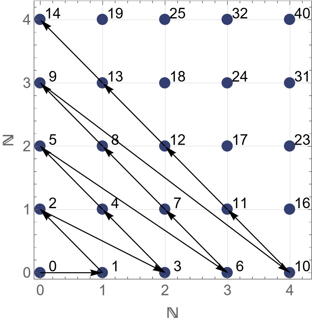
Previous to our definitions, remember that the Cantor Pairing Function, , is a bijection between and (see [21]). Its expression is given by
(8)
In Figure 1 you can observe a graphic representation of this bijection.
Figure 1. Graphic representation of Cantor Pairing Function
Using the Cantor Pairing Function, it is possible to assign a natural number to each monomial of the basis (7), so that is associated to , to , to , and so on. Following this idea, given a bivariate polynomial , you can express as a linear combination of the first elements of (7), in a way that
We will refer as the multidegree of , denoted by , to the pair , which are the exponents of the variables ‘’ and ‘’ (in that order) of the leading term. Applying the function to that pair, observe is the position of the leading monomial in the list (7), starting the count at . Next, we present some useful definitions associated to every multi-index.
Definition 3.1(Degree and Remainder).
For every multi-index , let us consider , the modulus of , and let be the pair such that . We define the degree and the remainder associated to as
(9)
This means that it is possible to write
Remark 3.2.
For every and every multi-index such that
Example 3.3.
In Table 1 some examples of multi-indices for some values of and their associated values of the modulus, multidegree, degree and remainder are shown.
Table 1. Parameters associated to multi-indices
Remember that, in the univariate case, was the number of orthogonality conditions of both Type I and II MOP, and it was also the degree of the Type II MOP. In our generalization, given below, is also the number of orthogonality conditions, but, instead of the degree of the bivariate Type II MOP, in this case it is the position of its leading term in (7), i.e., . As a consequence, is the actual degree of .
Now, given , and a system of -dimensional measures , we present the definitions of Type I and II multiple orthogonality.
Definition 3.4(Type II Bivariate Multiple Orthogonality).
Let and such that . Take a multi-index such that . Then, the monic polynomial
is the bivariate Type II Multiple Orthogonal Polynomial associated to if it satisfies the orthogonality conditions
(10)
Observe that, as mencioned, and , where is the degree associated to (see Definition 3.1).
Definition 3.5(Type I Bivariate Multiple Orthogonality).
Let be a multi-index. For each , consider such that , . Then, the polynomials given by
are the bivariate Type I Multiple Orthogonal Polynomials if they satisfy the orthogonality conditions
(11)
In this case, we have , .
Once again, let us assume the measures are absolutely continuous with respect to a common measure whose support is , where (this is, ). Then, we define the Bivariate Type I Function as
In order to clarify this definitions, we will introduce the following example.
Example 3.6.
Consider a system of bidimensional measures. If we choose and , we have to choose a multi-index such that , for example . As , then and .
Assuming the existence, which will be discussed later, the bivariate Type II MOP will have the following shape:
and it will satisfy
Note that, indeed, .
On the other hand, the bivariate Type I MOPs will have the following shape:
and they will satisfy
In order to bring polynomials of equal degree together and clarify some notations according to [14], we extended Definitions 3.4 and 3.5 to polynomial vectors, which we will call bivariate Multiple Orthogonal Polynomial Vectors (MOPV). But first, let us establish some conditions regarding the multi-indices and parameters that will be employed. Given , we know there are different monomials of degree . Following the order established by the application , the first multidegree is (associated to the monomial ). From this point, choose multi-indices such that
•
The modulus of the multi-indices satisfy
This is,
(14)
As a result, every multi-index is associated to a bivariate Type II MOP of degree .
•
They are neighbour multi-indices, i.e.
(15)
where , for certain .
Under these conditions, it is possible to construct a degree polynomial vector, employing multi-indices satisfying conditions (14) and (15). We will denote as the components of the multi-index , .
Definition 3.7(Bivariate Type II Multiple Orthogonal Polynomial Vector).
Given , consider multi-indices satisfying conditions (14) and (15). For each multi-index , let be its associated bivariate Type II MOP of Definition 3.4. The polynomial vector
where is a matrix and is a lower triangular matrix with ones on the diagonal, is the Bivariate Type II Multiple Orthogonal Polynomial Vector associated to and it satisfies
where the -th row has its first components equal to , , .
Remark 3.8.
The polynomial vector is composed of polynomials of degree so that their leading terms are .
In order to clarify this definition, we present an example.
Example 3.9.
Let us take , , then, we need to choose three neighbour multi-indices so that . Consider, for example, . Then
satisfying
since the first components of each pair are 1, 1 and 2.
since the second components of each pair are 2, 3 and 3.
Following this idea, we could also define the bivariate Type I MOPVs. In this case, we define polynomial vectors of different degree but necessarily same size.
Definition 3.10(Type I Multiple Orthogonal Polynomial Vectors).
Given , consider multi-indices satisfying conditions (14) and (15). For each multi-index , let be its associated bivariate Type I MOP of Definition 3.5. The polynomial vectors
are the Bivariate Type I Multiple Orthogonal Polynomial Vectors associated to , and they satisfy
where the -th row has its first components equal to and the -th component is , , .
Remark 3.11.
As mentioned, the polynomial is the -th Type I MOP of Definition 3.5 for the multi-index . Then, . Besides, observe that all polynomial vectors have the same size () and there are as many bivariate Type I MOPV as measures, .
Naturally, the Bivariate Type I Vector is defined as
(16)
Observe the following example, where we use the same parameters and the same multi-indices as in Example 3.9.
Example 3.12.
Let us take , , then , and we consider . Then, the bivariate Type I MOPV are
and they satisfy
since .
In the next sections, we will present generalized versions of some results from the univariate case employing Definitions 3.4 and 3.5, and some analogous when the vector notation of Definitions 3.7 and 3.10 is applied.
4. Main Results
We will start with the existence of bivariate Type I and/or Type II MOP. Given a multi-index , we will denote by the following block matrix:
(17)
where, for every :
(18)
where are the moments of the bidimensional measures. Observe that the value in the -th row and the -th column of (starting the count in 0) is , , .
For bivariate Type II MOP, applying conditions (10) to a generic monic polynomial, it is easy to deduce that the coefficients of this polynomial are the solutions of the linear system
with
Besides, applying (11) to generic bivariate Type I MOPs, we obtain that the coefficients of bivariate Type I MOPs are the solutions of the system
Then, for a fixed multi-index , Type I and Type II will exist if and only if the matrix is regular. So, we have the following result, which clearly generalizes Proposition 2.3.
Proposition 4.1.
Given a system of bidimensional measures and a multi-index , the following statements are equivalent.
As happened in the univariate case, we have a matrix whose regularity for a fixed multi-index ensures the existence and unicity of both Type I and II bivariate MOP. Additionally, for a fixed multi-index, bivariate Type I MOPs exist if, and only if, bivariate Type II MOP exists. This proposition motivates the following definitions.
Definition 4.2.
Given a system of bidimensional measures and a multi-index , is said to be normal if it satisfies the conditions in Proposition 4.1, and the system of measures is a perfect system of measures if every multi-index is normal.
See the following example to clarify the structure of these matrices.
Example 4.3.
Let us consider a system of bidimensional measures and a multi-index . Then, bivariate Type I and Type II MOPs associated to in the system of measures exist if and only if the matrix
is regular. In that case, would be a normal multi-index.
Observe that, regarding the shape of the matrix , defined in (17) and (18), is composed of blocks: the first one of size , whereas the remaining blocks size is .
If we use the polynomial vector notation, it is clear that, for a set of multi-indices satisfying conditions (14) and (15), the existence of bivariate Type II MOPV is equivalent to the existence of bivariate Type I MOPVs and both are equivalent to the regularity of all matrices .
Another basic result in multiple orthogonality, which is a consequence of the definition itself, is a biorthogonality relation satisfied by Type II and Type I MOP (see [17, Theorem 23.1.6]). We have proven a generalization of this theorem.
Theorem 4.4.
Let be a system of bivariate absolutely continuous measures and consider two normal multi-indices . Then, the bivariate Type II MOP and the bivariate Type I function satisfy the following biorthogonality relation:
(19)
Proof.
Applying the definition of Type I function in (12),
•
If (componentwise), then for every . As we know from Definition 3.4, , due to Type II orthogonality for every .
•
If , then , so that because of Type I orthogonality.
•
If , then and, again due to Type I orthogonality and because is a monic polynomial, .
∎
If we want to express this orthogonality relation with bivariate MOPV, recall that the result of applying an inner product to two vectors of functions is a matrix whose entries are the scalar inner product applied componentwise:
So, the relation is:
Corollary 4.5.
Consider and , two sets of and normal multi-indices satisfying conditions (14) and (15). Then, the bivariate Type II MOPV defined in Definition 3.7 and the bivariate Type I Function defined in (16) satisfy the following relation:
Equation (20) may appear quite asymmetric. This is a consequence of the asymmetry of equation (19), where the result is if . Even the original univariate biorthogonality relation in [17] shares this lack of symmetry.
The next relations we are going to generalize are the ‘Nearest Neighbours Recurrence Relations’, which are in turn generalizations of the three-term relation by using MOPs (see [17, Theorem 23.1.7, Theorem 23.1.9]).
Since we are working with multi-indices and bivariate polynomials, there are several ways to decrease or increase the degree or the multidegree of a bivariate MOP. For example, given two multi-indices such that componentwise, we know that
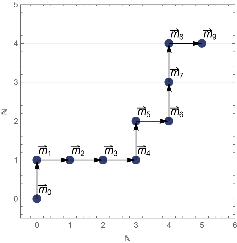
and as a consequence, . Along the remainder of this section, we will consider paths from to via , with , , and where in each step the multi-index is increased by one at exactly one component, i.e., the path is composed of neighbour multi-indices (they satisfy condition (15) ). For these paths, we have and . See Figure 2 for an example of these kind of path.
Figure 2. A path from to for
Whereas the bivariate biorthogonality relation is almost the same as the univariate one in [17, Theorem 23.1.6], we will show that the extended Nearest Neighbour Relations (NNR) are different; however, this issue can be solved by using the vector notation. There are two different types of NNR, one employs bivariate Type II MOP while the other one uses bivariate Type I MOP (Type I functions, actually).
Firstly, we will focus on the NNR for bivariate Type II MOP. Given , the original univariate Nearest Neighbours Relation [17, Theorem 23.1.7] expresses the polynomial as a linear combination of itself, a neighbour of higher degree and neighbours of lower degree. In this case, it is clear that , and that is the reason why only one neighbour of higher degree is needed. However, this equality does not hold in the bivariate case, since , and something similar happens when we multiply by ‘’. For this reason, we present the following lemma.
Lemma 4.6.
Let
so that . Then,
where is the total degree of .
Proof.
Remember the usual basis of the vector space of bivariate polynomials ordered by the reverse lexicographic graded order (7):
An alternative interpretation of the function is the position of the monomial on this list (starting the count in ). In this way, there are monomials in between and . Thus, . For the second equality, observe the monomial is exactly the next one after .
∎
With this, we can present different results of NNR for Type II bivariate MOP.
Theorem 4.7(Nearest Neighbour Relation (for and )).
Let us consider , a perfect system of bidimensional measures, a multi-index , its associated bivariate Type II MOP and its degree and remainder introduced in Definition 3.1. Define . Choose such that
and componentwise, and let be their associated bivariate Type II MOP. Consider a path of neighbour multi-indices where for every , , , and . For every , let be the bivariate Type II MOP and the bivariate Type I function (12) associated to the multi-index . Then, the following relations hold:
(21)
(22)
where and .
Proof.
We will prove (21). The proof of (22) is analogous but using the second equation of Lemma 4.6 instead of the first one when necessary.
Let us consider a path of neighbour multi-indices where , , , and .
According to Lemma 4.6, we know that . In addition, as is monic, so is . On the other hand, as , then is a basis of the vector space of bivariate polynomials such that . With all this information, it is possible to write as a linear combination of .
(23)
In order to find the values of coefficients , for , observe
(24)
To simplify the previous expression, we will employ the biorthogonality relation of Theorem 4.4.
•
Firstly, it is known that if, and only if , then if .
The next step is to prove that , i.e., for . Applying (12):
and because of the integral definition of these inner products
Fixing , and due to Type II orthogonality, we know that
Now, remember and, in this case, , so that necessarily, and . With these inequalities and using Lemma 4.6 we have
Then, for and for .
∎
Due to the little difference in the behaviour of the variables ‘’ and ‘’ shown in Lemma 4.6, we also have some differences in the items of this last theorem. On one hand, in (22) there are multi-indices of higher norm, one more than in (21). On the other hand, in both items we employ multi-indices of lower norm. To clarify this result, we present an example.
Example 4.8.
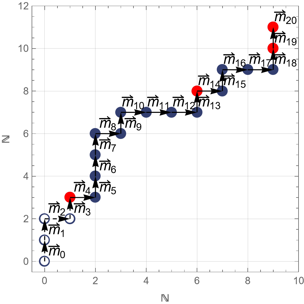
Assume , , then , , , , and we need s.t. and , let us take, for example and . Now, we choose a path from to via , and .
Then
(26)
Observe Figure 3(a), where we represent the multi-indices employed in the linear combinations (26). As shown, multi-indices whose norms are higher than and multi-indices whose norms are lower than are used. and do not take place in (26).
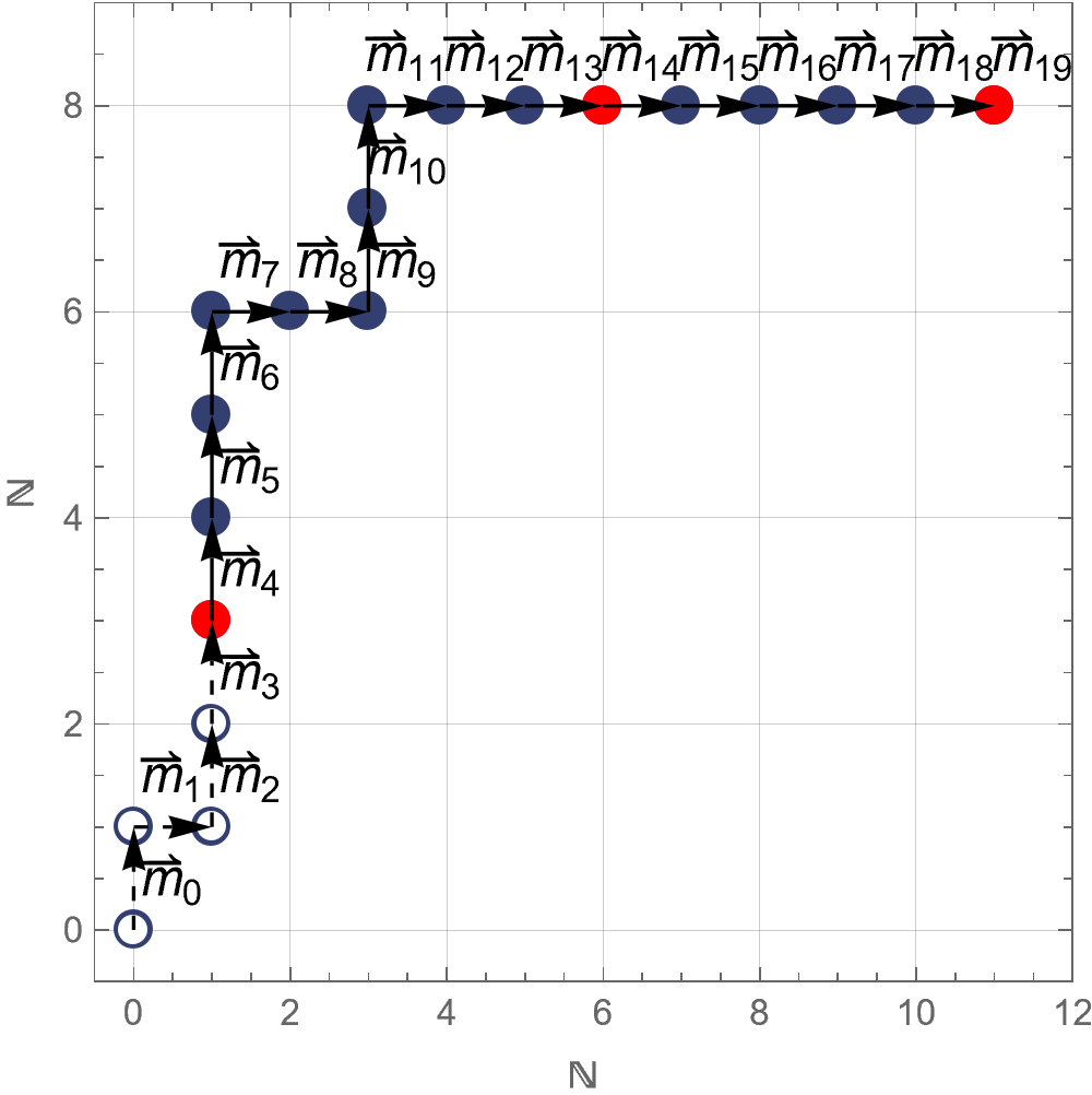
Additionally, the relation still holds if we choose a different path from to , and even if we choose another or . For example, considering the following path (see Figure 3(b)):
Then
(27)
(a)
(b)
Figure 3. Example of NNR for bivariate Type II MOP
When using the NNR, the polynomial vector notation is really useful for clarifying the relation and its notation. Remember a proper bivariate Type II MOPV is composed of polynomials whose leading terms are, respectively, , so that . So, if we bring all the polynomials of equal degree together in polynomial vectors, it is possible to obtain a vector version of the NNR.
Corollary 4.9(Nearest Neighbour Relation (for and )).
Let be a perfect system of bidimensional measures. Consider and multi-indices satisfying (14) and (15) and their associated bivariate Type II MOPV . Define
and let be a path of neighbour multi-indices with , where the last multi-index is a neighbour of and the multi-index belongs to the path. This means, there exists with
Let be the bivariate Type II MOPV associated to the set of multi-indices , . Choose satisfying (14) and (15), and is a neighbour of . Let be the bivariate Type II MOPV associated.
Then
and
where and are matrices of dimension , and .
Proof.
In this proof, only the relation for will be proven. The arguments for are analogous but applying the second equation of Lemma 4.6.
Similarly to the proof of Theorem 4.7, let us consider a path of neighbour multi-indices
so that , and .
For , we know the polynomial vectors are composed of polynomials of degree and their leading terms are . Furthermore, the polynomial vector (resp. ) is composed of (resp. ) polynomials of degree (resp. ) and their leading terms are (resp. ). Then, the polynomial vectors
shape a basis of the space of polynomial vectors of degree (where the coefficients of the linear combinations are matrices of proper dimension). It is clear that is a polynomial vector composed of polynomials of degree . Then, it is possible to express
(28)
where are matrices of dimension for .
Observe that the leading terms of (resp. ) are the same as the leading terms of the first (resp. last) polynomials of . Then, necessarily (resp. ).
Now, we want to show that . First, if we multiply (28) by the Type I Function we get
(29)
Applying the biorthogonality relation for bivariate MOPV (20), we get that, for a fixed :
Then, observe the first summand is a matrix whose first column is and the other columns are the first columns of . On the other hand, the second summand is a matrix where the first column is the last column of and the remaining columns are . So, we have that is equal to a matrix whose first column is the last column of and the other columns are the first columns of . This means:
(30)
So, we have to ensure that, for , . We have
(31)
if
Remember all these multi-indices are neighbour, so that the previous condition is equivalent to
(32)
But, as , necessarily . Applying the same argument as in the proof of Theorem 4.7, we get (32), so that for . Observing (30), this means , and is a matrix whose first columns are .
∎
Remark 4.10.
This proof could also be deduced by applying Theorem 4.7 to every single polynomial of the vector and reuniting the coefficients in the matrices ,. However, we present this one in order to apply the definitions and results with polynomial vectors.
Observe this relation looks really similar to the univariate [17, Theorem 23.1.7].
Previously in this section we mentioned that in the univariate case there exists a NNR for Type I MOP, summarized employing the Type I function, see [17, Theorem 23.1.9]. We have also proven the extension of this result for bivariate MOP.
Theorem 4.11(Nearest Neighbour Relation (for and )).
Let us consider , a perfect system of bidimensional and absolutely continuous measures, a multi-index , its associated degree and remainder introduced in Definition 3.1 and its associated bivariate Type I function defined in (12).
(1)
Consider a path of neighbour multi-indices where , and . For every k, let be the bivariate Type I Function and the bivariate Type II MOP. Then:
where .
(2)
Consider a path of neighbour multi-indices where , and . For every k, let be the bivariate Type I Function and the bivariate Type II MOP. Then:
where .
Proof.
Again, only the first item will be proven, since the second one is analogous but having in mind the differences between the multiplication by ‘’ and ‘’ and employing the second equation of Lemma 4.6.
Let be a path of neighbour multi-indices where , , and .
We have . Fixing ,
In order to express as a linear combination of bivariate Type I MOP associated to other multi-indices, we need at least a multi-index whose -th component is , so that the -th bivariate Type I MOP has an appropriate leading term. Applying this for every , consider the multi-index , whose norm is .
So, we have
Due to Type I orthogonality, if . If , then and . Applying Lemma 4.6:
And we have proven for . Lastly, if :
so that, due to (13), and we finally get the relation.
∎
In the univariate case, it is possible to express the function as a linear combination of Type I functions associated to the multi-index itself, one multi-index of lower norm, and multi-indices of higher norm. In this case, following the ideas of Theorem 4.7, can be written as a linear combination of Type I functions for , multi-indices of lower norm, and multi-indices of higher norm.
In case of multiplying by ‘’, we have chosen multi-indices of higher norm, while in (21) we employed only . Also, multiplying by ‘’ only multi-indices of lower norm are used, whereas in the second item we needed one more multi-index of lower norm.
5. Relation with the univariate case
In this section we will show how the product of two univariate MOP for different systems of measures behaves as a bivariate MOP regarding our definitions. Let us consider and , two perfect systems of and univariate measures and two multi-indices , . We will take the Type II MOP with respect to the system , and the Type II MOP with respect to the system . Then, we have
(33)
so that
Thus, and . If we denote as the inner product with respect to the bivariate measure , , then the following equation holds:
(34)
As , then has coefficients :
As a result, in order to get a bivariate multiple orthogonality relation, we need to find s.t. and satisfying if .
As a consequence, it is essential for the orthogonality relation that , otherwise the orthogonality relation would not hold. In this moment, the question is, is there any multi-index so that and ?
We have proven an affirmative answer for this question for the particular case , so that we consider the systems of univariate measures and , together with the bivariate system . From this point, we will remove the dependences for ‘’ and ‘’, assuming is associated to ‘’ and to ‘’.
Proposition 5.1.
Consider two systems of univariate measures and , and the bivariate system composed of the product of the univariate ones . Let be two normal multi-indices for the systems and , respectively. Define . Then, it is always possible to find a multi-index such that and componentwise.
Proof.
We have to prove that
(35)
If we prove this inequality, it is easy to find a multi-index so that by substracting the exceeding units from the components of . Then, for all :
•
First step: Prove that
(36)
Applying the definition of the Cantor Pairing Function (8) this equality is easy to prove:
With equations (36) and (37) it is possible to prove (35) easily:
∎
Remark 5.2.
The election of is not unique, in fact, there exist many possibilities for the multi-index . However, the bivariate Type II MOP is the same for every possible , and it is equal to . It also happens in the univariate case. For a fixed system of measures, a polynomial can be a Type II MOP for different multi-indices.
In order to clarify this fact, we present an example.
Example 5.3.
We choose Laguerre measures in order to create, firstly, univariate multiple Laguerre Polynomials of the First Kind [27, Section 3.6.1]. Then, we present the following Laguere measures
Let , then is the Type II MOP with respect to the system . Now, let us take , so that is the Type II MOP with respect to the system . The product polynomial is
Now, we consider the bivariate measures .
As , and
Then, we need s.t. and . For example, ; and of course,
But, in fact, we can choose , however, the result is the same:
Nevertheless, there is a problem with the valid multi-indices, because Proposition 4.1 is not satisfied for every possible multi-index . As a consequence, the system of measures and, more generally, the bivariate systems composed of products of two perfect systems of univariate measures are not perfect. See the example below.
Example 5.4.
If we take and , we have and . In addition,
So, we can take, for example , but , so is not a normal index in the product system of measures. Despite this, if we choose , then .
In fact, for many multi-indices , the determinant of the matrix can be expressed as a product of determinants of matrices associated to multi-indices in the univariate case. See the following example.
Example 5.5.
We will denote the moments of the measures as
Then,
which is the product of the determinants of the matrices associated to the multi-indices and for the system and , and for the system .
which is the product of the determinants of the matrices associated to the multi-indices and for the system and (twice) and for the system .
This pattern continues for many other multi-indices.
6. Conclusions and state of art
We have presented two definitions for Type I and Type II MOPs using bivariate polynomials and based in T. Koornwinder’s perspective given in [18]. Also, we have proven the usability of this definitions by extending some results like the existence and equivalence of MOP employing moment matrices, the biorthogonality relation and the Nearest Neighbour Recurrence Relations for bivariate Type I and Type II MOP, comparing every single result with its univariate analogous.
For the future, we would like to employ these definitions and their properties to extend some Multiple Orthogonal Polynomials applications to the bivariate case. For example, employ the extensions of Padé approximants to the multivariate case by A. A. M. Cuyt in [10, 11, 12] and apply these tools to find simultaneous rational approximations for several bivariate functions. Additionally, we want to find some examples of perfect systems of measures ([19]), together with extensions of some known families of MOP like Jacobi-Piñeiro, Jacobi-Angelesco or Multiple Laguerre.
Acknowledgements
This work has been partially supported by the grants “PID2023-149117NB-I00” and “CEX 2020-001105-M” funded by “MCIN/AEI/10.13039/501100011033”, and Research Group Goya-384, Spain.
References
[1]
A.I. Aptekarev.
Multiple orthogonal polynomials.
Journal of Computational and Applied Mathematics, 99(1):423–447, 1998.
Proceeding of the VIIIth Symposium on Orthogonal Polynomials and Their Application.
[2]
B. Benouahmane and A. A. M. Cuyt.
Multivariate orthogonal polynomials, homogeneous Padé approximants and Gaussian cubature.
Numerical Algorithms, 24(1):1–15, 2000.
[3]
C. F. Bracciali and T. E. Pérez.
Bivariate orthogonal polynomials, 2D Toda lattices and Lax-type pairs.
Appl. Math. Comput., 309:142–155, 2017.
[4]
C. F. Bracciali and M. A. Piñar.
On multivariate orthogonal polynomials and elementary symmetric functions.
Numerical Algorithms, 92(1):183–206, 2023.
[5]
A. Branquinho, A. Foulquié-Moreno, and M. Mañas.
Oscillatory banded Hessenberg matrices, multiple orthogonal polynomials and Markov chains.
Physica Scripta, 98(10):105223, October 2023.
[6]
A. Branquinho, A. Foulquié-Moreno, M. Mañas, C. álvarez Fernández, and J. E. Fernández-Díaz.
Multiple Orthogonal Polynomials and Random Walks, 2021.
[7]
A. Branquinho, A. Foulquié-Moreno, M. Mañas, and J. E. Fernández-Díaz.
Hypergeometric Multiple Orthogonal Polynomials and Random Walks, 2021.
[8]
E. Coussement and W. Van Assche.
Multiple orthogonal polynomials associated with the modified Bessel functions of the first kind.
Constructive Approximation, 19(2):237–263, 3 2001.
[9]
R. Cruz-Barroso and L. Fernández.
Orthogonal Laurent Polynomials of Two Real Variables.
Studies in Applied Mathematics, 10 2024.
[10]
A. A. M. Cuyt.
Multivariate Padé-approximants.
Journal of Mathematical Analysis and Applications, 96(1):283–293, 1983.
[11]
A. A. M. Cuyt.
Multivariate Padé approximants revisited.
BIT Numerical Mathematics, 26:71–79, 1986.
[12]
A. A. M. Cuyt.
How well can the concept of Padé approximant be generalized to the multivariate case?
Journal of Computational and Applied Mathematics, 105(1):25–50, 1999.
[13]
A. A. M. Cuyt, W. Lee, and X. Yang.
On tensor decomposition, sparse interpolation and Padé approximation.
Jaén Journal of Approximation, 8(1):33–58, 2016.
[14]
C. F. Dunkl and Y. Xu.
Orthogonal Polynomials of Several Variables.
Encyclopedia of Mathematics and its Applications. Cambridge University Press, 2 edition, 2014.
[15]
L. Fernández and M. D. de la Iglesia.
QBD Processes Associated with Jacobi–Koornwinder Bivariate Polynomials and Urn Models.
Mediterranean Journal of Mathematics, 20(6):290, Aug 2023.
[16]
L. Fernández and M.D. de la Iglesia.
Quasi-birth-and-death processes and multivariate orthogonal polynomials.
Journal of Mathematical Analysis and Applications, 499(1):125029, 2021.
[17]
M. E. H. Ismail.
Classical and quantum orthogonal polynomials in one variable, volume 98 of Encyclopedia of mathematics and its applications.
Cambridge University Press, Cambridge (England), 2005.
[18]
T. Koornwinder.
Two-Variable Analogues of the Classical Orthogonal Polynomials.
In Richard A. Askey, editor, Theory and Application of Special Functions, pages 435–495. Academic Press, 1975.
[19]
O. Kounchev.
Multidimensional Chebyshev Systems - just a definition, 2011.
[20]
A. B. J. Kuijlaars, A. Martínez-Finkelshtein, and F. Wielonsky.
Non-Intersecting Squared Bessel Paths and Multiple Orthogonal Polynomials for Modified Bessel Weights.
Communications in Mathematical Physics, 286(1):217–275, October 2008.
[21]
M. Lisi.
Some remarks on the Cantor pairing function.
Matematiche (Catania), 62(1):55–65, 2007.
[22]
A. Martínez-Finkelshtein, R. Orive, and J. Sánchez-Lara.
Electrostatic Partners and Zeros of Orthogonal and Multiple Orthogonal Polynomials.
Constructive Approximation, 58(2):271–342, December 2022.
[23]
A. Martínez-Finkelshtein and W. Van Assche.
WHAT IS…A multiple orthogonal polynomial?
Notices of the American Mathematical Society, 63(09):1029–1031, 10 2016.
[24]
E. M. Nikishin and V. N. Sorokin.
Rational approximations and orthogonality, volume 92.
American Mathematical Society Providence, RI, 1991.
[25]
W. Van Assche.
Padé and Hermite-Padé approximation and orthogonality, 2006.
[26]
W. Van Assche.
Nearest neighbor recurrence relations for multiple orthogonal polynomials.
Journal of Approximation Theory, 163(10):1427–1448, 2011.
[27]
W. Van Assche.
Orthogonal and Multiple Orthogonal Polynomials, Random Matrices, and Painlevé Equations, chapter 13 (Part II), pages 629–683.
Springer International Publishing, 2020.