Higgs boson production in association with massive bottom quarks at NNLO+PS

Abstract

We study the production of a Higgs boson in association with a bottom-quark pair ($b\bar{b}H$) at hadron colliders. Our calculation is performed in the four-flavour scheme with massive bottom quarks. This work presents the first computation of next-to-next-to-leading-order (NNLO) QCD corrections to this process, and we combine them with all-order radiative corrections from a parton shower simulation (NNLO+PS). The calculation is exact, except for the two-loop amplitude, which is evaluated in the small quark mass expansion, which is an excellent approximation for bottom quarks at LHC energies. For the NNLO+PS matching, we employ the MiNNLO_PS method for heavy-quark plus colour-singlet production within the Powheg framework. We present an extensive phenomenological analysis both at the inclusive level and considering bottom jets using flavour-tagging algorithms. By comparing four-flavour and five-flavour scheme predictions at NNLO+PS, we find that the NNLO corrections in the four-flavour scheme resolve the long-standing tension between the two schemes. Finally, we show that our NNLO+PS predictions also have important implications on modelling the $b\bar{b}H$ background in Higgs-pair measurements.

1 Introduction

The discovery of the Higgs boson in 2012 by the ATLAS ATLAS and CMS CMS:2008xjf collaborations marked a significant milestone in our understanding of the Standard Model (SM) of particle physics H125ATLAS ; H125CMS ; H125CMS2 . Over the past decade, extensive efforts have been dedicated to investigating the properties of this particle ATLAS:Hig102022 ; CMS:Hig102022 . Measurements of its couplings to top ($t$) and bottom ($b$) quarks, $W$ and $Z$ bosons, and tau ($\tau$) leptons are consistent with SM predictions so far ATLAS:2022vkf ; CMS:2022dwd . However, since the experiments at the Large Hadron Collider (LHC) continue to collect data at increasing rates, the higher precision of future measurements improves the sensitivity to potential deviations from the SM. Furthermore, other Higgs couplings, such as the self-interaction of the Higgs boson, are expected to become accessible when statistical (and potentially systematic) uncertainties decrease in future analyses.

The accurate simulation of all relevant Higgs-boson production and decay modes at the LHC is essential for extracting Higgs properties in high-precision measurements and for identifying any deviation from SM predictions. Higgs-boson production at the LHC proceeds through several mechanisms in the SM LHCHiggsCrossSectionWorkingGroup:2016ypw . The most prominent ones, ranked by their cross section size, are gluon-gluon fusion ($ggF$), vector-boson fusion (VBF), Higgsstrahlung ($VH$), and the associated production with top quarks ($t\bar{t}H$) and with bottom quarks ($b\bar{b}H$). Except for the $b\bar{b}H$, all these production mechanisms have been experimentally observed ATLAS:Hig102022 ; CMS:Hig102022 .

Among these processes, $b\bar{b}H$ production is particularly interesting despite its experimental challenges. With a predicted cross section of $0.48_{-0.11}^{+0.10}$ pb at 13 TeV in proton–proton collisions LHCHiggsCrossSectionWorkingGroup:2016ypw , it occurs at a rate comparable to $t\bar{t}H$ production. However, the experimental signature of $b\bar{b}H$ is less distinct due to the absence of clear decay products, such as those from top quarks, which facilitated the observation of $t\bar{t}H$ production by ATLAS and CMS in 2018 ATLAS:tth2018 ; CMS:tth2018 . Furthermore, $b\bar{b}H$ production is complicated by its overlap and interference with the $ggF$ process Pagani:2020rsg , making it challenging to use $b\bar{b}H$ to constrain the bottom-Yukawa coupling directly. Instead, measurements of Higgs decays to bottom quarks offer more precise constraints to the Yukawa coupling. At the same time, $b\bar{b}H$ production yields a contribution (of about 1%) to the total inclusive Higgs-boson rate that is relevant for the precision goal of LHC measurements, and it remains valuable for exploring the interplay between the Higgs-boson couplings to bottom and top quarks. A precise simulation of the $b\bar{b}H$ production also plays an important role in constraining the light-quark Yukawa couplings, such as the charm quark, through the Higgs transverse-momentum spectrum Bishara:2016jga .

Apart from that, $b\bar{b}H$ production holds significant importance in two key contexts. One notable aspect arises in beyond-the-Standard-Model (BSM) scenarios, where an enhanced bottom-Yukawa coupling renders the $b\bar{b}H$ process the dominant mechanism for producing (typically heavy) Higgs bosons. This is especially evident in models like the Two-Higgs-Doublet Model (2HDM) or its supersymmetric extension, the MSSM, when $\tan\beta$ is large. Another critical role of $b\bar{b}H$ production is as the primary irreducible background in SM searches for Higgs-pair ($HH$) production DiMicco:2019ngk ; Manzoni:2023qaf in decay channels involving bottom quarks. Accurate modelling of this background is essential for improving the sensitivity of $HH$ studies, especially at the High-Luminosity LHC (HL-LHC). In this phase, the $HH$ cross section in the SM is projected to be measured with a significance of $3.4\sigma$, potentially rising to $4.9\sigma$ assuming minimal systematic uncertainties ATLAS:2022faz . Consequently, the precise simulation of $b\bar{b}H$ production will be indispensable for achieving the level of precision required for LHC measurements, especially in the HL-LHC phase.

(a) LO $y_{b}$ diagram in 5FS

(b) LO $y_{b}$ diagram in 4FS

(c) $y_{t}$ diagram

Figure 1: Sample Feynman diagrams for Higgs production in association with bottom quarks.

In addition to its experimental relevance, $b\bar{b}H$ production is theoretically very interesting and challenging, as discussed in the following. The dominant contributions to the $b\bar{b}H$ process arise from two production mechanisms. The first one involves terms proportional to the bottom-Yukawa coupling ($y_{b}$), where the Higgs boson directly couples to a bottom-quark line, as illustrated in figure 1 (a) and (b). The second one stems from terms proportional to the top Yukawa coupling ($y_{t}$), where the Higgs couples to a closed top-quark loop, as shown in figure 1 (c). Interestingly, the latter mechanism, which corresponds to $ggF$ process with a $b\bar{b}$ pair produced through a QCD splitting, yields a slightly larger cross section. Its relative contribution becomes even larger when tagging one or more bottom-quark jets. Both mechanisms are relevant within the SM, and their accurate description requires higher-order QCD calculations due to the significant size of perturbative corrections. Subleading contributions to $b\bar{b}H$ production include associated $VH$ production, where the vector boson decays to bottom quarks, and bottom-associated vector-boson fusion. While these channels contribute only a few percent to the total cross section, or even less depending on the selection criteria, dedicated simulations for these processes are available Pagani:2020rsg .

Theoretical predictions for $b\bar{b}H$ production at the LHC rely on two main approaches for treating the bottom-quark mass: the five-flavor scheme (5FS) and the four-flavor scheme (4FS). In the 5FS, the bottom quark is treated as a massless parton, with logarithmic contributions of collinear origin resummed into the parton distribution functions (PDFs). This assumption simplifies calculations in the 5FS, c.f. the leading-order (LO) diagram in figure 1 (a), allowing higher-order corrections in the strong coupling constant to be more readily computed. Substantial progress has been made in recent years on contributions to the cross section proportional to $y_{b}^{2}{}$ in the 5FS Das:2023rif ; Dicus:1998hs ; Balazs:1998sb ; Harlander:2003ai ; Campbell:2002zm ; Harlander:2010cz ; Ozeren:2010qp ; Harlander:2011fx ; Buehler:2012cu ; Belyaev:2005bs ; Harlander:2014hya ; Ahmed:2014pka ; Gehrmann:2014vha ; Duhr:2019kwi ; Mondini:2021nck ; Wiesemann:2014ioa ; Krauss:2016orf ; Ajjath:2019ixh ; Ajjath:2019neu ; Forte:2019hjc ; Badger:2021ega ; Das:2024pac . Notably, the computation of the third-order QCD cross section Duhr:2019kwi represents a significant milestone. Pure QED and mixed QCD-QED corrections in this framework are minimal, typically below $0.03\%$ of the LO cross section AH:2019xds , while mixed QCD-electroweak corrections contribute around $1\%$ Pagani:2020rsg . More recently, the matching of NNLO QCD with parton showers (NNLO+PS) has been performed in the 5FS in ref. Biello:2024vdh by some of us.

By contrast, the 4FS treats the bottom quark as a massive particle, which increases the complexity of the calculations, c.f. the LO diagram in figure 1 (b), but provides a more accurate description of observables involving bottom quarks. In this scheme, the $b\bar{b}H$ cross section is known up to next-to-leading order (NLO) in QCD Dittmaier:2003ej ; Dawson:2003kb ; Wiesemann:2014ioa ; Deutschmann:2018avk . Combined studies of contributions from $y_{b}^{2}{}$, $y_{t}^{2}{}$, and their interference ($y_{b}y_{t}$) at NLO and NLO+PS have been performed exclusively in the 4FS, see ref. Deutschmann:2018avk and ref. Manzoni:2023qaf , respectively. It has been a long-standing issue that predictions in the 4FS and the 5FS are not compatible. Therefore, many studies have examined these differences and for the total inclusive cross section a consistent combination of the two schemes has been achieved. For works on these topics see for instance refs. Aivazis:1993pi ; Cacciari:1998it ; Forte:2010ta ; Harlander:2011aa ; Maltoni:2012pa ; Bonvini:2015pxa ; Forte:2015hba ; Bonvini:2016fgf ; Forte:2016sja ; Lim:2016wjo ; Duhr:2020kzd . However, without their combination differences between 4FS and the 5FS remain beyond their theoretical uncertainties and at the differential level no combined 4FS and 5FS predictions are available.

In this paper, we focus on the $y_{b}^{2}$ contribution to the $b\bar{b}H$ process and present the first NNLO QCD calculation in the 4FS. Additionally, we match our NNLO results to a parton shower simulation to obtain a fully exclusive event generation at NNLO+PS accuracy. This is achieved using the MiNNLO_PS method for the production of a heavy-quark pair in association with colour-singlet particles ($Q\bar{Q}$F), as presented in ref. Mazzitelli:2024ura . We have adapted this approach to account for a scale-dependent Yukawa coupling renormalised in the $\overline{\rm MS}$ scheme. We keep the bottom-mass dependence exact throughout the calculation, except for the two-loop contribution, where we apply a small-mass expansion Mitov:2006xs ; Wang:2023qbf , which is expected to be an excellent approximation for bottom quarks at the LHC. Indeed, assessing the uncertainties associated with this approximation at NLO QCD, we find them negligible compared to the scale uncertainties. We provide an extensive phenomenological study of our novel 4FS predictions and compare them to the 5FS results from ref. Biello:2024vdh . Additionally, we examine the $b\bar{b}H$ process as a background for $HH$ searches.

2 Outline of the calculation

We consider the process of Higgs-boson production associated with bottom quarks

$$pp\rightarrow b\bar{b}H+X\,,$$ (1)

where the final state is inclusive over the radiation of additional particles $X$. Contributions from the loop-induced $ggF$ process proportional to $y_{t}$, as illustrated in figure 1 (c), are excluded throughout this paper. Instead, our focus is on the terms proportional to $y_{b}^{2}$, which form a gauge-invariant subset of the cross section, which we shall refer to as $b\bar{b}H$ production for the remainder of this manuscript. In our calculation of the $b\bar{b}H$ process we consider the bottom quarks to be massive, i.e. we employ the 4FS, see figure 1 (b) for a representative LO diagram.

The corresponding calculation in the 5FS with massless bottom quarks, namely Higgs-boson production in bottom-quark annihilation ($b\bar{b}\rightarrow H$), see figure 1 (a) for the LO diagram, has already been completed in ref. Biello:2024vdh by some of us. That calculation was based on the MiNNLO_PS method for the colour-singlet production Monni:2019whf ; Monni:2020nks . We will make use of these results in section 6 to compare 4FS and 5FS predictions.

We implement a fully differential computation of Higgs-boson production associated with a bottom-quark pair in the 4FS up to NNLO in QCD perturbation theory and consistently match it to a parton shower. To this end, we have adapted the MiNNLO_PS method for heavy-quarks plus colour-singlet production ($Q\bar{Q}$F) presented in refs. Mazzitelli:2020jio ; Mazzitelli:2021mmm ; Mazzitelli:2023znt ; Mazzitelli:2024ura to account for an overall scale-dependent Yukawa coupling, which is renormalised in the $\overline{\rm MS}$ scheme. The MiNNLO_PS method, its extension to $Q\bar{Q}$F processes and its adaptations for $b\bar{b}H$ production are described in detail in section 3. The computation is exact, except for the double-virtual corrections that are approximated through the massification procedure of the bottom quarks outlined in section 4.1. This allows us to exploit the two-loop amplitude for massless bottom quarks Badger:2021ega instead of the full massive two-loop calculation, which is out of reach with current technology, rendering the calculation of NNLO QCD corrections feasible.

Our MiNNLO_PS $b\bar{b}H$ generator has been implemented within the Powheg-Box-Res framework Jezo:2015aia . First, we have implemented a NLO+PS generator for $b\bar{b}H$ plus one jet ($b\bar{b}H$J) production using the Powheg method Nason:2004rx ; Alioli:2010xd ; Frixione:2007vw . For the evaluation of the tree-level and one-loop $b\bar{b}H$J amplitudes and tree-level $b\bar{b}H$ plus two jets ($b\bar{b}H$JJ) amplitudes we employ OpenLoops Cascioli:2011va ; Buccioni:2017yxi ; Buccioni:2019sur , using its interface within the Powheg-Box-Res framework developed in ref. Jezo:2018yaf . In a second step, we have adapted the $b\bar{b}H$J NLO+PS implementation to reach NNLO QCD accuracy for $b\bar{b}H$ production through (an extension of) the MiNNLO_PS approach described in the next section.

3 NNLO+PS methodology

3.1 Original MiNNLO_PS method

In the following, we summarise the MiNNLO_PS method for colour-singlet production, which was initially introduced in refs. Monni:2019whf ; Monni:2020nks and has been applied to several processes by now Lombardi:2020wju ; Lombardi:2021rvg ; Buonocore:2021fnj ; Lombardi:2021wug ; Zanoli:2021iyp ; Gavardi:2022ixt ; Haisch:2022nwz ; Lindert:2022qdd ; Biello:2024vdh . In the following, we briefly review the method, and we refer to refs. Monni:2019whf ; Monni:2020nks for further details.

Starting from a Powheg Nason:2004rx ; Frixione:2007vw ; Alioli:2010xd NLO+PS calculation for colour-singlet (F) production with an additional jet (FJ), the MiNNLO_PS master formula can be written as

$${\rm d}\sigma_{\rm\scriptscriptstyle F}^{\rm MiNNLO_{PS}}={\rm d}\Phi_{\scriptscriptstyle\rm FJ}\,\bar{B}^{\,\rm MiNNLO_{\rm PS}}\,\times\,\left\{\Delta_{\rm pwg}(\Lambda_{\rm pwg})+{\rm d}\Phi_{\rm rad}\Delta_{\rm pwg}({p_{\text{T,rad}}})\,\frac{R_{\scriptscriptstyle\rm FJ}}{B_{\scriptscriptstyle\rm FJ}}\right\}\,,$$ (2)

where $B_{\scriptscriptstyle{\rm FJ}}$ and $R_{\scriptscriptstyle{\rm FJ}}$ are derived from the squared tree-level matrix elements for FJ and FJJ production, respectively. Here, $\Phi_{\scriptscriptstyle{\rm FJ}}$ represents the FJ phase space, $\Delta_{\rm pwg}$ is the Powheg Sudakov form factor, and $\Phi_{\operatorname{rad}}$ and ${p_{\text{T,rad}}}$ denote the phase space and transverse momentum of the second radiation. The Powheg $\bar{B}$ function is modified to achieve NNLO QCD accuracy for the Higgs production when QCD radiation is unresolved,

$$\bar{B}^{\text{{{MiNNLO${}_{\rm PS}$}}{}}} =e^{-\tilde{S}(p_{T})}\bigg{\{}\frac{\alpha_{s}(p_{\text{T}})}{2\pi}{\frac{\mathop{}\!\mathrm{d}\sigma^{(1)}_{\text{FJ}}(p_{\text{T}})}{\mathop{}\!\mathrm{d}\Phi_{\text{FJ}}}}\bigg{(}1+\frac{\alpha_{s}(p_{\text{T}}{})}{2\pi}\tilde{S}^{(1)}\bigg{)}+\bigg{(}\frac{\alpha_{s}(p_{\text{T}})}{2\pi}\bigg{)}^{2}{\frac{\mathop{}\!\mathrm{d}\sigma^{(2)}_{\text{FJ}}(p_{\text{T}})}{\mathop{}\!\mathrm{d}\Phi_{\text{FJ}}}}$$

$$+\bigg{[}D(p_{\text{T}})-\frac{\alpha_{s}(p_{\text{T}}{})}{2\pi}{D^{(1)}}(p_{\text{T}})-\bigg{(}\frac{\alpha_{s}(p_{\text{T}}{})}{2\pi}\bigg{)}^{2}{D^{(2)}}(p_{\text{T}})\bigg{]}\times F^{\text{corr}}\bigg{\}}\,.$$ (3)

In the above equation, ${\rm d}\sigma^{(1,2)}_{\text{FJ}}$ denote the first- and second-order differential FJ cross sections. The remaining terms stem from the transverse-momentum ($p_{\text{T}}$) resummation formula,

$$\frac{\mathop{}\!\mathrm{d}\sigma}{\mathop{}\!\mathrm{d}\Phi_{\scriptscriptstyle\rm F}\mathop{}\!\mathrm{d}p_{\text{T}}{}} =\frac{\mathop{}\!\mathrm{d}}{\mathop{}\!\mathrm{d}p_{\text{T}}{}}\left\{e^{-\tilde{S}(p_{\text{T}}{})}\mathcal{L}(p_{\text{T}}{})\right\}$$ (4)

$$=e^{-\tilde{S}(p_{\text{T}}{})}\underbrace{\left\{-\mathcal{L}(p_{\text{T}}{})\frac{\mathop{}\!\mathrm{d}}{\mathop{}\!\mathrm{d}p_{\text{T}}{}}\tilde{S}(p_{\text{T}}{})+\frac{\mathop{}\!\mathrm{d}}{\mathop{}\!\mathrm{d}p_{\text{T}}{}}\mathcal{L}(p_{\text{T}}{})\right\}}_{\eqqcolon\,D(p_{\text{T}}{})}\,,$$

where $e^{-\tilde{S}(p_{\text{T}}{})}$ is the Sudakov form factor, $\tilde{S}^{(1)}$ in eq. (3.1) is the corresponding $\mathcal{O}(\alpha_{s})$ term in the expansion of the Sudakov exponent, and the function $D(p_{\text{T}}{})$ is defined in eq. (4). The luminosity factor $\mathcal{L}(p_{\text{T}}{})$ in the above equation includes the squared virtual matrix elements for the colour-singlet process under consideration and the convolution of the parton densities with the collinear coefficient functions. In the MiNNLO_PS approach, renormalisation and factorisation scales are set to $p_{\text{T}}$, except for potential overall couplings at the Born level, whose scale can be chosen freely.

The last term in $\bar{B}$ in eq. (3.1), which starts at order $\alpha_{s}^{3}(p_{\text{T}})$, adds the necessary (singular) terms to achieve NNLO accuracy Monni:2019whf . Rather than truncating singular contributions from $D(p_{\text{T}}{})$ at $\alpha_{s}^{3}$, i.e., $\left(D-D^{(1)}-D^{(2)}\right)=D^{(3)}+\mathcal{O}(\alpha_{s}^{4})$, as in the original MiNNLO_PS formulation of ref. Monni:2019whf , we follow the extension introduced in ref. Monni:2020nks by retaining the total derivative in eq. (4) to keep subleading logarithmic contributions, which improves agreement with fixed-order NNLO predictions. The factor $F^{\rm corr}$ in eq. (3.1) spreads the Born-like $\left(D-D^{(1)}-D^{(2)}\right)$ contribution over the full FJ phase space to obtain a fully exclusive event generator at NNLO+PS accuracy Monni:2019whf .

3.2 Extension to ${Q\bar{Q}}$F processes

The MiNNLO_PS approach is currently the only NNLO+PS method that also extends to processes involving colour charges in initial and final state, including heavy-quark pair ($Q\bar{Q}$) production Mazzitelli:2020jio ; Mazzitelli:2021mmm ; Mazzitelli:2023znt and, very recently, the production of a heavy quark pair in association with colour-singlet particles ($Q\bar{Q}$F) Mazzitelli:2024ura . In the following, we briefly recall these extensions of the MiNNLO_PS method, which exploits the knowledge of the singular structure of the cross section at small transverse momentum of the final-state system. The structure of large logarithmic contributions for the $Q\bar{Q}$F final state Catani:2021cbl is very similar to the one valid for $Q\bar{Q}$ production at small $p_{\text{T}}{}$ Zhu:2012ts ; Li:2013mia ; Catani:2014qha ; Catani:2018mei . However, the $Q\bar{Q}$F case involves more general kinematic configurations compared to the $Q\bar{Q}$ case, where the heavy quarks are constrained to be back-to-back to each other in the Born configuration. In either case, the starting point is the following factorisation theorem, which is expressed in the Fourier-conjugate space to $p_{\text{T}}$ (so-called impact-parameter or $b$-space) Zhu:2012ts ; Li:2013mia ; Catani:2014qha ; Catani:2018mei :

$$\frac{\mathrm{d}\sigma}{\mathrm{d}^{2}\vec{p_{\text{T}}}\,\mathrm{d}\Phi_{Q\bar{Q}{\rm F}}} =\sum_{c=q,\bar{q},g}\frac{|M^{(0)}_{c\bar{c}}|^{2}}{2m_{Q\bar{Q}{\rm F}}^{2}}\int\frac{\mathrm{d}^{2}\vec{b}}{(2\pi)^{2}}e^{i\vec{b}\cdot\vec{p_{\text{T}}}}e^{-S_{c\bar{c}}\left(\frac{b_{0}}{b}\right)}\sum_{i,j}\operatorname{Tr}({\mathbf{H}}_{c\bar{c}}{\mathbf{\Delta}})\,\,({C}_{ci}\otimes f_{i})\,({C}_{\bar{c}j}\otimes f_{j})\,.$$ (5)

Here, $m_{Q\bar{Q}{\rm F}}$, $p_{\text{T}}$ and $\Phi_{Q\bar{Q}{\rm F}}$ denote the invariant mass, transverse momentum and phase space of the $Q\bar{Q}$F system, respectively. The sum runs over all possible flavour configurations of the incoming partons, where the first particle has flavour $c$ and the second one has flavour $\bar{c}$. The Sudakov form factor $e^{-S_{c\bar{c}}}$ in eq. (5) resums logarithmic contributions from soft and collinear initial-state radiation and, hence, it has the exact same form as the one for colour-singlet production. Its exponent is defined as

$$S_{c\bar{c}}\left(\frac{b_{0}}{b}\right)\equiv\int_{\frac{b_{0}^{2}}{b^{2}}}^{m_{Q\bar{Q}{\rm F}}^{2}}\frac{\mathrm{d}{}q^{2}}{q^{2}}\left[A_{c\bar{c}}(\alpha_{s}(q))\ln\frac{m_{Q\bar{Q}{\rm F}}^{2}}{q^{2}}+B_{c\bar{c}}(\alpha_{s}(q))\right]\,,$$ (6)

with $b_{0}=2e^{-\gamma_{\text{E}}}$. Also the collinear coefficient functions $C_{ij}\equiv C_{ij}(z,p_{1},p_{2},\vec{b},\alpha_{s})$ correspond to those of the colour-singlet case as they encode initial-state collinear radiation, which are universal ingredients convoluted with the parton distribution functions $f_{i}(z)$. The colour-space operator $\mathbf{H}_{c\bar{c}}$ can be expressed as $\mathbf{H}_{c\bar{c}}=|M_{c\bar{c}}\rangle\langle M_{c\bar{c}}|/|M^{(0)}_{c\bar{c}}|^{2}$, where $|M^{(0)}_{c\bar{c}}|^{2}$ is the corresponding Born squared matrix element and $M_{c\bar{c}}$ is the finite amplitude for $Q\bar{Q}$F production obtained in the following way. We start by defining the finite remainder $\mathcal{R}_{c\bar{c}}$ as the minimal subtraction of infrared divergences in the dimensional regulator $\epsilon$, which is achieved through

$$|\mathcal{R}_{c\bar{c}}\rangle=\mathbf{Z}^{-1}_{c\bar{c}}(\Phi_{Q\bar{Q}{\rm F}},\mu,\epsilon)|\mathcal{M}^{\textrm{IR-div}}_{c\bar{c}}\rangle$$ (7)

using the operator $\mathbf{Z}$ introduced in refs. Becher:2009cu ; Becher:2009qa . Here, $|\mathcal{M}^{\textrm{IR-div}}_{c\bar{c}}\rangle$ is the ultraviolet renormalised amplitude, and $\mu$ denotes the scale at which the infrared poles are subtracted. The finite remainder admits a perturbative expansion,

$$|\mathcal{R}_{c\bar{c}}\rangle=\sum_{i}\left(\frac{\alpha_{s}(m_{Q\bar{Q}{\rm F}})}{2\pi}\right)^{i}|\mathcal{R}^{(i)}_{c\bar{c}}\rangle.$$ (8)

The connection to $M_{c\bar{c}}$ can be symbolically expressed as

$$|M_{c\bar{c}}\rangle=\bar{\mathbf{h}}\,|\mathcal{R}_{c\bar{c}}\rangle\,,$$ (9)

where the explicit expression of the operator $\bar{\mathbf{h}}$ has been derived in ref. Catani:2023tby and extended to general $Q\bar{Q}$F kinematics in ref. inprep:shark . We note that the main difference between $M_{c\bar{c}}$ and $\mathcal{R}_{c\bar{c}}$ is that, while $\mathcal{R}_{c\bar{c}}$ is minimally subtracted, the subtraction of $M_{c\bar{c}}$ contains additional finite terms arising from soft-parton contributions.

Returning to eq. (5), the crucial difference compared to the colour-singlet case is the presence of contributions originating from the operator ${\mathbf{\Delta}}$, which captures the resummation of single-logarithmic contributions that emerge from soft radiation connecting a heavy-quark line either with an initial-state parton or with the other final-state heavy quark. It can be written as $\mathbf{\Delta}=\mathbf{V}^{\dagger}\mathbf{D}\mathbf{V}$. The azimuthal operator $\mathbf{D}\equiv\mathbf{D}(\Phi_{Q\bar{Q}{\rm F}},\vec{b},\alpha_{s})$ captures azimuthal correlations of the $Q\bar{Q}$F system in the small $p_{\text{T}}$ limit. Its average over the azimuthal angle $\phi$ is given by $\left[\mathbf{D}\right]_{\phi}=\mathbb{1}$ . The operator $\mathbf{V}$, on the other hand, is obtained by the path-integral ordered exponentiation of the soft anomalous dimension $\mathbf{\Gamma}_{t}$ for the $Q\bar{Q}$F production,

$${\mathbf{V}}={\cal P}\exp\left\{-\int_{b_{0}^{2}/b^{2}}^{m_{Q\bar{Q}{\rm F}}^{2}}\frac{\mathrm{d}{}q^{2}}{q^{2}}{\mathbf{\Gamma}}_{t}(\Phi_{Q\bar{Q}{\rm F}};\alpha_{s}(q))\right\}\,.$$ (10)

The matrix $\mathbf{\Gamma}_{t}$ can be expanded in powers of $\alpha_{s}(q)/(2\pi)$, with $\mathbf{\Gamma}_{t}^{(1)}$ and $\mathbf{\Gamma}_{t}^{(2)}$ representing the first- and second-order coefficients, respectively. For $Q\bar{Q}$F production up to NNLO, we can expand and isolate the $\mathbf{\Gamma}_{t}^{(2)}$ term, moving it outside the path-ordering symbol. The isolated contribution can be absorbed into a redefinition of $B_{c\bar{c}}^{(2)}$. In general, $\mathbf{\Gamma}_{t}^{(2)}$ includes non-trivial terms proportional to three-parton correlations. These terms have a vanishing expectation value with the LO matrix elements in the $b\bar{b}H$ case, but must be retained for general $Q\bar{Q}$F processes Czakon:2013hxa . We remain with the NLL accurate operator,

$${\mathbf{V}}_{\rm NLL}={\cal P}\Bigg{[}\exp\left\{-\int_{b_{0}^{2}/b^{2}}^{m_{Q\bar{Q}{\rm F}}^{2}}\frac{\mathrm{d}{}q^{2}}{q^{2}}\frac{\alpha_{s}(q)}{2\pi}{\mathbf{\Gamma}}^{(1)}_{t}\right\}\Bigg{]}\,.$$ (11)

Thus, the trace in colour space in eq. (5) is reduced to $\operatorname{Tr}({\mathbf{H}}_{c\bar{c}}{\mathbf{\Delta}})=\langle M_{c\bar{c}}|\mathbf{V}_{\rm NLL}^{\dagger}\mathbf{V}_{\rm NLL}|M_{c\bar{c}}\rangle$. Following ref. Mazzitelli:2020jio , the all-order matrix elements in this expectation value can be simplified to the tree-level matrix elements by absorbing the difference at NNLO into a further redefinition of $B_{c\bar{c}}^{(2)}$. The final replacement ${B}_{c\bar{c}}^{(2)}\rightarrow\hat{B}_{c\bar{c}}^{(2)}$ is then given by,

$$\hat{B}_{c\bar{c}}^{(2)} =B_{c\bar{c}}^{(2)}+\frac{\langle M_{c\bar{c}}^{(0)}|{\mathbf{\Gamma}}^{(2)\,\dagger}_{t}+{\mathbf{\Gamma}}^{(2)}_{t}|M_{c\bar{c}}^{(0)}\rangle}{|M^{(0)}_{c\bar{c}}|^{2}}$$

$$+2\,\text{Re}\left[\frac{\langle M_{c\bar{c}}^{(1)}|{\mathbf{\Gamma}}^{(1)\,\dagger}_{t}+{\mathbf{\Gamma}}^{(1)}_{t}|M_{c\bar{c}}^{(0)}\rangle}{|M^{(0)}_{c\bar{c}}|^{2}}\right]-2\,\text{Re}\left[\frac{\langle M_{c\bar{c}}^{(1)}|M_{c\bar{c}}^{(0)}\rangle}{|M^{(0)}_{c\bar{c}}|^{2}}\right]\frac{\langle M_{c\bar{c}}^{(0)}|{\mathbf{\Gamma}}^{(1)\,\dagger}_{t}+{\mathbf{\Gamma}}^{(1)}_{t}|M_{c\bar{c}}^{(0)}\rangle}{|M^{(0)}_{c\bar{c}}|^{2}}\,,$$ (12)

where the two terms in the second line account for the simplification in the matrix elements we just discussed, and the added term in the first line accounts for the $\mathbf{\Gamma}_{t}^{(2)}$ contribution mentioned earlier.

After performing the Fourier and angular integrations, the factorisation formula in eq. (5) can be cast into a form similar to that of eq. (4),

$$\frac{\mathrm{d}\sigma}{\mathrm{d}{}p_{\text{T}}\,\mathrm{d}{}\Phi_{Q\bar{Q}{\rm F}}}=\frac{\mathrm{d}{}}{\mathrm{d}{}p_{\text{T}}}\Bigg{\{}\sum_{c}\,\Bigg{[}\sum_{i=1}^{n_{c}}{\cal C}^{[\gamma_{i}]}_{c\bar{c}}(\Phi_{Q\bar{Q}{\rm F}})e^{-\tilde{S}^{[\gamma_{i}]}_{{c\bar{c}}}(p_{\text{T}})}\Bigg{]}{\cal L}_{c\bar{c}}(\Phi_{Q\bar{Q}{\rm F}},p_{\text{T}})\Bigg{\}}+{\cal O}(\alpha_{s}^{5})\,.$$ (13)

Here, $\gamma_{i}$ are the $n_{c}$ eigenvalues of ${\mathbf{\Gamma}}^{(1)}$. Eq. (13) has been derived by using the colour basis where ${\mathbf{\Gamma}}^{(1)}$ is diagonal, which thus leads to the following simplification of the expectation value:

$$e^{-\tilde{S}_{c\bar{c}}(p_{\text{T}})}\langle M_{c\bar{c}}^{(0)}|\left({\mathbf{V}}_{\rm NLL}\right)^{\dagger}{\mathbf{V}}_{\rm NLL}|M_{c\bar{c}}^{(0)}\rangle=|M^{(0)}_{c\bar{c}}|^{2}\sum_{i=1}^{n_{c}}{\cal C}^{[\gamma_{i}]}_{c\bar{c}}(\Phi_{Q\bar{Q}{\rm F}})e^{-\tilde{S}^{[\gamma_{i}]}_{{c\bar{c}}}(p_{\text{T}})}\,,$$ (14)

where the eigenvalues $\gamma_{i}$ of ${\mathbf{\Gamma}}^{(1)}$ have been absorbed into the $B^{(1)}$ coefficient of the Sudakov

$$B_{c\bar{c}}^{(1)}\rightarrow B_{c\bar{c}}^{(1)}+\gamma_{i}(\Phi_{Q\bar{Q}{\rm F}}),\,$$ (15)

while the complex coefficients ${\cal C}^{[\gamma_{i}]}_{c\bar{c}}$ are constructed numerically via the colour-decomposed scattering amplitudes from OpenLoops. We note that $\gamma_{i}$ and ${\cal C}^{[\gamma_{i}]}_{{c\bar{c}}}$ have the same structure as in the $Q\bar{Q}$ case after adapting the process-dependent tree-level matrix element. We refer to the appendix of ref. Mazzitelli:2021mmm for their explicit expressions.

The luminosity ${\cal L}_{c\bar{c}}$ in eq. (13) reads as

$${\cal L}_{c\bar{c}}(\Phi_{Q\bar{Q}{\rm F}},p_{\text{T}})\equiv\frac{|M^{(0)}_{c\bar{c}}|^{2}}{2m_{Q\bar{Q}{\rm F}}^{2}}\sum_{i,j}\left[\operatorname{Tr}(\tilde{\mathbf{H}}_{c\bar{c}}{\mathbf{D}})\,\,(\tilde{C}_{ci}\otimes f_{i})\,(\tilde{C}_{\bar{c}j}\otimes f_{j})\right]_{\phi}\,.$$ (16)

The product of $\operatorname{Tr}(\tilde{\mathbf{H}}_{c\bar{c}}{\mathbf{D}})$ and $(\tilde{C}_{ci}\otimes f_{i})(\tilde{C}_{\bar{c}j}\otimes f_{j})$, when averaged over the azimuthal angle, involves an implicit tensor contraction. This leads to a richer structure of azimuthal correlations, encoded in the $G$ functions, as discussed in ref. Catani:2010pd . For $Q\bar{Q}$ production, the contributions proportional to $\langle M_{gg}^{(0)}|\mathbf{D}^{(1)}|M_{gg}^{(0)}\rangle\times G^{(1)}$ are analytically known. For the more general $Q\bar{Q}$F case, we extract them through a numerical integration over the azimuthal angle in $b$-space.

We recall that the definition of the coefficients in the Sudakov radiator $\tilde{S}$, the collinear coefficient functions $\tilde{C}_{ci}$, and the hard-virtual function

$$\tilde{H}_{c\bar{c}}\equiv\operatorname{Tr}(\mathbf{\tilde{H}}_{c\bar{c}})=1+\frac{\alpha_{s}}{2\pi}H_{c\bar{c}}^{(1)}+\frac{\alpha_{s}^{2}}{(2\pi)^{2}}\tilde{H}_{c\bar{c}}^{(2)}+\mathcal{O}(\alpha_{s}^{3}),$$ (17)

as used in the previous equations, receive additional shifts within the MiNNLO_PS method, indicated by the tilde above the symbols, which has been originally derived in ref. Monni:2019whf . For completeness, we provide these shifts here as well:

$$B_{c\bar{c}}^{(2)} \rightarrow\tilde{B}_{c\bar{c}}^{(2)}=\hat{B}_{c\bar{c}}^{(2)}+2\zeta_{3}(A^{(1)}_{c\bar{c}})^{2}+2\pi\beta_{0}H_{c\bar{c}}^{(1)}\,,$$ (18)

$$C_{ci}^{(2)}(z) \rightarrow\tilde{C}_{ci}^{(2)}(z)=C_{ci}^{(2)}(z)-2\zeta_{3}A_{c\bar{c}}^{(1)}\hat{P}_{ci}^{(0)}(z)\,,$$ (19)

$$H_{c\bar{c}}^{(2)} \rightarrow\tilde{H}_{c\bar{c}}^{(2)}=H_{c\bar{c}}^{(2)}-2\zeta_{3}A_{c\bar{c}}^{(1)}B_{c\bar{c}}^{(1)}\,.$$ (20)

The derivation of the modified Powheg $\bar{B}$ function is now straightforward, thanks to the structure of the cross section in eq. (13) that corresponds to a sum of terms each of which resembling the structure of the colour-singlet case, albeit with modified resummation coefficients. Therefore, the remaining steps in the derivation simply follow the same approach that was discussed in section 3.1.

As a final remark, we note that obtaining the correct result for the IR-regulated amplitudes $H^{(n)}_{c\bar{c}}$ is a non-trivial task even with the knowledge of the corresponding IR-divergent counterparts. This is due to the fact that the subtraction operator, and in particular its finite piece, needs to be adequately defined in order to obtain the correct NⁿLO normalisation. In the case of (associated) heavy-quark production, this operator receives contributions from soft emissions connecting the four hard partons. These soft-parton contributions have been computed for the case of heavy-quark production in ref. Catani:2023tby , and more recently have been extended to the general kinematics needed for $Q\bar{Q}$F processes inprep:shark .

3.3 Adaptation for Yukawa-induced processes

We now examine the scale dependence of the MiNNLO_PS formulae and coefficients when incorporating an overall $\overline{\rm MS}$-renormalised Yukawa coupling. In appendix D of ref. Monni:2019whf , the scale dependence in the original MiNNLO_PS framework was derived for cases where the Born-level process already involves the strong coupling constant to some power. However, for Higgs production in association with a bottom-quark pair in the 4FS, the cross section at Born level includes two overall powers of $\alpha_{s}$ and, in addition, the bottom-Yukawa coupling. To address this more general case, we have provided in ref. Biello:2024vdh all necessary formulae for a process with the following leading-order (LO) coupling structure:

$$\sigma_{\rm LO}\sim\alpha_{s}^{n_{B}}y_{b}^{m_{B}}\,,$$ (21)

where both the strong coupling $\alpha_{s}$ and the bottom-Yukawa coupling $y_{b}$ appear with general powers, denoted as $n_{B}$ and $m_{B}$, respectively. Thus, in the case of Higgs production in association with bottom quarks it is $n_{B}=m_{B}=2$.

The bottom-quark Yukawa coupling is defined as

$$y_{b}=\frac{m_{b}}{v}\,,$$ (22)

where $m_{b}$ is the bottom quark mass, and $v$ is the vacuum expectation value of the Higgs field. Given that the natural scale of the Yukawa coupling is much larger than the bottom-quark mass (typically around the Higgs mass) it is important to use the $\overline{\text{MS}}$ scheme. This scheme introduces a renormalisation scale ${\mu_{\text{R}}^{(0),y}}$ for the mass of the Yukawa coupling, which can be set appropriately. In the following, we review the relevant MiNNLO_PS formulae to implement the dependence on the strong coupling and the Yukawa coupling independently. For a detailed derivation, we refer to ref. Biello:2024vdh .

In the MiNNLO_PS framework, the scale-compensating terms arising from the variation of the overall Born couplings are implemented at the level of the hard-virtual coefficient function. By explicitly introducing the scales ${\mu_{\text{R}}^{(0),\alpha}}$ and ${\mu_{\text{R}}^{(0),y}}$, the squared hard-virtual matrix element introduced in eq. (17) can be written as

$$\begin{split}\tilde{H}_{c\bar{c}}\equiv|\langle\mathcal{R}_{c\bar{c}}|\mathcal{R}_{c\bar{c}}\rangle|^{2}&=|{M}_{c\bar{c}}^{(0)}(m_{Q\bar{Q}{\rm F}},m_{Q\bar{Q}{\rm F}})|^{2}\,\bigg{(}1+\frac{\alpha_{s}(p_{\text{T}}{})}{2\pi}H_{c\bar{c}}^{(1)}+\frac{\alpha_{s}^{2}(p_{\text{T}})}{(2\pi)^{2}}\tilde{H}_{c\bar{c}}^{(2)}\bigg{)}\\ &=|{M}_{c\bar{c}}^{(0)}({\mu_{\text{R}}^{(0),\alpha}},{\mu_{\text{R}}^{(0),y}})|^{2}\,\bigg{(}1+\frac{\alpha_{s}({\mu_{\text{R}}})}{2\pi}H_{c\bar{c}}^{(1)}(K_{\text{R}},\tfrac{{\mu_{\text{R}}^{(0),\alpha}}}{m_{Q\bar{Q}{\rm F}}},\tfrac{{\mu_{\text{R}}^{(0),y}}}{m_{Q\bar{Q}{\rm F}}})\\ &+\frac{\alpha_{s}^{2}({\mu_{\text{R}}})}{(2\pi)^{2}}\tilde{H}_{c\bar{c}}^{(2)}(K_{\text{R}},\tfrac{{\mu_{\text{R}}^{(0),\alpha}}}{m_{Q\bar{Q}{\rm F}}},\tfrac{{\mu_{\text{R}}^{(0),y}}}{m_{Q\bar{Q}{\rm F}}})\bigg{)}+{\cal O}(\alpha_{s}^{3})\,.\end{split}$$ (23)

Here, ${M}_{c\bar{c}}^{(0)}({\mu_{\text{R}}^{(0),\alpha}},{\mu_{\text{R}}^{(0),y}})$ represents the tree-level amplitude with the strong and the Yukawa coupling evaluated at ${\mu_{\text{R}}^{(0),\alpha}}$ and ${\mu_{\text{R}}^{(0),y}}$, respectively, and note that ${M}_{c\bar{c}}^{(0)}\equiv\mathcal{R}_{c\bar{c}}$. Additionally, we introduce a generic symbol ${\mu_{\text{R}}}$ in the second and third line of eq. (23) for the renormalisation scale of the extra powers of the strong coupling in the expansion of the hard function, which is set to ${\mu_{\text{R}}}=K_{R}\,p_{\text{T}}{}$ according to the MiNNLO_PS prescription.

Using the identity

$$|{M}_{c\bar{c}}^{(0)}(m_{Q\bar{Q}{\rm F}},m_{Q\bar{Q}{\rm F}})|^{2} =|{M}_{c\bar{c}}^{(0)}({\mu_{\text{R}}^{(0),\alpha}},{\mu_{\text{R}}^{(0),y}})|^{2}\frac{\alpha_{s}^{n_{B}}(m_{Q\bar{Q}{\rm F}})y^{{m_{B}}}_{b}(m_{Q\bar{Q}{\rm F}})}{\alpha_{s}^{n_{B}}({\mu_{\text{R}}^{(0),\alpha}})y^{m_{B}}({\mu_{\text{R}}^{(0),y}})},$$ (24)

when incorporating the renormalisation group flow of the strong and the Yukawa coupling, the logarithmic scale-compensating terms can be absorbed into the hard-virtual coefficient function. It yields

$$H_{c\bar{c}}^{(1)}(K_{\text{R}},\tfrac{{\mu_{\text{R}}^{(0),\alpha}}}{m_{Q\bar{Q}{\rm F}}},\tfrac{{\mu_{\text{R}}^{(0),y}}}{m_{Q\bar{Q}{\rm F}}})=\,H_{c\bar{c}}^{(1)}+n_{B}2\pi\beta_{0}\log\frac{({\mu_{\text{R}}^{(0),\alpha}})^{2}}{m_{Q\bar{Q}{\rm F}}^{2}}+m_{B}\gamma_{1}\log\frac{({\mu_{\text{R}}^{(0),y}})^{2}}{m_{Q\bar{Q}{\rm F}}^{2}},$$ (25)

$$\tilde{H}_{c\bar{c}}^{(2)}(K_{\text{R}},\tfrac{{\mu_{\text{R}}^{(0),\alpha}}}{m_{Q\bar{Q}{\rm F}}},\tfrac{{\mu_{\text{R}}^{(0),y}}}{m_{Q\bar{Q}{\rm F}}})=\,\tilde{H}_{c\bar{c}}^{(2)}+\left(2\pi\beta_{0}\ln K_{R}^{2}+n_{B}2\pi\beta_{0}\log\frac{({\mu_{\text{R}}^{(0),\alpha}})^{2}}{m_{Q\bar{Q}{\rm F}}^{2}}\right.$$

$$\hskip 28.45274pt\left.+m_{B}\gamma_{1}\log\frac{({\mu_{\text{R}}^{(0),y}})^{2}}{m_{Q\bar{Q}{\rm F}}^{2}}\right)H_{c\bar{c}}^{(1)}+n_{B}4\pi^{2}\beta_{1}\log\frac{({\mu_{\text{R}}^{(0),\alpha}})^{2}}{m_{Q\bar{Q}{\rm F}}^{2}}$$

$$\hskip 28.45274pt+\frac{1}{2}n_{B}(n_{B}-1)4\pi^{2}\beta_{0}^{2}\log^{2}\frac{({\mu_{\text{R}}^{(0),\alpha}})^{2}}{m_{Q\bar{Q}{\rm F}}^{2}}+n_{B}4\pi^{2}\beta_{0}^{2}\log\frac{({\mu_{\text{R}}^{(0),\alpha}})^{2}}{m_{Q\bar{Q}{\rm F}}^{2}}\log K_{\text{R}}^{2}$$

$$\hskip 28.45274pt+m_{B}\gamma_{2}\log\frac{({\mu_{\text{R}}^{(0),y}})^{2}}{m_{Q\bar{Q}{\rm F}}^{2}}+n_{B}2\pi\beta_{0}m_{B}\gamma_{1}\log\frac{({\mu_{\text{R}}^{(0),y}})^{2}}{m_{Q\bar{Q}{\rm F}}^{2}}\log\frac{({\mu_{\text{R}}^{(0),\alpha}})^{2}}{m_{Q\bar{Q}{\rm F}}^{2}}$$

$$\hskip 28.45274pt{-m_{B}\pi\beta_{0}\gamma_{1}\log^{2}\frac{({\mu_{\text{R}}^{(0),y}})^{2}}{m_{Q\bar{Q}{\rm F}}^{2}}}+\frac{1}{2}m_{B}^{2}\gamma_{1}^{2}\log^{2}\frac{({\mu_{\text{R}}^{(0),y}})^{2}}{m_{Q\bar{Q}{\rm F}}^{2}}{+m_{B}2\pi\beta_{0}\gamma_{1}\log\frac{({\mu_{\text{R}}^{(0),y}})^{2}}{m_{Q\bar{Q}{\rm F}}^{2}}\log K_{\text{R}}^{2}}.$$ (26)

Here, we have used $\beta_{0,1}$ and $\gamma_{1,2}$ as first- and second-order coefficients of the QCD $\beta$ function and the anomalous dimension that governs the mass evolution, respectively. They admit the following perturbative expansion in $\alpha_{s}(\mu)$,

$$\beta(\alpha_{s}(\mu))=-\sum_{r=0}^{\infty}\beta_{r}\left(\alpha_{s}(\mu)\right)^{r+2}, \text{ with }\quad\beta_{0}=\frac{33-2n_{f}}{12\pi}\quad\text{and}\quad\beta_{1}=\frac{153-19n_{f}}{24\pi^{2}}\,,$$ (27)

$$\gamma(\alpha_{s}(\mu))=\sum_{r=1}^{\infty}\gamma_{r}\left(\frac{\alpha_{s}(\mu)}{2\pi}\right)^{r}, \text{ with }\quad\gamma_{1}=2\quad\text{and}\quad\gamma_{2}=\frac{101}{6}-\frac{5}{9}n_{f}\,.$$ (28)

In our calculation, we set the number of light quark flavours $n_{f}=4$.

As a result of the modification of $H^{(1)}$, the $B^{(2)}$ coefficient in the Sudakov factor also receives a ${\mu_{\text{R}}^{(0),\alpha}}$ and ${\mu_{\text{R}}^{(0),y}}$ dependence. For completeness, we also provide the standard ${\mu_{\text{R}}}$ dependence of the coefficients in the Sudakov factor

$$A_{c\bar{c}}^{(2)}(K_{\text{R}})=A_{c\bar{c}}^{(2)}+(2\pi\beta_{0})A_{c\bar{c}}^{(1)}\log K_{\text{R}}^{2}\,,$$ (29)

$$\tilde{B}_{c\bar{c}}^{(2)}(K_{\text{R}},\tfrac{{\mu_{\text{R}}^{(0),\alpha}}}{m_{Q\bar{Q}{\rm F}}},\tfrac{{\mu_{\text{R}}^{(0),y}}}{m_{Q\bar{Q}{\rm F}}})=\tilde{B}_{c\bar{c}}^{(2)}+(2\pi\beta_{0})B_{c\bar{c}}^{(1)}\log K_{\text{R}}^{2}+n_{B}(2\pi\beta_{0})^{2}\log\frac{({\mu_{\text{R}}^{(0),\alpha}})^{2}}{m_{Q\bar{Q}{\rm F}}^{2}}$$

$$\hskip 28.45274pt+m_{B}2\pi\beta_{0}\gamma_{1}\log\frac{({\mu_{\text{R}}^{(0),y}})^{2}}{m_{Q\bar{Q}{\rm F}}^{2}}\,.$$ (30)

In ref. Mazzitelli:2021mmm , a resummation scale $Q={K_{\text{Q}}}m_{Q\bar{Q}{\rm F}}$ was introduced in the modified logarithm, which controls the transition from the small to the large transverse-momentum region by gradually turning off resummation effects at large transverse momenta. Since there is an interplay with the Yukawa coupling scale ${\mu_{\text{R}}^{(0),y}}$, we present the full scale dependence of the hard-virtual coefficient function with respect to ${K_{\text{Q}}}$, ${\mu_{\text{R}}}$, ${\mu_{\text{R}}^{(0),\alpha}}$, and ${\mu_{\text{R}}^{(0),y}}$ below. The resummation-scale dependence is derived by splitting the integral in the Sudakov into two parts (one from $p_{\text{T}}$ to $Q$ and one from $Q$ to $m_{Q\bar{Q}{\rm F}}$), expanding the second part in $\alpha_{s}(K_{\text{R}}/{K_{\text{Q}}}\,p_{\text{T}})$, absorbing logarithmic terms into $\tilde{B}^{(2)}$ and non-logarithmic terms into $H$ Mazzitelli:2021mmm . In this case, the scale of the strong coupling in the expansion of the hard-virtual function is adjusted as

$${\mu_{\text{R}}}=K_{\text{R}}p_{\text{T}}\rightarrow{\mu_{\text{R}}}=\frac{K_{\text{R}}}{{K_{\text{Q}}}}p_{\text{T}}\,.$$ (31)

The full-scale dependence of the expansion coefficients of $H$ is given by

$$H^{(1)}_{c\bar{c}}(K_{\text{R}},\tfrac{{\mu_{\text{R}}^{(0),\alpha}}}{m_{Q\bar{Q}{\rm F}}},\tfrac{{\mu_{\text{R}}^{(0),y}}}{m_{Q\bar{Q}{\rm F}}},{K_{\text{Q}}})=H_{c\bar{c}}^{(1)}(K_{\text{R}},\tfrac{{\mu_{\text{R}}^{(0),\alpha}}}{m_{Q\bar{Q}{\rm F}}},\tfrac{{\mu_{\text{R}}^{(0),y}}}{m_{Q\bar{Q}{\rm F}}})$$

$$+\bigg{(}-\frac{A_{c\bar{c}}^{(1)}}{2}\log{K_{\text{Q}}}^{2}+B_{c\bar{c}}^{(1)}\bigg{)}\log{K_{\text{Q}}}^{2},$$ (32)

$$\tilde{H}_{c\bar{c}}^{(2)}(K_{\text{R}},\tfrac{{\mu_{\text{R}}^{(0),\alpha}}}{m_{Q\bar{Q}{\rm F}}},\tfrac{{\mu_{\text{R}}^{(0),y}}}{m_{Q\bar{Q}{\rm F}}},{K_{\text{Q}}})=\tilde{H}_{c\bar{c}}^{(2)}(K_{\text{R}},\tfrac{{\mu_{\text{R}}^{(0),\alpha}}}{m_{Q\bar{Q}{\rm F}}},\tfrac{{\mu_{\text{R}}^{(0),y}}}{m_{Q\bar{Q}{\rm F}}})+\frac{(A_{c\bar{c}}^{(1)})^{2}}{8}\log^{4}{K_{\text{Q}}}^{2}$$

$$-\bigg{(}\frac{A_{c\bar{c}}^{(1)}B_{c\bar{c}}^{(1)}}{2}+\pi\beta_{0}\frac{A_{c\bar{c}}^{(1)}}{3}\bigg{)}\log^{3}{K_{\text{Q}}}^{2}+\bigg{(}-\frac{A_{c\bar{c}}^{(2)}(K_{\text{R}})}{2}+\frac{(B_{c\bar{c}}^{(1)})^{2}}{2}+\pi\beta_{0}B_{c\bar{c}}^{(1)}$$

$$-n_{B}\pi\beta_{0}A_{c\bar{c}}^{(1)}\log\frac{({\mu_{\text{R}}^{(0),\alpha}})^{2}}{m_{Q\bar{Q}{\rm F}}^{2}}-\frac{1}{2}m_{B}\gamma_{1}A_{c\bar{c}}^{(1)}\log\frac{({\mu_{\text{R}}^{(0),y}})^{2}}{m_{Q\bar{Q}{\rm F}}^{2}}\bigg{)}\log^{2}{K_{\text{Q}}}^{2}$$

$$+\bigg{(}\tilde{B}_{c\bar{c}}^{(2)}(K_{\text{R}},\tfrac{{\mu_{\text{R}}^{(0),\alpha}}}{m_{Q\bar{Q}{\rm F}}},\tfrac{{\mu_{\text{R}}^{(0),y}}}{m_{Q\bar{Q}{\rm F}}})+2n_{B}\pi\beta_{0}B_{c\bar{c}}^{(1)}\log\frac{({\mu_{\text{R}}^{(0),\alpha}})^{2}}{m_{Q\bar{Q}{\rm F}}^{2}}+m_{B}\gamma_{1}B_{c\bar{c}}^{(1)}\log\frac{({\mu_{\text{R}}^{(0),y}})^{2}}{m_{Q\bar{Q}{\rm F}}^{2}}\bigg{)}\log{K_{\text{Q}}}^{2}$$

$$+\bigg{(}B_{c\bar{c}}^{(1)}\log{K_{\text{Q}}}^{2}-\frac{A_{c\bar{c}}^{(1)}}{2}\log^{2}{K_{\text{Q}}}^{2}-2\pi\beta_{0}\log{K_{\text{Q}}}^{2}\bigg{)}H_{c\bar{c}}^{(1)}(K_{\text{R}},\tfrac{{\mu_{\text{R}}^{(0),\alpha}}}{m_{Q\bar{Q}{\rm F}}},\tfrac{{\mu_{\text{R}}^{(0),y}}}{m_{Q\bar{Q}{\rm F}}}).$$ (33)

We refrain from discussing the factorisation-scale (${\mu_{\text{F}}}=K_{\text{F}}p_{\text{T}}$) dependence, which is absorbed into the collinear coefficient functions and has no direct connection with ${\mu_{\text{R}}^{(0),y}}$. For the detailed formulae see ref. Mazzitelli:2021mmm .

The invariant mass $m_{Q\bar{Q}{\rm F}}$ refers to the invariant mass of the $b\bar{b}H$ system, denoted as $m_{b\bar{b}H}$ for this process. To evaluate the theoretical uncertainty of our MiNNLO_PS predictions, we can vary ${\mu_{\text{R}}}$, ${\mu_{\text{R}}^{(0),\alpha}}$, and ${\mu_{\text{R}}^{(0),y}}$ around their central values, either simultaneously by a common factor or independently. Our default choice and its impact on the $b\bar{b}H$ process in the 4FS will be discussed in detail in section 5.

4 Approximation of the two-loop amplitude

4.1 Massification procedure

The process-dependent component contributing to the hard-virtual coefficient function is the finite remainder up to two loops. The one-loop amplitude, which enters $H^{(1)}_{c\bar{c}}$, and the squared one-loop amplitude, which enters $\tilde{H}^{(2)}_{c\bar{c}}$, are obtained from OpenLoops. While tree-level and one-loop contributions are computed exactly, only the two-loop finite remainder, which enters $\tilde{H}^{(2)}_{c\bar{c}}$, is calculated using an approximation, since the calculation of the exact two-loop amplitude with massive bottom quarks is well beyond the current technology for five-point two-loop amplitudes. Instead, we employ the small bottom-mass limit, which captures all logarithmically enhanced and constant terms, while neglecting power corrections in $m_{b}$, as follows:

$$\frac{2\text{Re}\langle\mathcal{R}^{(0)}_{c\bar{c}}|\mathcal{R}^{(2)}_{c\bar{c}}\rangle}{\langle\mathcal{R}_{c\bar{c}}^{(0)}|\mathcal{R}_{c\bar{c}}^{(0)}\rangle}=\sum_{i=0}^{4}\kappa_{c\bar{c},i}\log^{i}\left(\frac{m_{b}}{{\mu_{\text{R}}}}\right)+\frac{2\text{Re}\langle\mathcal{R}^{(0)}_{0,c\bar{c}}|\mathcal{R}^{(2)}_{0,c\bar{c}}\rangle}{\langle\mathcal{R}_{0,c\bar{c}}^{(0)}|\mathcal{R}_{0,c\bar{c}}^{(0)}\rangle}+\mathcal{O}\left(\frac{m_{b}}{\mu_{Q}}\right).$$ (34)

Given that the bottom mass is generally much smaller than the typical scale of the $b\bar{b}H$ process, this should serve as an excellent approximation. Here $\mathcal{R}_{0,c\bar{c}}^{(i)}$ is the $i$-th order coefficient in an expansion in $\alpha_{s}/(2\pi)$ of the finite remainder of the $c\bar{c}\rightarrow b\bar{b}H$ amplitude with massless bottom quarks, ${\mu_{\text{R}}}$ is the renormalisation scale and $\mu_{Q}$ is a characteristic hard scale of the process. The process-dependent coefficients $\kappa_{c\bar{c},i}$ are derived via a massification procedure. This approach connects the IR collinear poles in the massless amplitudes to logarithmic $m_{b}$-dependent terms in the massive amplitudes.

The first massification of a massless amplitude was performed in the context of QED corrections for the Bhabha scattering in ref. Penin:2005kf . The procedure was extended for non-abelian gauge theories in ref. Mitov:2006xs . The derivation of the massification technique relies on the factorisation properties of QCD amplitudes. The un-renormalised amplitude with massless bottom quarks can be decomposed in colour space as,

$$|\mathcal{M}^{\textrm{IR-div}}_{0,{c\bar{c}}}\rangle=\mathcal{J}_{0,{c\bar{c}}}\left(\frac{\mu_{Q}^{2}}{\mu^{2}},\alpha_{s}(\mu^{2}),\epsilon\right)\mathcal{S}_{0,{c\bar{c}}}\left(\left\{\tilde{p}_{i}\right\},\frac{\mu_{Q}^{2}}{\mu^{2}},\alpha_{s}(\mu^{2}),\epsilon\right)|\mathcal{H}_{0,{c\bar{c}}}\rangle.$$ (35)

$\mathcal{M}^{\textrm{IR-div}}_{0}$ denotes the amplitude before removing the IR divergences through the operator $\mathbf{Z}_{0}$ in the minimal way with massless heavy-flavour quarks Becher:2009cu ; Becher:2009qa ,

$$|\mathcal{R}_{0,{c\bar{c}}}\rangle=\mathbf{Z}^{-1}_{0,{c\bar{c}}}(\{\tilde{p}_{i}\},\mu,\epsilon)|\mathcal{M}^{\textrm{IR-div}}_{0,{c\bar{c}}}\rangle\,,$$ (36)

where we introduce a set of massless momenta $\{\tilde{p}_{i}\}$. The phase-space point $\{p\}$ generated in the code with massive bottom quarks must be mapped into a set of momenta with bottom quarks in the massless shell. This mapping is arbitrary, and its choice is beyond the accuracy in the small-mass limit. However, care must be taken with the mapping to avoid infrared divergent regions of phase space with massless bottom quarks that could compromise the accuracy of the approximation. The mappings adopted in this work are discussed in appendix A.1. In eq. (35) $\mathcal{J}_{0}$ is the massless jet functions that capture the collinear divergences, $\mathcal{S}_{0}$ is the soft function that encodes the soft singularities and depends on the momenta of the external partons $\left\{\tilde{p}_{i}\right\}$, $\mathcal{H}_{0}$ encodes the short-distance process-dependent dynamics. Here, $\mu_{Q}^{2}$ represents the hard scale of the process, which is of the order of the invariant mass of the partonic event, and $\epsilon$ denotes the dimensional regulator.

The key idea of the massification procedure is to consider the massive amplitude in the small-mass limit, $m_{b}^{2}\ll\mu_{Q}^{2}$, and connect the logarithmic terms in $m_{b}$ to the collinear poles of the massless amplitude. This matching can be understood as a change in the renormalisation scheme. In the small-mass limit, the massive amplitude obeys a similar decomposition,

$$|\mathcal{M}^{\textrm{IR-div}}_{{c\bar{c}}}\rangle=\mathcal{J}_{c\bar{c}}\left(\frac{\mu_{Q}^{2}}{\mu^{2}},\frac{m_{b}^{2}}{\mu^{2}},\alpha_{s}(\mu^{2}),\epsilon\right)\mathcal{S}_{c\bar{c}}\left(\left\{p_{i}\right\},\frac{\mu_{Q}^{2}}{\mu^{2}},\alpha_{s}(\mu^{2}),\epsilon\right)|\mathcal{H}_{{c\bar{c}}}\rangle+\mathcal{O}\left(\frac{m_{b}}{\mu_{Q}}\right),$$ (37)

where $\mathcal{J}$, $\mathcal{S}$, and $\mathcal{H}$ are, respectively, the jet, soft and hard functions for massive bottom quarks. We stress that $\mathcal{M}^{\textrm{IR-div}}_{{c\bar{c}}}$ is the amplitude before the subtraction of the IR divergences in the small-mass limit, performed in the minimal way via the operator $\mathbf{Z}_{m_{b}\ll\mu_{Q},{c\bar{c}}}$ in order to obtain the finite remainder $|\mathcal{R}_{c\bar{c}}\rangle=\mathbf{Z}^{-1}_{m_{b}\ll\mu_{Q},{c\bar{c}}}|\mathcal{M}_{c\bar{c}}\rangle$. There is a freedom in organising sub-leading soft terms into the jet and soft functions. The following requirement can completely fix this ambiguity,

$$\mathcal{J}_{{c\bar{c}}}\left(\frac{\mu_{Q}^{2}}{\mu^{2}},\frac{m_{b}^{2}}{\mu^{2}},\alpha_{s}(\mu^{2}),\epsilon\right) =\prod_{i=c,\bar{c},b,\bar{b}}\mathcal{J}_{i}\left(\frac{\mu_{Q}^{2}}{\mu^{2}},\frac{m_{b}^{2}}{\mu^{2}},\alpha_{s}(\mu^{2}),\epsilon\right)$$ (38)

$$=\prod_{i=c,\bar{c},b,\bar{b}}\left[\mathcal{F}_{m_{b},i}\left(\frac{\mu_{Q}^{2}}{\mu^{2}},\frac{m_{b}^{2}}{\mu^{2}},\alpha_{s}(\mu^{2}),\epsilon\right)\right]^{\frac{1}{2}}.$$ (39)

Here, $i$ runs over the entire set of coloured ingoing and outgoing asymptotic states: we have introduced the jet function $\mathcal{J}_{i}$ related to a specific leg. $\mathcal{F}_{i}$ denotes the space-like form factor for a state $i$, which spans over all possible states — such as a gluon, a light quark, or a heavy-flavor state — depending on the specific partonic interaction. A similar decomposition as in eq. (39) can be done for the massless jet function in terms of massless form factors for the bottom-quark legs. The soft singularities are the same as in eqs. (35) and (37), while the jet function encodes all the mass dependence from quasi-collinear singularities. For this reason, the hard function $\mathcal{H}_{c\bar{c}}$ differs from the massless counterpart $\mathcal{H}_{0,{c\bar{c}}}$ only for power corrections in $m_{b}$ that are neglected in this approach. The previous observations naturally lead to a simple connection between the two amplitudes,

$$|\mathcal{M}^{\textrm{IR-div}}_{c\bar{c}}\rangle=\left[\mathcal{Z}_{b}\left(\frac{m_{b}^{2}}{\mu^{2}},\alpha_{s}(\mu^{2}),\epsilon\right)\right]^{n_{b}/2}|\mathcal{M}^{\textrm{IR-div}}_{0,{c\bar{c}}}\rangle+\mathcal{O}\left(\frac{m_{b}}{\mu_{Q}}\right),$$ (40)

where $n_{b}=2$ is the number of quark legs that must be promoted from massless to massive lines. In the above equation, we have introduced the massification factor $\mathcal{Z}_{b}$ which is the ratio of the bottom-quark form factors in massive and massless cases,

$$\mathcal{Z}_{b}\left(\frac{m_{b}^{2}}{\mu^{2}},\alpha_{s}(\mu^{2}),\epsilon\right)=\frac{\mathcal{F}_{m_{b},b}\left(\frac{\mu_{Q}^{2}}{\mu^{2}},\frac{m_{b}^{2}}{\mu^{2}},\alpha_{s}(\mu^{2}),\epsilon\right)}{\mathcal{F}_{0,b}\left(\frac{\mu_{Q}^{2}}{\mu^{2}},\alpha_{s}(\mu^{2}),\epsilon\right)}.$$ (41)

At its current level of development, the approximation technique enables the massification of internal bottom-quark loops within the two-loop amplitudes. The master formula was firstly derived for QED corrections in Bhabha scattering Becher:2007cu , and recently, the needed ingredients for QCD amplitudes are computed Wang:2023qbf . The massive form factors in eq. (41) must be computed by including internal massive quark loops. However, a non-trivial soft function appears once vacuum polarisation diagrams with massive particles are considered at NNLO. An extension of the factorised formula in eq. (40) is required, as pointed out in Becher:2007cu ,

$$|\mathcal{M}^{\textrm{IR-div}}_{c\bar{c}}\rangle= \prod_{i=c,\bar{c},b,\bar{b}}\left[\mathcal{Z}_{i}\left(\frac{m_{b}^{2}}{\mu^{2}},\alpha_{s}^{(n_{f})}(\mu^{2}),\epsilon\right)\right]^{1/2}$$

$$\,\mathbf{S}\left(\frac{m_{b}^{2}}{\mu^{2}},\left\{\tilde{p}_{i}\right\},\alpha_{s}^{(n_{f})}(\mu^{2}),\epsilon\right)|\mathcal{M}^{\textrm{IR-div}}_{0,{c\bar{c}}}\rangle+\mathcal{O}\left(\frac{m_{b}}{\mu_{Q}}\right)\,.$$ (42)

We stress the presence of a massification factor for each external parton due to the internal massive bottom-quark loops that affect all the form factors. The strong coupling is renormalised according to the total number of flavours, including the bottom one. As the most recent applications of this procedure, we want to apply the approximation by connecting the finite remainder in the small-mass limit with the massless IR-finite counterpart. It yields

$$|\mathcal{R}_{c\bar{c}}\rangle= \,\mathbf{Z}_{m_{b}\ll\mu_{q},{c\bar{c}}}(\{p_{i}\},\mu,\epsilon)\prod_{i}\left[\mathcal{Z}_{i}\left(\frac{m_{b}^{2}}{\mu^{2}},\alpha_{s}^{(n_{f})}(\mu^{2}),\epsilon\right)\right]^{1/2}\mathbf{S}\left(\frac{m_{b}^{2}}{\mu^{2}},\left\{\tilde{p}_{i}\right\},\alpha_{s}^{(n_{f})}(\mu^{2}),\epsilon\right)$$

$$\times\mathbf{Z}^{-1}_{0,{c\bar{c}}}(\{\tilde{p}_{i}\},\mu,\epsilon)|\mathcal{R}_{0,{c\bar{c}}}\rangle+\mathcal{O}\left(\frac{m_{b}}{\mu_{Q}}\right)$$ (43)

$$= \,\mathcal{\bar{F}}_{c\bar{c}}\left(\frac{m_{b}^{2}}{\mu^{2}},\alpha_{s}^{(n_{f})}(\mu^{2})\right)\mathbf{\bar{S}}\left(\frac{m_{b}^{2}}{\mu^{2}},\left\{\tilde{p}_{i}\right\},\alpha_{s}^{(n_{f})}(\mu^{2})\right)|\mathcal{R}_{0,{c\bar{c}}}\rangle+\mathcal{O}\left(\frac{m_{b}}{\mu_{Q}}\right)\,.$$ (44)

Here we have introduced the function $\mathcal{\bar{F}}_{c\bar{c}}$ and the matrix $\mathbf{\bar{S}}$ which are free from $\epsilon$ poles, and they admit a perturbative expansion in the strong coupling constant $\alpha_{s}^{(n_{f})}$,

$$\mathcal{\bar{F}}_{c\bar{c}}\left(\frac{m_{b}^{2}}{\mu^{2}},\alpha_{s}^{(n_{f})}(\mu^{2})\right)=1+\left(\frac{\alpha_{s}^{(n_{f})}}{2\pi}\right)\mathcal{\bar{F}}^{(1)}_{c\bar{c}}+\left(\frac{\alpha_{s}^{(n_{f})}}{2\pi}\right)^{2}\mathcal{\bar{F}}^{(2)}_{c\bar{c}}+\mathcal{O}(\alpha_{s}^{3}).$$ (45)

We stress that the soft function,

$$\mathbf{S}\left(\frac{m^{2}}{\mu^{2}},\left\{\tilde{p}_{i}\right\},\alpha_{s}^{(n_{f})}(\mu^{2}),\epsilon\right)=1+\left(\frac{\alpha_{s}^{(n_{f})}}{2\pi}\right)^{2}\mathbf{C}_{d}\mathcal{S}^{(2)}+\mathcal{O}(\alpha_{s}^{3})\,,$$ (46)

acts as an operator in the colour space and depends on the standard dipole,

$$\mathbf{C}_{d}=-\sum_{(i,j)}\frac{\mathbf{T}_{i}\cdot\mathbf{T}_{j}}{2}\log\left(\frac{-(\tilde{p}_{i}+\tilde{p}_{j})^{2}}{\mu^{2}}\right).$$ (47)

Here, the sum runs over all the pairs of external partons. The coefficient $\mathcal{S}^{(2)}$ is reported in appendix A.2 together with massification coefficient factors $\mathcal{\bar{F}}^{(i)}_{c\bar{c}}$.

The starting point of this procedure constitutes amplitudes with massless bottom quarks in the loops. Therefore, we must match the massless results into a massive 4FS calculation. For this reason, it is required to apply a finite renormalisation shift for the strong coupling to match the decoupling scheme,

$$\alpha_{s}^{(n_{f})}=\alpha_{s}^{(n_{l})}\left\{1+\left(\frac{\alpha_{s}^{(n_{l})}}{2\pi}\right)\frac{2}{3}\ell_{b}+\left(\frac{\alpha_{s}^{(n_{l})}}{2\pi}\right)^{2}\left[\frac{4}{9}\ell_{b}^{2}+\frac{19}{3}\ell_{b}+\frac{7}{6}\right]+\mathcal{O}(\alpha_{s}^{3})\right\}$$ (48)

with $\ell_{b}=\log(m_{b}/{\mu_{\text{R}}})$ and $n_{l}=n_{f}-1$ is the number of light fermions in 4FS. In addition, we need to apply a similar decoupling relation to the Yukawa coupling,

$$y_{b}^{(n_{f})}=y_{b}^{(n_{l})}\left\{1-\left(\frac{\alpha_{s}^{(n_{l})}}{2\pi}\right)^{2}\left[\frac{4}{3}\ell_{b}^{2}+\frac{10}{9}\ell_{b}+\frac{89}{108}\right]+\mathcal{O}(\alpha_{s}^{3})\right\}.$$ (49)

The first non-trivial shift of the Yukawa vertex starts at $\mathcal{O}(\alpha_{s}^{2})$ as it is the first order in $\alpha_{s}$ where the internal quark loops start to affect the renormalisation of this coupling. By applying the decoupling shift and expanding eq. (44), we obtain the coefficients $\kappa_{{c\bar{c}},i}$ of eq. (34) in terms of the massless finite remainders at tree and one-loop level. The non-logarithmic contribution includes the two-loop finite remainder, as explicitly indicated in eq. (34). In the next section, we discuss the computational aspects of this process-dependent two-loop contribution.

The massification procedure outlined here has already been employed in other processes involving heavy quarks at the Born level. The approximation based on eq. (40) was used in ref. Buonocore:2022pqq . The first application of the approximation, directly applied to the finite remainder and based on eq. (44), is described in ref. Mazzitelli:2024ura . More recently, this refined approach has been used to estimate the double-virtual contribution in associated $t\bar{t}H$ production in the small top-mass limit Devoto:2024nhl .

4.2 Numerical implementation of the massless two-loop amplitude

We have implemented a C++ library for a fast numerical evaluation of two-loop virtual corrections in the leading-colour approximation with massless bottom quarks.  We have used the analytic results of ref. Badger:2021ega , where the authors provided the finite remainder $\mathcal{F}^{(2)}$,

$$|\mathcal{F}^{(2)}_{c\bar{c}}\rangle=(\mathbb{1}-\mathbf{I}_{0,\text{LC}})|\mathcal{M}^{\textrm{IR-div},(2)}_{0,c\bar{c},\text{LC}}\rangle,$$ (50)

after the subtraction of the poles in terms of the Catani operator Catani:1998bh in the leading-colour approximation, $\mathbf{I}_{0,\text{LC}}$. The colour structure is trivial in this approximation, therefore the operator is proportional to the identity in the colour space. The library computes the finite remainder in the minimal subtraction scheme Becher:2009cu ; Becher:2009qa as follows,

$$2\text{Re}\langle\mathcal{R}^{(0)}_{c\bar{c}}|\mathcal{R}^{(2)}_{0,c\bar{c}}\rangle =2\text{Re}\langle\mathcal{R}^{(0)}_{c\bar{c}}|\mathbf{Z}^{-1}_{0}|\mathcal{M}^{\textrm{IR-div},(2)}_{0,c\bar{c}}\rangle$$

$$=2\text{Re}\langle\mathcal{R}^{(0)}_{c\bar{c}}|\mathbf{Z}^{-1}_{0,\text{LC}}|\mathcal{M}^{\textrm{IR-div},(2)}_{0,c\bar{c},\text{LC}}\rangle+\mathcal{O}\left(\frac{1}{N_{C}}\right)$$

$$=2\text{Re}\langle\mathcal{R}^{(0)}_{c\bar{c}}|\mathbf{Z}^{-1}_{0,\text{LC}}(\mathbb{1}-\mathbf{I}_{0,\text{LC}})^{-1}|\mathcal{F}^{(2)}_{c\bar{c}}\rangle+\mathcal{O}\left(\frac{1}{N_{C}}\right).$$ (51)

$|\mathcal{M}^{\textrm{IR-div},(2)}_{0,c\bar{c},\text{LC}}\rangle$ is the leading-colour IR-unrenormalised amplitude, while the operators $\mathbf{Z}_{0,\text{LC}}$ extract the poles in the minimal way. We stress the importance of expanding the Catani operator up to $\mathcal{O}(\epsilon^{2})$ in order to compute its inverse at $\mathcal{O}(\epsilon^{0})$.

We perform a change of basis for the Master Integrals (MIs) to express the amplitudes in terms of Pentagon Functions Chicherin:2021dyp . The phase-space point in Powheg is passed to the two-loop library via a Fortran-C++ interface. We evaluate the Mandelstam and momentum-twistor variables in the library. A crucial feature of our two-loop library for a stable numerical performance is the ability to evaluate amplitudes in a normalised phase-space point, where invariants are of order one. Instead of computing two-loop finite remainders for LHC-like phase-space points produced from Powheg , we compute them with rescaled momenta and then normalise the result with the Born amplitudes,

$$|\mathcal{F}^{(2)}(\{\tilde{p}_{i}\},{\mu_{\text{R}}})\rangle=\frac{\langle{M}^{(0)}(\{\tilde{p}_{i}\})|{M}^{(0)}(\{\tilde{p}_{i}\})\rangle}{\langle{M}^{(0)}(\{\bar{p}_{i}\})|{M}^{(0)}(\{\bar{p}_{i}\})\rangle}|\mathcal{F}^{(2)}(\{\bar{p}_{i}\},1)\rangle,\,\hskip 14.22636pt\,\bar{p}_{i}=\frac{\tilde{p}_{i}}{{\mu_{\text{R}}}}\,.$$ (52)

Since the renormalisation scale ${\mu_{\text{R}}}$ is the invariant mass of the colour-singlet system, $m_{b\bar{b}H}$, we call the library for the calculation of amplitudes with momenta of $\mathcal{O}(1)$ instead of the typical LHC energy. Using rescaled momenta, all the kinematic variables, specifically momentum twistors, are of the same order of magnitude for generic phase space points in the library. We verified that both approaches give the same result for stable PS points, while we saw improvements for unstable points in the gluon channel. This shows a clear improvement in the numerical stability for the evaluation of amplitudes when using rescaled momenta. Other precautions are taken into account. For instance, we evaluate the coefficients in quadruple precision as default, using the qd library. On the other hand, the MIs are computed in double precision as the default setting. However, the library switches to quadruple precision for MIs when the gram determinant defined in eq. (2.6) of ref. Chicherin:2021dyp is positive for double Mandelstam variables or not in agreement with a direct evaluation in terms of momenta via the pseudo-scalar invariant defined in eq. (2.6) of ref. Badger:2021ega .

We have conducted cross-checks with an independent implementation described in ref. Devoto:2024nhl , using the Yukawa coupling renormalised in the on-shell scheme. After pointwise validation of the massless amplitudes in eq. (51) at selected random phase-space points for LHC energies in both the gluon and quark channels, we have successfully compared the two-loop finite remainder in the small-mass limit with the generalised approach outlined in eq. (44).

5 Results in the four-flavour scheme

5.1 Setup

We provide numerical predictions for Higgs boson production in association with a massive bottom-quark pair at 13 TeV centre-of-mass energy at the LHC. The Higgs boson is kept stable, except for section 7 where we include Higgs decays to photons in the narrow-width approximation. We set the mass of the Higgs boson to $m_{H}=125$ GeV and use a Higgs width of $\Gamma_{H}=0$ GeV when considering its decay. Since the calculation is carried out in the 4FS, we set the number of light quark flavours $n_{f}=4$ and renormalise the bottom quark mass in the on-shell scheme with $m_{b}^{\text{OS}}=4.92$ GeV. By contrast, the bottom-Yukawa coupling $y_{b}$ is computed in the $\overline{\text{MS}}$ scheme, which is derived from an input value $\hat{m}_{b}\equiv m_{b}(m_{b})=4.18$ GeV and evolved to its respective central hard scale, ${\mu_{\text{R}}^{(0),y}}$, via four-loop running, based on the solution of the Renormalisation Group Equation (RGE) Harlander:2003ai ; Baikov_2014 . We note that the bottom-Yukawa coupling strongly depends on the value of $\alpha_{s}(\hat{m}_{b})$ used in the RGE evolution. We evaluate it using methods aligned with those adopted in modern PDF fits with $n_{f}=4$. We start from the 5FS value $\alpha_{s}(m_{Z})=0.118$ and evolve it down to the bottom mass via $n_{f}=5$ running. At this scale, we apply the decoupling relation Vogt:2004ns in order to obtain $\alpha_{s}(\hat{m}_{b})$ in the 4FS. This value also corresponds to the boundary condition for evaluating the strong coupling in the 4FS at any other scale via a running with $n_{f}=4$. The scale variation of the bottom-Yukawa coupling is performed via a three-loop running. In our phenomenological analysis, the hard scale ${\mu_{\text{R}}^{(0),y}}$ is either fixed to the Higgs mass or to the following dynamically:

$${\mu_{\text{R}}^{(0),y}}=\frac{H_{T}}{4}=\frac{1}{4}\sum_{i=H,b,\bar{b}}\sqrt{m^{2}(i)+p_{\text{T}}^{2}(i)},$$ (53)

where $m(i)$ and $p_{\text{T}}(i)$ denote the invariant mass and transverse momentum of particle $i$, respectively. The strong-coupling factors at the Born level are always evaluated at ${\mu_{\text{R}}^{(0),\alpha}}=H_{T}/4$, which is an appropriate dynamical scale throughout the phase space, both at small and large transverse momenta. We recall that contributions proportional to the top-Yukawa coupling are switched off in our calculation, since we focus on the gauge-invariant set of contributions proportional to $y_{b}^{2}$ in this paper.

For the parton densities, we use the NNLO set of NNPDF4.0 NNPDF:2021njg with four active flavours via the LHAPDF interface Buckley:2014ana (LHAID=334300). The central factorisation and renormalisation scales are set according to the MiNNLO_PS method. Scale uncertainties are estimated using the envelope of the conventional 7-point variations, which involves varying the factors $K_{\text{R}}$ and $K_{\text{F}}$ independently by a factor of 2 with the constraint $1/2\leq K_{\text{R}}/K_{\text{F}}\leq 2$. The scale variation of the Born couplings is synchronised with the variation of $K_{\text{R}}$. Moreover, we choose ${K_{\text{Q}}}=0.5$ for the resummation scale factor, while we have checked that ${K_{\text{Q}}}=0.25$ leads to similar results.

We use Pythia8 Bierlich:2022pfr with the A14 tune for all parton-shower predictions. Unless stated otherwise, the Higgs boson is treated as a stable particle and the effects of hadronisation, multi-parton interactions (MPI) and QED radiation are kept off.

We define jets by clustering all partons (i.e. including bottom quarks) using the anti-$k_{t}$ algorithm Cacciari:2008gp as implemented in FastJet Cacciari:2011ma using $R=0.4$. Jets are classified as bottom-flavoured jets ($b$-jets) if they contain at least one bottom-flavored quark/hadron and meet the following criteria for the transverse momentum and the pseudo-rapidity of the $b$-jet:

$$p_{\text{T},b\text{-jet}}>30\,\text{GeV},\hskip 28.45274pt|\eta_{b\text{-jet}}|<2.4\,.$$ (54)

In the $1\,bj_{\text{EXP}}$ and $2\,bj_{\text{EXP}}$ categories of our analyses, a Higgs boson and at least one or two $b$-jets are required in the fiducial phase space, respectively. The definition of the $b$-jets used here is close to the experimental criteria and can be implemented theoretically as the bottom quarks are treated as massive particles. For massless bottom quarks, care must be taken to ensure the IR safety of the theoretical predictions, either by reshuffling the bottom momenta into massive ones or by applying an appropriate algorithm to define the jet flavour. A discussion on different flavour algorithms will follow in section 6.1.

5.2 Inclusive cross section

Generator (${\mu_{\text{R}}^{(0),y}}$)	$\sigma_{\rm total}$ [pb]	ratio to NLO+PS
4FS NLO+PS ($m_{H}$)	$0.354(6)_{-16\%}^{+20\%}$	1.000
4FS MiNLO′ ($m_{H}$)	$0.271(1)_{-27\%}^{+45\%}$	0.765
4FS MiNNLOPS ($m_{H}$)	$0.465(9)_{-14\%}^{+16\%}$	1.314
4FS NLO+PS ($H_{T}/4$)	$0.385(3)_{-14\%}^{+16\%}$	1.000
4FS MiNLO′ ($H_{T}/4$)	$0.299(3)_{-27\%}^{+42\%}$	0.777
4FS MiNNLOPS ($H_{T}/4$)	$0.496(6)_{-14\%}^{+16\%}$	1.289
5FS NLO+PS ($m_{H}$)	$0.676(6)_{-15\%}^{+27\%}$	1.000
5FS MiNLO′ ($m_{H}$)	$0.571(1)_{-23\%}^{+17\%}$	0.844
5FS MiNNLOPS ($m_{H}$)	$0.509(1)_{-5.3\%}^{+2.9\%}$	0.752

Table 1: Total $b\bar{b}H$ cross section in the 4FS and 5FS at NLO+PS, and for MiNLO^′ and MiNNLO_PS. The scale in brackets indicates the choice for the central value of the renormalisation scale for the Yukawa coupling. The strong couplings at Born level in 4FS are always evaluated at the dynamical scale $H_{T}/4$. The quoted errors represent scale uncertainties, while the numbers in brackets are numerical uncertainties on the last digit.

We begin the phenomenological analysis of the $b\bar{b}H$ process by studying the total inclusive cross section in table 1 at NLO+PS (Powheg) and NNLO+PS (MiNNLO_PS) in the 4FS and the 5FS, where we consider two scale choices for the bottom-Yukawa coupling, ${\mu_{\text{R}}^{(0),y}}=m_{H}$ and ${\mu_{\text{R}}^{(0),y}}=H_{T}/4$ in the 4FS. To facilitate this analysis, we have developed a private NLO+PS generator in Powheg-Box-Res for the $y_{b}^{2}$ contribution in the 4FS. The NLO+PS predictions are obtained using the same setup of the MiNNLO_PS as discussed earlier, except for the scale variation of the Yukawa coupling, which is performed using the two-loop running. The factorisation and renormalisation central scales are set to the invariant mass of the $b\bar{b}H$ system in the NLO+PS generator. Using the setup of MiNNLO_PS, we also provide MiNLO^′ predictions, which are formally NLO accurate for this observable, by turning off the term $(D-D_{1}-D_{2})$ in eq. (3.1).

Looking at table 1, we first notice that the MiNLO^′ result is significantly smaller than the NLO+PS cross section for both Yukawa scales and fails to provide an accurate prediction, as already noticed for $b\bar{b}\ell^{+}\ell^{-}$ production in ref. Mazzitelli:2024ura . This behaviour is due to a mis-cancellation of large logarithmic corrections in $m_{b}$. Indeed, MiNLO^′ results contain some NNLO corrections from real (double-real and real-virtual) radiation, but not the ones encoded in the ($D-D_{1}-D_{2}$) term, including the double-virtual contributions. The quasi-collinear logarithmic terms arise from the presence of the bottom quark mass, which acts as a regulator for both the real phase-space integration and the loop integration. These contributions are expected to largely cancel between the real and virtual amplitudes. This cancellation can be understood by examining the 5FS, where these logarithms manifest as $1/\epsilon$ poles, which are eliminated by the KLN theorem Kinoshita:1962ur ; Lee:1964is . In the MiNLO^′ approach, the relative $\mathcal{O}(\alpha_{s}^{2})$ contribution is incomplete because it includes only the real amplitudes. The associated logarithmic terms introduce a numerically significant negative effect, as seen from table 1. We have checked that incorporating the logarithmic corrections in the double-virtual amplitudes — calculated using the massification procedure detailed in 4.1 — restores the expected cancellation and yields a positive $\mathcal{O}(\alpha_{s}^{2})$ correction. However, due to this unphysical effect, we have opted not to include the MiNLO^′ results in the remainder of this article.

Based on the MiNNLO_PS predictions in table 1, the NNLO corrections increase the NLO cross section by $30\%$ for both Yukawa scales, making them essential for achieving precise predictions in the 4FS. Furthermore, the MiNNLO_PS prediction has a relatively small sensitivity to the considered scales of the bottom-Yukawa coupling, especially considering that its square is an overall factor to the cross section, highlighting a reduced dependence on scale choice at NNLO. For comparison, we also show 5FS predictions (i.e. the process $b\bar{b}\rightarrow H+X$) in table 1.. The cross section in 5FS at NNLO+PS appears to underestimate theoretical uncertainty due to scale variation, whereas the 4FS prediction provides a more conservative estimate. The MiNNLO_PS results clearly demonstrate agreement between the two schemes within scale uncertainties. This highlights that the long-standing discrepancy between 4FS and 5FS predictions is resolved by the newly-computed NNLO corrections in the 4FS. A detailed comparison between the massive and massless schemes at differential level is presented in section 6.

5.3 Differential distributions

We now focus on differential distributions and discuss different aspects of the results.

5.3.1 Shower effects

We start by comparing predictions obtained after including only the Powheg radiation, namely at Les-Houches-Event (LHE) level, with those obtained after showering with Pythia8 (PY8). Since we have found that observables inclusive over radiation show practically no effects from the shower, we refrain from showing them here. Nevertheless, we would like to point out that this is in contrast to the 5FS predictions presented in ref. Biello:2024vdh , where, in particular the Higgs transverse-momentum spectrum receives significant corrections from the parton shower, which are absent in the 4FS predictions presented here, when employing the local dipole recoil in the parton shower Cabouat:2017rzi . This stability in the 4FS can be explained by the higher multiplicity present already at the Born level, which ensures that observables related to the $b\bar{b}H$ final state, like the Higgs transverse-momentum spectrum, are genuinely NNLO accurate, which is not the case in the 5FS, where at large transverse momenta of the Higgs boson the predictions are effectively only NLO accurate.

The plots in figure 2 show MiNNLO_PS predictions before and after parton shower, requiring at least one $b$-jet. The parton shower increases the cross section for Higgs observables when at least one $b$-jet ($1\,bj_{\text{EXP}}$) is required. The corrections are essentially flat in angular observables, like the Higgs rapidity (${y_{\text{H}}}$) shown in the left plot of figure 2. In the Higgs transverse-momentum (${p_{\text{T,$H$}}}$) spectrum in the right plot, on the other hand, the shower effects the spectrum only towards small ${p_{\text{T,$H$}}}$. When the Higgs is produced with high transverse momentum, the recoiling bottom quarks are typically hard enough so that one hard $b$-jet is always present. In what fallows, all MiNNLO_PS predictions will be presented after matching with the parton shower.

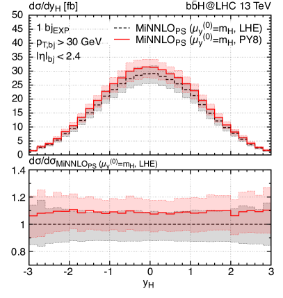
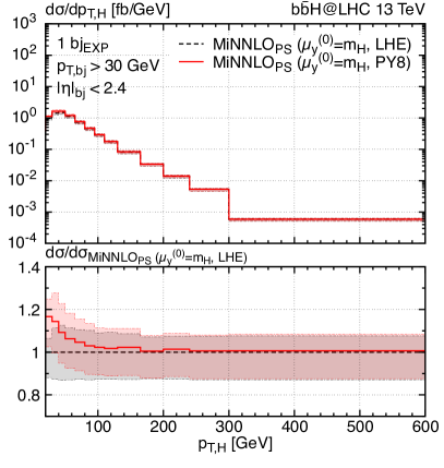
Figure 2: Comparison of MiNNLO_PS predictions in the 4FS at LHE (black, dashed) and including Pythia8 parton shower (red, solid) for the Higgs rapidity (left plot) and Higgs transverse momentum (right plot) with at least one $b$-jet.

5.3.2 Impact of the scale choice for the bottom Yukawa

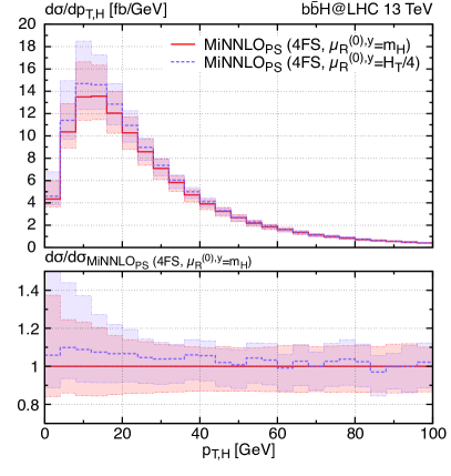
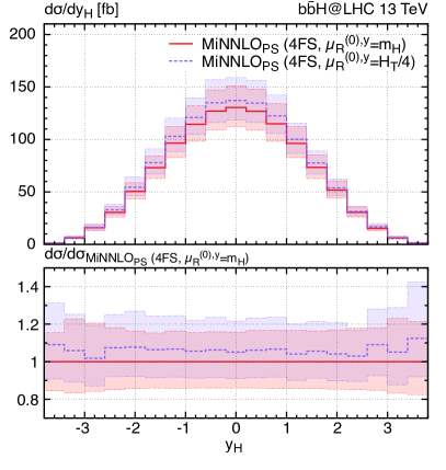
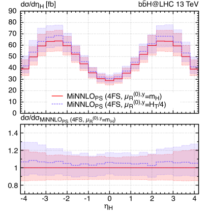
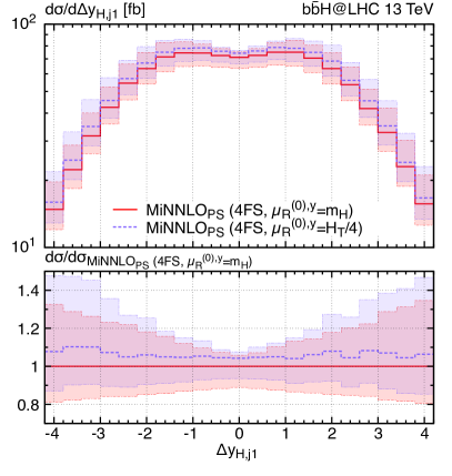
Figure 3: Comparison of two different scale choices ${\mu_{\text{R}}^{(0),y}}=m_{H}$ (red, solid) and ${\mu_{\text{R}}^{(0),y}}=H_{T}/4$ (violet, dashed) of the bottom-Yukawa coupling in MiNNLO_PS predictions for Higgs observables.

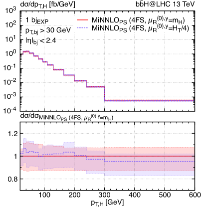
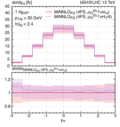
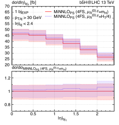
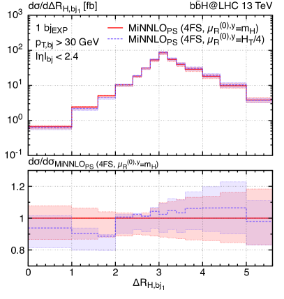
Figure 4: Comparison of two different scale choices ${\mu_{\text{R}}^{(0),y}}=m_{H}$ (red, solid) and ${\mu_{\text{R}}^{(0),y}}=H_{T}/4$ (violet, dashed) of the bottom-Yukawa coupling in MiNNLO_PS predictions $b$-jet observables.

We continue our phenomenological analysis by studying the impact of different scale choices for the bottom-Yukawa coupling at the differential level. To begin, we discuss the differential Higgs observables shown in figure 3. The first plot, shows the Higgs transverse-momentum spectrum, where the two MiNNLO_PS predictions are relatively close, especially in the high ${p_{\text{T,$H$}}}$ region. At low ${p_{\text{T,$H$}}}$ they differ up to 10%. The other plots in figure 3 show angular observables, including the Higgs rapidity ($y_{H}$) and pseudo-rapidity ($\eta_{H}$) distributions. Notice that these two distributions exhibit completely different shapes due to the Higgs boson being a massive particle. For massless particles, these observables coincide. However, the introduction of a mass creates a difference between the two distributions arising from the Jacobian factor

$$\frac{\mathop{}\!\mathrm{d}\sigma}{\mathop{}\!\mathrm{d}{\eta_{\text{H}}}}=\frac{{p_{\text{T,$H$}}}\cosh{\eta_{\text{H}}}}{\sqrt{{m_{\text{$H$}}}^{2}+{p_{\text{T,$H$}}}^{2}\cosh^{2}{\eta_{\text{H}}}}}\frac{\mathop{}\!\mathrm{d}\sigma}{\mathop{}\!\mathrm{d}{y_{\text{H}}}}.$$ (55)

Therefore, while a Higgs boson with zero pseudo-rapidity also has zero rapidity, the Jacobian factor alters the distribution near the peak, resulting in a maximum at a non-zero pseudo-rapidities. In both cases, the choice of the bottom-Yukawa coupling scale has a relatively small impact, inducing an effect of about 5%–10%, which is completely flat in these observables. The rapidity difference between the Higgs and the leading jet in the last plot of figure 3 shows exactly the same relative behaviour between the two scale choices.

Figure 4 shows differential cross sections with the $1\,bj_{\text{EXP}}$ requirement. The upper panel shows again the Higgs transverse momentum and rapidity distributions. The relative difference between the two scale choices is even smaller than in the fully inclusive case. However, the scale uncertainties are slightly reduced in the Higgs rapidity distribution when using the dynamical scale choice. In the first plot of the lower panel in figure 4, we show the absolute pseudo-rapidity spectrum of the leading $b$-jet ($|\eta|_{bj_{1}}$). Also here the two scale choices lead to fully consistent MiNNLO_PS predictions. Nevertheless, there is a very small difference in shape towards larger $|\eta|_{bj_{1}}$, although the effect remains below about $5\%$. In the last plot of figure 4, we show the distance between the Higgs boson and the leading $b$-jet in the $\eta$-$\phi$-plane ($\Delta R_{H,bj_{1}}$), where $\phi$ is the azimuthal angle and $\eta$ is the pseudo-rapidity in the laboratory frame. As expected, the distributions peaks around $\pi$. For $\Delta R_{H,bj_{1}}$ more pronounced shape differences between the two scale choices can be observed, especially below the peak, with effects up to 10%. Still, the predictions remain consistent within scale uncertainties.

While it has become customary to use the dynamical scale choice for the Yukawa coupling ${\mu_{\text{R}}^{(0),y}}=H_{T}/4$ in NLO(+PS) calculations in the 4FS, mostly because this results in a larger cross sections, as already noted in table 1, which are closer to the 5FS results, we adopt a fixed scale ${\mu_{\text{R}}^{(0),y}}=m_{H}$ as our default setting in the remainder of the paper. Not only does a setting of the scale of the Yukawa coupling of the order of the Higgs mass appear to be more appropriate, it also ensures consistency with the scale setting used for the bottom-Yukawa coupling in our 5FS predictions, enabling a more direct comparison at NNLO+PS level. Moreover, after having achieved NNLO QCD accuracy in both the 4FS and the 5FS, it is less relevant to tune the scales of these calculations in order for them to be in better agreement. Since the residual effects of changing the scale reduces significantly at higher orders, either scale choice is sufficient to achieve agreement between 4FS and 5FS predictions when NNLO QCD corrections are included.

5.3.3 Comparison with the NLO predictions

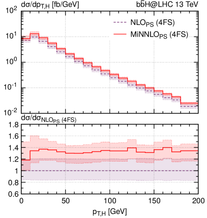
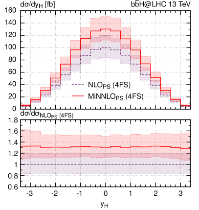
Figure 5: Comparison of NLO+PS (purple, dashed) and MiNNLO_PS (red, solid) predictions in the 4FS for Higgs observables.

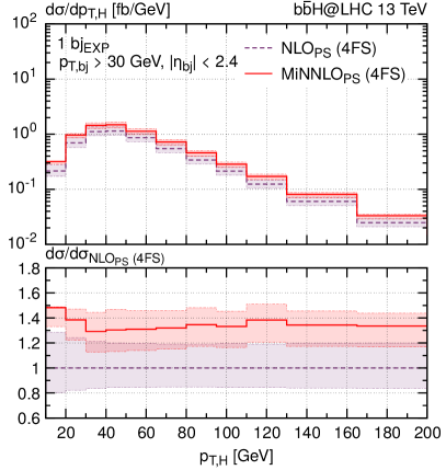
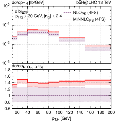
Figure 6: Comparison of NLO+PS (purple, dashed) and MiNNLO_PS (red, solid) predictions in the 4FS for the Higgs transverse-momentum spectrum with the requirement of at least one (left) or at least two $b$-jets (right).

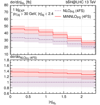
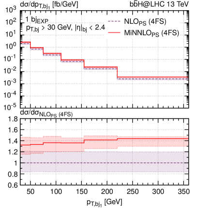
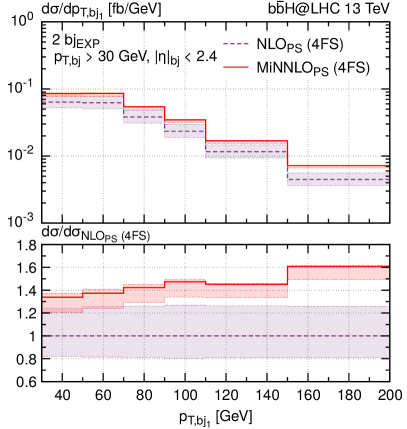
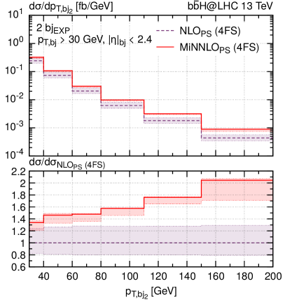
Figure 7: Comparison of NLO+PS (purple, dashed) and MiNNLO_PS (red, solid) predictions in the 4FS for the b-jet observables with the requirement of at least one (upper plots) or at least two $b$-jets (lower plots).

We now compare our MiNNLO_PS predictions with NLO+PS results to assess the relevance of NNLO QCD corrections in the 4FS. We can observe from figure 5 that NNLO corrections increase the NLO distributions in the Higgs transverse momentum and rapidity by about 30%, which shows a slight dependence at small transverse momenta, but is completely flat in the rapidity distribution. Indeed, we noticed the substantial effect of the NNLO corrections already at the level of the total inclusive cross section in table 1. The scale variations at NLO+PS do not cover the central MiNNLO_PS result and their bands barely touch. Due to the large corrections the scale uncertainties only reduce mildly, which can be considered as a good sign, as it makes the MiNNLO_PS scale uncertainties more robust.

Next, we stay with the transverse-momentum spectrum of the Higgs boson, but include a requirement on the minimal number of $b$-jets, shown in figure 6. We see that ${p_{\text{T,$H$}}}$ spectrum becomes broader with its peak shifting towards large values as more $b$-jets are required. Moreover, the relative correction at NNLO slightly increases to about $+40$% in both $b$-jet categories and still with a very mild dependence on the exact ${p_{\text{T,$H$}}}$ value. We also notice that the scale uncertainties are reduced in the MiNNLO_PS predictions compared to the NLO+PS ones, especially in the case where at least two identified $b$-jets are required. In that case, also the scale bands do not overlap any longer in several bins. This shows that NLO QCD accuracy in the 4FS is insufficient to provide reliable predictions for $b\bar{b}H$ production.

Finally, we consider $b$-jet observables in figure 7, where the effects become significantly more drastic for observables with at least two $b$-jets required. Looking at the upper plots in figure 7, which show the pseudo-rapidity and transverse-momentum distribution of the leading $b$-jet in the $\geq$1-$b$-jet category, we find similar results to before: NNLO corrections increase the NLO+PS cross section by 30%–40%, the dependence of these corrections on the observables is rather mild, and scale uncertainties decrease slightly, with largely overlapping bands, except at high transverse momenta of the leading $b$-jet. By, contrast in the leading and subleading $b$-jet transverse-momentum spectra with the requirement of at least two $b$-jets, there is a substantial increase in the NNLO corrections towards large transverse momenta, reaching up to a factor of two. As for the Higgs transverse-momentum spectrum in the $\geq$2-$b$-jet category, the MiNNLO_PS scale uncertainties are much smaller than the NLO+PS ones. Moreover, NLO+PS predictions completely fail in describing the cross section at large transverse momentum.

6 Comparison against the five-flavour scheme

This section aims at providing a thorough comparison of the MiNNLO_PS generators in the 4FS and 5FS at the differential level. In table 1, we have already compared the fully inclusive cross sections in both schemes. Besides distributions in the inclusive phase-space, we will study observables requiring at least one or two identified $b$-jets in the final state. In the 4FS, the experimental definition of $b$-jets, as described in section 5.1, can be directly applied, with infrared safety ensured by the finite bottom mass. However, in the 5FS, using an experimental definition of $b$-jets leads to IR-unsafe observables for massless bottom quarks. In principle, this can be adjusted in a parton-shower matched simulation by reshuffling the massless momenta to massive ones. Alternatively, an IR-safe definition of the jet flavour can be employed. Therefore, before comparing 4FS and 5FS results involving $b$-jets, we first explore different $b$-jet definitions within the MiNNLO_PS 5FS predictions in the following subsection.

6.1 Definition of $b$-jets in the massless case

In recent years, several attempts have been made to extend the anti-$k_{t}$ jet clustering algorithm to provide an infrared-and-collinear (IRC)-safe definition of heavy-flavour jets, when the respective quark is treated as massless. Various proposals have been recently formulated, including flavoured anti-$k_{t}$ Czakon:2022wam , Flavour Dressing Gauld:2023zlv and Interleaved Flavour Neutralisation Caola:2023wpj . See also refs. Buckley:2015gua ; Caletti:2022hnc ; Caletti:2022glq for alternative approaches to defining the jet flavour.

These algorithms address issues in flavour tagging, specifically the mismatch between virtual and real contributions when a flavour algorithm is applied to a theory prediction at fixed order in a massless scheme. This alignment is essential for ensuring an infrared-safe definition of observables involving flavoured jets. The potentially dangerous configurations involve either the splitting of a gluon into a bottom-quark pair within the same jet or soft wide-angle emissions of bottom quarks that are clustered with another hard parton. Both of these (potentially divergent) mechanisms alter the jet flavour if the algorithm is not properly defined.

These issues arise in the experimental approach for $b$-jet tagging, referred to as EXP in the following, as used in the previous section for our massive predictions. The challenge posed by a gluon splitting into a collinear bottom-quark pair that both end up in the same jet can be addressed with a straightforward solution: applying a modulo-2 condition on the number of bottom-flavoured quarks/hadrons within the same jet. This naive approach, labelled NAI in the following, classifies a jet as a $b$-jet if it contains only an odd number of bottom-flavoured quarks/hadrons. This solution does not solve the potential divergences from soft wide-angle emissions, but it captures the potentially more problematic and more frequent configurations. In addition, we consider in our analysis one of the more sophisticated IRC-safe approaches, precisely the Interleaved Flavour Neutralisation (IFN) Caola:2023wpj . The choices of the parameters in the definition of the neutralisation distance in IFN are the suggested ones: $\alpha=2$ and $\omega=1$. We developed a Fortran-C++ interface to enable the use of the Fastjet plugin within our Powheg analyses. This general-purpose interface is applicable to all processes implemented in Powheg.

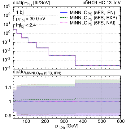
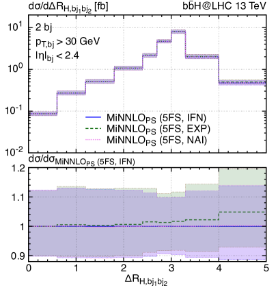
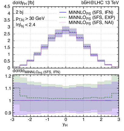
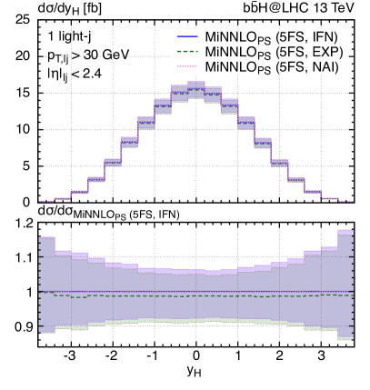
Figure 8: Comparison of different jet-flavour algorithms for $b$-jet predictions obtained with MiNNLO_PS in the 5FS for the EXP (green, dashed), NAI (pink, dotted) and IFN (blue, solid) $b$-jet definitions.

The MiNNLO_PS 5FS calculation is divided into several stages (corresponding to the ones in Powheg). Firstly, a fixed-order type prediction is obtained at the so-called stage-2 of Powheg. At this stage, the bottom quarks are massless, and we have verified that the EXP prediction depends on the technical cut-off present in the generation of the final-state radiation. The effect is small and visible only when the channel induced by bottom and anti-bottom quarks is selected. Although the effect is minor, IRC-unsafety is numerically evident due to the cut-off dependence. We, therefore, proceed with including the Powheg radiation at stage-4 according to the master formula in eq. (2) to produce LHE events, where the massless bottom quarks are mapped into massive states. Finally, we attach the shower radiation (that includes massive bottom quarks) to the LHE events for a physical description.

The massless-to-massive mapping introduces only power corrections in the quark mass, as long as the observable is infrared-safe and no collinear effects are screened by the mass. In addition, the Powheg matching is formally derived only for IRC-safe observables. In fact, in the formulation of the $\bar{B}$ function in Powheg in every event, the virtual and real contributions are combined into the same event weight. This combination cannot be split a posteriori by an IRC-unsafe $b$-tagging algorithm. As a result, the EXP or NAI $b$-jet tagging yield finite results in the MiNNLO_PS 5FS calculation (the same being true for any parton-shower matched prediction, e.g. any NLO+PS one). However, this poses the question whether such predictions can be trusted in providing a physical description of $b$-jet observables that are formally not IRC-safe in the 5FS or whether the finite results are an artificial remnant of the matching method. Although from a theoretical viewpoint it appears to us that only IRC-safe definitions, such as IFN, yield sensible results even in a matched parton-shower calculation for massless bottom quarks, 5FS predictions have been employed with the standard experimental definition for years in comparison to data, without being obviously flawed. Moreover, we have not found a way to unambiguously show numerically that matched parton-shower calculations fail to provide physical results in practice. On the contrary, we have not found any sensitivity to technical cut-offs so far that are present in the generation of LHE events at stage-4, unlike our findings for stage-2 discussed above. Therefore, we consider it beyond the scope of this paper to provide a final answer to this question, which we leave to future considerations.

Figure 8 shows a comparison of the three jet-flavour definitions for $b$-jet observables obtained with the MiNNLO_PS generator in the 5FS and including shower radiation. We note that we have selected the observables that show the largest differences. The first plot shows the transverse-momentum spectrum of the leading $b$-jet. Here, a difference between EXP and the other two definitions is evident in the large transverse-momentum region, while no differences between IFN and NAI are visible. This indicates that the differences of the EXP results are due to gluon splittings into collinear bottom quarks. A similar trend is observed for the rapidity separation between the Higgs and the dijet system formed by the two leading $b$-jets in the second plot in figure 8.

In the second row of figure 8 the Higgs rapidity spectrum is shown. In the left plot, we require the presence of at least two $b$-jets, while in the right plot, the event is accepted if it contains at least one jet that is not a $b$-jet, with the same requirements on the jet transverse momentum and rapidity. As expected, the IFN and NAI definitions lead to a smaller cross section compared to EXP in the two-$b$-jet region, as the flavour of some of the EXP $b$-jets is neutralised to ensure IRC safety. In contrast, due to number conservation, the EXP result, when at least one light jet is present, is smaller than the predictions by the other two definitions.

In general, the discrepancy between the experimental jet-flavour definition and IRC-safe algorithms like IFN is quite small in this process and well within scale uncertainties, as pathological configurations in the short-distance physics are suppressed by the bottom-quark PDFs. A small adjustment to the experimental approach, using the NAI definition, leads to predictions that are essentially identical to the theoretically robust IFN approach, with differences indistinguishable compared to the numerical uncertainties. Furthermore, we observe similar effects in the 4FS implementation using the different definitions of $b$-jets discussed here. We refer to ref. Gauld:SOON for more in-depth studies of different jet algorithms in the context of bottom-quark production. We continue with the flavour scheme comparison using the IFN tagging, noting that the NAI definition leads to indistinguishable results and even the EXP definition to very similar results.

6.2 Integrated results

Fiducial region	Generator	$\sigma_{\rm integrated}$ [fb]	Ratio to NLO+PS	Ratio to 5FS results
$pp\rightarrow H+0\,b$ jets	5FS NLO+PS	$583.(9)_{-22\%}^{+34\%}$	1.000	1.000
	5FS MiNNLOPS	$404.(2)_{-9.0\%}^{+5.9\%}$	0.692	1.000
	4FS NLO+PS	$285.(2)_{-25\%}^{+29\%}$	1.000	0.488
	4FS MiNNLOPS	$373.(9)_{-20\%}^{+22\%}$	1.311	0.925
$pp\rightarrow H+\geq 1\,b$ jets	5FS NLO+PS	$92.(7)_{-15\%}^{+27\%}$	1.000	1.000
	5FS MiNNLOPS	$104.(9)_{-8.7\%}^{+8.8\%}$	1.132	1.000
	4FS NLO+PS	$69.(4)_{-16\%}^{+21\%}$	1.000	0.749
	4FS MiNNLOPS	$92.(0)_{-12\%}^{+9.8\%}$	1.326	0.877
$pp\rightarrow H+\geq 2\,b$ jets	5FS NLO+PS	$4.8(9)_{-15\%}^{+27\%}$	1.000	1.000
	5FS MiNNLOPS	$7.6(4)_{-10\%}^{+11\%}$	1.562	1.000
	4FS NLO+PS	$4.4(9)_{-18\%}^{+25\%}$	1.000	0.991
	4FS MiNNLOPS	$6.3(9)_{-9.1\%}^{+1.5\%}$	1.423	0.836
$pp\rightarrow H+\geq 1\,\ell$ jets	5FS NLO+PS	$32.(8)_{-15\%}^{+27\%}$	1.000	1.000
	5FS MiNNLOPS	$53.(0)_{-7.6\%}^{+6.9\%}$	1.616	1.000
	4FS NLO+PS	$31.(4)_{-18\%}^{+26\%}$	1.000	0.987
	4FS MiNNLOPS	$38.(3)_{-12\%}^{+1.9\%}$	1.220	0.722

Table 2: Cross section rates for $b\bar{b}H$ production without any $b$-jets in the events ($pp\rightarrow H+0\,b$ jets) and with tagging of at least one $b$-jet ($pp\rightarrow H+\geq 1\,b$ jets), 2 $b$-jets ($pp\rightarrow H+\geq 2\,b$ jets), and at least one light jet ($pp\rightarrow H+\geq 1\,\ell$ jets) using the IFN jet-flavour algorithm.

We compare 4FS and 5FS predictions both at NLO+PS and NNLO+PS levels to assess the improvements in the consistency of the two schemes for the $b\bar{b}H$ process when higher-order corrections are included. The bottom-Yukawa coupling is evaluated at the scale of the Higgs mass throughout. We note that LO results are completely off and their uncertainties vastly underestimate the actual size of higher-order correction, which is why we refrain from including them in this comparison.

We start by studying fiducial rates with different requirements on $b$-jets and flavour-less jets, which are defined via the IFN jet-flavour algorithm, reported in table 2. Requiring at least one $b$-jet reduces the cross section by roughly a factor of 4–5, while requiring a second $b$-jet reduces the cross section by another factor of roughly 10. Compared to the cross section with at least one light flavour-less jet ($\ell$-jet), the cross section with at least one $b$-jet is three times larger. This is easy to understand, as the LO process contains two bottom quarks, while the light quarks are generated only through radiation at higher orders.

Looking at the column with the ratio to the NLO+PS predictions in table 2, one notices that NNLO corrections in either scheme are significant in all fiducial categories, ranging from 13% to 60%. Comparing the predictions in the two flavour schemes, we find that for the 0-$b$-jet and $\geq$1-b-jet cases, the cross sections at NLO+PS are not compatible with each other, whereas the MiNNLO_PS predictions improve the comparison substantially. The 0-$b$-jet rates agree within 8% and the $\geq$1-$b$-jet rates agree within 13%, fully compatible within the respective scale uncertainties at NNLO+PS.

Interestingly, we notice that for the $\geq$2-$b$-jet and $\geq$1-$\ell$-jet the NLO+PS results in 4FS and 5FS are very close, even closer than for the MiNNLO_PS predictions. These observables become successively less accurate in the 5FS, which at Born level does not feature bottom quarks in the hard matrix elements. Therefore, we conclude that the agreement at NLO+PS for these observables that are less accurate in the 5FS is completely accidental. Indeed, we will see when considering differential distributions in the next subsection that the shapes in 4FS and 5FS are vastly different at NLO+PS, which confirms the accidental agreement at the integrated cross-section level.

6.3 Differential results

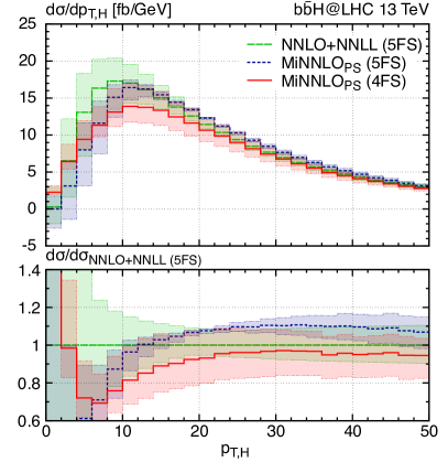
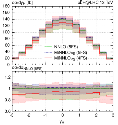
Figure 9: Comparison of the two MiNNLO_PS generators in the 5FS and 4FS with analytic results in the 5FS. The Higgs $p_{\text{T}}$ spectrum (left) is compared to the NNLO+NNLL predictions of ref. Harlander:2014hya using NNLO NNPDF 4.0 sets, while the Higgs rapidity spectrum (right) is compared with the NNLO fixed-order result of ref. Mondini:2021nck based on NNLO CT14 sets.

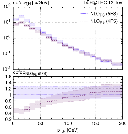
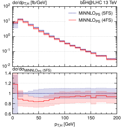
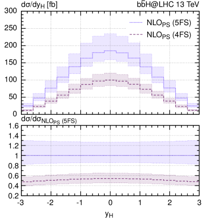
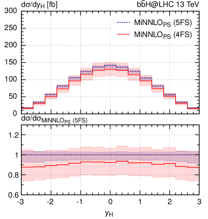
Figure 10: Comparison of 5FS and 4FS predictions at NLO+PS (left) and MiNNLO_PS (right) for Higgs observables with $\mu_{y}^{(0)}=m_{H}$ as fixed-scale of the Yukawa coupling.

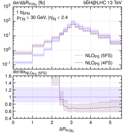
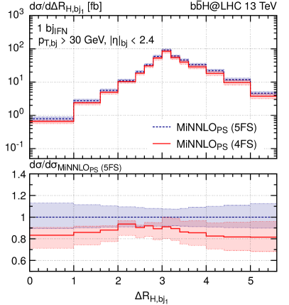
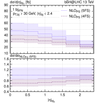
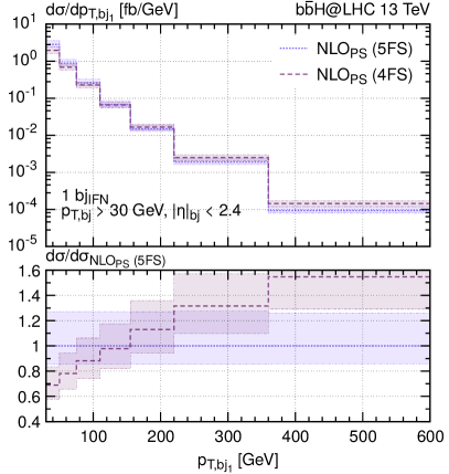
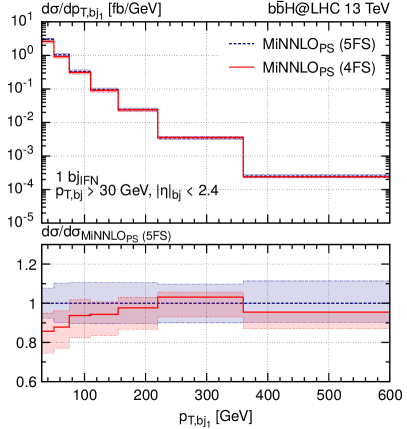
Figure 11: Comparison of 5FS and 4FS results at NLO+PS (left) and MiNNLO_PS (right) for observables with at least one $b$-jet defined using the IFN definition.

We begin the flavour-scheme comparison at the differential level by examining the distributions in Higgs transverse momentum and rapidity. Building upon the results presented in ref. Biello:2024vdh , which included comparisons with analytic predictions, we now incorporate our new 4FS NNLO+PS predictions in that comparison. In the left plot of figure 9, the MiNNLO_PS predictions for the Higgs transverse-momentum spectrum are compared with the NNLO+NNLL predictions from ref. Harlander:2014hya , obtained using the standard setup and the NNPDF 4.0 sets consistent with the respective flavour scheme. By and large, we observe that the three predictions are consistent within their respective uncertainties, although they exhibit some differences in their central values, especially at small transverse momenta. However, we expect that this region is now well described with the newly developed 4FS MiNNLO_PS calculation, which can be considered to be superior to the 5FS ones at small transverse momentum. This is because it includes power corrections in the bottom mass that become crucial around ${p_{\text{T,$H$}}}\sim m_{b}$. Also, the uncertainties of the 4FS MiNNLO_PS predictions appear to be more robust, since the 5FS MiNNLO_PS scale bands are smaller than the more accurate NNLO+NNLL prediction at small transverse momenta.

In the right plot of figure 9, the Higgs rapidity distribution from the two MiNNLO_PS generators are in full agreement with the NNLO fixed-order results from ref. Mondini:2021nck , which employs the NNLO set of the CT14 PDFs Dulat:2015mca . The agreement is particularly good in the central rapidity region.

We continue with the flavor-scheme comparison at NLO+PS and NNLO+PS. The first row of figure 10 shows the Higgs transverse-momentum distribution at NLO+PS (left) and NNLO+PS (right). At NLO+PS, a significant discrepancy is observed in the small ${p_{\text{T,$H$}}}$ region between the 4FS and 5FS predictions, while the MiNNLO_PS generators substantially improve the agreement between the two schemes in that region and achieve excellent consistency for ${p_{\text{T,$H$}}}>75$ GeV. In this range, the NNLO corrections in the 4FS are flat and well-contained within the scale uncertainties.

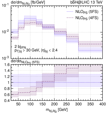
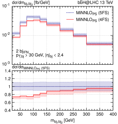
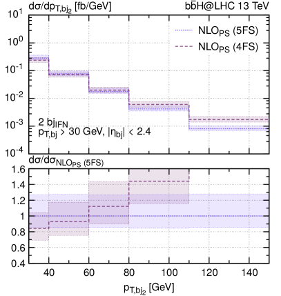
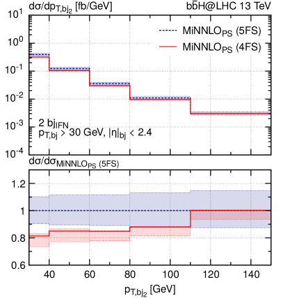
Figure 12: Comparison of 5FS and 4FS predictions at NLO+PS (left) and MiNNLO_PS (right) for the observables with at least 2 IFN $b$-jets.

The second row of figure 10 presents the Higgs rapidity spectrum, where the NLO+PS comparison (left panel) shows a substantial discrepancy between the two schemes, which differ by a factor of two or more, well outside the respective uncertainty bands. By contrast, the NNLO+PS predictions of the two MiNNLO_PS generators (right panel) are fully consistent within the uncertainty bands. These findings strongly indicate that the long-standing tension between the two schemes is fully resolved by the newly computed NNLO QCD corrections in the 4FS.

Figure 11 depicts observables for events tagged with one $b$-jet using the IFN definition. The separation in the $(\eta-\phi)$ plane between the Higgs and the leading $b$-jet reveals a substantial shape discrepancy between the NLO+PS generators (left panel). With the inclusion of NNLO corrections in the right panel, the agreement improves significantly. The shapes become much more similar and the uncertainty bands start overlapping. In the second row of figure 11, the pseudo-rapidity spectrum of the leading $b$-jet is in reasonable agreement within uncertainties both at NLO+PS and at NNLO+PS. However, in the latter case, the differences between the two schemes are reduced from about 25% to 10% and they show very similar shapes. The last two plots in figure 11 show the transverse-momentum spectrum of the hardest $b$-jet. Again the predictions in 4FS and 5FS, especially in terms of shape, are much closer for the MiNNLO_PS generators, with reduced uncertainty bands throughout.

We conclude this section by analysing observables based on events with at least two $b$-jets. The first row of figure 12 presents the invariant-mass distribution of the two leading $b$-jets. While the shapes at NLO+PS are vastly different for the two schemes, the agreement is clearly improved upon the inclusion of NNLO corrections, particularly in the high-mass region. However, notable discrepancies up to 30% persist below 150 GeV. Despite the clear improvement at NNLO+PS the difference between the two schemes is not covered by the respective scale uncertainties in that region. We emphasise that for these observables the 5FS prediction achieves effectively only LO+PS accuracy, while the 4FS provides an NNLO+PS description. This can be seen from the larger uncertainty bands in the 5FS. The plots in the lower panel of the same figure display the transverse-momentum spectrum of the subleading $b$-jet, where we observe a very similar behaviour as for the previous observable.

Regarding the scale variation, we observe that the 4FS NNLO+PS results yield a significantly more conservative uncertainty than the 5FS ones for inclusive predictions. This behaviour, shown in figure 10, is consistent with the trend seen in other processes where bottom quarks appear in the final state of the hard scattering. When requiring at least one $b$-jet, the two MiNNLO_PS predictions exhibit similar scale-variation bands, as can be seen in figure 11. In contrast, figure 12 displays a narrower uncertainty band for the 4FS prediction compared to the 5FS one, reflecting the higher accuracy of the massive scheme, while the massless scheme is only LO+PS accurate.

7 Background for $HH$ searches in the $2b2\gamma$ channel

In this section, we examine a potential application of our novel MiNNLO_PS generator in the 4FS to model the $b\bar{b}H$ background to the di-Higgs ($HH$) signal. For an illustrative $HH$ search, we consider the $2b2\gamma$ decay mode, in which one Higgs boson decays into $b$-quarks and the other into photons. Ref. Manzoni:2023qaf investigates the impact of the $b\bar{b}H$ background on $HH$ searches, considering both $y_{b}^{2}$ and $y_{t}^{2}$ contributions at NLO+PS within the MG5_aMC@NLO framework Alwall:2014hca . Specifically, they analysed $b\bar{b}H$ production with the decay $H\rightarrow\gamma\gamma$ and compared both the total and various fiducial rates at NLO against the $HH$ signal Heinrich:2017kxx . The findings of ref. Manzoni:2023qaf reveal that NLO QCD corrections are substantial and essential for obtaining an accurate prediction of the $b\bar{b}H$ background. Corrections are notably larger for the $y_{t}^{2}$ contributions, enhancing the leading-order (LO) prediction by approximately $+150\%$, while the impact on the $y_{b}^{2}$ terms is around $+50\%$. The residual uncertainties, arising from variations in renormalisation and factorisation scale, are about $+50\%$ and $-30\%$ for the combined $y_{b}^{2}$ and $y_{t}^{2}$ contributions to the $b\bar{b}H$ cross section. The study in ref. Manzoni:2023qaf also suggests that current limits on $\sigma^{HH}_{\rm SM}$ will improve by a few percent in the $2b2\gamma$ final state when modelling the $b\bar{b}H$ background at NLO+PS, and that HL-LHC constraints on $\sigma^{HH}_{\rm SM}$ and the $HH$ discovery significance could improve by 5%. We note that the estimated improvements are even larger in the $2b2\tau$ channel Manzoni:2023qaf .

By the end of HL-LHC, Higgs pair production is anticipated to be observed at nearly five standard deviations. As a result, accurate modelling of the $b\bar{b}H$ background in appropriate fiducial phase space regions is critical for improving sensitivity to the $HH$ signal. Given the importance of precise $b\bar{b}H$ background modelling for $HH$ searches, we aim to improve the accuracy of this background in the $y_{b}^{2}$ channel. Specifically, we provide novel NNLO predictions for $b\bar{b}H$ production proportional to $y_{b}^{2}$, including the decay $H\rightarrow\gamma\gamma$, using our new MiNNLO_PS generator in the 4FS. We employ Pythia8 Bierlich:2022pfr to model the Higgs boson decay to two photons in the narrow-width approximation. The branching fraction is taken to be ${\rm BR}(H\rightarrow\gamma\gamma)=0.227\%$ LHCHiggsCrossSectionWorkingGroup:2016ypw .

We use the same setup as described in section 5.1, except for the phase-space cuts on jets, where we follow the approach given in ref. ATLAS:2021ifb . Specifically, we consider anti-$k_{T}$ jets Cacciari:2008gp with a radius parameter $R=0.4$ as implemented in FastJet Cacciari:2011ma . Bottom-flavored jets (b-jets) are defined according to the EXP definition used previously. In this theoretical study, the criteria for selecting jets are as follows:

$$p_{T}(j)>25,\mathrm{GeV}\qquad{\rm and}\qquad|\eta(j)|<2.5\,.$$ (56)

We define the $HH$ signal region by selecting events that contain exactly two $b$-jets and two photons, with QED showering turned off in the simulations. We also impose a cut on the invariant mass of the $b$-jet pair:

$$80\,\mathrm{GeV}<m(b_{1},b_{2})<140\,\mathrm{GeV}\,.$$ (57)

The photon pair is required to meet the following conditions:

$$105\,\mathrm{GeV}<m(\gamma_{1},\gamma_{2})<160\,\mathrm{GeV},\quad|\eta(\gamma_{i})|<2.37,\quad\frac{p_{T}(\gamma_{1})}{m(\gamma_{1},\gamma_{2})}>0.35,\quad\frac{p_{T}(\gamma_{2})}{m(\gamma_{1},\gamma_{2})}>0.25\,.$$ (58)

Since the Higgs boson is produced on-shell in our generator and Pythia8 handles the decay without including QED shower effects, the narrow-width approximation trivially satisfies the condition $m(\gamma_{1},\gamma_{2})-m_{H}=\mathcal{O}(\Gamma_{H})$.

In addition to the aforementioned cuts, hereafter referred to as fiducial cuts, we introduce the following quantities for the invariant mass of the diphoton plus b-tagged jets system:

$$m_{2b2\gamma}=m(b_{1},b_{2},\gamma_{1},\gamma_{2})\,,$$ (59)

and

$$m_{2b2\gamma}^{\star}=m_{2b2\gamma}-m(b_{1},b_{2})-m(\gamma_{1},\gamma_{2})+2m_{H}\,.$$ (60)

We then consider three different event categories by imposing the following cuts on $m_{2b2\gamma}^{\star}$:

$$m_{2b2\gamma}^{\star}<\infty,\qquad m_{2b2\gamma}^{\star}<500\,\mathrm{GeV},\qquad m_{2b2\gamma}^{\star}<350\,\mathrm{GeV}\,.$$ (61)

The first condition represents the fiducial cuts, while the other two impose progressively stricter requirements on $m_{2b2\gamma}^{\star}$.

7.1 Inclusive predictions

Fiducial region	4FS NLO+PS	4FS MiNNLOPS	Ratio to NLO+PS
No cut	$805_{-16\%}^{+20\%}$	$1056_{-14\%}^{+16\%}$	1.312
Fid. cuts	$3.56_{-18\%}^{+24\%}$	$5.10_{-9.5\%}^{+2.1\%}$	1.432
Fid. cuts + $m_{2b2\gamma}^{\star}<500\,\mathrm{GeV}$	$3.50_{-18\%}^{+24\%}$	$5.04_{-9.6\%}^{+2.4\%}$	1.440
Fid. cuts + $m_{2b2\gamma}^{\star}<350\,\mathrm{GeV}$	$3.01_{-18\%}^{+25\%}$	$4.38_{-9.7\%}^{+2.8\%}$	1.455

Table 3: Cross sections in ab for the $y_{b}^{2}$ contribution to $pp\rightarrow b\bar{b}H$ with $H\rightarrow\gamma\gamma$ decay.

We present the total and fiducial rates for $b\bar{b}H$ production in the 4FS, including the decay $H\rightarrow\gamma\gamma$, at NLO+PS and for MiNNLO_PS in table 3. The fiducial cuts, which correspond to the $HH$ signal region, are defined according to the definitions in eqs. (56)–(58), and with the additional constraints on $m_{2b2\gamma}^{\star}$ given in eq. (61). For the total inclusive cross section, the NNLO corrections yield a $+30\%$ increase with respect to the NLO result, with scale uncertainties of about $+16\%$ and $-14\%$, which is in line with the inclusive results presented in table 1. In the fiducial categories, the NNLO corrections contribute about $+40\%$ with respect to the NLO prediction, while scale uncertainties are significantly reduced to $+2\%$ and $-9\%$. The fiducial cuts significantly reduce the $b\bar{b}H$ background, lowering the cross section by roughly a factor of 100 compared to the total inclusive cross section. Imposing additional constraints on $m_{2b2\gamma}^{\star}$ further lowers the cross section, with a reduction of approximately $1\%$ for $m_{2b2\gamma}^{\star}<500\,$GeV and $14\%$ for $m_{2b2\gamma}^{\star}<350\,$ GeV, respectively. However, in all categories the $y_{b}^{2}$ contribution to the $b\bar{b}H$ cross section remains at the same order as the $HH$ signal cross section, making its accurate modelling so crucial. Given the large corrections in the $y_{b}^{2}$ contribution to the $b\bar{b}H$ background, our analysis clearly shows the relevance of including NNLO terms in this context.

7.2 Differential distributions

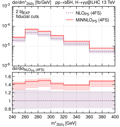
Figure 13: Comparison of the $m_{2b2\gamma}^{\star}{}$ distribution at NLO+PS and MiNNLO_PS including fiducial cuts.

Finally, we study differential distributions, which provide deeper insights into the kinematics of the $b\bar{b}H$ process in the $HH$ signal region. These results could be valuable for understanding which phase-space regions might help reduce the $b\bar{b}H$ background in $HH$ measurements or, more broadly, for assessing how different cuts affect the $b\bar{b}H$ process. We start with the $m_{2b2\gamma}^{\star}{}$ distribution in figure 13 within the phase space defined by the fiducial cuts. Both the NLO+PS and MiNNLO_PS spectra show a suppression as we go to higher values of $m_{2b2\gamma}^{\star}{}$. Comparing the NLO and NNLO predictions, we observe that the NNLO corrections are positive and substantial, with an enhancement of about $40\%$–$50\%$ over the considered $m_{2b2\gamma}^{\star}{}$ range. There is only a slight shift in the distribution shape at low $m_{2b2\gamma}^{\star}{}$. Scale uncertainties are significantly at NNLO+PS, with no overlap between the NLO and MiNNLO_PS uncertainty bands, highlighting the importance of the newly calculated NNLO corrections for this process.

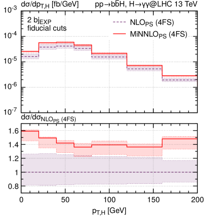
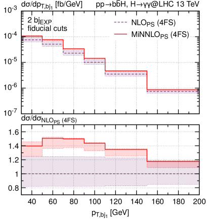
Figure 14: Comparison of the transverse-momentum spectrum of the Higgs boson reconstructed from the two photons (left) and of the leading $b$-jet (right) at NLO+PS and MiNNLO_PS including fiducial cuts.

Next, we analyse the transverse-momentum distributions for the Higgs boson, reconstructed from the two photons, shown in the left plot of figure 14, and for the leading $b$-jet in the right plot of figure 14, with fiducial baseline selection cuts applied. The NNLO corrections show an enhancement of $40\%$–$50\%$ across the spectrum except for large ${p_{\text{T,$bj_{1}$}}}$. Additionally, there is minimal overlap between the NLO and MiNNLO_PS uncertainty bands, emphasizing the critical role of including NNLO corrections. The scale uncertainties are significantly reduced for both observables at NNLO+PS, especially for the ${p_{\text{T,$bj_{1}$}}}$ distribution, where the reduction in scale uncertainty is most pronounced.

8 Conclusions

In this work, we have presented a novel NNLO+PS event generator for the production of a Higgs boson in association with a bottom-quark pair induced by the bottom-Yukawa coupling. The calculation has been performed in the flavour scheme with four massless quark flavours and massive bottom and top quarks. Our results represent the first computation of NNLO QCD corrections to this process. Moreover, this is only the second process of such complexity, namely with a heavy-quark pair and an extra colour singlet particle in the final state, for which NNLO QCD corrections are matched with parton showers.

The present computation has been rendered feasible by two major developments. Firstly, we incorporated in the MiNNLO_PS method all the essential components for computing processes that involve a heavy-quark pair in association with a colour singlet in the final state as well as an overall scale-dependent Yukawa coupling. Secondly, the major bottleneck on the amplitude side is posed by the complexity of the double-virtual contribution, which we resolved by taking the limit of a small bottom mass, i.e. neglecting only power-suppressed terms in the bottom-quark mass while keeping all other contributions in the NNLO+PS calculation exact. We stress that this is an excellent approximation for $b\bar{b}H$ production at LHC energies, since power-suppressed terms in the bottom-quark mass are expected to be sufficiently small. Indeed, we have confirmed the high quality of this approximation explicitly at NLO+PS.

We have employed our new $b\bar{b}H$ generator in an extensive phenomenological analysis, highlighting the importance of NNLO corrections and parton-shower matching for this process. The NNLO corrections in the four-flavour scheme are quite sizeable and consistently enhance the $b\bar{b}H$ cross section by about 30%, which are not fully captured by the scale variations of the NLO+PS predictions. Differentially these effects can be significantly enhanced, reaching NNLO corrections up to 100% in some distributions.

We have compared our NNLO+PS predictions in the four-flavour scheme with massive bottom quarks against the previous NNLO+PS calculation in the five-flavour scheme from ref. Biello:2024vdh . Fixed-order results in the five-flavour scheme require an IR-safe algorithm for the identification of the bottom-flavoured jets, and a certain sensitivity could also be present in calculations matched to parton showers. To study this, we have considered both the standard experimental approach to tag bottom-quark jets and the Interleaved Flavour Neutralisation definition of bottom-quark jets Caola:2023wpj . However, we found (both for the five- and the four-flavour scheme calculations) that the impact of such an IR-safe algorithm is minor in practice. Only the removal of $g\rightarrow b\bar{b}$ splittings, i.e. identifying a jet including a $b\bar{b}$ pair not as a bottom-quark jet, has a noticeable impact on the predictions, simply because these respective topologies are removed.

A major result of our work is that the NNLO corrections in the four-flavour scheme, computed here for the first time, solve the long-standing discrepancy between lower-order predictions in the two schemes. Both MiNNLO_PS generators describe Higgs observables and predictions with at least one identified bottom-flavour jet consistently within their respective uncertainties. Notably, the four-flavour scheme calculation delivers more precise predictions for events with identified bottom-quark jets, especially in configurations with at least one of them, where the 5FS NNLO+PS prediction is less accurate.

We have also presented an application of our NNLO+PS generator to estimate the $b\bar{b}H$ background in di-Higgs searches for the signature where one Higgs boson decays into bottom quarks and the other into photons. For typical event categories of the $HH$ signal in the $b\bar{b}\gamma\gamma$ final state we have found that the $b\bar{b}H$ background proportional to the bottom-quark Yukawa coupling increases by 30%–50% upon inclusion of NNLO QCD corrections. This provides an important example of the phenomenological impact of the developed $b\bar{b}H$ generator on future $HH$ measurements.

We reckon that our new $b\bar{b}H$ MiNNLO_PS generator will have important implications on various aspects of LHC phenomenology and that it will be a very useful tool for the experimental collaborations at the LHC. We plan to make the associated code publicly available within the Powheg-Box-Res framework shortly, and the numerical results, events and code are available upon request.

With the completion of the two NNLO+PS generators in the four- and five-flavour schemes, it will be interesting to consider their consistent combination, since each scheme describes different contributions in bottom-quark mass more accurately. Thus, developing a unified approach that combines the two schemes at NNLO+PS level, which has never been done before, could achieve unprecedented precision in the description of associated $b\bar{b}H$ production and also provide a pathway to apply such approach to similar processes in the future. Additionally, our calculation provides the basis to develop MiNNLO_PS generators for processes with lighter quark flavours in the final state, such as Higgs production in association with charm quarks in the final state. Not least, the gluon-fusion component to $b\bar{b}H$ production proportional to the top-Yukawa coupling could be considered with similar techniques. All these developments are left for future work.

9 Acknowledgments

We are grateful to Chiara Savoini for performing cross-checks on the numerical implementation of the double-virtual correction. We acknowledge the OpenLoops authors, particularly Federico Buccioni, for providing a suitable set of amplitudes. We also thank Vasily Sotnikov and Simone Zoia for discussions during the course of this work. All simulations presented here were carried out using the Max Planck Computing and Data Facility (MPCDF) in Garching.

Appendix A Ingredients for the two-loop approximation

In this appendix, we provide the momentum mapping and the massification factors that are used for the massification procedure of the two-loop contribution described in section 4.1.

A.1 Momentum mapping

The phase-space points $\{p_{i}\}$ in Powheg assumes massive bottom quarks,

$$c(p_{1})\bar{c}(p_{2})\rightarrow b(p_{3})\bar{b}(p_{4})H(p_{5})\,,$$ (62)

with $p_{3}^{2}=p_{4}^{2}=m_{b}^{2}$ and $c=q,\bar{q},g$. However, the approximation requires the evaluation of the amplitudes with massless bottom quarks by using a suitable set of momenta,

$$c(\tilde{p}_{1})\bar{c}(\tilde{p}_{2})\rightarrow b(\tilde{p}_{3})\bar{b}(\tilde{p}_{4})H(\tilde{p}_{5})$$ (63)

where $\tilde{p}_{3}^{2}=\tilde{p}_{4}^{2}=0$. We define a mapping $\{p_{i}\}\rightarrow\{\tilde{p}_{i}\}$ that introduces only power-corrections $\mathcal{O}(m_{b}/\mu_{h})$ in the redefinition of the momenta and preserve the kinematics of the Higgs state, i.e. $\tilde{p}_{5}=p_{5}$. In the quark-induced channel, we can easily preserve also the momenta of the incoming partons. These conditions imply that $p_{3}+p_{4}=\tilde{p}_{3}+\tilde{p}_{4}$. Therefore also the invariant mass of the bottom-quark pair is preserved,

$$m_{b\bar{b}}=(p_{3}+p_{4})^{2}=(\tilde{p}_{3}+\tilde{p}_{4})^{2}\,,$$ (64)

as an invariant of the mapping. Therefore, by introducing the light-cone factors,

$$\rho_{\pm}=\frac{1\pm\rho}{2\rho},\,\rho=\sqrt{1-\frac{4m_{b}^{2}}{m_{b\bar{b}}^{2}}}\,,$$ (65)

we define the massless momenta

$$\tilde{p}_{3}=\rho_{+}p_{3}-\rho_{-}p_{4}\,,$$ (66)

$$\tilde{p}_{4}=\rho_{+}p_{4}-\rho_{-}p_{3}\,,$$ (67)

which tend to $p_{3}$ and $p_{4}$, respectively, in the limit $m_{b}\rightarrow 0$. If we were to apply the previous mapping to subprocesses with initial state gluons, an initial-final collinear divergence could appear, as also observed in Mazzitelli:2024ura ; Devoto:2024nhl . Therefore, in the gluon channel, we have adopted a different modification of the bottom-quark momenta,

$$\tilde{p}_{j}=p_{j}+\left(\sqrt{1-\frac{m_{b}^{2}n_{j}^{2}}{\left(p_{j}\cdot n_{j}\right)^{2}}}-1\right)\frac{p_{j}\cdot n_{j}}{n_{j}^{2}}n_{j}\,\hskip 28.45274pt\text{with }j\in\{3,4\}\,,$$ (68)

where we have introduced two vectors, transverse to both the initial-state momenta,

$$n_{j}=p_{j}-p_{1}\frac{p_{2}\cdot p_{j}}{p_{1}\cdot p_{2}}-p_{2}\frac{p_{1}\cdot p_{j}}{p_{1}\cdot p_{2}}\,.$$ (69)

In order to restore the momentum conservation, we have used an initial-state recoil, such that

$$\tilde{p}_{1}+\tilde{p}_{2}=p_{1}+p_{2}-\left(\tilde{p}_{3}+\tilde{p}_{4}-p_{3}-p_{4}\right)\,.$$ (70)

We stress that the Higgs kinematics is also preserved in the gluon channel with the previous choices.

A.2 Massification factors

The coefficients of the factor $\mathcal{\bar{F}}$ up to $\mathcal{O}(\alpha_{s}^{2})$ in eq. (45) are presented in ref. Mazzitelli:2024ura with the needed corrections from heavy-quark loops. For completeness, we report the first-order coefficient as follows,

$$\bar{\mathcal{F}}_{c\bar{c}}^{(1)} =2C_{\mathrm{F}}\leavevmode\nobreak\ \ell_{b}^{2}+C_{\mathrm{F}}\leavevmode\nobreak\ \ell_{b}+C_{\mathrm{F}}\left(2+\frac{\pi^{2}}{12}\right)\leavevmode\nobreak\ +\leavevmode\nobreak\ n_{h}\bar{\mathcal{F}}^{(1)}_{n_{h},c\bar{c}}\,,$$ (71)

with

$$\bar{\mathcal{F}}^{(1)}_{n_{h},q\bar{q}}=0\,,\quad\bar{\mathcal{F}}^{(1)}_{n_{h},gg}=-\frac{2}{3}\leavevmode\nobreak\ \ell_{b}\,,$$ (72)

while the second-order term reads as

$$\bar{\mathcal{F}}_{c\bar{c}}^{(2)} =2C_{\mathrm{F}}^{2}\leavevmode\nobreak\ \ell_{b}^{4}+\leavevmode\nobreak\ \ell_{b}^{3}\left(\frac{22}{9}C_{\mathrm{A}}C_{\mathrm{F}}+2C_{\mathrm{F}}^{2}-\frac{4}{9}C_{\mathrm{F}}n_{l}\right)+$$

$$\leavevmode\nobreak\ \ell_{b}^{2} \left(C_{\mathrm{A}}C_{\mathrm{F}}\left(\frac{167}{18}-\frac{\pi^{2}}{3}\right)+C_{\mathrm{F}}^{2}\left(\frac{9}{2}+\frac{\pi^{2}}{6}\right)-\frac{13}{9}C_{\mathrm{F}}n_{l}\right)+$$

$$\leavevmode\nobreak\ \ell_{b} \left(C_{\mathrm{A}}C_{\mathrm{F}}\left(\frac{1165}{108}+\frac{14}{9}\pi^{2}-15\zeta_{3}\right)+C_{\mathrm{F}}^{2}\left(\frac{11}{4}-\frac{11}{12}\pi^{2}+12\zeta_{3}\right)-C_{\mathrm{F}}n_{l}\left(\frac{77}{54}+\frac{2}{9}\pi^{2}\right)\right)+$$

$$C_{\mathrm{F}}^{2}\left(\frac{241}{32}-\frac{163}{1440}\pi^{4}+\pi^{2}\left(\frac{13}{12}-2\log(2)\right)-\frac{3}{2}\zeta_{3}\right)+$$

$$C_{\mathrm{A}}C_{\mathrm{F}}\left(\frac{12877}{2592}-\frac{47}{720}\pi^{4}+\pi^{2}\left(\frac{323}{432}+\log(2)\right)+\frac{89}{36}\zeta_{3}\right)-$$

$$C_{\mathrm{F}}\,n_{l}\left(\frac{1541}{1296}+\frac{37}{216}\pi^{2}+\frac{13}{18}\zeta_{3}\right)\;+\;n_{h}\,\bar{\mathcal{F}}^{(2)}_{n_{h},c\bar{c}}\,,$$ (73)

with

$$\bar{\mathcal{F}}^{(2)}_{n_{h},q\bar{q}}=-\frac{20}{9}\leavevmode\nobreak\ \ell_{b}^{3}C_{\mathrm{F}}+\frac{32}{9}\leavevmode\nobreak\ \ell_{b}^{2}C_{\mathrm{F}}+\leavevmode\nobreak\ \ell_{b}C_{\mathrm{F}}\left(-\frac{157}{27}-\frac{7}{18}\pi^{2}\right)+C_{\mathrm{F}}\left(\frac{1933}{324}-\frac{13}{108}\pi^{2}-\frac{7}{9}\zeta_{3}\right),$$ (74)

$$\bar{\mathcal{F}}^{(2)}_{n_{h},gg}=\leavevmode\nobreak\ \ell_{b}^{3}\left(-\frac{4}{9}C_{\mathrm{A}}-\frac{28}{9}C_{\mathrm{F}}\right)+\leavevmode\nobreak\ \ell_{b}^{2}\left(\frac{10}{9}C_{\mathrm{A}}+\frac{7}{9}C_{\mathrm{F}}\right)+$$

$$\leavevmode\nobreak\ \ell_{b}\left(C_{\mathrm{F}}\left(-\frac{319}{54}-\frac{5}{18}\pi^{2}\right)+C_{\mathrm{A}}\left(-\frac{92}{27}+\frac{\pi^{2}}{18}\right)\right)+$$

$$\,C_{\mathrm{A}}\left(\frac{179}{108}-\frac{5}{216}\pi^{2}-\frac{7}{18}\zeta_{3}\right)+C_{\mathrm{F}}\left(\frac{2677}{1296}-\frac{41}{216}\pi^{2}-\frac{\zeta_{3}}{18}\right)\leavevmode\nobreak\ +\leavevmode\nobreak\ \frac{4}{9}n_{h}\leavevmode\nobreak\ \ell_{b}^{2}\,.$$ (75)

Here, the number $n_{l}=4$ represents the light flavours in the 4FS calculation, while $n_{h}=1$ is the number of quarks running in the loops that we want to promote to a massive state. The $n_{h}$ part is the novel contribution from the massification factors of the generalised massification approach in eq. (42) compared to the procedure encoded in eq. (40). The logarithmic contributions are expressed as $\leavevmode\nobreak\ \ell_{b}=-\log\left(m_{b}/\mu_{R}\right)$ for compactness.

The non-trivial coefficient of the soft function in eq. (46) is

$$\mathcal{S}^{(2)} =n_{h}\left(-\frac{2}{3}\leavevmode\nobreak\ \ell_{b}^{2}+\frac{10}{9}\leavevmode\nobreak\ \ell_{b}-\frac{14}{27}\right)\,.$$ (76)

References

- (1) ATLAS Collaboration, The ATLAS experiment at the CERN Large Hadron Collider, JINST 3 (2008) S08003.
- (2) CMS Collaboration, The CMS experiment at the CERN LHC, JINST 3 (2008) S08004.
- (3) ATLAS Collaboration, Observation of a new particle in the search for the standard model Higgs boson with the ATLAS detector at the LHC, Phys. Lett. B 716 (2012) 1, [1207.7214].
- (4) CMS Collaboration, Observation of a new boson at a mass of 125 GeV with the CMS experiment at the LHC, Phys. Lett. B 716 (2012) 30, [1207.7235].
- (5) CMS Collaboration, Observation of a new boson with mass near 125 GeV in collisions at = 7 and 8 TeV, JHEP 06 (2013) 081, [1303.4571].
- (6) ATLAS Collaboration, A detailed map of Higgs boson interactions by the ATLAS experiment ten years after the discovery, Nature 607 (2022) 52, [2207.00092].
- (7) CMS Collaboration, A portrait of the Higgs boson by the CMS experiment ten years after the discovery, Nature 607 (2022) 60, [2207.00043].
- (8) ATLAS collaboration, A detailed map of Higgs boson interactions by the ATLAS experiment ten years after the discovery, Nature 607 (2022) 52–59, [2207.00092].
- (9) CMS collaboration, A. Tumasyan et al., A portrait of the Higgs boson by the CMS experiment ten years after the discovery, Nature 607 (2022) 60–68, [2207.00043].
- (10) LHC Higgs Cross Section Working Group collaboration, D. de Florian et al., Handbook of LHC Higgs Cross Sections: 4. Deciphering the Nature of the Higgs Sector, 1610.07922.
- (11) ATLAS Collaboration, Observation of Higgs boson production in association with a top quark pair at the LHC with the ATLAS detector, Phys. Lett. B 784 (2018) 173, [1806.00425].
- (12) CMS Collaboration, Observation of H production, Phys. Rev. Lett. 120 (2018) 231801, [1804.02610].
- (13) D. Pagani, H.-S. Shao and M. Zaro, RIP : how other Higgs production modes conspire to kill a rare signal at the LHC, JHEP 11 (2020) 036, [2005.10277].
- (14) F. Bishara, U. Haisch, P. F. Monni and E. Re, Constraining light-quark Yukawa couplings from Higgs distributions, Phys. Rev. Lett. 118 (2017) 121801, [1606.09253].
- (15) J. Alison et al., Higgs boson potential at colliders: Status and perspectives, Rev. Phys. 5 (2020) 100045, [1910.00012].
- (16) S. Manzoni, E. Mazzeo, J. Mazzitelli, M. Wiesemann and M. Zaro, Taming a leading theoretical uncertainty in HH measurements via accurate simulations for production, JHEP 09 (2023) 179, [2307.09992].
- (17) ATLAS collaboration, HL-LHC prospects for the measurement of Higgs boson pair production in the final state and combination with the and final states at the ATLAS experiment, .
- (18) G. Das, Higgs boson rapidity distribution in bottom annihilation at NNLL and beyond, Phys. Rev. D 108 (2023) 094028, [2306.04561].
- (19) D. Dicus, T. Stelzer, Z. Sullivan and S. Willenbrock, Higgs boson production in association with bottom quarks at next-to-leading order, Phys.Rev. D59 (1999) 094016, [hep-ph/9811492].
- (20) C. Balazs, H.-J. He and C. Yuan, QCD corrections to scalar production via heavy quark fusion at hadron colliders, Phys.Rev. D60 (1999) 114001, [hep-ph/9812263].
- (21) R. V. Harlander and W. B. Kilgore, Higgs boson production in bottom quark fusion at next-to-next-to leading order, Phys.Rev. D68 (2003) 013001, [hep-ph/0304035].
- (22) J. M. Campbell, R. K. Ellis, F. Maltoni and S. Willenbrock, Higgs-Boson production in association with a single bottom quark, Phys.Rev. D67 (2003) 095002, [hep-ph/0204093].
- (23) R. V. Harlander, K. J. Ozeren and M. Wiesemann, Higgs plus jet production in bottom quark annihilation at next-to-leading order, Phys. Lett. B693 (2010) 269–273, [1007.5411].
- (24) K. J. Ozeren, Analytic Results for Higgs Production in Bottom Fusion, JHEP 1011 (2010) 084, [1010.2977].
- (25) R. Harlander and M. Wiesemann, Jet-veto in bottom-quark induced Higgs production at next-to-next-to-leading order, JHEP 1204 (2012) 066, [1111.2182].
- (26) S. Buhler, F. Herzog, A. Lazopoulos and R. Muller, The fully differential hadronic production of a Higgs boson via bottom quark fusion at NNLO, JHEP 1207 (2012) 115, [1204.4415].
- (27) A. Belyaev, P. M. Nadolsky and C.-P. Yuan, Transverse momentum resummation for Higgs boson produced via b anti-b fusion at hadron colliders, JHEP 0604 (2006) 004, [hep-ph/0509100].
- (28) R. V. Harlander, A. Tripathi and M. Wiesemann, Higgs production in bottom quark annihilation: Transverse momentum distribution at NNLONNLL, Phys. Rev. D90 (2014) 015017, [1403.7196].
- (29) T. Ahmed, M. Mahakhud, P. Mathews, N. Rana and V. Ravindran, Two-loop QCD corrections to Higgs amplitude, JHEP 1408 (2014) 075, [1405.2324].
- (30) T. Gehrmann and D. Kara, The form factor to three loops in QCD, JHEP 09 (2014) 174, [1407.8114].
- (31) C. Duhr, F. Dulat and B. Mistlberger, Higgs Boson Production in Bottom-Quark Fusion to Third Order in the Strong Coupling, Phys. Rev. Lett. 125 (2020) 051804, [1904.09990].
- (32) R. Mondini and C. Williams, Bottom-induced contributions to Higgs plus jet at next-to-next-to-leading order, JHEP 05 (2021) 045, [2102.05487].
- (33) M. Wiesemann, R. Frederix, S. Frixione, V. Hirschi, F. Maltoni and P. Torrielli, Higgs production in association with bottom quarks, JHEP 02 (2015) 132, [1409.5301].
- (34) F. Krauss, D. Napoletano and S. Schumann, Simulating -associated production of and Higgs bosons with the SHERPA event generator, Phys. Rev. D95 (2017) 036012, [1612.04640].
- (35) A. H. Ajjath, P. Banerjee, A. Chakraborty, P. K. Dhani, P. Mukherjee, N. Rana and V. Ravindran, NNLO QCDQED corrections to Higgs production in bottom quark annihilation, Phys. Rev. D 100 (2019) 114016, [1906.09028].
- (36) A. H. Ajjath, A. Chakraborty, G. Das, P. Mukherjee and V. Ravindran, Resummed prediction for Higgs boson production through b annihilation at N3LL, JHEP 11 (2019) 006, [1905.03771].
- (37) S. Forte, T. Giani and D. Napoletano, Fitting the b-quark PDF as a massive-b scheme: Higgs production in bottom fusion, Eur. Phys. J. C 79 (2019) 609, [1905.02207].
- (38) S. Badger, H. B. Hartanto, J. Kryś and S. Zoia, Two-loop leading-colour QCD helicity amplitudes for Higgs boson production in association with a bottom-quark pair at the LHC, JHEP 11 (2021) 012, [2107.14733].
- (39) G. Das and A. Sankar, Next-to-soft threshold effects on Higgs boson production via bottom quark annihilation, 2409.01553.
- (40) A. A H, P. Banerjee, A. Chakraborty, P. K. Dhani, P. Mukherjee, N. Rana and V. Ravindran, NNLO QCDQED corrections to Higgs production in bottom quark annihilation, Phys. Rev. D 100 (2019) 114016, [1906.09028].
- (41) C. Biello, A. Sankar, M. Wiesemann and G. Zanderighi, NNLO+PS predictions for Higgs production through bottom-quark annihilation with MINNLO, Eur. Phys. J. C 84 (2024) 479, [2402.04025].
- (42) S. Dittmaier, M. Krämer and M. Spira, Higgs radiation off bottom quarks at the Tevatron and the CERN LHC, Phys.Rev. D70 (2004) 074010, [hep-ph/0309204].
- (43) S. Dawson, C. Jackson, L. Reina and D. Wackeroth, Exclusive Higgs boson production with bottom quarks at hadron colliders, Phys.Rev. D69 (2004) 074027, [hep-ph/0311067].
- (44) N. Deutschmann, F. Maltoni, M. Wiesemann and M. Zaro, Top-Yukawa contributions to bbH production at the LHC, JHEP 07 (2019) 054, [1808.01660].
- (45) M. Aivazis, J. C. Collins, F. I. Olness and W.-K. Tung, Leptoproduction of heavy quarks. 2. A Unified QCD formulation of charged and neutral current processes from fixed target to collider energies, Phys.Rev. D50 (1994) 3102–3118, [hep-ph/9312319].
- (46) M. Cacciari, M. Greco and P. Nason, The P(T) spectrum in heavy flavor hadroproduction, JHEP 9805 (1998) 007, [hep-ph/9803400].
- (47) S. Forte, E. Laenen, P. Nason and J. Rojo, Heavy quarks in deep-inelastic scattering, Nucl. Phys. B834 (2010) 116–162, [1001.2312].
- (48) R. Harlander, M. Krämer and M. Schumacher, Bottom-quark associated Higgs-boson production: reconciling the four- and five-flavour scheme approach, 1112.3478.
- (49) F. Maltoni, G. Ridolfi and M. Ubiali, b-initiated processes at the LHC: a reappraisal, JHEP 1207 (2012) 022, [1203.6393].
- (50) M. Bonvini, A. S. Papanastasiou and F. J. Tackmann, Resummation and matching of b-quark mass effects in production, JHEP 11 (2015) 196, [1508.03288].
- (51) S. Forte, D. Napoletano and M. Ubiali, Higgs production in bottom-quark fusion in a matched scheme, Phys. Lett. B751 (2015) 331–337, [1508.01529].
- (52) M. Bonvini, A. S. Papanastasiou and F. J. Tackmann, Matched predictions for the cross section at the 13 TeV LHC, JHEP 10 (2016) 053, [1605.01733].
- (53) S. Forte, D. Napoletano and M. Ubiali, Higgs production in bottom-quark fusion: matching beyond leading order, Phys. Lett. B763 (2016) 190–196, [1607.00389].
- (54) M. Lim, F. Maltoni, G. Ridolfi and M. Ubiali, Anatomy of double heavy-quark initiated processes, JHEP 09 (2016) 132, [1605.09411].
- (55) C. Duhr, F. Dulat, V. Hirschi and B. Mistlberger, Higgs production in bottom quark fusion: matching the 4- and 5-flavour schemes to third order in the strong coupling, JHEP 08 (2020) 017, [2004.04752].
- (56) J. Mazzitelli, V. Sotnikov and M. Wiesemann, Next-to-next-to-leading order event generation for Z-boson production in association with a bottom-quark pair, 2404.08598.
- (57) A. Mitov and S. Moch, The Singular behavior of massive QCD amplitudes, JHEP 05 (2007) 001, [hep-ph/0612149].
- (58) G. Wang, T. Xia, L. L. Yang and X. Ye, On the high-energy behavior of massive QCD amplitudes, JHEP 05 (2024) 082, [2312.12242].
- (59) P. F. Monni, P. Nason, E. Re, M. Wiesemann and G. Zanderighi, MiNNLOPS: a new method to match NNLO QCD to parton showers, JHEP 05 (2020) 143, [1908.06987].
- (60) P. F. Monni, E. Re and M. Wiesemann, MiNNLO: optimizing hadronic processes, Eur. Phys. J. C 80 (2020) 1075, [2006.04133].
- (61) J. Mazzitelli, P. F. Monni, P. Nason, E. Re, M. Wiesemann and G. Zanderighi, Next-to-Next-to-Leading Order Event Generation for Top-Quark Pair Production, Phys. Rev. Lett. 127 (2021) 062001, [2012.14267].
- (62) J. Mazzitelli, P. F. Monni, P. Nason, E. Re, M. Wiesemann and G. Zanderighi, Top-pair production at the LHC with MiNNLOPS, JHEP 04 (2022) 079, [2112.12135].
- (63) J. Mazzitelli, A. Ratti, M. Wiesemann and G. Zanderighi, B-hadron production at the LHC from bottom-quark pair production at NNLO+PS, Phys. Lett. B 843 (2023) 137991, [2302.01645].
- (64) T. Ježo and P. Nason, On the Treatment of Resonances in Next-to-Leading Order Calculations Matched to a Parton Shower, JHEP 12 (2015) 065, [1509.09071].
- (65) P. Nason, A New method for combining NLO QCD with shower Monte Carlo algorithms, JHEP 11 (2004) 040, [hep-ph/0409146].
- (66) S. Alioli, P. Nason, C. Oleari and E. Re, A general framework for implementing NLO calculations in shower Monte Carlo programs: the POWHEG BOX, JHEP 06 (2010) 043, [1002.2581].
- (67) S. Frixione, P. Nason and C. Oleari, Matching NLO QCD computations with Parton Shower simulations: the POWHEG method, JHEP 11 (2007) 070, [0709.2092].
- (68) F. Cascioli, P. Maierhöfer and S. Pozzorini, Scattering Amplitudes with Open Loops, Phys. Rev. Lett. 108 (2012) 111601, [1111.5206].
- (69) F. Buccioni, S. Pozzorini and M. Zoller, On-the-fly reduction of open loops, Eur. Phys. J. C78 (2018) 70, [1710.11452].
- (70) F. Buccioni, J.-N. Lang, J. M. Lindert, P. Maierhöfer, S. Pozzorini, H. Zhang and M. F. Zoller, OpenLoops 2, Eur. Phys. J. C79 (2019) 866, [1907.13071].
- (71) T. Ježo, J. M. Lindert, N. Moretti and S. Pozzorini, New NLOPS predictions for -jet production at the LHC, Eur. Phys. J. C78 (2018) 502, [1802.00426].
- (72) D. Lombardi, M. Wiesemann and G. Zanderighi, Advancing MıNNLOPS to diboson processes: Z production at NNLO+PS, JHEP 06 (2021) 095, [2010.10478].
- (73) D. Lombardi, M. Wiesemann and G. Zanderighi, WW production at NNLO+PS with MiNNLOPS, JHEP 11 (2021) 230, [2103.12077].
- (74) L. Buonocore, G. Koole, D. Lombardi, L. Rottoli, M. Wiesemann and G. Zanderighi, ZZ production at nNNLO+PS with MiNNLOPS, JHEP 01 (2022) 072, [2108.05337].
- (75) D. Lombardi, M. Wiesemann and G. Zanderighi, Anomalous couplings in Z events at NNLO+PS and improving backgrounds in dark-matter searches, Phys. Lett. B 824 (2022) 136846, [2108.11315].
- (76) S. Zanoli, M. Chiesa, E. Re, M. Wiesemann and G. Zanderighi, Next-to-next-to-leading order event generation for production with decay, 2112.04168.
- (77) A. Gavardi, C. Oleari and E. Re, NNLO+PS Monte Carlo simulation of photon pair production with MiNNLOPS, JHEP 09 (2022) 061, [2204.12602].
- (78) U. Haisch, D. J. Scott, M. Wiesemann, G. Zanderighi and S. Zanoli, NNLO event generation for production in the SM effective field theory, JHEP 07 (2022) 054, [2204.00663].
- (79) J. M. Lindert, D. Lombardi, M. Wiesemann, G. Zanderighi and S. Zanoli, W±Z production at NNLO QCD and NLO EW matched to parton showers with MiNNLOPS, JHEP 11 (2022) 036, [2208.12660].
- (80) S. Catani, I. Fabre, M. Grazzini and S. Kallweit, production at NNLO: the flavour off-diagonal channels, Eur. Phys. J. C 81 (2021) 491, [2102.03256].
- (81) H. X. Zhu, C. S. Li, H. T. Li, D. Y. Shao and L. L. Yang, Transverse-momentum resummation for top-quark pairs at hadron colliders, Phys. Rev. Lett. 110 (2013) 082001, [1208.5774].
- (82) H. T. Li, C. S. Li, D. Y. Shao, L. L. Yang and H. X. Zhu, Top quark pair production at small transverse momentum in hadronic collisions, Phys. Rev. D 88 (2013) 074004, [1307.2464].
- (83) S. Catani, M. Grazzini and A. Torre, Transverse-momentum resummation for heavy-quark hadroproduction, Nucl. Phys. B 890 (2014) 518–538, [1408.4564].
- (84) S. Catani, M. Grazzini and H. Sargsyan, Transverse-momentum resummation for top-quark pair production at the LHC, JHEP 11 (2018) 061, [1806.01601].
- (85) T. Becher and M. Neubert, Infrared singularities of scattering amplitudes in perturbative QCD, Phys. Rev. Lett. 102 (2009) 162001, [0901.0722].
- (86) T. Becher and M. Neubert, On the Structure of Infrared Singularities of Gauge-Theory Amplitudes, JHEP 06 (2009) 081, [0903.1126].
- (87) S. Catani, S. Devoto, M. Grazzini and J. Mazzitelli, Soft-parton contributions to heavy-quark production at low transverse momentum, JHEP 04 (2023) 144, [2301.11786].
- (88) S. Devoto and J. Mazzitelli, In preparation, .
- (89) M. Czakon and P. Fiedler, The soft function for color octet production at threshold, Nucl. Phys. B 879 (2014) 236–255, [1311.2541].
- (90) S. Catani and M. Grazzini, QCD transverse-momentum resummation in gluon fusion processes, Nucl. Phys. B 845 (2011) 297–323, [1011.3918].
- (91) A. A. Penin, Two-loop corrections to Bhabha scattering, Phys. Rev. Lett. 95 (2005) 010408, [hep-ph/0501120].
- (92) T. Becher and K. Melnikov, Two-loop QED corrections to Bhabha scattering, JHEP 06 (2007) 084, [0704.3582].
- (93) L. Buonocore, S. Devoto, S. Kallweit, J. Mazzitelli, L. Rottoli and C. Savoini, Associated production of a W boson and massive bottom quarks at next-to-next-to-leading order in QCD, Phys. Rev. D 107 (2023) 074032, [2212.04954].
- (94) S. Devoto, M. Grazzini, S. Kallweit, J. Mazzitelli and C. Savoini, Precise predictions for production at the LHC: inclusive cross section and differential distributions, 2411.15340.
- (95) S. Badger, H. B. Hartanto, R. Poncelet, Z. Wu, Y. Zhang and S. Zoia, Full-colour double-virtual amplitudes for associated production of a Higgs boson with a bottom-quark pair at the LHC, 2412.06519.
- (96) S. Catani, The Singular behavior of QCD amplitudes at two loop order, Phys. Lett. B 427 (1998) 161–171, [hep-ph/9802439].
- (97) D. Chicherin, V. Sotnikov and S. Zoia, Pentagon functions for one-mass planar scattering amplitudes, JHEP 01 (2022) 096, [2110.10111].
- (98) P. A. Baikov, K. G. Chetyrkin and J. H. Kühn, Quark mass and field anomalous dimensions to , Journal of High Energy Physics 2014 (Oct., 2014) .
- (99) A. Vogt, Efficient evolution of unpolarized and polarized parton distributions with QCD-PEGASUS, Comput. Phys. Commun. 170 (2005) 65–92, [hep-ph/0408244].
- (100) NNPDF collaboration, R. D. Ball et al., The path to proton structure at 1% accuracy, Eur. Phys. J. C 82 (2022) 428, [2109.02653].
- (101) A. Buckley, J. Ferrando, S. Lloyd, K. Nordström, B. Page, M. Rüfenacht, M. Schönherr and G. Watt, LHAPDF6: parton density access in the LHC precision era, Eur. Phys. J. C75 (2015) 132, [1412.7420].
- (102) C. Bierlich et al., A comprehensive guide to the physics and usage of PYTHIA 8.3, 2203.11601.
- (103) M. Cacciari, G. P. Salam and G. Soyez, The anti- jet clustering algorithm, JHEP 04 (2008) 063, [0802.1189].
- (104) M. Cacciari, G. P. Salam and G. Soyez, FastJet User Manual, Eur. Phys. J. C 72 (2012) 1896, [1111.6097].
- (105) B. Jager, L. Reina and D. Wackeroth, Higgs boson production in association with b jets in the POWHEG BOX, Phys. Rev. D 93 (2016) 014030, [1509.05843].
- (106) T. Kinoshita, Mass singularities of Feynman amplitudes, J. Math. Phys. 3 (1962) 650–677.
- (107) T. D. Lee and M. Nauenberg, Degenerate Systems and Mass Singularities, Phys. Rev. 133 (1964) B1549–B1562.
- (108) B. Cabouat and T. Sjöstrand, Some Dipole Shower Studies, Eur. Phys. J. C 78 (2018) 226, [1710.00391].
- (109) M. Czakon, A. Mitov and R. Poncelet, Infrared-safe flavoured anti-kT jets, JHEP 04 (2023) 138, [2205.11879].
- (110) R. Gauld, A. Gehrmann-De Ridder, E. W. N. Glover, A. Huss, A. R. Garcia and G. Stagnitto, NNLO QCD predictions for Z-boson production in association with a charm jet within the LHCb fiducial region, Eur. Phys. J. C 83 (2023) 336, [2302.12844].
- (111) F. Caola, R. Grabarczyk, M. L. Hutt, G. P. Salam, L. Scyboz and J. Thaler, Flavored jets with exact anti-kt kinematics and tests of infrared and collinear safety, Phys. Rev. D 108 (2023) 094010, [2306.07314].
- (112) A. Buckley and C. Pollard, QCD-aware partonic jet clustering for truth-jet flavour labelling, Eur. Phys. J. C 76 (2016) 71, [1507.00508].
- (113) S. Caletti, A. J. Larkoski, S. Marzani and D. Reichelt, Practical jet flavour through NNLO, Eur. Phys. J. C 82 (2022) 632, [2205.01109].
- (114) S. Caletti, A. J. Larkoski, S. Marzani and D. Reichelt, A fragmentation approach to jet flavor, JHEP 10 (2022) 158, [2205.01117].
- (115) R. Gauld, J. Mazzitelli, A. Ratti, M. Wiesemann and G. Zanderighi, In preparation, .
- (116) S. Dulat, T.-J. Hou, J. Gao, M. Guzzi, J. Huston, P. Nadolsky, J. Pumplin, C. Schmidt, D. Stump and C. P. Yuan, New parton distribution functions from a global analysis of quantum chromodynamics, Phys. Rev. D 93 (2016) 033006, [1506.07443].
- (117) J. Alwall, R. Frederix, S. Frixione, V. Hirschi, F. Maltoni, O. Mattelaer, H. S. Shao, T. Stelzer, P. Torrielli and M. Zaro, The automated computation of tree-level and next-to-leading order differential cross sections, and their matching to parton shower simulations, JHEP 07 (2014) 079, [1405.0301].
- (118) G. Heinrich, S. P. Jones, M. Kerner, G. Luisoni and E. Vryonidou, NLO predictions for Higgs boson pair production with full top quark mass dependence matched to parton showers, JHEP 08 (2017) 088, [1703.09252].
- (119) ATLAS collaboration, G. Aad et al., Search for Higgs boson pair production in the two bottom quarks plus two photons final state in collisions at TeV with the ATLAS detector, Phys. Rev. D 106 (2022) 052001, [2112.11876].