Vision Transformers for Efficient Indoor Pathloss Radio Map Prediction

Abstract

Vision Transformers (ViTs) have demonstrated remarkable success in achieving state-of-the-art performance across various image-based tasks and beyond. In this study, we employ a ViT-based neural network to address the problem of indoor pathloss radio map prediction. The network’s generalization ability is evaluated across diverse settings, including unseen buildings, frequencies, and antennas with varying radiation patterns. By leveraging extensive data augmentation techniques and pretrained DINOv2 weights, we achieve promising results, even under the most challenging scenarios.

I Introduction

The accurate prediction of radio signal propagation in indoor environments is a fundamental problem in wireless communications, enabling efficient network planning, resource allocation, and performance optimization [1]. Indoor environments present unique challenges for radio propagation modeling due to their complex geometries, diverse materials, and dynamic obstacles, making traditional empirical and analytical methods insufficient for capturing intricate pathloss characteristics [2]. Data-driven machine learning approaches have emerged as a powerful alternative, offering the potential to learn complex patterns directly from data.

Following our previous works on using such approaches for closely related problems, such as wireless positioning [3], [4] and environment map reconstruction [5], [6], we shift our methodological design from convolutional neural networks to vision transformers and from outdoor to indoor setting [7]. This shift is performed in order to attempt to address the problem of indoor pathloss radio map prediction, and specifically in the context of the First Indoor Pathloss Radio Map Prediction Challenge at ICASSP 2025 [8].

II Data Description

The dataset used in this work consists of path loss (PL) radio maps generated using a ray-tracing algorithm. These maps simulate indoor wireless signal propagation under various conditions and provide a benchmark for evaluating the generalization capabilities of neural networks in indoor radio map reconstruction tasks.

II-A Dataset Overview

The dataset includes PL radio maps for:

• 25 indoor geometries (B1–B25): Each geometry represents a unique building layout.

• 3 frequency bands:

  • $f_{1}=868$ MHz,

  • $f_{2}=1.8$ GHz,

  • $f_{3}=3.5$ GHz.

• 5 antenna radiation patterns (Ant1–Ant5):

  • Ant1 represents an isotropic antenna.

  • Ant2–Ant5 represent directional patterns with varying gain and random steering angles.

The spatial resolution of the radio maps is $0.25$ meters, ensuring precise signal representation. For all simulations, the transmitting antenna (Tx) is positioned at a height of $1.5$ meters above the floor, matching the receiving plane’s height.

II-B Task Descriptions

The challenge consists of three tasks, each designed to evaluate model generalization under progressively challenging conditions:

• Task 1: Includes data from isotropic antennas (Ant1) operating at $868$ MHz ($f_{1}$) across all buildings (B1–B25). Participants train on the given geometries and are tested on unseen geometries.

• Task 2: Extends Task 1 by including data for all three frequency bands ($f_{1}$, $f_{2}$, $f_{3}$). Participants train on the given geometries and are tested on unseen geometries and frequencies.

• Task 3: Builds upon Task 2 by incorporating all five antenna radiation patterns (Ant1–Ant5). The task requires generalization to new geometries, frequencies, and radiation patterns.

II-C Data Format

The buildings and antenna locations are encoded in three-channel images. Each pixel corresponds to a grid cell of size $0.25\times 0.25$ meters. The first channel contains absolute values for normal incidence reflectance of the walls ($0$ for air, fig. 1(a)). The second channel contains absolute values for normal incidence transmittance of the walls ($0$ for air, fig. 1(b)). The third channel encodes the distance from the antenna in meters (fig. 1(c)).

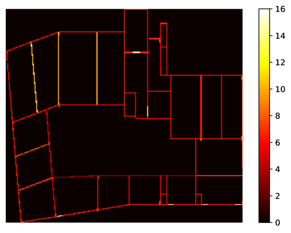
(a) Reflectance

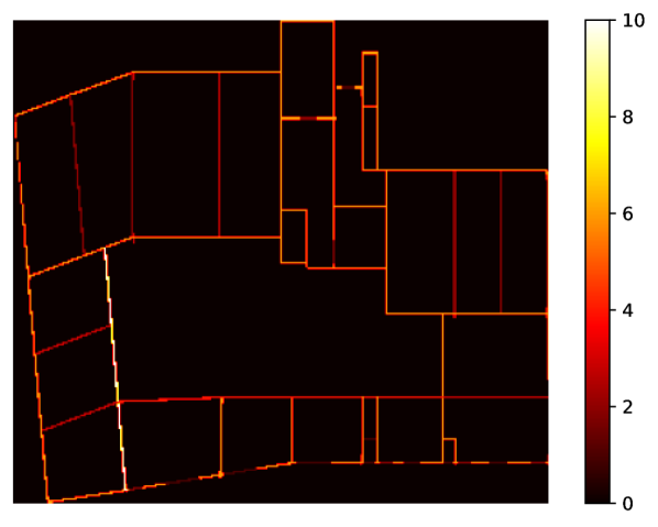
(b) Transmittance

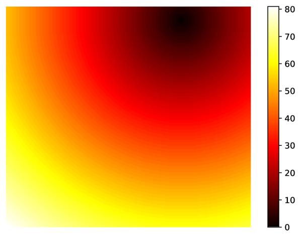
(c) Distance from antenna

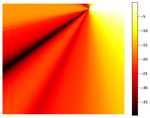
(d) Radiation pattern

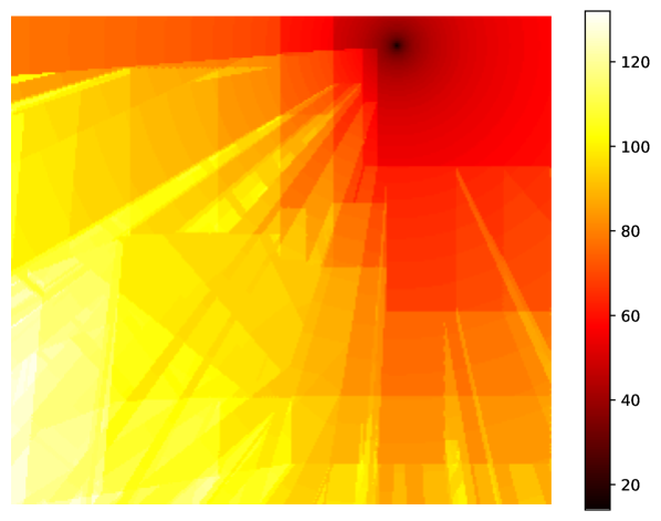
(e) Target

Figure 1: An example of the three given input channels (figs. 1(a), 1(b) and 1(c)), the radiation pattern channel that we created (fig. 1(d)), and the target (fig. 1(e)).

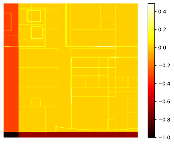
(a) Reflectance

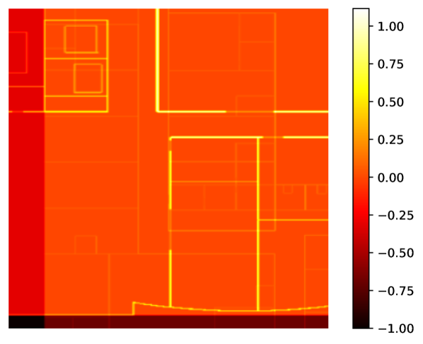
(b) Transmittance

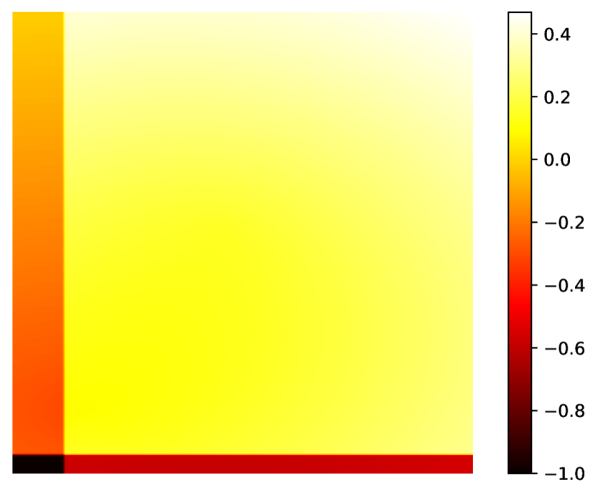
(c) Distance from antenna

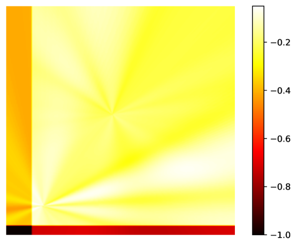
(d) Radiation pattern

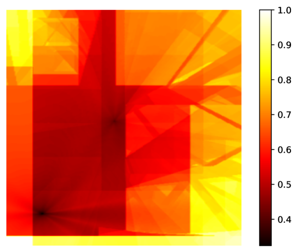
(e) Target

Figure 2: An example of the input (figs. 2(a), 2(b), 2(c) and 2(d)) channels, and the target (fig. 2(e)) for a training sample after applying all the augmentations, normalization and padding.

III Model Design and Neural Network Architecture

Our method is based on deep learning algorithms by utilizing minimal prior knowledge in the physics of radio signal propagation. We attempt to take a well-pretrained neural network and train it on the available training data by leveraging heavy data augmentation.

III-A Data Preprocessing

To ensure consistency, enhance feature representation, and improve the generalization capabilities of the model, a series of preprocessing steps were systematically applied to the dataset. These steps are designed to standardize the input data, address variations in geometry and dimensions, and facilitate the incorporation of additional context for specific tasks. The following techniques were employed:

III-A1 Data Preparation for Tasks 1, 2, and 3

To align with the specific requirements of Tasks 1, 2, and 3, we prepared the dataset as follows:

• Task 1: The input data consists of three channels—reflectance, transmittance, and distance. Each input image is padded to a square, and then resized to $518\times 518$. Padding is performed with values of $-1$, as $0$ holds meaningful significance in the dataset.

• Task 2: For the second and third tasks we need to include frequency information as well. Additionally, for task 3 we also need to incorporate the information about the antenna type. We chose to encode this information by introducing additional input channels of the same dimensionality.

• Task 3: To represent the antenna’s radiation pattern and simulate signal propagation in Task 3, we visualized signal strength as triangular regions radiating from the antenna’s location. The key steps are as follows:

  • Antenna Location Identification: The antenna’s position is determined by identifying the pixel with the minimum intensity in the third channel of the input image.

  • Signal Data and Azimuthal Adjustment: The radiation pattern data contains signal strength values for each 360 angles (0–359). An azimuth offset is applied to align the orientation of the antenna.

  • Triangular Signal Representation: For each angle, the following actions are taken:

    • Two angles, offset by $0.5^{\circ}$, are calculated to form the edges of the current triangle.

    • The triangle is defined by three points: the antenna’s location and two points determined by the angles and a maximum signal propagation length.

  • Signal Strength Encoding: Each triangle is filled with a signal strength value from the radiation pattern data, with pixel intensity representing the signal strength in the respective direction.

  The resulting radiation pattern visualizes the antenna’s signal coverage, providing spatial context for signal propagation and station placement, as illustrated in fig. 1(d).

III-A2 Normalization

We performed exploratory analysis on the provided data and determined the ranges of values for reflectance, transmittance and distance. We choose channel specific maximum values ($25$ for reflectance, $20$ for transmittance and $200$ for distance), divided each channel by those numbers. These normalized channels become an input for the models focused on the first task.

For encoding the frequency information, we simply create a channel with a constant value equal to the frequency in GHz, divided by 10 to ensure the values are less than $1$.

For normalizing the channel representing the radiation pattern, we also choose channel specific maximum values ($40$), and divided the channel by this number.

III-A3 Data Augmentation

Data augmentation is a critical step, especially when dealing with limited training data. By artificially increasing the diversity of the dataset, augmentation methods simulate various real-world scenarios and improve the generalization capability of the model. We applied the following augmentation techniques:

MixUp Augmentation

MixUp is an augmentation technique that generates data by blending pairs of input samples and their associated labels to create more generalized representations of the data. We employed this method to improve the model’s generalization and robustness. In our training pipeline, MixUp was applied to $75\%$ of the training data, while the remaining $25\%$ of the samples were left unaltered. This balanced approach ensures that the network is trained on both augmented and original data, enabling it to learn a diverse feature space while maintaining alignment with the original data distribution.

Rotation Augmentation

Rotation augmentation introduces variations in the orientation of input images, enhancing the model’s invariance to spatial transformations. During training, each input sample is randomly rotated by $0^{\circ}$, $90^{\circ}$, $180^{\circ}$, or $270^{\circ}$(multiples of $90^{\circ}$) degrees, chosen with equal probability. It is clear that in the case of $0^{\circ}$ no change occurs, which means that rotation is performed on approximately $75\%$ of the training data. This ensures that the network can distinguish between augmented and unaugmented orientations, learning more robust spatial features.

Cropping and Resizing

Cropping is employed to simulate partial observations of the input data. In this case, $75\%$ of the training data is also processed, leaving the rest unchanged. The side length of the square is chosen randomly from a range between half the size of the input image ($259$ pixels) and the full size ($518$ pixels). After cropping, the resulting square is resized back to $518\times 518$ to match the input dimensions required by the model.

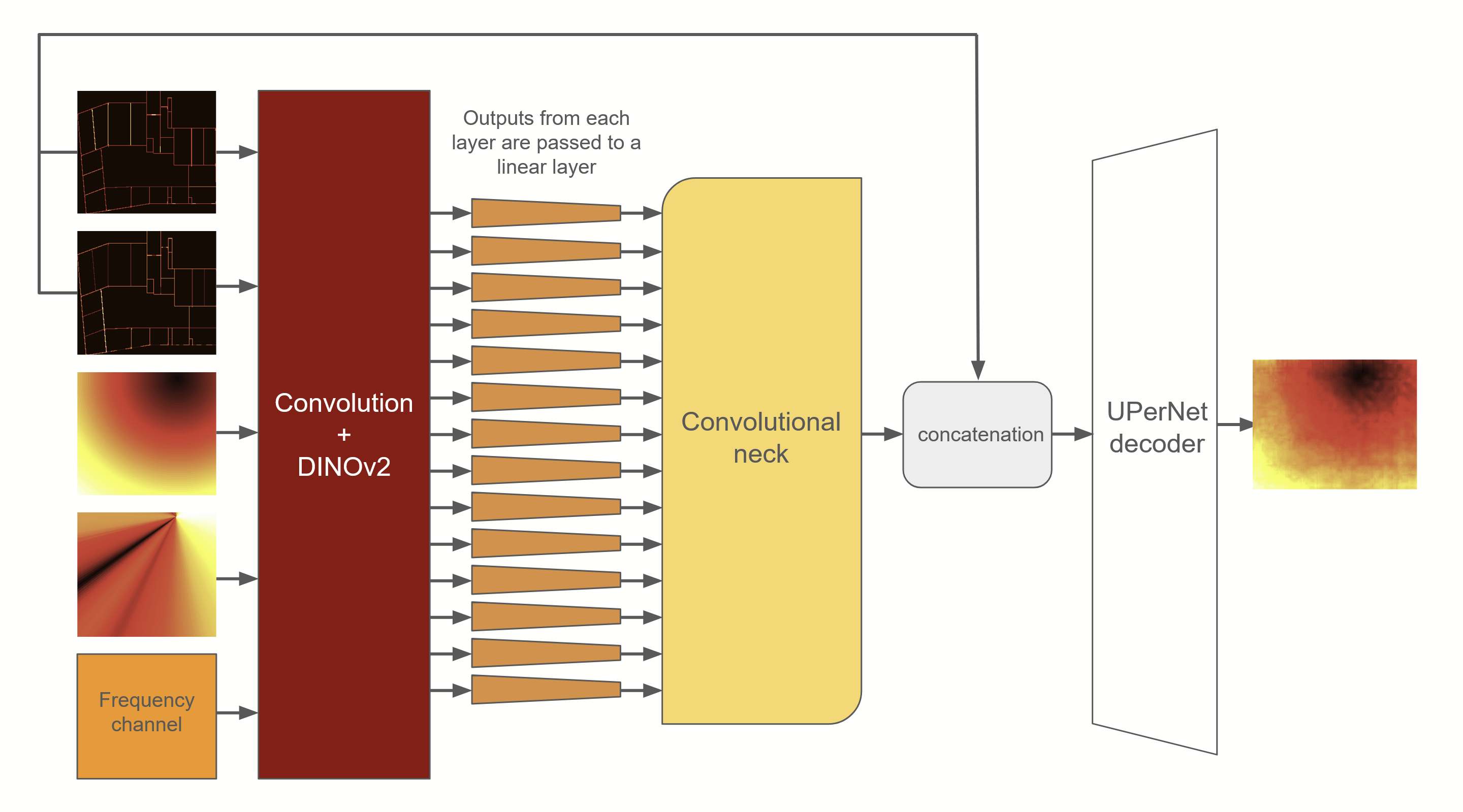
Figure 3: Model architecture

III-A4 Training, Validation, and Testing Splits

For our tasks, the dataset was partitioned into training, validation, and testing sets based on specific criteria. The splits for each task are detailed below:

• Dataset Structure:

  • Training data includes environments B1-19, with additional augmentations such as MixUp, rotation, and cropping.

  • Validation data includes environments B20-22, utilized without augmentation for task evaluation.

  • Testing data includes environments B23-25, preserved for final performance assessment.

• For Task 2:

  • Validation and Testing sets include frequency f2 for evaluation purposes.

• For Task 3:

  • Training data includes Ant1-3. Ant4 is saved for validation. And Ant5 is saved for testing to assess performance based on different antenna configurations.

So, for our validation and test, we are picking unseen rooms for Task 1, also unseen frequency for Task 2, and also unseen antenna for Task 3. The input channels and the target for a training example, after applying the preprocessing steps and augmentations, can be seen in fig. 2.

III-B Neural Network Design

Vision transformers (ViT) [9] have been prominently proven to achieve state-of-the-art results in image-based tasks and beyond. Moreover, we have a successful experience in adopting a ViT-based approach to map reconstruction based only on radio information [5]. In the previous section, we described the way the input data is represented as an image. In this section, we will present our proposed neural network based on the DINOv2 vision transformer.

Our neural network consists of three parts: DINOv2 vision transformer [10], used as an encoder, UPerNet convolutional decoder [11], and a neck responsible for connecting the Vit-based encoder and the convolutional decoder. We choose the ViT-B/14 version of DINOv2 with pre-trained weights. First, the input image is passed through a convolutional layer, which outputs a three-channel image. We do this for compatibility with the DINOv2 input, to be able to leverage the pre-trained weights of the network. The resulting image is passed to the encoder to obtain the embeddings of the image. Then the embeddings from all the 14 layers (the first layer, 12 hidden layers, and the output layer) are passed through a linear layer to decrease the embedding size from 768 to 256 for task 1, and 512 for tasks 2 and 3. The low-dimensional embeddings are then reshaped into 37*37 squares and fed to the neck, which consists of a convolutional layer with a ReLU activation function, a resize operation, and another convoultional layer with a ReLU activation function. The activations are then passed to the UPerNet decoder to obtain the output. To reinforce the room borders to the network, we also concatenate the reflectance and transmittance channels to the activations obtained from the neck, before feeding it to the decoder. Sigmoid function is then applied to the output, and the result is multiplied by 160 to get the final prediction.

The model architecture can be seen in fig. 3.

IV Results

Table I summarizes the performance across the three tasks. We report the performance on the test set, that we created and on the test set provided by the First Indoor Pathloss Radio Map Prediction Challenge at ICASSP 2025 [8]. These results secured the 8th place in the challenge.

Our analysis showed that the large difference between the scores on two test sets comes mostly from a distribution shift between building layouts. The layouts from the Challenge Test Set are significantly smaller and have denser walls. Development of methods to increase robustness of the deep learning models on such shifts is left for future work.

The results also show that our training strategy is quite robust with respect to changes in frequencies and antenna types. The degradation of performance between Task 1 and the other two tasks is less than 3.4 in absolute values, or 30% in relative terms, in the Challenge Test Set. This ratio is better than the degradation we have seen on our test set, and is comparable to the winner solutions of the Challenge. Whether this robustness comes from the input representation or the augmentation technique requires more ablation studies that is left for future work.

TABLE I: The RMSE (dBm) measured on our test set and the private test set for the three tasks.

Task	Our Test	Challenge Test	Winner Solution
Task 1	5.9	11.34	7.87
Task 2	9.1	14.75	10.10
Task 3	11.2	14.67	10.09
Weighted Average	8.98	13.695	9.427

References

- [1] Z. Xing and J. Chen, “Constructing indoor region-based radio map without location labels,” IEEE Transactions on Signal Processing, vol. 72, pp. 2512–2526, 2024.
- [2] R. Jaiswal, M. Elnourani, S. Deshmukh, and B. Beferull-Lozano, “Location-free indoor radio map estimation using transfer learning,” in 2023 IEEE 97th Vehicular Technology Conference (VTC2023-Spring), 2023, pp. 1–7.
- [3] H. Khachatrian, R. Mkrtchyan, and T. P. Raptis, “Deep learning with synthetic data for wireless nlos positioning with a single base station,” Ad Hoc Networks, vol. 167, p. 103696, 2025. [Online]. Available: https://www.sciencedirect.com/science/article/pii/S157087052400307X
- [4] R. Darbinyan, H. Khachatrian, R. Mkrtchyan, and T. P. Raptis, “Ml-based approaches for wireless nlos localization: Input representations and uncertainty estimation,” in 2023 IEEE Ninth International Conference on Big Data Computing Service and Applications (BigDataService), 2023, pp. 87–94.
- [5] H. Khachatrian, R. Mkrtchyan, and T. P. Raptis, “Outdoor environment reconstruction with deep learning on radio propagation paths,” in 2024 International Wireless Communications and Mobile Computing (IWCMC), 2024, pp. 1498–1503.
- [6] M. Becattini, D. Borsatti, A. Bujari, L. Carnevali, A. Garbugli, H. Khachatrian, T. P. Raptis, and D. Tarchi, “Empirical application insights on industrial data and service aspects of digital twin networks,” in 2024 IEEE International Mediterranean Conference on Communications and Networking (MeditCom), 2024, pp. 323–328.
- [7] X. Li, H. Li, H. K.-H. Chan, H. Lu, and C. S. Jensen, “Data imputation for sparse radio maps in indoor positioning,” in 2023 IEEE 39th International Conference on Data Engineering (ICDE), 2023, pp. 2235–2248.
- [8] S. Bakirtzis, C. Yapar, K. Qui, I. Wassell, and J. Zhang, “The first indoor pathloss radio map prediction challenge,” in To appear in Proc. IEEE International Conference on Acoustics, Speech, and Signal Processing Workshops (ICASSPW), April 2025.
- [9] A. Dosovitskiy, “An image is worth 16x16 words: Transformers for image recognition at scale,” arXiv preprint arXiv:2010.11929, 2020.
- [10] M. Oquab, T. Darcet, T. Moutakanni, H. Vo, M. Szafraniec, V. Khalidov, P. Fernandez, D. Haziza, F. Massa, A. El-Nouby et al., “Dinov2: Learning robust visual features without supervision,” arXiv preprint arXiv:2304.07193, 2023.
- [11] T. Xiao, Y. Liu, B. Zhou, Y. Jiang, and J. Sun, “Unified perceptual parsing for scene understanding,” in Proceedings of the European conference on computer vision (ECCV), 2018, pp. 418–434.