High Precision Binding Energies from Physics Informed Machine Learning

Abstract

Twelve physics informed machine learning models have been trained to model binding energy residuals. Our approach begins with determining the difference between measured experimental binding energies and three different mass models. Then four machine learning approaches are used to train on each energy difference. The most successful ML technique both in interpolation and extrapolation is the least squares boosted ensemble of trees. The best model resulting from that technique utilizes eight physical features to model the difference between experimental atomic binding energy values in AME 2012 and the Duflo Zucker mass model. This resulted in a model that fit the training data with a standard deviation of 17 keV and that has a standard deviation of 92 keV when compared all of the values in the AME 2020. The extrapolation capability of each model is discussed and the accuracy of predicting new mass measurements has also been tested.

I Introduction

Theoretical binding energies can provide guidance for experimental measurements facilities working on the frontiers of science (e.g., at CARIBU [1], at JYFLTRAP [2], and at FRIB [3, 4]). Further from stability, theoretical binding energies play a critical role in astrophysically relevant calculations for example regarding the r-process (e.g., Ref. [5], and [6]). The r-process occurs near the proton drip line where experimental measurements have not been thoroughly explored. For these cases and others high precision theoretical binding energies are sought out.

There has been a long history of binding energy models dating back to Refs. [7] and 8. The best contemporary atomic binding energies models typically reproduce Atomic Mass Evaluation (AME) experimental values for $N\geq 8$ and $Z\geq 8$, with standard deviations, denoted as $\sigma$, ranging from about 200-800 keV (for a summary discussion see Ref. [9] and the references therein, or Ref. [10]).

Recently, the use of Machine Learning (ML) techniques informed by a dozen or so physical features have been able to achieve models of binding energy using neural networks [11, 12], or Support Vector Machines (SVM) and Gaussian Process Regression (GPR), that also result in binding energy models in this range of accuracy [13]. A best fit value as low as $\sigma$=128 keV has been achieved using a kernel ridge regression which included odd-even effects [14]. The technique of training ML models informed by physical features has also been adapted to predict alpha decay [15], quadrupole deformations [16] and B(E2) values [17].

In this manuscript, we present a methodology, to predict the binding energy, involving four different ML approaches: SVM, GPR, neural networks, and ensemble of trees. In general SVM’s effectiveness is particularly evident when handling nonlinear regression challenges [18], often delivering superior outcomes to other techniques [19]. GPR is similarly kernel-based but it results in probabilistic models that are nonparametric [20, 21]. Artificial neural networks utilize hidden layers that mimic connections between neurons in the brain through activation functions and weights allowing them the ability to determine non-linear relations [22]. Ensemble of trees algorithms are widely utilized ML techniques for analyzing tabular data sets [23]. These ML approaches were used to train models on a subset of the AME 2012 data [24] based on groups of physical features.

Instead of modeling the binding energy directly, our approach consists of training ML models on the residual difference between the experimental values and one of three different mass models. The mass models used are two simple semi-empirical models and the Duflo Zucker [25] mass model. Section II discusses the binding energy models and data sets used to train and test. This alleviates the burden on the ML models of learning the underlying distribution of the binding energies and allows for the accomplishment of a potentially easier task of predicting just the difference in the binding energies. In essence, once the background of “theoretical prediction” is removed, it becomes easier to model the “signal” which is the difference between the experimental measurement and the theoretical predictions. In other words, what the ML model is left to learn from binding energy differences are the terms dependent of the physical features that are not explicitly accounted for in the theoretical models, i.e., higher-order effects in terms of the physical features. Furthermore, we explain the predictions of the models using Shapley values, a measure of feature importance derived from cooperative game theory.

Section III discusses the four ML approaches used and the relevant hyperparameters that have been optimized in each. Section IV discusses the process used to determine which physical features are critical to the ML model training. Section V discusses the process used to determine the best models and corresponding model fit metric values. This section also contains a discussion comparing the predictive power and extrapolation limitations of the different ML approaches.

II Determining the Training and Testing Data

When training ML models the preprocessing of the data is essential as it makes the learning task easier for the ML models. In this work, the preprocessing of the data comes in the form of removing one of three mass models from the experimental values.

II.1 Five Coefficient Model of Binding Energy

The process of creating a macroscopic mass model usually begins by treating the nucleus as a liquid drop of charged nuclear matter comprised of protons and neutrons. Modern versions of this technique can achieve models on the order of 400 keV [26].

In that spirit, a simple five-coefficient binding energy model was originally introduced as Eqn. (3) in Ref. [27] has been chosen, that is of the form:

$$\begin{split}B_{LD5}=&(a_{v}A+a_{s}A^{2/3})(1+\kappa T_{Z}(T_{Z}+1)A^{-2})+\\ &(a_{c}Z(Z-1)+\Delta)A^{-1/3})\end{split}$$ (1)

where the neutron number ($N$), proton number ($Z$), the mass number ($A$) and the isospin projection ($T_{Z}=(N-Z)/2$) are used. The pairing contribution used is $\Delta=+a_{p}$ if the nucleus is even-even, $\Delta=-a_{p}$ if odd-odd, and is $\Delta=0$ otherwise.

This expression contains the standard liquid droplet model surface and volume considerations. The $Z(Z-1)$ expansion results from the semi-classical treatment of the protons accounting for the interaction of each proton with all other protons. The expansion of the form $T_{Z}(T_{Z}+1)$ is consistent with experimental observations [28] and results from isovector pairing calculations in the strong pairing limit [29].

The coefficients $a_{v}=$15.79 MeV, $a_{s}=$-18.12 MeV, $\kappa=$-7.18, $a_{c}=$-0.7147 MeV, and $a_{p}=$5.49 MeV were chosen from the fit in Ref. [27] and when compared to the AME 2012 this results standard deviation of 2.662 MeV.

The difference between the experimental binding energy and the theoretical liquid drop binding energy:

$$\Delta B_{LD5}=B_{exp.}-B_{LD5},$$ (2)

will be the first of three residuals that ML models will be trained to match.

Figure 1: Binding energy difference, (a) $\Delta B_{LD5}$, (b) $\Delta B_{LD6}$, and (c) $\Delta B_{DZ}$, between the three theoretical models of interest experimental measurements from AME 2012 [24].

II.2 Six Coefficient Model of Binding Energy

The difference $\Delta B_{LD5}$ is demonstrated in Fig. 1a. In an attempt to model the remaining features which often peak at magic numbers of protons and neutrons, and peak even higher for doubly magic nuclei, the following variables have been used

$$\nu=\frac{2N-N_{max}-N_{min}}{N_{max}-N_{min}},$$ (3)

and

$$\zeta=\frac{2Z-Z_{max}-Z_{min}}{Z_{max}-Z_{min}},$$ (4)

where the minimum and maximum values are defined by the nearest magic numbers. This results in $\nu$ and $\zeta$ beginning with values that increase linearly from -1 when adding valence nucleons above a closed shell. It is 0 when mid-shell, and 1 when the next shell is closed as discussed in detail in Ref. [30]. In this analysis the magic numbers chosen are

$$N_{min/max}=[2,8,20,28,50,82,126,196],$$ (5)

and

$$Z_{min/max}=[2,8,20,28,50,82,114,124]$$ (6)

as motivated by gaps in Nilsson levels from Ref. [31].

To recreate the parabolas that peak for magic numbers of protons and neutrons demonstrated in Fig. 1a. The $\nu$ and $\zeta$ are added to create a sixth semi-empirical term that can be written as:

$$B_{LD6}=B_{LD5}+a_{Shell}(\nu^{2}+\zeta^{2})^{2}.$$ (7)

This function of $\nu$ and $\zeta$ peaks with a value of four for doubly magic nuclei, is one when there is one magic number, and the other nucleon is mid-shell, or is zero if both the protons and neutrons are mid-shell. The corresponding best fit has determined the new coefficient to be $a_{Shell}=2.77$ MeV.

The second residual $\Delta B_{LD6}$ is the difference:

$$\Delta B_{LD6}=B_{exp.}-B_{LD6}.$$ (8)

The inclusion of this $\nu$ and $\zeta$ based term has reduced the standard deviation between the model and the AME 2012 experimental values by approximately 1 MeV to 1.667 MeV. This has been included in Fig. 1b.

II.3 Duflo Zucker

For the final residual, we will utilize a well-known and trusted formula as opposed to attempting to further refine our own semi empirical models.

The Duflo Zuker (DZ) micro-macro mass formula has been chosen as the third option to calculate the binding energy residuals from. The DZ model using 28 parameters was published in 1995, and it had an accuracy of 375 keV for the 1751 nuclides with measured masses known at the time [25]. In the nearly 30 years since this model was introduced, it has been proven to provide an excellent binding energy estimate.

Again the residual used is the difference of the theoretical binding energy removed from the experimental binding energy:

$$\Delta B_{DZ}=B_{exp.}-B_{DZ}.$$ (9)

The resulting values have been displayed in Fig. 1c.

II.4 Nuclides used in the Training and Testing Sets

These three binding energy differences have been chosen to represent: 1) a crude model that does not consider shell structure, 2) another that does consider shell structure in a global manner, and 3) a more sophisticated and trusted model.

We find it critical to not train on the same data as is being tested. The training of all models discussed in this manuscript is based on the AME 2012 data [24]. The AME 2020 data [32] was used to create an independent testing set where none of the same nuclides were used.

The full AME 2012 contains experimental binding energy values for 2353 nuclides. In our procedure, some were removed and reserved for the training set. There are 17 nuclides that have experimentally measured values in AME 2012 but that are not found in the AME 2020. Those were removed from the training set. Additionally, 57 binding energy measurements changed by more than 100 keV when comparing AME 2020 with AME 2012. Those were also not included in the training set. Lastly, one out of every seven of the remaining nuclides (326 total) were also removed from the training set and were reserved for the test set. This last group were included so the test set can be representative of the entire set. In total 400 nuclei that are in the AME 2012 data set were not used to train.

In addition to the 57 nuclides with substantially changed binding energy values and the 326 corresponding to every seventh nuclide, there are 121 nuclides with new mass measurements in the AME 2020. Combined an independent set of 504 nuclides from AME 2020 were used to test the accuracy values from the models. Figure 2 demonstrates the testing set nuclides and the locations and reasoning for the testing set nuclides This represents approximately 20% of the total AME 2020 set.

Figure 2: The training set comprised of AME 2012 data along with the three constitutes of the testing set from AME 2020, specifically new values, changed values, and the selection for one out of every seven throughout.

Table 1 has been included to provide some perspective on how good each model is initially for the training, test, and full AME data sets. The number of nuclei and the mean Experimental Uncertainty ($\overline{EU}$) values have also been included for each data set. The value of $\overline{EU}=$20 keV is important because all models will be trained on a data set that has average uncertainties at this level.

Table 1: Data Set, Size, Mean Experimental Uncertainty, and Model Standard Deviation Comparison

Set	Train 2012	All 2012	Test 2020	All 2020
Number	1953	2353	504	2457
$\overline{EU}$	0.020 MeV	0.026 MeV	0.044 MeV	0.023 MeV
$\sigma_{\Delta B_{LD5}}$	2.638 MeV	2.662 MeV	2.773 MeV	2.666 MeV
$\sigma_{\Delta B_{LD6}}$	1.672 MeV	1.677 MeV	1.779 MeV	1.696 MeV
$\sigma_{\Delta B_{DZ}}$	0.384 MeV	0.393 MeV	0.561 MeV	0.427 MeV

III Machine Learning Approaches

Four ML approaches have been used to train models for each of the differences $\Delta B_{LD5}$, $\Delta B_{LD6}$, and $\Delta B_{DZ}$. To protect against overfitting, the training involved a five-fold cross-validation scheme, where the training data is partitioned and accuracy is estimated for each fold. The model hyperparameters were determined using a Bayesian optimization routine with the expected improvement per second plus acquisition function. The optimization process for each model was run for 250 iterations, though convergence often occurred within the first 50 iterations.

III.1 Support Vector Machines

We have implemented a variant of the SVM [33], the Support Vector Machine Regression (SVMR) [34], as one of our machine learning approaches. The success of an SVM based model in these scenarios hinges on the use of the kernel trick, a powerful technique for addressing data that is not linearly separable in its original feature space. By using the kernel trick, SVM implicitly transforms the data into a higher-dimensional space, where linear separability can be achieved [35]. This transformation is made possible through a kernel (covariance) function, which computes the dot product between data points in this higher-dimensional space without explicitly calculating the transformed features. As a result, SVM maps input data into a higher-dimensional space using kernel functions, enabling it to capture nonlinear relationships.

SVMR approach is specifically crafted for regression tasks, offering a distinctive method for predicting continuous values by applying the principles of SVMs. Unlike classification-based techniques, SVMR aims to identify a hyperplane that best models the training data while minimizing prediction errors. A key element of SVMR is its reliance on support vectors, which are the crucial data points located nearest to the hyperplane’s boundaries. The model strives to position as many data points as possible within this optimal hyperplane, adhering to a defined tolerance margin, while also managing instances where data points lie outside the boundary. This introduces a hyperparameter, which determines the hyperplane’s width.

Similar to Ref. [13], we have determined that the Gaussian kernel of the form:

$$K_{G}(x_{i},x_{j})=e^{-\gamma r^{2}}$$ (10)

generates the most reliable models. Here $x_{i}$, and $x_{j}$ represent two data points, and $r$ is the Euclidean distance between the two points:

$$r=||x_{i}-x_{j}||=\sqrt{(x_{i}-x_{j})^{T}(x_{i}-x_{j})}$$ (11)

and $\gamma$ is the kernel coefficient.

The optimized hyperparameters are the kernel scale, box constraint (labeled $C$) which controls the penalty imposed on observations with large residuals, and the $\epsilon$ values that govern the margin of tolerance.

III.2 Gaussian Process Regression

Gaussian Process Regression (GPR) works by using modeling a Gaussian distribution over possible functions. The algorithm begins by defining a prior distribution over these functions, where the function values at the input points follow a Gaussian distribution [21]. This prior is based on a mean function and a kernel function, which sets the initial assumptions.

As training data is introduced, the prior is updated to form a posterior distribution by applying Bayes’s theorem. This update integrates the observed data, adjusting the model’s understanding of the underlying function. The posterior distribution then allows for predictions at new data points, offering not just a predicted mean but also a measure of uncertainty, which is especially valuable for making decisions in uncertain environments.

The strength of GPR lies not only in its predictive accuracy but also in its capacity to provide detailed insights into the confidence of those predictions. This is accomplished through its uncertainty quantification, which offers a probabilistic assessment of how reliable each prediction is. By accurately measuring the uncertainty associated with each outcome, GPR significantly improves decision-making processes. This combination of delivering accurate predictions while simultaneously evaluating their reliability makes GPR a powerful tool.

We have trained our GPR models using the Isotropic Matern 5/2 kernel function which also involves $r$ from Eqn. (11) which of the form:

$$K_{M5/2}(x_{j},x_{k})=\sigma_{f}^{2}(1+\sqrt{5}r/\sigma_{l}+5r^{2}/{3\sigma_{l}^{2}})e^{-\sqrt{5}r/\sigma_{l}}$$ (12)

where $\sigma_{l}$ is the characteristic length scale and $\sigma_{f}$ is the signal noise standard deviation.

The optimized hyperparameters in this approach are the kernel scale, the type of the basis function used either zero, constant, or linear, and $\sigma_{f}$.

III.3 Neural Networks

Neural Networks are differentiable universal function approximators that have non-linearity introduced through activation functions that act on a affine transformation of the input using learnable weights and biases [36, 37]. Implemented as multi-layer perceptrons, they are nested functions represented by hidden layers that are fully connected. The complexity or expressivity of a neural network relies on the number of hidden layers representing the depth of nesting and the width of the hidden layers representing the number of activations summed over in each layer.

Our approach involves Fully Connected Neural Network (FCNN) models with one, two, or three hidden layers. The options tested for the number of nodes on each hidden layer were: [300], [1000], [10 10], [100 100], [200 200], [300 300] [10 10 10], [100 100 100], [200 200 200], [300 300 300], [400 400 400]. Additionally, three activation functions were tested ReLU, sigmoid, and tanh. An $L2$ regularization was used requiring the optimization of a hyperparameter corresponding to the regularization strength (denoted as $\lambda$).

III.4 Ensemble of Trees

Ensemble of trees based algorithms utilize multiple base decision trees, each trained on a separate subset of the data. Notable examples of tree-ensemble algorithms include Random Forests [23], Gradient Boosted Decision Trees [38]), or the Least Squares Boosting (LSBET) [39].

Among these ensemble algorithms, we have determined that LSBET is the preferred technique for modeling binding energy residuals. It effectively leverages the strengths of boosting and decision trees to improve predictive accuracy in regression scenarios. The process begins by initializing the first trees, then predicting the residuals, and then based on the prediction a step is taken which is scaled by the learning rate (denoted as $\eta$). Finally. the squared error between the predicted and true values is minimized. Overfitting can be protected against by using a low learning rate, regulating the maximum depth of the trees and limiting the number of boosting rounds.

In our tests, we varied the number of learners to be 10, 100, 300, 1000, 1500, 3000, 6000, 9000, and 12000 for these calculations and the optimized hyperparameters are the minimum leaf size and the learning rate.

IV Physical Feature Selection

Our approach is to determine binding energies based on ML approaches that have been trained on energy residuals coming from each of the $\Delta B$ sets. This differs from the prior works, specifically Refs. [11] and [13] where the binding energy values are used directly. Training ML models on the residuals may lead to more accurate models and it may reduce the number of physical features used.

Two pairs of quantities directly related to the number of particles in the nucleus have been included in the groups $N$, $Z$, $T_{Z}$, and $A$.

The two linear shell structure parameters from the added term in $B_{LD6}$, namely, $\nu$ and $\zeta$ have also been added. This is similar to the inclusion of the valence neutron ($V_{N}=N-N_{min}$) and valence proton ($V_{Z}=Z-Z_{min}$) numbers using Eqns. (5) and (6), and Casten’s P factor from Ref. [40] (where $P=(V_{N}V_{Z})/(V_{N}+V_{Z})$) used in other works.

The spherical sub-shell number for the last occupied neutron and proton, denoted as $N_{S}$, and $Z_{S}$, respectively has also been included. This is similar to the use of shell terms in Refs. [11] and [13], but in this case, the sub-shell count was used as opposed to the major shell.

If, for example, $N=9-14$, then according to the spherical Nilsson model (from the Nuclear Structure section of Ref. [31]) the valence neutron will be on $1p_{3/2}$, by the counting up from zero $N_{S}=4$. If $N=15-16$, then $1p_{1/2}$ will be occupied and $N_{S}=5$. If $N=17-20$, then $1d_{5/2}$ will be occupied and $N_{S}=6$, and so on. Using the sub-shell as opposed to the major shell number provides the ML models more flexibility to train on a wider variety of features. If the major shell is an important feature then for example $N_{S}=4,5,$ and $6$ can be treated identically and effectively grouped within the model corresponding so that it behaves as one large oscillator shell.

The fifth group of parameters included to provide modifications resulting from even-odd mass staggering. These are Boolean values accounting for whether the number of nucleons is even or odd. These are written as $N_{E}$, and $Z_{E}$ and the value is 1 if the respective neutron or proton number is even, or 0 if it is odd.

The five pairs of features that could be combined as $2^{5}-1=31$ possible groups. A preliminary set of calculations was made for each ML approach on each $\Delta B$ value where all 10 physical features were included. A subsequent analysis of those preliminary calculations using Shapley values allowed for restrictions on the number of groups to be determined. Shapley values [41] provide a means of determining the contribution of different players in a cooperative game. Here they were used to determine the contribution of each input variable for predicting the output variable in each ML model.

The Shapley value analysis indicated that in some cases, only six or eight features are necessary. The six features with the highest dependence consist of $N,Z,T_{Z}$, and $A$ as well as one pair of shell-related features, either $\nu$ and $\zeta$, or $N_{S}$ and $Z_{S}$, depending on the ML approach. Regarding the top eight, the least influential features were often $N_{E}$ and $Z_{E}$, but there were also cases where the weakest dependence was from either pair of shell features.

A feature group containing only $N$ and $Z$ has also been included to serve as a baseline. In total seven groups of features implemented in the following analysis are shown in Tab. 2.

Table 2: Physical Features Used with ML Models

Feature	Number of	Physical
Group	Features	Features
1	2	$N,Z$
2	6	$N,Z,T_{Z},A,\nu,\zeta$
3	6	$N,Z,T_{Z},A,N_{S},Z_{S}$
4	8	$N,Z,T_{Z},A,\nu,\zeta,N_{S},Z_{S}$
5	8	$N,Z,T_{Z},A,\nu,\zeta,N_{E},Z_{E}$
6	8	$N,Z,T_{Z},A,N_{S},Z_{S},N_{E},Z_{E}$
7	10	$N,Z,T_{Z},A,\nu,\zeta,N_{S},Z_{S},N_{E},Z_{E}$

V Results and Discussion

In the following subsections, the methodology used to determine the best models will be discussed. In the interest of clarity in describing how well the ML models perform, we will try to share the comparison metrics for multiple data sets including the training set, the independent testing set, as well as the entire AME 2012 and AME 2020 data sets.

V.1 Determining the Best Model

The best model was determined for each of the three residuals using each of the ML approaches. Although the standard deviation is often the metric discussed concerning binding energy model accuracy. The standard deviations by construction emphasize the furthest outliers. When comparing nuclei from $N\geq 8$ and $Z\geq 8$ the largest deviations are often among the data for the lower mass nuclei. Instead of determining the best model based on the standard deviation an alternative metric has been chosen.

The twelve models were determined using the smallest value the mean Absolute Error ($\overline{AE}$) for the independent testing data set of AME 2020 data. The $\overline{AE}$ values are preferable because they represent the mean absolute deviation between the model and the experimental values. So the use of $\overline{AE}$ will help mitigate a low mass bias.

Figure 3a demonstrates why the best LD6BET model was determined to be Feature Group 3. In this case, the model with only 6 physical features outperformed models with 8 or 10. This is of interest because prior to this the literature primarily demonstrates the best model having the most features.

Figure 3: The mean absolute error for $\Delta B_{LD6}$ LSBET calculations (a) as a function of the Feature Group for 3000 learners and (b) as a number of learners for Feature Group 3.

In general, determining the best models for SVMR, GPR, and FCNN was straightforward. The $\overline{AE}$ values for all models for all feature groups were sorted and the lowest value determined the best model. For FCNN, the largest models (in both the number of layers and the number of nodes on those layers) were not found to provide the best results.

In the case of the LS6BET, improvement of the test set $\overline{AE}$ values did continue with the increase in model size, but the improvement was marginal. In Figure 3b the number model performance for Feature Group 3 was plotted against the number of learners. The $\overline{AE}$ of the test set with 1000 learners was 4% above the minimum, with 1500 learners it was 1% above, and for 3000 learners it was 0.09% above the best possible model with 12000 learners. In all three $\Delta B$ sets a cap of 3000 was imposed and the results were less than 1% above of the best values calculated.

Table 3 contains the model, the feature group with the lowest $\overline{AE}$ value for the test set as as well as the comparison metrics for the training set, the entire AME 2012, and the AME 2020 set. In this table, multiple models have $\sigma$ and $\overline{AE}$ less than 100 keV depending on the data set compared.

Table 3: Best trained models and corresponding evaluation metrics for $\Delta B_{LD5}$, $\Delta B_{LD6}$, and $\Delta B_{DZ}$ using both AME 2012 [24], and AME 2020 [32] data.

Model	Feature	$\sigma_{12Train}$	$\overline{AE}_{12Train}$	$\sigma_{12}$	$\overline{AE}_{12}$	$\sigma_{20Test}$	$\overline{AE}_{20Test}$	$\sigma_{20}$	$\overline{AE}_{20}$
Name	Group	(MeV)	(MeV)	(MeV)	(MeV)	(MeV)	(MeV)	(MeV)	(MeV)
LD5SVMR	7	0.097	0.048	0.150	0.067	0.352	0.191	0.182	0.077
LD5GPR	7	0.067	0.037	0.124	0.055	0.321	0.171	0.158	0.065
LD5FCNN	7	0.070	0.052	0.145	0.074	0.395	0.195	0.190	0.082
LD5LSBET	6	0.018	0.014	0.117	0.043	0.317	0.208	0.145	0.055
LD6SVMR	5	0.111	0.049	0.171	0.071	0.385	0.196	0.201	0.080
LD6GPR	5	0.054	0.028	0.121	0.048	0.350	0.170	0.166	0.058
LD6FCNN	7	0.135	0.100	0.192	0.120	0.436	0.237	0.231	0.128
LD6LSBET	3	0.018	0.013	0.114	0.041	0.328	0.193	0.150	0.051
DZSVMR	7	0.073	0.051	0.111	0.066	0.277	0.168	0.142	0.074
DZGPR	6	0.066	0.046	0.103	0.062	0.226	0.150	0.118	0.067
DZFCNN	7	0.119	0.090	0.151	0.104	0.303	0.199	0.173	0.112
DZLSBET	6	0.017	0.013	0.084	0.034	0.199	0.130	0.092	0.039

Of the 12 best, the GPR and the LSBET-based models often outperform those from the SVMR and FCNN models. The best of the best is the DZLSBET model. It was fit to the training data with both $\sigma$ and $\overline{AE}$ values below 20 keV, while this low value should send a concern about overfitting. It performed the best against the test set with both metrics below 200 keV. The overall performance of this model compared to both the AME 2012 and AME 2020 are below 100 keV for all metrics.

V.2 Understanding the Models

One important feature of binding energy models is their ability to extrapolate. Figure 4 shows the resulting models for the 12 best. The first row of this figure contains the SVM models. Our results demonstrate that the SVM will have limited reach in extrapolation. There are noticeable features near where the data was trained but further away the value defaults to a constant value. The impact this has is that the model will predict something new for about a dozen more nuclei after the last known along an isotopic chain, but by two dozen the model will be contributing little to nothing.

The GPR-based models similarly can have the behavior of defaulting to a constant value far from stability. In the LD5GPR and LD6GPR models, this was off the scale of the calculations, but in the DZGPR model, the occurrence was similar to the observation in the SVM models. This will be demonstrated more clearly in Section V.4.

The LD5FCNN and LD6FCNN models are still good models for interpolated values though they aren’t as accurate as the others, and the extrapolation demonstrated in Fig. 4 is off scale for regions of potential astrophysical interest. The LSBET model curves on the other hand demonstrate that these models continue to predict new structures far from stability but it is on scale with the trained values.

Figure 4: The 12 Best $\Delta B$ models. (a) LD5SVM with $C=113$ and $\epsilon=0.046$, (b) LD6SVM with $C=382$ and $\epsilon=0.040$, (c) DZSVM with $C=82.1$ and $\epsilon=0.049$, (d) LD5GPR with linear basis function and $\sigma_{f}=0.00148$, (e) LD6GPR with zero basis function and $\sigma_{f}=0.0496$, (f) DZGPR with zero basis function and $\sigma_{f}=0.0456$, (g) LD5FCNN with a tanh activation function, two layers each consisting of 200 nodes, and $\lambda=5.73\times 10^{-5}$, (h) LD6FCNN with a sigmoid activation function, two layers each consisting of 100 nodes, and $\lambda=1.39\times 10^{-4}$, (i) DZFCNN with a tanh activation function, two layers each consisting of 100 nodes, and $\lambda=4.98\times 10^{-4}$, (j) LD5LSBET with 3000 learners, a minimum leaf size of 2, and $\eta=0.102$, (k) LD6LSBETwith 3000 learners, a minimum leaf size of 2, and $\eta=0.131$, (l) DZLSBET with 3000 learners, a minimum leaf size of 1, and $\eta=0.0819$.

Figure 5 shows the Shapley value results for all 12 models. These swarm charts show the distribution of Shapley values that are indicative of the importance of each physical feature in making predictions for each model. The vertical ordering of the physical features has been sorted in the order of importance in the model from high to low.

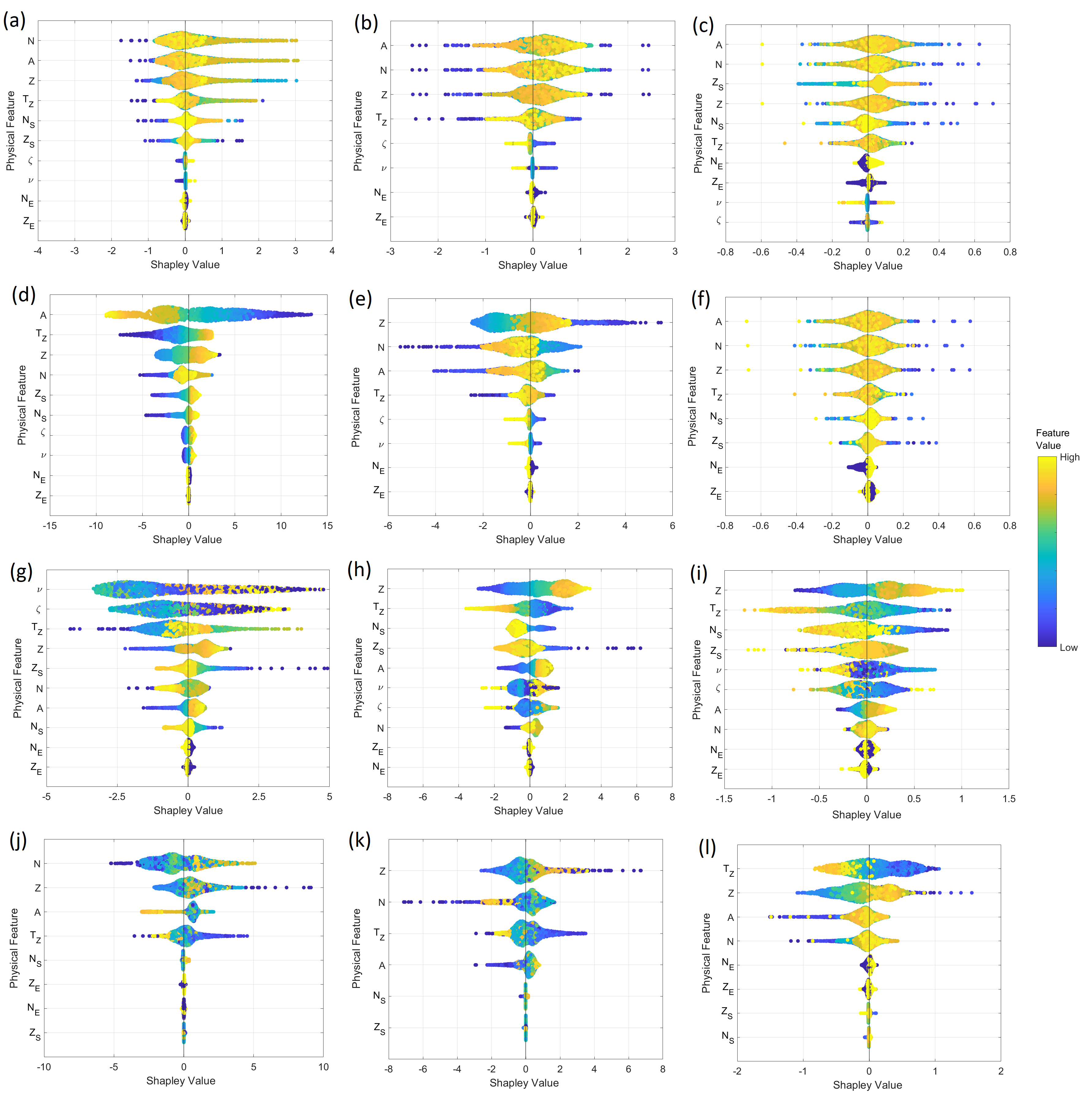
Figure 5: Distribution of local Shapley values for the 12 best models listed in order of feature importance for (a) LD5SVM, (b) LD6SVM, (c) DZSVM, (d) LD5GPR, (e) LD6GPR, (f) DZGPR, (g) LD5FCNN, (h) LD6FCNN, (i) DZFCNN, (j) LD5LSBET, (k) LD6LSBET, and (l) DZLSBET. The vertical spread in points represents how many values are located in the same region. The predictor value color demonstrates if the value for the given input predictor was high or low. Please note that the shapley value scale varies among the subplots.

In all of the SVM models and the DZGPR model, the Shapley values are generally low and independent of the value of the physical feature input. This corresponds to models with complex nonlinear behavior. On the other hand, the Shapley values have a broader distribution for the LSBET models in general and for the LD5GPR. This signifies that larger variance in the prediction can be achieved with these models which, in turn, explains the better performance of these models on the test sets. In particular, DZLSBET, which outperforms all other models, shows a clear hierarchy of the physical variables and also a broad spread of the Shapley values for the top four physical features. Therefore, the DZLSBET can effectively model $\Delta B_{DZ}$. From the lower right panel, it can be seen that $T_{Z}$, $Z$, $A$, and $N$ are the most important physical features in predicting $\Delta B_{DZ}$ with $N_{E}$, $Z_{E}$, $Z_{S}$, $N_{S}$ being not important in making these predictions. This shows that, in principle, even just a four parameter model might be sufficient.

V.3 Comparing with New Mass Excess Measurements

Table 4: Mass excess values from new measurements and differences ($\Delta ME=ME_{Exp.}-ME_{Model}$). All values in keV.

Isotope	$ME_{Exp.}$	$\Delta ME$	$\Delta ME$	$\Delta ME$	$\Delta ME$	$\Delta ME$	$\Delta ME$	$\Delta ME$	$\Delta ME$	$\Delta ME$	$\Delta ME$
& Ref.	(error)	DZ	HFB31	FRDM2012	WS4	LD5GPR	LD5LSBET	LD6GPR	LD6LSBET	DZGPR	DZLSBET
56V [42]	-46268(14)	-478	162	-1188	300	-156	-156	-184	-162	-181	-152
57V [42]	-44371(15)	-211	879	-592	652	16	104	-500	52	4	-37
58V [42]	-40361(44)	-51	559	-393	322	110	249	-451	47	40	106
95Ag [43]	-59743.3(14)	-273	-503	322	415	295	-226	111	-233	317	45
96Ag [43]	-64656.69(95)	-786	423	137	-146	-94	-151	-159	-155	-180	-136
104Y [44]	-53995(16)	-295	-485	609	-334	-283	-267	-317	-321	-510	-314
106Zr [44]	-58582.7(43)	948	-93	1311	-162	22	123	133	158	391	81
109Nb [44]	-56810(180)	870	190	983	-471	-205	-197	-201	-191	-122	-193
112Mo [44]	-57449(118)	1101	341	962	85	-172	19	-172	314	-212	139
119Cd [45]	-84064.8(21)	206	-135	-369	522	-30	-75	-55	-75	-54	-68
103Sn [46]	-67138(68)	212	-248	1023	83	58	-686	95	102	148	-73
	$\sigma$	622	437	806	362	165	250	215	192	256	140

New mass measurements continue to be made, which can serve as a second independent test set for our models. Table 4 contains Mass Excess values from five manuscripts [42, 43, 44, 45, 46] describing experimental measurements that have occurred since AME 2020 [32]. All the comparisons in the listed references where the measurement was either new or differed by more than 60 keV from AME 2020 have been included in Tab. 4.

For the sake of brevity, only the mass excess values resulting from GPR and LSBET models have been included. For comparison, the difference in mass excess between the new experimental measurement following models have also been provided: Duflo Zuker (DZ) [25], Hartree Fock Bogoliubov (HFB31) [10], Finite Range Liquid Droplet (FRDM12) [47], and Weizsäcker–Skyrme (WS4) [48]. Each of these six new models outperforms the contemporary mass models. The standard deviation of the 11 new measurements compared to each model has been included at the bottom of the table.

V.4 Comparing Extrapolations

Again for the sake of brevity, the extrapolation capability discussion will focus on the six GPR and LSBET models. The extrapolation behavior of the models can be seen in Figure 6. There is a spread among the GPR and LSBET models but in every case that spread is considerably less than that seen in the four mass models included in the comparison.

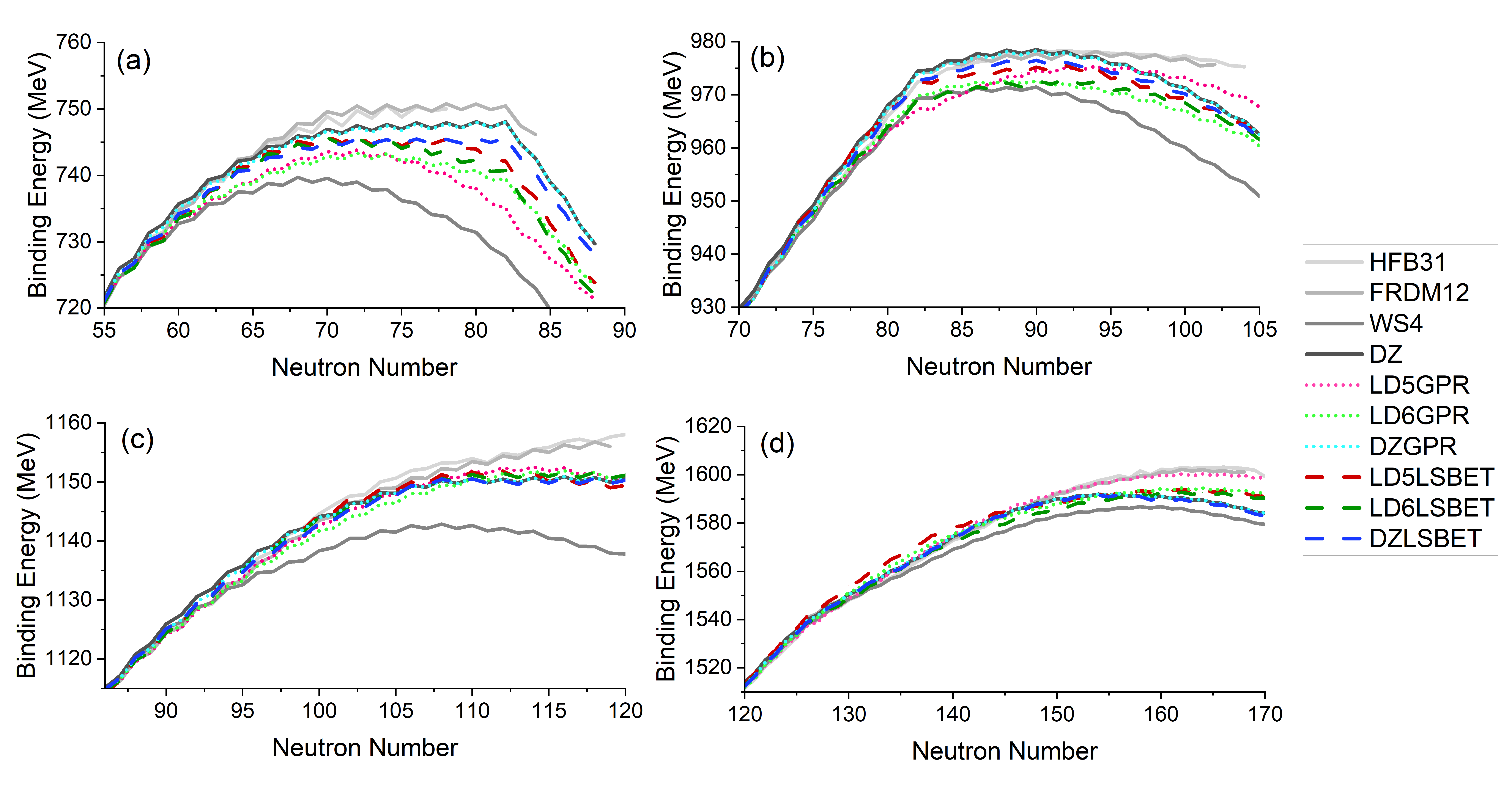
Figure 6: Mass model extrapolation comparison for neutron-rich (a) germanium, (b) molybdneum, (c) tin, and (d) tungsten isotopes. Dotted lines denote GPR models and dashed lines indicate LSBET models Four mass models, from Ref. [25], [10], [47], and [48], have been included in gray solid lines to allow for comparison.

In Figure 6c, the tin isotopes demonstrate consistent results for the six ML models which happen to also coincide with the DZ model.

In every subfigure, the DZGPR model converges to become indistinguishable from DZ toward the end of the extrapolation. For this reason, the preferred approach described here is the LSBET. It is interesting that the spread in extrapolation from among the three different LSBET models

VI Summary and Conclusion

In this work, we have created a methodology for producing accurate and predictive ML models that can improve binding energy models. Four ML approaches (SVMR, GPR, FCNN, and LSBET) were used to model binding energy residuals that resulted from comparing three different mass models ($\Delta B_{LD5}$, $\Delta B_{LS6}$, $\Delta B_{DZ}$) from an AME 2012 based training set. The different ML models were trained on groups of up to 10 physical features. Here it is worth noting that nearly all of the physical features are related to the number of protons and/or neutrons in some manner.

To protect against overfitting the metric used to evaluate model performance was the $\overline{AE}$ values determined for an independent set of 504 nuclei from the AME 2020. The $\overline{AE}$ values were preferred over the $\sigma$ values because they treat every comparison equally, whereas the $\sigma$ values can focus on outliers and a few dozen outliers can skew the results.

In some cases, better performance was achieved with fewer physical features. In total half of the best models contained 10 physical features while the other half used fewer than 10 physical features.

SVMR and GPR are techniques that are capable of providing good interpolations of data, but their ability to extrapolate is limited and they stop contributing when taken too far from range of the training data. FCNN and LSBET both continue to predict features far from stability based on the features learned elsewhere. FCNN and LSBET can be designed with variable size but it is worth noting that although the accuracy of the trained models generally continues to improve with more nodes or more learners, the independent test set demonstrated convergence and the best models required fewer nodes and fewer learners than the maximum numbers tested. Further, the best FCNN models all contained two hidden layers, outperforming larger networks with three layers.

Overall, the best ML models were consistently produced by GPR and LSBET. These approaches were used to generate models that resulted in $\sigma$ values of the full AME 2020 for the $\Delta B_{LD5}$ and $\Delta B_{LD6}$ that were the order of $150keV$. The best model produced overall which was based on $\Delta B_{Dz}$ results in a $\sigma$ value of $92keV$ and $\overline{AE}=39keV$ for the full AME 2020 data set. This was confirmed by explaining the models with Shapley values.

The results from the LSBET models strike a balance of predicting new features far from stability while remaining generally on the scale with the values seen experimentally near stability. This coupled with their strong performance regarding the fit metrics indicates that their use should be explored further potentially to create other models of nulcear properites.

References

- Hirsh et al. [2016] T. Y. Hirsh, N. Paul, M. Burkey, A. Aprahamian, F. Buchinger, S. Caldwell, J. A. Clark, A. F. Levand, L. L. Ying, S. T. Marley, G. E. Morgan, A. Nystrom, R. Orford, A. P. Galván, J. Rohrer, G. Savard, K. S. Sharma, and K. Siegl, First operation and mass separation with the caribu mr-tof, Nuclear Instruments and Methods in Physics Research Section B: Beam Interactions with Materials and Atoms 376, 229 (2016), proceedings of the XVIIth International Conference on Electromagnetic Isotope Separators and Related Topics (EMIS2015), Grand Rapids, MI, U.S.A., 11-15 May 2015.
- Vilen et al. [2018] M. Vilen, J. M. Kelly, A. Kankainen, M. Brodeur, A. Aprahamian, L. Canete, T. Eronen, A. Jokinen, T. Kuta, I. D. Moore, M. R. Mumpower, D. A. Nesterenko, H. Penttilä, I. Pohjalainen, W. S. Porter, S. Rinta-Antila, R. Surman, A. Voss, and J. Äystö, Precision mass measurements on neutron-rich rare-earth isotopes at jyfltrap: Reduced neutron pairing and implications for -process calculations, Phys. Rev. Lett. 120, 262701 (2018).
- Thoennessen [2024] M. Thoennessen, 2023 update of the discoveries of nuclides, International Journal of Modern Physics E 33, 2430001 (2024), https://doi.org/10.1142/S0218301324300017 .
- Wei et al. [2024] J. Wei, C. Alleman, H. Ao, B. Arend, D. Barofsky, S. Beher, G. Bollen, N. Bultman, F. Casagrande, W. Chang, Y. Choi, S. Cogan, P. Cole, C. Compton, M. Cortesi, J. Curtin, K. Davidson, S. D. Carlo, X. Du, K. Elliott, B. Ewert, A. Facco, A. Fila, K. Fukushima, V. Ganni, A. Ganshyn, T. Ginter, T. Glasmacher, A. Gonzalez, Y. Hao, W. Hartung, N. Hasan, M. Hausmann, K. Holland, H. Hseuh, M. Ikegami, D. Jager, S. Jones, N. Joseph, T. Kanemura, S. Kim, C. Knowles, T. Konomi, B. Kortum, N. Kulkarni, E. Kwan, T. Lange, M. Larmann, T. Larter, K. Laturkar, M. LaVere, R. Laxdal, J. LeTourneau, Z.-Y. Li, S. Lidia, G. Machicoane, C. Magsig, P. Manwiller, F. Marti, T. Maruta, E. Metzgar, S. Miller, Y. Momozaki, M. Mugerian, D. Morris, I. Nesterenko, C. Nguyen, P. Ostroumov, M. Patil, A. Plastun, L. Popielarski, M. Portillo, A. Powers, J. Priller, X. Rao, M. Reaume, S. Rodriguez, S. Rogers, K. Saito, B. Sherrill, M. Smith, J. Song, M. Steiner, A. Stolz, O. Tarasov, B. Tousignant, R. Walker, X. Wang, J. Wenstrom, G. West, K. Witgen, M. Wright, T. Xu, Y. Yamazaki, T. Zhang, Q. Zhao, S. Zhao, P. Hurh, S. Prestemon, and T. Shen, Technological developments and accelerator improvements for the frib beam power ramp-up, Journal of Instrumentation 19 (05), T05011.
- Mumpower et al. [2016] M. Mumpower, R. Surman, G. McLaughlin, and A. Aprahamian, The impact of individual nuclear properties on r-process nucleosynthesis, Progress in Particle and Nuclear Physics 86, 86 (2016).
- Brett et al. [2012] S. Brett, I. Bentley, N. Paul, R. Surman, and A. Aprahamian, Sensitivity of the r-process to nuclear masses, The European Physical Journal A 48, 184 (2012).
- Weizsäcker [1935] C. F. v. Weizsäcker, Zur theorie der kernmassen, Zeitschrift für Physik 96, 431 (1935).
- Myers and Swiatecki [1966] W. D. Myers and W. J. Swiatecki, Nuclear masses and deformations, Nuclear Physics 81, 1 (1966).
- Sobiczewski et al. [2018] A. Sobiczewski, Y. Litvinov, and M. Palczewski, Detailed illustration of the accuracy of currently used nuclear-mass models, Atomic Data and Nuclear Data Tables 119, 1 (2018).
- Goriely et al. [2016] S. Goriely, N. Chamel, and J. M. Pearson, Further explorations of skyrme-hartree-fock-bogoliubov mass formulas. xvi. inclusion of self-energy effects in pairing, Phys. Rev. C 93, 034337 (2016).
- Lovell et al. [2022] A. E. Lovell, A. T. Mohan, T. M. Sprouse, and M. R. Mumpower, Nuclear masses learned from a probabilistic neural network, Phys. Rev. C 106, 014305 (2022).
- Zeng et al. [2024] L.-X. Zeng, Y.-Y. Yin, X.-X. Dong, and L.-S. Geng, Nuclear binding energies in artificial neural networks, Phys. Rev. C 109, 034318 (2024).
- Yüksel et al. [2024] E. Yüksel, D. Soydaner, and H. Bahtiyar, Nuclear mass predictions using machine learning models, Phys. Rev. C 109, 064322 (2024).
- Wu et al. [2021] X. Wu, L. Guo, and P. Zhao, Nuclear masses in extended kernel ridge regression with odd-even effects, Physics Letters B 819, 136387 (2021).
- Li et al. [2022] C.-Q. Li, C.-N. Tong, H.-J. Du, and L.-G. Pang, Deep learning approach to nuclear masses and -decay half-lives, Physical review. C 105 (2022).
- Lin et al. [2024] Y. Lin, J.-X. Li, and H.-F. Zhang, Transfer learning and neural networks in predicting quadrupole deformation*, Chinese Physics C 48, 064106 (2024).
- Lv et al. [2024] B. Lv, Z. Li, Y. Wang, and C. Petrache, Mapping low-lying states and b(e2;01+→21+) in even-even nuclei with machine learning, Physics Letters B 857, 139013 (2024).
- Vapnik [2000] V. N. Vapnik, The Nature of Statistical Learning Theory (Springer New York, NY, 2000).
- Schölkopf and Smola [2001] B. Schölkopf and A. J. Smola, Learning with Kernels: Support Vector Machines, Regularization, Optimization, and Beyond (The MIT Press, 2001).
- Rasmussen [2004] C. E. Rasmussen, Gaussian processes in machine learning, in Advanced Lectures on Machine Learning: ML Summer Schools 2003, Canberra, Australia, February 2 - 14, 2003, Tübingen, Germany, August 4 - 16, 2003, Revised Lectures, edited by O. Bousquet, U. von Luxburg, and G. Rätsch (Springer Berlin Heidelberg, Berlin, Heidelberg, 2004) pp. 63–71.
- Rasmussen and Williams [2005] C. Rasmussen and C. Williams, Gaussian Processes for Machine Learning (MIT Press. Cambridge, Massachusetts, 2005).
- Nielsen [2015] M. A. Nielsen, Neural networks and deep learning, Vol. 25 (Determination press San Francisco, CA, USA, 2015) accessed: 2024-05-21.
- Breiman [2001] L. Breiman, Random forests, Machine Learning 45, 5 (2001).
- Wang et al. [2012] M. Wang, G. Audi, A. Wapstra, F. Kondev, M. MacCormick, X. Xu, and B. Pfeiffer, The ame2012 atomic mass evaluation, Chinese Physics C 36, 1603 (2012).
- Duflo and Zuker [1995] J. Duflo and A. Zuker, Microscopic mass formulas, Phys. Rev. C 52, R23 (1995).
- Xu et al. [2024] X.-Y. Xu, L. Deng, A.-X. Chen, H. Yang, A. Jalili, and H.-K. Wang, Improved nuclear mass formula with an additional term from the Fermi gas model, Nuclear Science and Techniques 35, 91 (2024).
- Bentley et al. [2016] I. Bentley, Y. C. Rodríguez, S. Cunningham, and A. Aprahamian, Shell structure from nuclear observables, Phys. Rev. C 93, 044337 (2016).
- Jänecke et al. [2002] J. Jänecke, T. W. O’Donnell, and V. I. Goldanskii, Isospin inversion, interactions, and quartet structures in nuclei, Phys. Rev. C 66, 024327 (2002).
- Bentley and Frauendorf [2013] I. Bentley and S. Frauendorf, Relation between wigner energy and proton-neutron pairing, Phys. Rev. C 88, 014322 (2013).
- Bentley [2016] I. Bentley, Particle-hole symmetry numbers for nuclei, Indian Journal of Physics 90, 1069 (2016).
- Firestone [1999] R. Firestone, Table of Isotopes CD-ROM (Wiley-Interscience, 1999).
- Wang et al. [2021] M. Wang, W. Huang, F. Kondev, G. Audi, and S. Naimi, The ame 2020 atomic mass evaluation (ii). tables, graphs and references*, Chinese Physics C 45, 030003 (2021).
- Boser et al. [1992] B. E. Boser, I. M. Guyon, and V. N. Vapnik, A training algorithm for optimal margin classifiers, in Proceedings of the Fifth Annual Workshop on Computational Learning Theory, COLT ’92 (Association for Computing Machinery, New York, NY, USA, 1992) p. 144–152.
- Drucker et al. [1996] H. Drucker, C. J. C. Burges, L. Kaufman, A. Smola, and V. Vapnik, Support vector regression machines, in Advances in Neural Information Processing Systems, Vol. 9, edited by M. Mozer, M. Jordan, and T. Petsche (MIT Press, 1996).
- Janet and Kulik [2020] J. P. Janet and H. J. Kulik, Machine Learning in Chemistry (American Chemical Society, Washington, DC, USA, 2020) https://pubs.acs.org/doi/pdf/10.1021/acs.infocus.7e4001 .
- Taylor [2017] M. Taylor, Neural Networks: A Visual Introduction for Beginners (Blue Windmill Media, 2017).
- Berlyand and Jabin [2023] L. Berlyand and P.-E. Jabin, Mathematics of Deep Learning: An Introduction (De Gruyter, Berlin, Boston, 2023).
- Friedman [2001] J. H. Friedman, Greedy function approximation: A gradient boosting machine., The Annals of Statistics 29, 1189 (2001).
- Hastie et al. [2009] T. Hastie, R. Tibshirani, and J. Friedman, The Elements of Statistical Learning: Data Mining, Inference, and Prediction, Springer series in statistics (Springer, 2009).
- Casten et al. [1987] R. F. Casten, D. S. Brenner, and P. E. Haustein, Valence p-n interactions and the development of collectivity in heavy nuclei, Phys. Rev. Lett. 58, 658 (1987).
- Shapley [1951] L. S. Shapley, Notes on the n-Person Game-II: The Value of an n-Person Game, Rand Corporation (1951).
- Porter et al. [2022] W. S. Porter, E. Dunling, E. Leistenschneider, J. Bergmann, G. Bollen, T. Dickel, K. A. Dietrich, A. Hamaker, Z. Hockenbery, C. Izzo, A. Jacobs, A. Javaji, B. Kootte, Y. Lan, I. Miskun, I. Mukul, T. Murböck, S. F. Paul, W. R. Plaß, D. Puentes, M. Redshaw, M. P. Reiter, R. Ringle, J. Ringuette, R. Sandler, C. Scheidenberger, R. Silwal, R. Simpson, C. S. Sumithrarachchi, A. Teigelhöfer, A. A. Valverde, R. Weil, I. T. Yandow, J. Dilling, and A. A. Kwiatkowski, Investigating nuclear structure near n = 32 and n = 34 : Precision mass measurements of neutron-rich ca, ti, and v isotopes, Physical review. C 106 (2022).
- Ge et al. [2024] Z. Ge, M. Reponen, T. Eronen, B. Hu, M. Kortelainen, A. Kankainen, I. Moore, D. Nesterenko, C. Yuan, O. Beliuskina, L. Cañete, R. de Groote, C. Delafosse, T. Dickel, A. de Roubin, S. Geldhof, W. Gins, J. D. Holt, M. Hukkanen, A. Jaries, A. Jokinen, A. Koszorús, G. Kripkó-Koncz, S. Kujanpää, Y. H. Lam, S. Nikas, A. Ortiz-Cortes, H. Penttilä, D. Pitman-Weymouth, W. Plaß, I. Pohjalainen, A. Raggio, S. Rinta-Antila, J. Romero, M. Stryjczyk, M. Vilen, V. Virtanen, and A. Zadvornaya, High-Precision Mass Measurements of Neutron Deficient Silver Isotopes Probe the Robustness of the Shell Closure, Physical review letters 133, 132503 (2024).
- Hukkanen et al. [2024] M. Hukkanen, W. Ryssens, P. Ascher, M. Bender, T. Eronen, S. Grévy, A. Kankainen, M. Stryjczyk, O. Beliuskina, Z. Ge, S. Geldhof, M. Gerbaux, W. Gins, A. Husson, D. Nesterenko, A. Raggio, M. Reponen, S. Rinta-Antila, J. Romero, A. de Roubin, V. Virtanen, and A. Zadvornaya, Precision mass measurements in the zirconium region pin down the mass surface across the neutron midshell at N=66, Physics Letters B 856, 138916 (2024).
- Jaries et al. [2023] A. Jaries, M. Stryjczyk, A. Kankainen, L. Al Ayoubi, O. Beliuskina, P. Delahaye, T. Eronen, M. Flayol, Z. Ge, W. Gins, M. Hukkanen, D. Kahl, S. Kujanpää, D. Kumar, I. D. Moore, M. Mougeot, D. A. Nesterenko, S. Nikas, H. Penttilä, D. Pitman-Weymouth, I. Pohjalainen, A. Raggio, W. Rattanasakuldilok, A. de Roubin, J. Ruotsalainen, and V. Virtanen, High-precision penning-trap mass measurements of cd and in isotopes at jyfltrap remove the fluctuations in the two-neutron separation energies, Physical review. C 108 (2023).
- Xing et al. [2023] Y. M. Xing, C. X. Yuan, M. Wang, Y. H. Zhang, X. H. Zhou, Y. A. Litvinov, K. Blaum, H. S. Xu, T. Bao, R. J. Chen, C. Y. Fu, B. S. Gao, W. W. Ge, J. J. He, W. J. Huang, T. Liao, J. G. Li, H. F. Li, S. Litvinov, S. Naimi, P. Shuai, M. Z. Sun, Q. Wang, X. Xu, F. R. Xu, T. Yamaguchi, X. L. Yan, J. C. Yang, Y. J. Yuan, Q. Zeng, M. Zhang, and X. Zhou, Isochronous mass measurements of neutron-deficient nuclei from sn 112 projectile fragmentation, Physical review. C 107 (2023).
- Möller et al. [2016] P. Möller, A. Sierk, T. Ichikawa, and H. Sagawa, Nuclear ground-state masses and deformations: Frdm(2012), Atomic Data and Nuclear Data Tables 109-110, 1 (2016).
- Wang et al. [2014] N. Wang, M. Liu, X. Wu, and J. Meng, Surface diffuseness correction in global mass formula, Physics Letters B 734, 215 (2014).