Ferrimagnetic Kitaev spin liquids in mixed spin 1/2 spin 3/2 honeycomb magnets

Abstract

We explore the potential experimental realization of the mixed-spin Kitaev model in materials such as Zr_0.5Ru_0.5Cl₃, where spin-1/2 and spin-3/2 ions occupy distinct sublattices of a honeycomb lattice. By developing a superexchange theory specifically for this mixed-spin system, we identify the conditions under which dominant Kitaev-like interactions emerge. Focusing on the limiting case of pure Kitaev coupling with single-ion anisotropy, we employ a combination of superexchange theory, parton mean-field theory, and density matrix renormalization group (DMRG) simulations. We establish a comprehensive ground-state phase diagram identifying four distinct quantum spin liquid phases. Our findings highlight the importance of spin-orbital couplings and quadrupolar order parameters in stabilizing exotic phases, providing a foundation for exploring mixed-spin Kitaev magnets.

I Introduction

The search for quantum spin liquids (QSLs) has been a major focus of condensed matter physics as they represent novel quantum phases of matter characterized by fractionalized excitations, long-ranged quantum entanglement, and emergent gauge fields [1, 2, 3, 4, 5, 6, 7, 8, 9]. Among various models, the Kitaev honeycomb model (KHM) [2] has emerged as a paradigmatic example of a two-dimensional QSL. The KHM of spin $1/2$ is particularly remarkable for its exact solvability, revealing that its excitations are Majorana fermions coupled to conserved plaquette fluxes through a static $Z_{2}$ gauge field [2]. The proposal by Jackeli and Khaliullin, which showed how the Kitaev interaction can be realized in real materials with edge-sharing octahedra on a honeycomb lattice [10, 11], opened new avenues for the experimental search of Kitaev QSLs [12, 8, 9, 13]. This interaction is particularly relevant to 4$d$ and 5$d$ transition metal compounds, where strong spin-orbit coupling leads to effective angular momenta that couple in a highly anisotropic manner within edge-sharing geometries [14, 10, 11, 13]. One of the most extensively studied candidate materials is the spin-orbit-coupled Mott insulator $\alpha$-RuCl₃, which is believed to host Kitaev interactions and be in close proximity to a QSL state [15, 16, 17, 18, 8, 9].

Originally, the KHM was formulated for $S=1/2$ systems [2], but it has since been shown that the model remains a $Z_{2}$ quantum spin liquid even for higher spin systems [19, 20, 21, 22, 23, 24]. Although no analytic solution exists for KHMs with spin $S>1/2$, several theoretical studies have identified an exact representation of the conserved plaquette fluxes in terms of static $Z_{2}$ gauge fields, similar to the spin-1/2 case. These studies employ various Majorana fermion representations for larger spins, allowing the treatment of the interacting matter fermion sector through parton mean-field theory [21, 22, 23, 24]. Interestingly, these theoretical results turn out to be of experimental relevance because of the proposed realization of large-$S$ materials with Kitaev or Kitaev-like exchanges [25, 26, 27, 28, 29, 30, 31, 13, 32].

The $S=3/2$ case stands out among the $S>1/2$ KHM for its remarkable quantitative agreement between density-matrix renormalization group (DMRG) simulations and SO(6) Majorana mean-field theory [21], which can be understood in terms of the model and order parameter symmetries [22]. In general, the $S=3/2$ KHM exhibits qualitatively different quantum fluctuations compared to the $S=1/2$ case due to the influence of multipolar spin operators. These differences give rise to distinct spin liquid instabilities and quantum proximity phases [33]. While the $S=3/2$ isotropic model displays the characteristic physics of a quantum spin-orbital liquid (QSOL), small deviations of the exchange constants from this special case induce strong first-order transitions, transforming the QSOL into quantum spin liquids (QSLs) that coexist with a quadrupolar order parameter with gapped or gapless Majorana excitations [22]. Further numerical and analytical insights into the $S=3/2$ case were obtained by introducing a single-ion anisotropy (SIA) that couples to the quadrupolar parameter. Interestingly, in the large SIA limit the $S=3/2$ KHM reduces to the $S=1/2$ model, establishing the SIA as an important control parameter for theoretical analysis [22].

Kitaev-like interactions have been explored in various materials with effective pseudospin-3/2 degrees of freedom, driven either by the strong spin-orbit coupling of ligands [25, 28] or by heavy transition metal magnetic ions [29, 30, 31]. In the latter scenario, Yamada et al. [29, 30] proposed that exotic QSOL phases could be realized in $\alpha$-ZrCl₃ [34, 35], a 4$d$ material sharing the same honeycomb lattice structure as $\alpha$-RuCl₃. A key distinction in the magnetism of these two materials lies in their electronic configurations. The Zr-based compound features one electron in the $t_{2g}$ orbital manifold as opposed to one hole in the case of $\alpha$-RuCl₃. This difference leads to a $j=3/2$ effective model for $\alpha$-ZrCl₃, involving anisotropic and bond-dependent multipolar exchanges [31, 36].

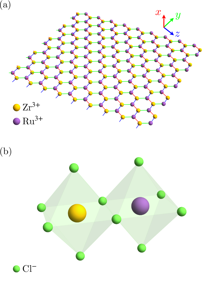
Figure 1: (a) The mixed spin-1/2 and spin-3/2 Kitaev model, where Zr³⁺ and Ru³⁺ ions form a honeycomb lattice (ligand Cl^- ions are not shown) connected by $x$, $y$, and $z$ bonds (red, green, blue) perpendicular to $x$, $y$, and $z$ axis, respectively. (b) The local environment of a bond connected by Zr³⁺ and Ru³⁺ ions, where Zr³⁺ and Ru³⁺ sit in the center of their own octahedral crystal field cage formed by Cl^- ions.

In this work, we investigate the mixed-spin KHM, where spin-1/2 and spin-3/2 ions occupy the A and B honeycomb sublattices. Such mixed spin systems are known from the early days of the theory of Mott insulators, i.e. giving rise to the phenomenon of ferrimagnetism [37, 38], but the realizing of quantum liquids has not been addressed before. Mixing spin-1/2 and spin-3/2 sites within the Kitaev lattice can stabilize unique quantum phases absent in homogeneous systems. For example, introducing a spin-3/2 defect site into a spin-1/2 KHM can act as a magnetic impurity [39], leading to local flux binding effects. These significantly modify the low-energy excitations which offers a new perspective on impurity physics in QSL [39]. Here, we study a homogeneous lattice of mixed spin 1/2 with spin 3/2, which could be potentially realized experimentally in materials such as Zr_0.5Ru_0.5Cl₃ and gives rise to a rich phase diagram with entangled spin and orbital degrees of freedom.

Our main results and the structure of presentation are as follows. In Section II, we describe the derivation of the superexchange theory for Zr_0.5Ru_0.5Cl₃ using the standard strong-coupling approach and identify the necessary conditions for the formation of dominant Kitaev interactions. The technical details are provided in Appendix A. We then sketch the phase diagram of the mixed-spin Kitaev honeycomb model using a combination of parton mean-field theory and DMRG simulations. In Section III.2, we discuss the conserved plaquette operators and propose a reformulation of the model in terms of pseudospin and pseudo-orbital operators. It enables the use of SO(6) Majorana partons to map conserved $Z_{2}$ fluxes onto static $Z_{2}$ gauge fields, facilitating a mean-field analysis in the zero-flux sector. At the mean-field level, four distinct quantum spin liquid (QSL) phases are identified and summarized in the phase diagram shown in Fig. 4. Section IV describes the DMRG approach employed in this study to compute the quadrupolar parameters that differentiate the mean-field QSL phases. Here we also provide a direct comparison between numerical and analytical results, which shows a remarkable quantitative agreement for most of the phase diagram, with the exception of the region near the isotropic point. Finally, Section V discusses the broader significance of our work and highlights potential directions for future research.

II Derivation of the mixed spin superexchange Hamiltonian

A potential candidate material is Zr_0.5Ru_0.5Cl₃ with Ru³⁺ ions in a $d^{5}$ electronic configuration and Zr³⁺ ions in a $d^{1}$ configuration inside Cl^- ion cages forming octahedra, which occupy the two sublattice sites of a honeycomb lattice, see Fig. 1 (a). In the absence of distortions, the Cl^-1 ions form a perfect octahedra cage surrounding the magnetic ion. The octahedral crystal field splits the five $d$ orbitals of both Ru³⁺ and Zr³⁺ into higher-energy doubly-degenerate $e_{g}$ orbitals and lower-energy threefold-degenerate $t_{2g}$ orbitals. Assuming a significant energy gap between the $e_{g}$ and $t_{2g}$ levels for both ions, the five electrons of Ru³⁺ and the single electron of Zr³⁺ are confined to the lower-lying $t_{2g}$ orbitals. Consequently, the key on-site interactions, such as spin-orbit coupling, Coulomb interactions, and Hund’s coupling, are considered within the $t_{2g}$ manifold.

The microscopic Hamiltonian describing this hybrid magnetic ion system can be derived from a three-band Hubbard model, which accounts for the electronic interactions within the $t_{2g}$ orbitals of both Ru³⁺ and Zr³⁺ ions. This approach incorporates the effects of on-site Coulomb interactions, Hund’s coupling, spin-orbit coupling, and hopping processes mediated by the intermediate Cl^- ligands. It is given by

$$\mathcal{H}_{t_{2g}}=\mathcal{H}_{\mathrm{ion}}+\mathcal{H}_{t},$$ (1)

where the single-ion Hamiltonian is given by

$$\mathcal{H}_{\mathrm{ion}}=\sum_{i} \left[U_{1}\sum_{\alpha}n_{i\alpha\uparrow}n_{i\alpha\downarrow}+\frac{1}{2}(U_{2}-J_{H})\sum_{\alpha\neq\alpha^{\prime},\sigma}n_{i\alpha\sigma}n_{i\alpha^{\prime}\sigma}+U_{2}\sum_{\alpha\neq\alpha^{\prime}}n_{i\alpha\uparrow}n_{i\alpha^{\prime}\downarrow}\right.$$

$$+ \left.J_{H}\sum_{\alpha\neq\alpha^{\prime}}d_{i\alpha\uparrow}^{\dagger}d_{i\alpha\downarrow}^{\dagger}d_{i\alpha^{\prime}\downarrow}d_{i\alpha^{\prime}\uparrow}-J_{H}\sum_{\alpha\neq\alpha^{\prime}}d_{i\alpha\uparrow}^{\dagger}d_{i\alpha\downarrow}d_{i\alpha^{\prime}\downarrow}^{\dagger}d_{i\alpha^{\prime}\uparrow}+\mathcal{H}_{i,\mathrm{SOC}}\right],$$ (2)

with $\mathcal{H}_{i,\mathrm{SOC}}$ denoting the spin-orbit coupling on the ion $i$ characterized by the strength $\lambda$, $U_{1}=U_{2}+2J_{H}$ for the cubic $t_{2g}$ orbital, and $\mathcal{H}_{t}$ gives the hopping between the $t_{2g}$ orbitals on Zr and Ru ions. Since Zr and Ru are close in the periodic table, we use the same set of $U_{2}$, $J_{H}$, $\lambda$ for both Zr and Ru.

Noting that the energy of the single-ion Hamiltonian is dominated by the number of electrons occupying the $t_{2g}$ orbital, it would energetically favorable to transfer one electron from the Ru³⁺ ion to the Zr³⁺ ion to minimize the energy of the single-ion Hamiltonian. To avoid this situation, which is magnetically inert, we introduce a positive onsite potential energy $V$ on the Zr³⁺ ions to stabilize the ground state of the Zr–Ru system in the desired $d^{1}$–$d^{5}$ configuration. We assume $V$ to be large enough that the $d^{1}$–$d^{5}$ configuration will be the ground state of the system, but not so large as to favor the $d^{0}$–$d^{6}$ configuration. The acceptable range for $V$ is given by: $\frac{1}{4}(12U_{2}-6J_{H}-3\lambda+\sqrt{16J_{H}^{2}+8J_{H}\lambda+9\lambda^{2}}+2\sqrt{25J_{H}^{2}+10J_{H}\lambda+9\lambda^{2}})<V<5U_{2}+\frac{3\lambda}{2}$. For reasonable parameters, such as $U_{2}=2.0$ eV, $J_{H}=0.4$ eV, and $\lambda=0.15$ eV, we find that $7~\mathrm{eV}\lesssim V\lesssim 10~\mathrm{eV}$. Whether this can be achieved in actual materials needs to be investigated with more sophisticated ab-initio and quantum chemistry methods, but, at the very least, our perturbative calculations below confirm as a proof of principle how a mixed spin KHM can emerge as an effective low energy description.

The stabilized $d^{1}$–$d^{5}$ electronic configuration results in a ground-state manifold described by the effective spin states $|J^{z}_{J=3/2},J^{z}_{J=1/2}\rangle$. Assuming that the mixed spin-1/2 and spin-3/2 system remains insulating, we model the virtual electron hoppings using $\mathcal{H}_{t}$. By treating the hopping of electrons between the $t_{2g}$ orbitals as a perturbation, we derive the superexchange Hamiltonian in the basis of $|J^{z}_{J=3/2},J^{z}_{J=1/2}\rangle$, which takes the form:

$$\mathcal{H}_{\mathrm{eff},ij}=\sum_{n,m}^{8}\sum_{\mathrm{excited}}\frac{\langle n_{i}|\mathcal{H}_{t}|\mathrm{excited}\rangle\langle\mathrm{excited}|\mathcal{H}_{t}|m_{j}\rangle}{E_{\mathrm{Zr}}^{(0)}+E_{\mathrm{Ru}}^{(0)}-(E_{\mathrm{excited}}\pm V)}|n_{i}\rangle\langle m_{j}|,$$ (3)

where $n_{i}$, $m_{j}$ denotes $n$-th, $m$-th state from the $|J^{z}_{J=3/2}J^{z}_{J=1/2}\rangle$ basis on site $i$ and $j$ respectively, $E_{\mathrm{Zr}}^{(0)}$, $E_{\mathrm{Ru}}^{(0)}$ are the ground state energies of the single-ion Hamiltonian, and $E_{\mathrm{excited}}\pm V$ corresponds to the energy of the excited state with the sign $\pm$ depending on the excited electronic configuration, $d^{2}$–$d^{4}$ or $d^{0}$–$d^{6}$.

The resulting superexchange Hamiltonian on the $z$ bond is expressed as a product of orthogonal spin-3/2 and spin-1/2 operators, with the corresponding coupling strengths detailed in Table 1. This formulation captures the anisotropic nature of the interactions arising from the underlying spin-orbital coupling and crystal field effects. In addition to these interactions, the perturbative calculations also introduce single-ion anisotropy terms for the spin-3/2 degrees of freedom, as shown in Table 2. Specifically, the $D_{i}$ represents dipole-dipole interactions between spin-1/2 and spin-3/2 moments, while the $O_{i}$ terms correspond to the couplings associated with the higher-order interactions. The $Q_{i}$ terms account for contributions from single-ion anisotropy.

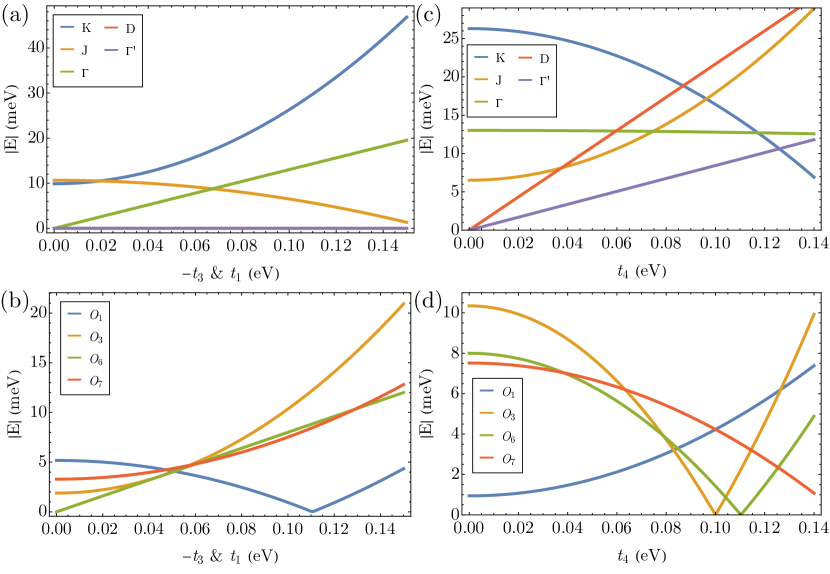
Figure 2: Superexchange interactions for the mixed spin-1/2–spin-3/2 system. The parameters are fixed as $U_{2}=2$ eV, $J_{H}=0.4$ eV, and $\lambda=0.15$ eV. In panels (a) and (c), we show the dipole-dipole couplings $J$, $K$, $\Gamma$, $\Gamma^{\prime}$, and $D$. In panels (b) and (d), the largest higher-order interactions, $O_{1}$, $O_{3}$, $O_{6}$, and $O_{7}$, are presented. For panels (a) and (b), the hopping parameters are set as $t_{2}=0.114$ eV and $t_{4}=0$ eV, while $t_{1}=-t_{3}$ is varied from 0 to 0.15 eV. In panels (c) and (d), we fix $t_{2}=0.114$ eV and $t_{1}=-t_{3}=0.1$ eV, and vary $t_{4}$ from 0 to 0.15 eV.

	$S_{x}$	$S_{y}$	$S_{z}$
$J_{x}$	$D_{1}$	$D_{2}$	$D_{4}$
$J_{y}$	$D_{2}$	$D_{1}$	$D_{4}$
$J_{z}$	$D_{4}^{\prime}$	$D_{4}^{\prime}$	$D_{3}$
$(J^{x})^{3}$	$O_{1}$	$O_{2}$	$O_{4}$
$(J^{y})^{3}$	$O_{2}$	$O_{1}$	$O_{4}$
$(J^{z})^{3}$	$O_{4}^{\prime}$	$O_{4}^{\prime}$	$O_{3}$
$J^{x}J^{y}J^{z}+J^{z}J^{y}J^{x}$	$O_{5}$	$O_{5}$	$O_{6}$
$J^{x}J^{z}J^{z}-J^{y}J^{y}J^{x}$	$O_{7}$	$O_{8}$	$O_{9}$
$J^{y}J^{z}J^{z}-J^{x}J^{x}J^{y}$	$O_{8}$	$O_{7}$	$O_{9}$
$J^{y}J^{y}J^{z}-J^{z}J^{x}J^{x}$	$O_{10}$	$-O_{10}$	$O_{11}$

Table 1: Superexchange coupling constants between spin-3/2 and spin-1/2 degrees of freedom on the $z$ bond.

$-2J^{x}J^{x}+J^{y}J^{y}+J^{z}J^{z}$	$Q_{1}$
$J^{z}J^{z}-J^{y}J^{y}$	$Q_{2}$
$J^{x}J^{y}+J^{y}J^{x}$	$Q_{3}$
$J^{x}J^{z}+J^{z}J^{x}$	$Q_{4}$
$J^{y}J^{z}+J^{z}J^{y}$	$Q_{4}$

.

Table 2: Single ion anisotropy for spin-3/2 degrees of freedom induced by the hopping on the $z$ bond.

Focusing on the dipole-dipole couplings between the spin-1/2 and spin-3/2 moments, we rewrite these matrices in a familiar format commonly used for Kitaev materials. In this notation, we assign $J=D_{1}$, $K=D_{3}$, $\Gamma=D_{2}$, and $\Gamma^{\prime}+D=D_{4}$ for the dipole-dipole couplings, and $\Gamma^{\prime}-D=D_{4}^{\prime}$ for other interactions. Here $D$ denotes the Dzyaloshinskii-Moriya interaction. With these definitions, the effective Hamiltonian on the $z$-bond can be expressed as:

$$\begin{array}[]{l}\mathcal{H}_{ij,z}\!=\!J{\bf S}_{i}\!\cdot\!{\bf J}_{j}\!+\!KS^{z}_{i}J^{z}_{j}\!+\!\Gamma(S^{x}_{i}J^{y}_{j}\!+\!S^{y}_{i}J^{x}_{j})\\ ~~~~~~+\Gamma^{\prime}\big{(}S^{x}_{i}J^{z}_{j}+S^{z}_{i}J^{x}_{j}+S^{y}_{i}J^{z}_{j}+S^{z}_{i}J^{y}_{j}\big{)}\\ ~~~~~~+D\big{(}S^{x}_{i}J^{z}_{j}-S^{z}_{i}J^{x}_{j}+S^{y}_{i}J^{z}_{j}-S^{z}_{i}J^{y}_{j}\big{)}+...\,,\end{array}$$ (7)

where $...$ includes terms for higher-order interactions and single-ion anisotropy contributions.

We first numerically examine these coupling constants by using parameters typically associated with $\alpha$-RuCl₃: $U_{2}=2$ eV, $J_{H}=0.4$ eV, $\lambda=0.15$ eV, and the hopping parameters $t_{1}=0.066$ eV, $t_{2}=0.114$ eV, $t_{3}=-0.229$ eV, and $t_{4}=-0.010$ eV. We also assume an onsite potential of $V=8$ eV for the Zr ions. It provides an estimate for the strength of the superexchange coupling constants, which are presented in Table 4 of Appendix A. While these parameters give a dominant Kitaev interaction, there are still sizable contributions from the non-Kitaev exchanges.

To explore whether it is possible to further maximize the Kitaev interaction while suppressing non-Kitaev terms, we systematically vary these parameters. Clearly, real hopping parameters in any mixed spin-1/2–spin-3/2 system are expected to differ from those of $\alpha$-RuCl₃ due to the mixed-spin configuration and potential lattice distortions. To account for this, we systematically vary these parameters to identify an optimal set that enhances the Kitaev interaction and ensures it dominates over competing terms.

As a starting point, we fix all parameters to their $\alpha$-RuCl₃ values but set $t_{4}=0$ eV and impose $t_{1}=-t_{3}$. We then vary $t_{1}$ from 0 to 0.15 eV to explore the parameter space for maximizing the Kitaev interaction. The resulting couplings are shown in Fig. 2 (a) and (b). We observe that for $t_{1}=-t_{3}$ in the range of 0.04 to 0.1 eV, the Kitaev interaction is the largest coupling, ranging from 12 to 20 meV. However, other interactions remain significant. For instance, the $\Gamma$ interaction is approximately half the strength of the Kitaev interaction, and several higher-order terms, such as $O_{3}$, $O_{6}$, and $O_{7}$, also contribute significantly to the overall coupling landscape.

Next, we fix $t_{2}=0.114$ eV and $t_{1}=-t_{3}=0.1$ eV, and vary $t_{4}$ from 0 to 0.15 eV. The resulting couplings are shown in Fig. 2 (c) and (d). Our results show that increasing the $t_{4}$ hopping reduces the Kitaev interaction while simultaneously increasing the Heisenberg coupling $J$ and, in particular, the Dzyaloshinskii-Moriya interaction $D$.

To conclude this section, we note that in the case of an ideal structure, the three bond types—$x$, $y$, and $z$—are related by $C_{3}$ rotational symmetry. As a result, it can be shown that the contributions from the single-ion anisotropy terms $Q_{1}$ and $Q_{2}$ sum to zero when contributions from all three bonds are considered. While the single-ion anisotropy terms $Q_{3}$ and $Q_{4}$ contribute non-zero terms, they remain subdominant across the entire range of hopping parameters considered, which is why they are not shown here.

III Mixed-spin Kitaev Honeycomb Model

After having established a microscopic setting how a mixed-spin 1/2 and spin 3/2 KHM can emerge, we next address the question of what quantum phases can be realized. We expect a very complex phase diagram comprising not only the different long-range spin ordered phases induced by the non-Kitaev exchanges known from the spin 1/2 extended KHM, but in addition, long-range quadrupole orders. To make progress, in this section we focus on the sought-after QSL regime and study a limiting case where the Kitaev interaction $K$ is dominant, which is a plausible scenario for a reasonable set of microscopic parameters.

To facilitate the analysis, we examine the mixed-spin 3/2–1/2 Kitaev model, introducing a single-ion anisotropy (SIA) term. This addition allows for a more manageable investigation while retaining the essential features of the mixed-spin KHM. As in previous studies of higher-spin KHMs, the system is no longer exactly solvable, even for pure Kitaev exchange, making understanding its QSL phases a formidable task in itself [21].

III.1 Exact results and conserved fluxes

Specifically, we focus on the following Hamiltonian:

$$H=\sum_{\left\langle ij\right\rangle_{\gamma}}K_{\gamma}S_{i}^{\gamma}J_{j}^{\gamma}+H_{\text{SIA}},$$ (8)

where $\gamma$ simultaneously labels the quantization axes and the distinct bond directions. The simplest SIA term is

$$H_{\text{SIA}}=D_{z}\sum_{j}\left(J_{j}^{z}\right)^{2},$$ (9)

which lifts the four-fold degeneracy of $J=3/2$ quadruplet by splitting $J_{z}=\pm 3/2$ and $J_{z}=\pm 1/2$ levels.

The local symmetries of Eq. (8) can be made more transparent in terms of $J=3/2$ pseudospin and pseudo-orbital operators [21, 22]. We introduce the pseudospins by

$$\sigma_{l}^{\gamma}=-i\exp\left(i\pi J_{l}^{\gamma}\right),$$ (10)

which corresponds to the local operators forming the spin-$S$ conserved quantities [19]. Likewise, the pseudo-orbital operators read

$$T_{j}^{z}=\left(J_{j}^{z}\right)^{2}-5/4,$$

$$T_{j}^{x}=\frac{1}{\sqrt{3}}\left[\left(J_{j}^{x}\right)^{2}-\left(J_{j}^{y}\right)^{2}\right],$$

$$T_{j}^{y}=\frac{2\sqrt{3}}{9}\overline{J_{j}^{x}J_{j}^{y}J_{j}^{z}},$$ (11)

where the bar indicates the sum over all possible permutations. The operators $\left(T^{z},T^{x}\right)$ are quadrupoles that transform as $e_{g}$ orbital operators under real-space rotations. By contrast, the octupolar operator $T^{y}$ forms a one-dimensional representation of the $O_{h}$ symmetry group [36]. In conjunction, $\bm{\sigma}$ and $\bf{T}$ satisfy the algebra

$$\left[\sigma_{i}^{\alpha},\sigma_{j}^{\beta}\right] =2i\delta_{ij}\epsilon^{\alpha\beta\gamma}\sigma_{i}^{\gamma},$$

$$\left[T_{i}^{\alpha},T_{j}^{\beta}\right] =2i\delta_{ij}\epsilon^{\alpha\beta\gamma}T_{i}^{\gamma},$$

$$\left\{\sigma_{i}^{\alpha},\sigma_{j}^{\beta}\right\} =\left\{T_{i}^{\alpha},T_{j}^{\beta}\right\}=2\delta_{ij}\delta^{\alpha\beta},$$

$$\left[\sigma_{i}^{\alpha},T_{j}^{\beta}\right] =0.$$ (12)

The fifteen operators $\left\{\sigma^{a},T^{b},\sigma^{a}T^{b}\right\}$ correspond to generators of SU(4), implying that they can be used to rewrite any Hermitian $J=3/2$ operator. A simple example is Eq. (9), which reads

$$H_{\text{SIA}}=D_{z}\sum_{j}T_{j}^{z}+\text{const}.$$ (13)

We can also write $J_{i}^{\gamma}$ as [21, 22]

$$J_{i}^{\gamma}=-\frac{\sigma_{i}^{\gamma}}{2}-\sigma_{i}^{\gamma}T_{i}^{\alpha\beta},$$ (14)

where the compass-like pseudo-orbitals $T^{\alpha\beta}$ are

$$T_{i}^{xy}=T_{i}^{z},\quad T_{i}^{yz(zx)}=-\frac{T_{i}^{z}}{2}\pm\frac{\sqrt{3}T_{i}^{x}}{2}.$$ (15)

The mixed-spin exchange model in Eq. (8) is then rewritten as

$$H_{\text{K}}=\sum_{\left\langle ij\right\rangle_{\gamma}}K_{\gamma}S_{i}^{\gamma}\sigma_{j}^{\gamma}\left(\frac{1}{2}+T_{j}^{\alpha\beta}\right).$$ (16)

Crucially, it allows us to show that the Hamiltonian commutes with the local plaquette operators

$$W_{p}=2^{3}S^{z}_{1}\sigma^{x}_{2}S^{y}_{3}\sigma^{z}_{4}S^{x}_{5}\sigma^{y}_{6},$$ (17)

in which the quantization axes correspond to the outward bond label. The presence of a conserved plaquette flux is in close analogy with the spin-1/2 [2] and spin-3/2 KHM [19, 21, 22]. The multiplying factor $2^{3}$ was introduced to ensure the $W_{p}$ eigenvalues are $\pm 1$. The extensive number of conserved quantities indicates that the model realizes a Kitaev QSL and is amenable to an analytical treatment, as we will show in the following section. These conserved quantities also provide guidelines for interpreting the DMRG results, as explored in Section IV.

The SIA term in Eq. (9) and $W_{p}$ also commute which follows directly from the commutation relations between $T^{z}$ and $\bm{\sigma}$, allowing us to use it as a control parameter. In the $D_{z}\rightarrow+\infty$ limit, pseudo-orbital fluctuations are effectively suppressed, allowing us to fix $T^{z}=-1$ and to project the $J^{\gamma}$ angular momenta onto the pseudospins according to the rule:

$$\left(J_{j}^{x},J_{j}^{y},J_{j}^{z}\right)\overset{D_{z}\rightarrow+\infty}{\longrightarrow}\left(-2\sigma^{x},-2\sigma^{y},\sigma^{z}\right).$$ (18)

Therefore, Eq. (8) reduces to

$$\lim_{D_{z}\rightarrow\infty}H=\sum_{\left\langle ij\right\rangle_{\gamma}}K_{\gamma}^{\prime}S_{i}^{\gamma}\sigma_{j}^{\gamma}.$$ (19)

with modified coupling constants $\left(K_{x}^{\prime},K_{y}^{\prime},K_{z}^{\prime}\right)=\left(-2K_{x},-2K_{y},K_{z}\right)$. Fixing $T^{z}=-1$ implies that $\sigma^{\gamma}$ will act on the $J^{z}=\pm 1/2$ manifold only, allowing the pseudospins to be treated as effective spin-1/2 operators. Thus, the SIA connects the mixed-spin KHM model to the standard spin-1/2 KHM, therefore introducing an exactly solvable limit.

III.2 Majorana representation and parton mean-field theory

An analytical treatment of the mixed-spin KHM becomes possible by introducing Majorana partons, which map $Z_{2}$ conserved quantities in Eq. (17) onto fluxes of a static $Z_{2}$ gauge field. We begin by representing the spin-1/2 degrees of freedom using the Kitaev Majorana parton framework [2]:

$$S_{i}^{\gamma}=-\frac{i}{2}\eta_{i}^{\gamma}c_{i},$$ (20)

in which all Majorana particles with flavors $\xi^{\alpha}$ at sites $i,j$ satisfy

$$\left\{\xi_{i}^{\alpha},\xi_{j}^{\beta}\right\}=2\delta_{ij}\delta^{\alpha\beta}.$$ (21)

Likewise, we introduce the SO(6) Majorana representation for spin-3/2 as follows [21, 22, 40]

$$\bm{\sigma}_{i}=-\frac{i}{2}\bm{\eta}_{i}\times\bm{\eta}_{i}, \,\mathbf{T}_{i}=-\frac{i}{2}\bm{\theta}_{i}\times\bm{\theta}_{i},$$

$$\sigma_{i}^{\alpha}T_{i}^{\beta} =-i\eta_{i}^{\alpha}\theta_{i}^{\beta}.$$ (22)

The first two equations correspond to the SO(3) Majorana representation of spin-1/2 systems [41, 42] and reproduce the algebra from Eq. (12). The second line allows us to represent all spin-orbital operators as bilinears and is consistent with the constraint on the physical Hilbert space

$${\mathcal{D}}_{i}=i\eta_{i}^{\alpha}\eta_{i}^{\beta}\eta_{i}^{\gamma}\theta_{i}^{\alpha}\theta_{i}^{\beta}\theta_{i}^{\gamma}=1.$$ (23)

The ${\mathcal{D}}_{i}$ operator not only enforces the constraint but also provides an alternative representation of the pseudospin operators as quartic operators, as discussed in recent studies [21, 22, 43]:

$$\sigma_{j}^{\gamma}=-\frac{i}{2}\eta_{j}^{\gamma}\theta_{j}^{0},$$ (24)

where $\theta_{j}^{0}\equiv-i\theta_{j}^{x}\theta_{j}^{y}\theta_{j}^{z}$.

The Hamiltonian in Eq. (8), expressed in the Majorana parton representation, takes the form:

$$H =\frac{1}{4}\sum_{\left\langle ij\right\rangle_{\gamma}}K_{\gamma}\hat{u}_{\left\langle ij\right\rangle_{\gamma}}ic_{i}\left(\theta_{j}^{0}+2\theta_{j}^{\alpha\beta}\right)$$

$$-D_{z}\sum_{j}i\theta_{j}^{x}\theta_{j}^{y},$$ (25)

in which $\hat{u}_{\left\langle ij\right\rangle_{\gamma}}=-i\eta_{i}^{\gamma}\eta_{j}^{\gamma}$ represents a static $Z_{2}$ gauge operator. Replacing $\left\{\hat{u}_{\left\langle ij\right\rangle_{\gamma}}\right\}$ by their $\pm 1$ eigenvalues determines the flux sectors labeled by $W_{p}$. The zero-flux sector ($W_{p}=+1,\forall p$) is the ground state of the Kitaev spin-1/2 model, as established by Lieb’s theorem [44]. Additionally, both numerical and analytical studies provide strong evidence that this sector also hosts the ground state of the KHM for arbitrary spin-$S$ [19, 20, 21, 22]. Thus, we will focus on the zero-flux sector of the mixed-spin KHM, a choice further supported by the DMRG simulations presented later in this work.

The Hamiltonian in Eq. (25), after gauge fixing, consists of Majorana bilinear terms with additional quartic interactions of the form $ic_{i}\theta_{j}^{0}$, which requires a mean-field treatment. The most general mean-field decoupling within a fixed gauge sector can be expressed as:

$$ic_{i}\theta_{j}^{0} \approx\Delta_{\left\langle ij\right\rangle_{\gamma}}^{x}i\theta_{j}^{y}\theta_{j}^{z}+\Delta_{\left\langle ij\right\rangle_{\gamma}}^{y}i\theta_{j}^{z}\theta_{j}^{x}+\Delta_{\left\langle ij\right\rangle_{\gamma}}^{z}i\theta_{j}^{x}\theta_{j}^{y}$$

$$+Q_{j}^{x}ic_{i}\theta_{j}^{x}+Q_{j}^{y}ic_{i}\theta_{j}^{y}+Q_{j}^{z}ic_{i}\theta_{j}^{z},$$ (26)

in which the parameters are defined by

$$\Delta_{\left\langle ij\right\rangle_{\gamma}}^{t} =-\left\langle ic_{i}\theta_{j}^{t}\right\rangle$$

$$Q_{j}^{t} =\left\langle T_{j}^{t}\right\rangle=-\left\langle i\theta_{j}^{r}\theta_{j}^{s}\right\rangle,$$ (27)

in which $\left\langle\hat{O}\right\rangle$ is the ground state expectation value of $\hat{O}$. The zero-flux sector is obtained after fixing $u_{\left\langle ij\right\rangle_{\gamma}}=+1$. It is convenient to distinguish between sites $\mathbf{r}$, which host spin-1/2 ions, and their neighboring sites $\mathbf{r}_{\gamma}$, which host spin-3/2 ions. The mean-field decoupled Hamiltonian then reads:

$$H_{\text{MFT}} =\frac{1}{2}\sum_{\mathbf{r},\gamma}K_{\gamma}ic_{\mathbf{r}}\theta_{\mathbf{r}_{\gamma}}^{\alpha\beta}$$

$$+\frac{1}{4}\sum_{\mathbf{r},\gamma,t}K_{\gamma}Q^{t}ic_{\mathbf{r}}\theta_{\mathbf{r}_{\gamma}}^{t}$$

$$+\frac{1}{4}\sum_{\mathbf{r},\gamma,t}K_{\gamma}\Delta_{\gamma}^{t}i\theta_{\mathbf{r}_{\gamma}}^{r}\theta_{\mathbf{r}_{\gamma}}^{s}$$

$$-D_{z}\sum_{\mathbf{r}_{\gamma}}i\theta_{\mathbf{r}_{\gamma}}^{x}\theta_{\mathbf{r}_{\gamma}}^{y},$$ (28)

in which we fixed $\epsilon^{rst}=1$ and used the translational invariance to simplify the mean-field parameters. The mean-field Hamiltonian can be conveniently rewritten in the Fourier space as

$$H_{\text{MFT}} =\sum_{\mathbf{k}}\Psi_{\mathbf{k}}^{\dagger}H_{\mathbf{k}}\Psi_{\mathbf{k}}$$

$$=\sum_{\mathbf{k}}\Phi_{\mathbf{k}}^{\dagger}(U_{\mathbf{k}}^{\dagger}H_{\mathbf{k}}U_{\mathbf{k}})\Phi_{\mathbf{k}}$$

$$\equiv\sum_{\mathbf{k}}\Phi_{\mathbf{k}}^{\dagger}\Omega_{\mathbf{k}}\Phi_{\mathbf{k}},$$ (29)

where $\Psi_{\mathbf{k}}^{\dagger}$ is a row vector of four canonical fermion operators, $\Phi_{\mathbf{k}}^{\dagger}=\Psi_{\mathbf{k}}^{\dagger}U_{\mathbf{k}}$ are the eigenstates, and $\Omega_{\mathbf{k}}=U_{\mathbf{k}}^{\dagger}H_{\mathbf{k}}U_{\mathbf{k}}$ is the diagonal matrix of eigenvalues. The mean-field ground state $\left|\Psi_{0}\right\rangle$ satisfies $\Phi_{\mathbf{k}}\left|\Psi_{0}\right\rangle=0$ for all $\Phi_{\mathbf{k}}$ corresponding to negative eigenstates.

The self-consistency algorithm begins with an initial guess $\mathbf{x}_{0}=\left(\Delta_{\gamma}^{x},..,Q^{z}\right)$ for the order parameters. This initial guess defines the starting Hamiltonian and determines the unitary matrices $U_{\mathbf{k}}$. The initial guess also allows us to evaluate a vector $\mathbf{x}_{\text{par}}(\mathbf{x})$ using Eq. (27). The self-consistent condition can then be reformulated as a root-finding problem for the function $f(\mathbf{x})=\mathbf{x}_{\text{par}}(\mathbf{x})-\mathbf{x}$. Such problems are efficiently solved using standard algorithms such as Broyden’s method [45]. For concreteness, we considered self-consistent solutions $\left|f(\mathbf{x})\right|<\text{tol}$, in which the tolerance was of the order $10^{-12}$. The algorithm was run with $\sim 200$ initial guesses $\mathbf{x}_{0}$ to ensure that all self-consistent solutions could be found.

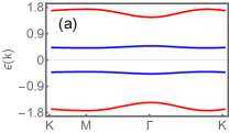
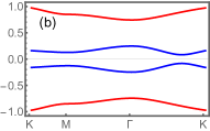
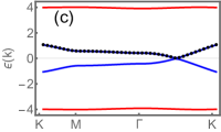
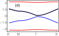
Figure 3: Dispersion of the Majorana bands for representative mean-field ground states obtained for fixed $K_{x}=K_{y}=1$. (a) $K_{z}=2$, $D_{z}=0$, representing the gapped $B$ phase with $Q^{z}>0$, $Q^{x}=0$, (b) $K_{z}=0.5$, $D_{z}=0$ representing the twofold degenerate $C$ phase with $Q^{z}<0$, $Q^{x}\neq 0$, (c) $K_{z}=2.3$, $D_{z}=4$, representing a spin liquid with $Q^{z}\approx-1$ adiabatically connected to the gapless Kitaev spin liquid $A_{0}$, (d) $K_{z}=4.5$, $D_{z}=4$ represents a spin liquid with $Q^{z}\approx-1$ adiabatically connected to the gapped Kitaev spin liquid $A_{z}$. The black points on the figure corresponds to the exact Majorana dispersion of the spin-1/2 KHM with modified coupling constants $\left(K_{x}^{\prime},K_{y}^{\prime},K_{z}^{\prime}\right)=\left(-2K_{x},-2K_{y},K_{z}\right)$.

The mean-field ground state is determined by the self-consistent solution $\mathbf{x}$ that minimizes the ground-state energy:

$$E_{\text{GS}}=\sum_{\mathbf{k},\Omega_{\mathbf{k},a}<0}\Omega_{\mathbf{k},a}.$$ (30)

Fig. 3 illustrates some representative dispersions for fixed coupling constants $K_{x}=K_{y}=1$ but varying $K_{z}$ and $D_{z}$ values. For all the parameters examined, we found $Q^{y}=0$, which implies that time-reversal invariance is preserved. Figs. 3(a) and 3(b) display gapped spin liquids in the small single-ion anisotropy limit (in this case, we set $D_{z}=0$) that are physically distinguished by the order parameters $Q^{z}$ and $Q^{x}$. Fig. 3(a) displays a $K_{z}>1$ case, for which the gapped liquid $B$ is unique and characterized by $Q^{z}>0$ and $Q_{x}=0$. This is analogous to the toric-code phase, being described in terms of dimers on the $z-$bonds containing $S^{z}=\pm 3/2$ states. Fig. 3(b) displays the dispersion of a twofold degenerate gapped liquid $C$ that is stabilized when $K_{z}<1$. This phase is characterized by $Q^{z}<0$ and $Q_{x}\neq 0$, where $Q_{x}$ can take two values of equal magnitude but opposite sign.

At the isotropic point $K_{z}=1$ and $D_{z}=0$, the mean-field theory indicates a three-fold degeneracy corresponding to the $B$ and $C$ spin liquids. More explicitly, this solution is characterized by

$$(Q^{z},Q^{x})_{\text{MFT}} = 0.845(1,0)$$

$$(Q^{z},Q^{x})_{\text{MFT}} = 0.845\left(-\frac{1}{2},\pm\frac{\sqrt{3}}{2}\right).$$ (31)

This result should be compared with the spin-3/2 KHM, for which this point is critical and characterized by vanishing quadrupolar parameters, thereby characterizing it as a QSOL [21, 22]. By contrast, the isotropic mixed-spin KHM is characterized by a level crossing between two possible mean-field states. A comparison between this result and the one obtained through DMRG will be given in the next section.

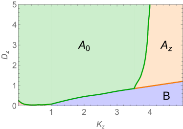
Figure 4: Mean-field phase diagram showing the quantum spin liquids hosted by the mixed-spin Kitaev model. The phases $A_{0}$, $A_{z}$, and $B$ occupy the largest area of the diagram. The phase $C$ occupies a small area of the diagram with small $D_{z}$ and $0<K_{z}<1$.

Turning on the SIA connects the mixed-spin and the $S=1/2$ KHM, providing a regime in which the mean-field theory recovers known exact results. Figs. 3 (c) and (d) illustrate two cases in the large SIA limit, where the parameter $Q^{z}$ is very close to -1. In this limit, both the gapless ($A_{0}$) and gapped ($A_{z}$) phases are adiabatically connected to the $S=1/2$ Kitaev QSL. This connection is explicitly demonstrated by the agreement between the mean-field low-energy bands and the exact Majorana fermion dispersion of the $S=1/2$ KHM with appropriately modified coupling constants [2]. The full phase diagram of the model (8) is displayed in Fig. 4. It reveals the dominance of the $B$, $A_{0}$, and $A_{z}$ phases across most of the parameter space, with the $C$ phase occupying only a narrow region when $0<K_{z}<1$.

IV Numerical simulations

To examine the validity and robustness of our parton mean-field theory, we perform state-of-the-art density matrix renormalization group (DMRG) simulations  [46, 47] to investigate the ground state of Hamiltonian  (8). These calculations are performed on a two-dimensional honeycomb lattice comprising $L_{y}\times L_{x}$ unit cells, arranged in a cylindrical geometry. Periodic boundary conditions (PBC) are applied along the shorter dimension (circumference $L_{x}$), while the longer dimension (length $L_{y}$) remains open. This cylindrical setup explicitly breaks the $C_{3}$ rotational symmetry of the lattice. To ensure high numerical accuracy, we use a bond dimension of up to $\chi=4000$, achieving a typical truncation error of approximately $\epsilon\simeq 10^{-6}$.

The ground states obtained by DMRG simulations exhibit a zero-flux configuration in both the $A_{0}$ and $A_{z}$ phases in accordance with our Ansatz. In the $B$ phase, however, our DMRG simulations do not converge to a unique ground-state flux configuration. Instead, they yield a disordered-flux state, where the flux on each plaquette deviates from the expected values of $1$ or $-1$. This behavior is reminiscent of findings in a previous study on the $S=3/2$ Kitaev honeycomb model [21], where this phenomenon was attributed to an extremely small energy gap associated with $Z_{2}$ flux flipping in the $B$ phase.

We also calculate the averaged expectation values of $J=3/2$ multipole operators $Q^{z}=\langle{}T^{z}\rangle$ and $Q^{x}=\langle{}T^{x}\rangle$. These two values are spatially uniform in the bulk of cylinders and are qualitatively consistent with the parton mean-field theory, as demonstrated by the data in Table 3 and Fig. 6.

Table 3: Averaged expectation values of $Q^{z}=\langle{}T^{z}\rangle$ and $Q^{x}=\langle{}T^{x}\rangle$, as well as ground-state flux configurations. The data is obtained on a cylinder with $L_{y}=4$ and $L_{x}=12$.

($K_{z}$, $D_{z}$)	$Q^{z}$	$Q^{x}$	zero-flux
(1.1, 0.0)	0.84	-1e-5	No
(1.05,0.0)	0.82	-5e-5	No
(1.0, 0.05)	-0.69	0.25	Yes
(1.0, 0.1)	-0.75	0.12	Yes
(1.0, 0.2)	-0.8	0.05	Yes
(1.0, 0.3)	-0.86	0.02	Yes
(1.0, 1.0)	-0.94	0.01	Yes
(3.0, 1.0)	-0.90	0.02	Yes
(3.6, 1.0)	-0.89	0.01	Yes
(3.8, 1.0)	-0.88	0.01	Yes
(4.4, 1.0)	-0.87	0.01	Yes
(4.6, 1.0)	0.985	-2e-5	No
(5.0, 1.0)	0.988	1e-7	No

For the isotropic point of $K_{z}=1$ and $D_{z}=0$, we use exact diagonalization to calculate the ground state on a torus. To preserve the $C_{3}$ rotational symmetry, we consider a 24 lattice-site cluster shown in Fig. 5. Note that this cluster geometry breaks the translation symmetries in both directions. We implement the $Z_{2}$ flux conservation (e.g., a local symmetry) with the QuSpin package [48]. Focusing on the zero-flux sector, we find that the ground states exhibit a 3-fold degeneracy for the $C_{3}$ rotational symmetry in which the expectation values of $T^{z}$ and $T^{x}$ operators manifest exactly the same relative values as those predicted by the parton mean-field theory, namely,

$$(Q^{z},Q^{x})_{\text{MFT}} = (-0.1214,0)$$

$$(Q^{z},Q^{x})_{\text{MFT}} = (+0.0607,0.1051)$$ (32)

$$(Q^{z},Q^{x})_{\text{MFT}} = (+0.0607,-0.1051)$$

Moreover, we find that the first excited states in the zero-flux sector also display the same 3-fold degeneracy.

Comparing the DMRG results with the mean-field results at the isotropic point Eq.(31) shows a qualitative agreement with respect to the relative values of $Q^{x}$ and $Q^{z}$, but a strong quantitative disagreement. We explore the nature of this disagreement in Fig. 6(a) by first fixing the value $K_{z}=1$ and varying the SIA. Starting at large values of $D_{z}$, we observe a strong quantitative agreement between the two techniques for both order parameters up to $D_{z}\sim 0.1$. Below this range, there is a sizable divergence between the computed parameters, specially for $Q^{x}$. Fig. 6(b) indicates a complementary analysis in which $D_{z}=1$ is fixed in order to ensure only the $A_{0}$ and $A_{z}$ phases. The quantitative agreement between the evaluated parameters is recovered, even concerning the location of the phase transition.

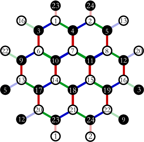
Figure 5: A 24 lattice-site cluster with $C_{3}$ rotational symmetry. The white and black dots the $S=1/2$ and $J=3/2$ spins, respectively. The blue, green, and red bonds represent the $x-$, $y-$, and $z-$type bonds. The transparent bonds denote the boundary bonds.

Our analysis indicates that mean-field theory and DMRG will converge to the same kind of spin liquids except in the neighborhood of the isotropic point, namely, parton mean-field theory converges to the $B$ or $C$ phases that are continuously connected to the same spin liquids at $K_{z}>1$ and $K_{z}<1$. On the other hand, DMRG and exact diagonalization predict a sign inversion of the $Q^{z}$ order parameter leading to a qualitatively different spin liquid in this region. Furthermore, this parameter will display a reduced absolute value, but not a vanishing one as observed for the spin-3/2 KHM [21, 22], a feature that cannot be explained by $C_{3}$ symmetry constraints [22]. The nature of the isotropic mixed-spin Kitaev spin liquid also differs from the large-$S$ Kitaev spin liquids [20], since the quadrupolar parameters preserve translational symmetry. Thus, the mixed-spin model stabilizes a qualitatively different QSL, whose nature is not yet tractable within our parton Ansatz.

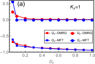
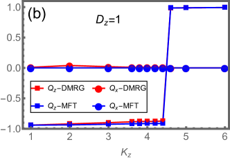
Figure 6: Comparison between computed order parameters using parton mean-field theory (in blue) and DMRG (in red). The $Q^{z}$ order parameter is indicated with squares, while $Q^{x}$ is displayed with circles. Fig. (a) investigates the parameters with fixed exchange $K_{z}=1$ but varying $D_{z}$. In (b), the single-ion anisotropy is fixed at $D_{z}=1$, but the $K_{z}$ is varied over values such

V Conclusions

In this work, we explored the mixed-spin Kitaev honeycomb model, where alternating spin-1/2 and spin-3/2 ions occupy the two sublattice positions of the honeycomb lattice. We focused on a potential experimental realization in materials such as Zr_0.5Ru_0.5Cl₃ and a theoretical understanding of the ensuing QSL phases. We derived a microscopic superexchange Hamiltonian and identified conditions under which dominant Kitaev-like interactions arise. In the regime with pure Kitaev interactions and single-ion anisotropy, we constructed a comprehensive phase diagram using parton mean-field theory and DMRG simulations. The phase diagram reveals four distinct QSL phases, each characterized by a unique quadrupolar order parameter, specific flux configurations, and Majorana fermion excitations. The quantitative agreement between parton mean-field analysis and numerical approaches highlights the robustness of our framework, except in a small parameter region around the isotropic point.

While our study focused on pure Kitaev interactions with single-ion anisotropy, taking into account other interactions in Eq.(7), such as the Heisenberg exchange, bond-anisotropic $\Gamma$-interaction, and higher-order multipolar couplings, could stabilize other exotic phases, including chiral QSLs and magnetically ordered states. These extensions provide further opportunities for future research to explore the interplay between dipolar and multipolar interactions, potentially uncovering an even broader spectrum of quantum phases.

Acknowledgments: We thank Onur Erten, Wen-Han Kao, Masahiro Takahashi, Rodrigo Pereira, and Eric Andrade for the useful discussions. The work by N.B.P. was supported by the National Science Foundation under Award No. DMR-1929311. N.B.P. acknowledges the hospitality and partial support of the Technical University of Munich – Institute for Advanced Study and the support of the Alexander von Humboldt Foundation. N.B.P. and J.K. also thank the hospitality of Aspen Center for Physics, which is supported by National Science Foundation grant PHY-2210452. JK acknowledges support from the Deutsche Forschungsgemeinschaft (DFG, German Research Foundation) under Germany’s Excellence Strategy– EXC–2111–390814868 and DFG Grants No. KN1254/1-2, KN1254/2-1 and TRR 360 - 492547816, as well as the Munich Quantum Valley, which is supported by the Bavarian state government with funds from the Hightech Agenda Bayern Plus. J.K. further acknowledges support from the Imperial-TUM flagship partnership. Y.Y. was supported by the US Department of Energy Basic Energy Sciences under Contract No. DE-SC0020330.

Appendix A Microscopic derivation of the superexchange Hamiltonian

In this Appendix we provide details on the microscopic derivation of the superexchange Hamiltonian. Section A.1 presents a comprehensive single-ion description of Zr and Ru ions, identifying the local microscopic parameters and the single-ion eigenstates that define the local degrees of freedom. Section A.2 discusses the physical origins of the relevant hopping integrals and establishes the notation used throughout. Section A.3 outlines the perturbation expansion, including the classification of virtual states and their energies. Section A.4 details the projection of the perturbation matrix onto a set of orthogonal spin matrices, expressing the superexchange Hamiltonian in terms of the corresponding spin operators. This section also clarifies the specific set of spin-3/2 operators used in the projection.

A.1 One-particle eigenstates

The spin-orbit coupling (SOC) interaction couples the spin $S=1/2$ of either the single hole in Ru³⁺ or the single electron in Zr³⁺ to their effective orbital angular momentum $L=1$, resulting in total angular momenta of $J=1/2$ and $J=3/2$, respectively. Consequently, for the single electron in Zr³⁺, the lowest-energy state is four-fold degenerate, with an energy of $E_{\mathrm{Zr}}^{(0)}=-\frac{\lambda}{2}$. The corresponding eigenstates are given by:

$$|E_{\mathrm{Zr},1}^{(0)}\rangle =\frac{1}{\sqrt{2}}\left(-i|d_{yz,\uparrow}\rangle+|d_{xz,\uparrow}\rangle\right),$$ (A1)

$$|E_{\mathrm{Zr},2}^{(0)}\rangle =\frac{1}{\sqrt{6}}\left(-i|d_{yz,\downarrow}\rangle+|d_{xz,\downarrow}\rangle+2i|d_{xy,\uparrow}\rangle\right),$$ (A2)

$$|E_{\mathrm{Zr},3}^{(0)}\rangle =\frac{1}{\sqrt{6}}\left(i|d_{yz,\uparrow}\rangle+|d_{xz,\uparrow}\rangle+2i|d_{xy,\downarrow}\rangle\right),$$ (A3)

$$|E_{\mathrm{Zr},4}^{(0)}\rangle =\frac{1}{\sqrt{2}}\left(i|d_{yz,\downarrow}\rangle+|d_{xz,\downarrow}\rangle\right).$$ (A4)

Similarly, the lowest-energy states of Ru³⁺ have an energy $E_{\mathrm{Ru}}^{(0)}=10U_{2}-\lambda$, and they are given by the following eigenstates:

$$|E_{\mathrm{Ru},1}^{(0)}\rangle= \frac{1}{\sqrt{3}}\left(|d_{yz,\uparrow}\rangle+i|d_{xz,\downarrow}\rangle+|d_{xy,\downarrow}\rangle\right),$$ (A5)

$$|E_{\mathrm{Ru},2}^{(0)}\rangle= \frac{1}{\sqrt{3}}\left(-|d_{yz,\downarrow}\rangle-i|d_{xz,\uparrow}\rangle+|d_{xy,\uparrow}\rangle\right).$$ (A6)

The four degenerate ground states for the single electron on Zr³⁺ become the magnetic degrees of freedom for $J_{\mathrm{eff}}=3/2$, and the two degenerate ground states for five electrons on Ru³⁺ become the magnetic degrees of freedom for $J_{\mathrm{eff}}=1/2$. Now we can derive the superexchange Hamiltonian for $J_{\mathrm{eff}}=3/2$ and $J_{\mathrm{eff}}=1/2$ moments as an $8\times 8$ perturbation matrix with the hopping.

A.2 Hopping matrix

The effective hopping Hamiltonian between sites on the honeycomb lattice occupied by spin-1/2 and spin-3/2 ions reads

$$\mathcal{H}_{t}=\sum_{ij}\sum_{\alpha\beta\sigma}t_{ij}^{\alpha\beta}d^{\dagger}_{i\alpha\sigma}d_{j\beta\sigma},$$ (A7)

where ${d}_{i\alpha\sigma}$ are the annihilation operators for the $\alpha$-th orbital with spin $\sigma$ ($\uparrow$ or $\downarrow$) at site $i$, and $t_{ij}^{\alpha\beta}$ represents the hopping parameters, which, in the most general case, can be expressed in matrix form for each bond. For the $z$-bond, the hopping matrix is given by [49]:

$$\begin{tabular}[]{|c|c|c|c|}\hline\cr&$d_{yz,\sigma}$&$d_{xz,\sigma}$&$d_{xy,\sigma}$\\ \hline\cr$d_{yz,\sigma}$&$t_{1}$&$t_{2}$&$t_{4}$\\ \hline\cr$d_{xz,\sigma}$&$t_{2}$&$t_{1}$&$t_{4}$\\ \hline\cr$d_{xy,\sigma}$&$t_{4}$&$t_{4}$&$t_{3}$\\ \hline\cr\end{tabular}\,.$$

For the ideal octahedra without any trigonal distortion, there is an additional, local $C_{2}$ symmetry around the axis perpendicular to the bond ($[001]$ axis for the $z$-bond) and passing through its center which prevents any mixing between the $xy$ and the $zx$ and $yz$ orbitals, forcing $t_{4}\!=\!0$. In the presence of the trigonal distrotion, we can have a nonzero $t_{4}$. Also note that the indirect hopping through the ligand ion is accounted for by the renormalization of $t_{2}$. Finally, the corresponding matrices for the bonds $x$ and $y$ can be found by applying the $C_{3}$ rotation around the $[111]$ axis.

A.3 Perturbation theory

Using the perturbation expansion for the effective superexchange Hamiltonian Eq. (3), we explicitly account for both $i\rightarrow j$ and $j\rightarrow i$ hoppings, as $i$ and $j$ sites are occupied by inequivalent Ru³⁺ and Zr³⁺ ions. The excited intermediate states resulting from these single-electron hoppings correspond to the $d^{0}$–$d^{6}$ and $d^{2}$–$d^{4}$ configurations. The $d^{0}$–$d^{6}$ configuration is reached when an electron hops from the $d^{1}$ to the $d^{5}$ state, while the $d^{2}$–$d^{4}$ configuration occurs when hopping takes place from $d^{5}$ to $d^{1}$. In the case of the $d^{0}$–$d^{6}$ configuration, there is only one excited state, with energy $E_{\mathrm{excited},06}=15U_{2}$, where the Zr orbitals are empty and the Ru orbitals are fully occupied. The situation is more complex for the $d^{2}$–$d^{4}$ configuration. The $d^{2}$ configuration on the Zr²⁺ ion gives rise to 15 intermediate states, and similarly, the $d^{4}$ configuration on the Ru⁴⁺ ion results in 15 intermediate states. In this case, each Zr²⁺ or Ru⁴⁺ ion gives $5$ distinct eigenvalues:

$$\mathcal{E}_{\mathrm{Zr},1}=\frac{1}{2}(2U_{2}-2J_{H}+\lambda),$$

$$\mathcal{E}_{\mathrm{Zr},(2,3)}=\frac{1}{2}\left(2U_{2}+3J_{H}+\lambda\mp\sqrt{25J_{H}^{2}-10J_{H}\lambda+9\lambda^{2}}\right),$$

$$\mathcal{E}_{\mathrm{Zr},(4,5)}=\frac{1}{4}\left(4U_{2}-\lambda\pm\sqrt{16J_{H}^{2}+8J_{H}\lambda+9\lambda^{2}}\right),$$

$$\mathcal{E}_{\mathrm{Ru},1}=\frac{1}{2}(12U_{2}-2J_{H}-\lambda),$$

$$\mathcal{E}_{\mathrm{Ru},(2,3)}=\frac{1}{4}\left(24U_{2}+\lambda\mp\sqrt{16J_{H}^{2}+8J_{H}\lambda+9\lambda^{2}}\right),$$

$$\mathcal{E}_{\mathrm{Ru},(4,5)}=\frac{1}{2}\left(12U_{2}+3J_{H}-\lambda\pm\sqrt{25J_{H}^{2}-10J_{H}\lambda+9\lambda^{2}}\right).$$ (A8)

Combining the two ions results in a total of 225 intermediate states, corresponding to 25 distinct intermediate energies, $E_{\mathrm{excited},24}$, which originate from the various excited states of the Zr²⁺ and Ru⁴⁺ ions.

Finally, we explicitly compute the superexchange Hamiltonian in Eq. (3) in the form of an $8\times 8$ matrix by summing over all the intermediate excited states. This process is carried out systematically using Mathematica.

A.4 Spin-1/2 - spin-3/2 Hamiltonian

After constructing the perturbation matrix, we project it onto a set of orthogonal spin matrices to express the superexchange Hamiltonian in terms of the corresponding spin operators. There are multiple representations of the superexchange Hamiltonian, as various orthogonal spin matrices can be employed to describe the spin-3/2 degrees of freedom. We use a specific set of spin-3/2 operators, consisting of 15 distinct operators: $J_{x}$, $J_{y}$, $J_{z}$, $-2J_{x}^{2}+J_{y}^{2}+J_{z}^{2}$, $J_{z}^{2}-J_{y}^{2}$, $J_{x}J_{y}+J_{y}J_{x}$, $J_{x}J_{z}+J_{z}J_{x}$, $J_{y}J_{z}+J_{z}J_{y}$, $(J^{x})^{3}-\frac{41}{20}J_{x}$, $(J^{y})^{3}-\frac{41}{20}J_{y}$, $(J^{z})^{3}-\frac{41}{20}J_{z}$, $J^{x}J^{y}J^{z}+J^{z}J^{y}J^{x}$, $J^{x}J^{z}J^{z}-J^{y}J^{y}J^{x}$, $J^{y}J^{z}J^{z}-J^{x}J^{x}J^{y}$, $J^{y}J^{y}J^{z}-J^{z}J^{x}J^{x}$, and the identity matrix . This set includes both the fundamental angular momentum components $J_{x}$, $J_{y}$, $J_{z}$ and higher-order terms, capturing the full complexity of the spin-3/2 system. For the spin-1/2 degrees of freedom, we use the conventional Pauli matrices $S_{x}$, $S_{y}$, and $S_{z}$, scaled by the spin length of 1/2. The operators $S_{x}$, $S_{y}$, $S_{z}$ and $J_{x}$, $J_{y}$, $J_{z}$ satisfy the commutation relations $\left\{S_{l}^{\alpha},S_{m}^{\beta}\right\}=i\epsilon^{\alpha\beta\gamma}\delta_{lm}S_{l}^{\gamma}$ and $\left\{J_{l}^{\alpha},J_{m}^{\beta}\right\}=i\epsilon^{\alpha\beta\gamma}\delta_{lm}J_{l}^{\gamma}$, respectively. The projection of the perturbation matrix gives us the superexchange Hamiltonian on the $z$-bond shown in Table 1 and Table 2 from the main text. The numerical values of the superexchange Hamiltonian assuming parameters for $\alpha$-RuCl₃ are shown in Table 4.

	$S_{x}$	$S_{y}$	$S_{z}$
$J_{x}$	$-4.2208$	$25.0595$	$-2.24465$
$J_{y}$	$25.0595$	$-4.2208$	$-2.24465$
$J_{z}$	$4.16899$	$4.16899$	$45.979$
$(J^{x})^{3}$	$-1.9056$	$-6.76715$	$1.02079$
$(J^{y})^{3}$	$-6.76715$	$-1.9056$	$1.02079$
$(J^{z})^{3}$	$-2.10781$	$-2.10781$	$-21.9104$
$J^{x}J^{y}J^{z}+J^{z}J^{y}J^{x}$	$1.33998$	$1.33998$	$13.8579$
$J^{x}J^{z}J^{z}-J^{y}J^{y}J^{x}$	$12.9319$	$7.41444$	$-1.98801$
$J^{y}J^{z}J^{z}-J^{x}J^{x}J^{y}$	$7.41444$	$12.9319$	$-1.98801$
$J^{y}J^{y}J^{z}-J^{z}J^{x}J^{x}$	$0.110846$	$-0.110846$	$0$

Table 4: Numerical values of superexchange coupling constants on the $z$ bond assuming parameters for $\alpha$-RuCl₃.

References

- Anderson [1973] P. W. Anderson, Materials Research Bulletin 8, 153 (1973).
- Kitaev [2006] A. Kitaev, Annals of Physics 321, 2 (2006).
- Balents [2010] L. Balents, Nature 464, 199 (2010).
- Savary and Balents [2017] L. Savary and L. Balents, Rep. Prog. Phys. 80, 016502 (2017).
- Knolle and Moessner [2019] J. Knolle and R. Moessner, Annual Review of Condensed Matter Physics 10, 451 (2019).
- Zhou et al. [2017] Y. Zhou, K. Kanoda, and T.-K. Ng, Rev. Mod. Phys. 89, 025003 (2017).
- Broholm et al. [2020] C. Broholm, R. J. Cava, S. A. Kivelson, D. G. Nocera, M. R. Norman, and T. Senthil, Science 367 (2020).
- Takagi et al. [2019] H. Takagi, T. Takayama, G. Jackeli, G. Khaliullin, and S. E. Nagler, Nature Reviews Physics 1, 264 (2019).
- Trebst and Hickey [2022] S. Trebst and C. Hickey, Physics Reports 950, 1 (2022).
- Jackeli and Khaliullin [2009] G. Jackeli and G. Khaliullin, Physical Review Letters 102, 017205 (2009).
- Chaloupka et al. [2010] J. Chaloupka, G. Jackeli, and G. Khaliullin, Physical Review Letters 105, 027204 (2010).
- Hermanns et al. [2018] M. Hermanns, I. Kimchi, and J. Knolle, Annual Review of Condensed Matter Physics 9, 17 (2018).
- Rousochatzakis et al. [2024] I. Rousochatzakis, N. B. Perkins, Q. Luo, and H.-Y. Kee, Reports on Progress in Physics 87, 026502 (2024).
- Khaliullin [2005] G. Khaliullin, Progr. Theor. Phys. Suppl. 160, 155 (2005).
- Plumb et al. [2014] K. W. Plumb, J. P. Clancy, L. J. Sandilands, V. V. Shankar, Y. F. Hu, K. S. Burch, H.-Y. Kee, and Y.-J. Kim, Phys. Rev. B 90, 041112(R) (2014).
- Banerjee et al. [2017] A. Banerjee, J. Yan, J. Knolle, C. A. Bridges, M. B. Stone, M. D. Lumsden, D. G. Mandrus, D. A. Tennant, R. Moessner, and S. E. Nagler, Science 356, 1055 (2017).
- Do et al. [2017] S.-H. Do, S.-Y. Park, J. Yoshitake, J. Nasu, Y. Motome, Y. Kwon, D. T. Adroja, D. J. Voneshen, K. Kim, T.-H. Jang, J.-H. Park, K.-Y. Choi, and S. Ji, Nat. Phys. 13, 1079 (2017).
- Janša et al. [2018] N. Janša, A. Zorko, M. Gomilšek, M. Pregelj, K. W. Krämer, D. Biner, A. Biffin, C. Rüegg, and M. Klanjšek, Nat. Phys. 14, 786 (2018).
- Baskaran et al. [2008] G. Baskaran, D. Sen, and R. Shankar, Phys. Rev. B 78, 115116 (2008).
- Rousochatzakis et al. [2018] I. Rousochatzakis, Y. Sizyuk, and N. B. Perkins, Nat. Commun. 9, 1575 (2018).
- Jin et al. [2022] H.-K. Jin, W. M. H. Natori, F. Pollmann, and J. Knolle, Nature Communications 13, 3813 (2022).
- Natori et al. [2023] W. M. H. Natori, H.-K. Jin, and J. Knolle, Phys. Rev. B 108, 075111 (2023).
- de Carvalho et al. [2023] V. S. de Carvalho, H. Freire, and R. G. Pereira, Phys. Rev. B 108, 094418 (2023).
- Ma [2023] H. Ma, Phys. Rev. Lett. 130, 156701 (2023).
- Xu et al. [2020] C. Xu, J. Feng, M. Kawamura, Y. Yamaji, Y. Nahas, S. Prokhorenko, Y. Qi, H. Xiang, and L. Bellaiche, Phys. Rev. Lett. 124, 087205 (2020).
- Lee et al. [2020] I. Lee, F. G. Utermohlen, D. Weber, K. Hwang, C. Zhang, J. van Tol, J. E. Goldberger, N. Trivedi, and P. C. Hammel, Phys. Rev. Lett. 124, 017201 (2020).
- Stavropoulos et al. [2019] P. P. Stavropoulos, D. Pereira, and H.-Y. Kee, Phys. Rev. Lett. 123, 037203 (2019).
- Stavropoulos et al. [2021] P. P. Stavropoulos, X. Liu, and H.-Y. Kee, Phys. Rev. Res. 3, 013216 (2021).
- Yamada et al. [2018] M. G. Yamada, M. Oshikawa, and G. Jackeli, Phys. Rev. Lett. 121, 097201 (2018).
- Yamada et al. [2021] M. G. Yamada, M. Oshikawa, and G. Jackeli, Phys. Rev. B 104, 224436 (2021).
- Natori et al. [2018] W. M. H. Natori, E. C. Andrade, and R. G. Pereira, Phys. Rev. B 98, 195113 (2018).
- Churchill et al. [2024] D. Churchill, E. Z. Zhang, and H.-Y. Kee, Microscopic roadmap to a yao-lee spin-orbital liquid (2024), arXiv:2410.21389 [cond-mat.str-el] .
- Georgiou et al. [2024] M. Georgiou, I. Rousochatzakis, D. J. J. Farnell, J. Richter, and R. F. Bishop, arXiv:2405.14378 (2024).
- Swaroop and Flengas [1964a] B. Swaroop and S. N. Flengas, Canadian Journal of Chemistry 42, 1495 (1964a).
- Swaroop and Flengas [1964b] B. Swaroop and S. N. Flengas, Canadian Journal of Chemistry 42, 1886 (1964b).
- Chen et al. [2010] G. Chen, R. Pereira, and L. Balents, Phys. Rev. B 82, 174440 (2010).
- Néel [1952] L. Néel, Proceedings of the Physical Society. Section A 65, 869 (1952).
- Wolf [1961] W. P. Wolf, Reports on Progress in Physics 24, 212 (1961).
- Takahashi et al. [2024] M. O. Takahashi, W.-H. Kao, S. Fujimoto, and N. B. Perkins, arXiv:2409.02190 (2024).
- Wang and Vishwanath [2009] F. Wang and A. Vishwanath, Phys. Rev. B 80, 064413 (2009).
- Coleman et al. [1994] P. Coleman, E. Miranda, and A. Tsvelik, Phys. Rev. B 49, 8955 (1994).
- Fu et al. [2018] J. Fu, J. Knolle, and N. B. Perkins, Phys. Rev. B 97, 115142 (2018).
- Schaden and Reuther [2023] Y. Schaden and J. Reuther, Phys. Rev. Res. 5, 023067 (2023).
- Lieb [1994] E. H. Lieb, Phys. Rev. Lett. 73, 2158 (1994).
- Ralko and Merino [2020] A. Ralko and J. Merino, Phys. Rev. Lett. 124, 217203 (2020).
- White [1992] S. R. White, Physical review letters 69, 2863 (1992).
- White [1993] S. R. White, Physical Review B 48, 10345 (1993).
- Weinberg and Bukov [2017] P. Weinberg and M. Bukov, SciPost Phys. 2, 003 (2017).
- Rau et al. [2014] J. G. Rau, E. K.-H. Lee, and H.-Y. Kee, Physical Review Letters 112, 077204 (2014).
- Note [1] The octupolar term in the Hamiltonian is derived from the orthogonal basis component , and the remaining dipolar part is absorbed in the dipolar-dipolar interaction, i,e., , , and .