Asymptotics of Harish-Chandra transform and infinitesimal freeness

Abstract

In the last ten years a technique of Schur generating functions and Harish-Chandra transforms was developed for the study of the asymptotic behavior of discrete particle systems and random matrices. In the current paper we extend this toolbox in several directions. We establish general results which allow to access not only the Law of Large Numbers, but also next terms of the asymptotic expansion of averaged empirical measures. In particular, this allows to obtain an analog of a discrete Baik-Ben Arous-Peche phase transition. A connection with infinitesimal free probability is shown and a quantized version of infinitesimal free probability is introduced. Also, we establish the Law of Large Numbers for several new regimes of growth of a Harish-Chandra transform.

1 Introduction

Overview

Let $A$ be a random Hermitian $N\times N$ matrix with (possibly random) eigenvalues $\{\lambda_{1}(A)\leq\cdots\leq\lambda_{N}(A)\}$. Its Harish-Chandra transform (also known as a multivariate Bessel generating function) is defined by

$$\mathbb{E}[H\text{}C(x_{1},\ldots,x_{N};\lambda_{1}(A),\ldots,\lambda_{N}(A))]:=\mathbb{E}\int_{U(N)}\exp(\operatorname{Tr}(A\text{}U\text{}B\text{}U^{\ast}))\boldsymbol{m}_{N}(d\text{}U),\qquad x_{i}\in\mathbb{C},$$ (1)

where $B$ is a deterministic diagonal matrix with eigenvalues $x_{1},x_{2},\dots,x_{N}$, and $U$ is integrated with respect to the Haar measure on unitary $N\times N$ matrices. It is well-known by now that the asymptotic behavior of function  $\mathbb{E}[H\text{}C(x_{1},\ldots,x_{N};\lambda_{1}(A),\ldots,\lambda_{N}(A))]$ can be used for the analysis of the asymptotic behavior of eigenvalues of $A$. In particular, it was established in [BG] (see also [GM], [GP], [MN]; we omit minor technical assumptions) that the following limit of the Harish-Chandra transform implies the weak Law of Large Numbers convergence of the empirical measure:

$$\lim_{N\rightarrow\infty}\frac{1}{N}\log\text{}\mathbb{E}[H\text{}C(x_{1},\ldots,x_{r},0^{N-r};\lambda_{1}(A),\ldots,\lambda_{N}(A))]=\sum_{i=1}^{r}\Psi(x_{i})\ \ \Rightarrow\ \lim_{N\rightarrow\infty}\frac{1}{N}\sum_{i=1}^{N}\delta\left(\frac{\lambda_{i}(A)}{N}\right)=\mu,$$ (2)

where the former convergence is uniform in a complex neighborhood of $0^{r}:=(\underbrace{0,0,\dots,0}_{r})$ and should hold for arbitrary fixed $r$, and the function $\Psi^{\prime}(x)$ is the R-transform of a probability measure $\mu$. In [BG] this claim was also extended to the case of Schur generating functions and applied to problems coming from random tilings and asymptotic representation theory.

For deterministic $\{\lambda_{i}(A)\}$, in a somewhat different direction, [OV, Theorem 4.1] can be written in the following form:

$$\lim_{N\rightarrow\infty}\log\text{}\mathbb{E}[H\text{}C(x_{1},\ldots,x_{r},0^{N-r};\lambda_{1}(A),\ldots,\lambda_{N}(A))]=\sum_{i=1}^{r}\Phi(x_{i})\ \ \Rightarrow\ \lim_{N\rightarrow\infty}\sum_{i=1}^{N}\delta\left(\frac{\lambda_{i}}{N}\right)=\nu,$$ (3)

where the former convergence is again uniform in a complex neighborhood of $0^{r}$ and should hold for arbitrary fixed $r$, while the latter convergence is the convergence in the sense of moments applied to measures of growing weight (this implies that for such a convergence to take place most of the weight should be around 0). This theorem plays a crucial role in the classification of infinite ergodic unitarily invariant Hermitian matrices, see [OV].

The striking similarity between (2) and (3) is the starting point of the current paper. These two results play very important role in two quite different settings with different sets of applications. The goal of this paper is to establish other asymptotic results of this form and to start to explore their applications. In particular, we address in detail perturbations (or corrections) to (2).

The main results of this paper are

• in Theorem 11 from Section 4 we establish the intermediate regime which interpolates between (2) and (3). In Theorem 10 we prove the implication (3) for random eigenvalues $\{\lambda_{i}(A)\}$. Also, in Theorem 9 we study the behavior of eigenvalues in the case if the Harish-Chandra transform grows faster than in (2).

• in Theorem 12 from Section 5 we generalize (2) by computing the first two leading terms of the asymptotic expansion for the expectation of the moments of the empirical measure. We also connect it to the notion of the infinitesimal freeness from free probability.

• in Theorem 14 we establish an analog of Theorem 12 for a related setup of Schur generating functions (see details below) and connect it to the quantized free convolution; by doing this, we introduce the quantized infinitesimal cumulants. As applications, we calculate the outliers in a perturbation of the model of uniformly random domino tilings of the Aztec diamond, see Figure 1 and Example 7, and demonstrate a BBP-type phase transition in asymptotic representation theory in Example 6.

• in Theorems 16 and 17 we extend Theorem 12 to the next terms of asymptotic expansion of the moments of the empirical measure, and connect them with the second and higher order infinitesimal freeness, respectively. We also provide several examples, in particular, in Example 11 we demonstrate a version of a higher order BBP phase transition.

The main focus of this paper is on establishing general theorems in various growth regimes of the Harish-Chandra transform and on establishing precise connections with (quantized) infinitesimal freeness. However, we also provide a number of examples. Examples from Section 5 can be calculated (or were already calculated) with the use of the existing techniques of infinitesimal freeness, we included them in order to better illustrate our general results. Examples from Sections 6, 7 and 8 seem to be new.

Section 2 contains required preliminaries. In Section 3 we provide a technically improved and very detailed proof of (a degeneration of) [BG, Theorem 5.1], which serves to us as a reference point for further progress. In the remainder of the introduction we discuss our results in more detail.

Intermediate regime

The main result of Section 4 is the following.

Theorem 1

(Theorem 11) Let $A$ be a random Hermitian matrix of size $N$ and $0<\theta<1$. Assume that for every finite $r$ we have

$$\lim_{N\rightarrow\infty}\frac{1}{N^{\theta}}\log\mathbb{E}[H\text{}C(x_{1},\ldots,x_{r},0^{N-r};\lambda_{1}(A),\ldots,\lambda_{N}(A))]=\sum_{i=1}^{r}\Psi(x_{i}),$$ (4)

where $\Psi$ is a smooth function in a complex neighborhood of $0$ and the above convergence is uniform in a complex neighborhood of $0^{r}$. Then, for every $k\in\mathbb{N}$, the $k$-th moment of the random measure $N^{-\theta}\sum_{i=1}^{N}\delta\left(N^{-1}\lambda_{i}(A)\right)$ converges in probability to $\dfrac{\Psi^{(k)}(0)}{(k-1)!}$, as $N\rightarrow\infty$.

This theorem shows that the random empirical measure $N^{-\theta}\sum_{i=1}^{N}\delta\left(N^{-1}\lambda_{i}(A)\right)$ converges in the sense of moments also in this new limit regime, which interpolates between $\theta=1$ case (2) and $\theta=0$ case (3). The asymptotic behavior of a Harish-Chandra transform encoded by function $\Psi(x)$ can be translated into the information about the limit of the empirical measure: As visible from the statement of the theorem, the moment generating function of the limiting measure is $\Psi^{\prime}(x)$.

It is interesting to note that this intermediate regime shares properties with both of the $\theta=0$ and $\theta=1$ cases. Similarly to the $\theta=1$ case, the limit (in terms of moments) of $N^{-\theta}\sum_{i=1}^{N}\delta\left(N^{-1}\lambda_{i}(A)\right)$ can be essentially an arbitrary probability measure. On the other hand, this measure is related to the limit of the Harish-Chandra transform in the same way as in the $\theta=0$ case.

We prove two more results in Section 4. In Theorem 10 we prove the implication (3) for random eigenvalues $\{\lambda_{i}(A)\}$ (in [OV] only deterministic ones were considered). This provides a new proof of [OV, Theorem 4.1], and can potentially lead to new applications in such a limit regime, which is the most natural one from the point of view of asymptotic representation theory.

Also, for the sake of completeness, in Theorem 9 we study the behavior of eigenvalues in the case if the value of $\theta$ in (4) is greater than 1. In such a situation, we show that the limit becomes degenerate.

Random matrices: Infinitesimal freeness

Equation (2) implies the Law of Large Numbers for the empirical (random) measure:

$$\lim_{N\to\infty}\frac{1}{N}\sum_{i=1}^{N}\delta\left(\frac{\lambda_{i}}{N}\right)=\mu,$$

where $\mu$ is a deterministic probability measure. There are (at least) two natural sources of a more detailed stochastic information about the empirical measure in this setup. One of them is the Central Limit Theorem (=CLT); it was studied (with the use of more detailed assumptions on asymtotics of the Harish-Chandra transform) in [BG2], [BK], [BG3], [GS], [H], [BL], among others. The Central Limit Theorem in all of these papers is studied on the scale $\frac{1}{N}$ (if we assume that the Law of Large Numbers is on a constant scale), since most of the main applications in random matrix theory, random tilings, and asymptotic representation theory have fluctuations of such size.

However, there is another contribution to this scale: The second leading term in the asymptotics of the expected value of observables of the measure. We will often refer to it as a correction (to the Law of Large Numbers). Since it lives on the same scale, one can argue that it is of comparable to CLT importance for the stochastic models under study. For example, it is known that this is the source of outliers in perturbed random matrix ensembles. From the free probability side, this scaling is studied in the framework of the infinitesimal freeness, see, e.g., [Au], [BS], [BGN], [FN], [Min], [Sh].

In the current paper, we establish a general result which allows to obtain the information about such a scaling from the asymptotics of a Harish-Chandra transform.

Theorem 2

(Theorem 12) Let $A$ be a random Hermitian matrix of size $N$. Assume that for every finite $r$ one has

$$\lim_{N\rightarrow\infty}N\left(\frac{1}{N}\log\mathbb{E}[H\text{}C(x_{1},\ldots,x_{r},0^{N-r};\lambda_{1}(A),\ldots,\lambda_{N}(A))]-\sum_{i=1}^{r}\Psi(x_{i})\right)=\sum_{i=1}^{r}\Phi(x_{i}),$$ (5)

where $\Psi,\Phi$ are smooth functions in a (complex) neighborhood of $0$ and the above convergence is uniform in a (complex) neighborhood of $0^{r}$. Then one has the following limit:

$$\lim_{N\rightarrow\infty}N\left(\frac{1}{N^{k+1}}\mathbb{E}\left[\sum_{i=1}^{N}\lambda_{i}^{k}(A)\right]-\boldsymbol{\mu}_{k}\right)=\boldsymbol{\mu}^{\prime}_{k},$$ (6)

where

$$\boldsymbol{\mu}_{n}=\sum_{m=0}^{n-1}\frac{n!}{m!(m+1)!(n-m)!}\frac{\mathrm{d}^{m}}{\mathrm{d}x^{m}}((\Psi^{\prime}(x))^{n-m}){\mbox{\rotatebox[origin={c}]{-90.0}{${-\!\!-}$}}}_{x=0},$$ (7)

$$\boldsymbol{\mu}^{\prime}_{k}:=\sum_{m=0}^{k-1}\frac{k!}{m!(m+1)!(k-m-1)!}\left.\frac{\mathrm{d}^{m}}{\mathrm{d}x^{m}}((\Psi^{\prime}(x))^{k-m-1}\Phi^{\prime}(x))\right|_{x=0}.$$ (8)

After proving this result in Section 5, we explain how the formula (8) is connected with the known notions of infinitesimal freeness and cumulants, and provide several examples.

Schur generating functions: Infinitesimal freeness

In Section 6 we study a related setup of Schur generating functions instead of Harish-Chandra transforms. Let us briefly recall necessary definitions.

A signature is an $N$-tuple of integers $\lambda_{1}\geq\lambda_{2}\geq\cdots\geq\lambda_{N}$. We denote by $\hat{U}(N)$ the set of all signatures. Information about a signature $\lambda$ can be encoded by a discrete probability measure on $\mathbb{R}$

$$\boldsymbol{m}_{N}[\lambda]:=\frac{1}{N}\sum_{i=1}^{N}\delta\left(\frac{\lambda_{i}+N-i}{N}\right).$$ (9)

For $\lambda\in\hat{U}(N)$ chosen at random with respect to a probability measure $\varrho$ on $\hat{U}(N)$, we are interested in the asymptotic behavior of the random measure (9), which is a discrete analog of an empirical measure.

A Schur function is defined by

$$\boldsymbol{\chi}^{\lambda}(u_{1},\ldots,u_{N}):=\frac{\det(u_{i}^{\lambda_{j}+N-j})}{\det\left(u_{i}^{N-j}\right)}=\frac{\det\left(u_{i}^{\lambda_{j}+N-j}\right)}{\prod_{i<j}(u_{i}-u_{j})},\qquad\lambda\in\hat{U}(N),\ u_{i}\in\mathbb{C}.$$ (10)

A Schur generating function $S_{\varrho}^{U(N)}$ is a symmetric Laurent power series in $(u_{1},\ldots,u_{N})$ given by

$$S_{\varrho}^{U(N)}(u_{1},\ldots,u_{N}):=\sum_{\lambda\in\hat{U}(N)}\varrho(\lambda)\frac{\boldsymbol{\chi}^{\lambda}(u_{1},\ldots,u_{N})}{\boldsymbol{\chi}^{\lambda}(1^{N})},$$

where $1^{N}$ stands for $\underbrace{(1,1,\dots,1)}_{N}$. It can be viewed as a discrete generalization of a Harish-Chandra transform, see, e.g., [BG, Proposition 1.5].

In the current paper we establish a general result which allows to obtain the information about two leading terms of the expectation of the empirical measure (9) from the asymptotics of its Schur generating function.

Theorem 3

(Theorem 14) Let $\varrho(N)$ be a sequence of probability measures on $\hat{U}(N)$ such that for every finite $r$ one has

$$\lim_{N\rightarrow\infty}N\left(\frac{1}{N}\log S_{\varrho(N)}^{U(N)}(u_{1},\ldots,u_{r},1^{N-r})-\sum_{i=1}^{r}\Psi(u_{i})\right)=\sum_{i=1}^{r}\Phi(u_{i}),$$ (11)

where $\Psi,\Phi$ are analytic functions in a complex neighborhood of $1$ and the above convergence is uniform in a complex neighborhood of $1^{r}$. Then for every $k\in\mathbb{N}$ we have

$$\lim_{N\rightarrow\infty}N\left(\frac{1}{N}\sum_{\lambda\in\hat{U}(N)}\varrho(N)[\lambda]\sum_{i=1}^{N}\left(\frac{\lambda_{i}+N-i}{N}\right)^{k}-\mathbf{m}_{k}\right)=\mathbf{m}^{\prime}_{k},$$ (12)

where

$$\mathbf{m}_{k}=\sum_{m=0}^{k}\frac{k!}{m!(m+1)!(k-m)!}\left.\frac{\mathrm{d}^{m}}{\mathrm{d}x^{m}}(x^{k}(\Psi^{\prime}(x))^{k-m})\right|_{x=1},$$ (13)

$$\mathbf{m}^{\prime}_{k}=\sum_{m=0}^{k-1}\frac{k!}{m!(m+1)!(k-m-1)!}\left.\frac{\mathrm{d}^{m}}{\mathrm{d}x^{m}}\left(x^{k}\left(\Phi^{\prime}(x)-\frac{1}{2x}\right)(\Psi^{\prime}(x))^{k-m-1}\right)\right|_{x=1}.$$ (14)

This discrete setup of quantized free probability is closely but non-trivially related to free probability, see [BG]. We extend this connection to the level of infinitesimal freeness by introducing the infinitesimal quantized free cumulants in Theorem 15, see also Remark 4.

It is known that several classes of discrete stochastic particle systems can be described with the help of Schur generating functions, see, e.g., [BG], [BG2], [BK], [BL]. We provide two applications of Theorem 3 which can be of independent interest.

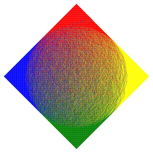
Figure 1: Uniformly random domino tilings of Aztec diamond with a perturbation of weight 10 along the up-right edge. See Example 7 for details.

Examples in a discrete setup

In Examples 6 and 7 we provide new results about two specific discrete systems. We formulate the results briefly here in the introduction; see the main part of the paper for more details.

Let $\gamma>1$ and $\alpha>0$ be fixed real numbers. Let $\varrho_{dBBP}(N)$ be a probability measure on $\hat{U}(N)$ corresponding to the Schur generating function

$$S_{\varrho_{dBBP}(N)}^{U(N)}(u_{1},\ldots,u_{N}):=\prod_{i=1}^{N}\exp\left(\gamma N(u_{i}-1)\right)\frac{1}{1-\alpha(u_{i}-1)}.$$

It is known that such a probability measure exists, since the expression above comes from an extreme character of the infinite-dimensional unitary group (see Section 6). For any $k\in\mathbb{N}$, in Example 6 we establish the following asymptotic expansion

$$\frac{1}{N}\sum_{\lambda\in\hat{U}(N)}\varrho_{dBBP}(N)[\lambda]\sum_{i=1}^{N}\left(\frac{\lambda_{i}+N-i}{N}\right)^{k}=\mathbf{m}_{k;dBBP}+\frac{1}{N}\mathbf{m}^{\prime}_{k;dBBP}+o\left(\frac{1}{N}\right),\qquad N\to\infty,$$ (15)

where

$$\mathbf{m}_{k;dBBP}=\int_{\mathbb{R}}t^{k}d\mu_{dBBP},\qquad\mathbf{m}^{\prime}_{k;dBBP}=\int_{\mathbb{R}}t^{k}d\mu^{\prime}_{dBBP},$$

while a probability measure $\mu_{dBBP}$ and a signed measure $\mu^{\prime}_{dBBP}$ are given by

$$d\mu_{dBBP}=\frac{1}{\pi}\mathbf{1}_{t\in[\gamma+1-2\sqrt{\gamma},\gamma+1+2\sqrt{\gamma}]}\arccos\left(\frac{t-1+\gamma}{2\sqrt{\gamma t}}\right)dt,$$

$$d\mu^{\prime}_{dBBP}=\delta\left(\alpha+1+\gamma+\frac{\gamma}{\alpha}\right)\mathbf{1}_{\alpha>\sqrt{\gamma}}+\frac{1}{2}\delta\left(\alpha+1+\gamma+\frac{\gamma}{\alpha}\right)\mathbf{1}_{\alpha=\sqrt{\gamma}}\\ +\left(\frac{\alpha(t-2\alpha-\gamma-1)}{\gamma+\alpha^{2}+\alpha\gamma+\alpha-\alpha t}-\frac{t+1-\gamma}{2t}\right)\frac{1}{2\pi\sqrt{(\gamma+1+2\sqrt{\gamma}-t)(t-\gamma-1+2\sqrt{\gamma})}}\mathbf{1}_{t\in[(\sqrt{\gamma}-1)^{2};(\sqrt{\gamma}+1)^{2}]}dt.$$ (16)

The new result is the second term in the right-hand side of (15), given by an explicit formula (16); the first term is essentially known from [Bia2], see also [BBO]. An important feature of the result is the presence of delta measures in (16) – in fact, this can be viewed as a discrete analog of a well-known Baik-Ben Arous-Peche phase transition for random matrices. It appears in the following setup. Consider the sum of a GUE matrix and a rank-one matrix. Then, depending on the value of a parameter in the rank-one matrix, the outlier in the empirical measure might or might not appear (we recall the exact details in Example 5).

The probability measure $\varrho_{dBBP}$ can be thought of in a similar way – the $\gamma N$ parameter comes from the one-sided Plancherel character, which is a discrete version of a GUE matrix, while $\alpha$ parameter plays the role of a rank-one matrix. The product of these two characters corresponds to the tensor product of representations, which is a discrete analog of the summation of matrices. We see that depending on whether $\alpha>\sqrt{\gamma}$, the outlier does or does not appear in the model.

Another example that we consider is a deformation of a model of uniformly random domino tilings of the Aztec diamond. It is well-known (we refer to [BK, Section 2] for a detailed discussion) that the domino tilings are in bijection with sequences of signatures $(\lambda^{1},\mu^{1},\dots,\lambda^{M})$ satisfying the following interlacing conditions:

$$\varnothing\prec\lambda^{1}\succ_{v}\mu^{1}\prec\lambda^{2}\succ_{v}\mu^{2}\prec\dots\prec\lambda^{M}\succ_{v}\varnothing.$$

Therefore, the uniform measure on the domino tilings of the Aztec diamond is equivalent to choosing uniformly at random such a sequence; also, geometric properties of the tilings are encoded by the signatures. Let $A>1$ be a fixed real number. We consider a deformation of the model by attaching the probability $ZA^{|\lambda^{M}|}$ to each sequence, where $Z$ is the normalizing factor, and $|\lambda^{M}|$ is the sum of all coordinates of $\lambda^{M}$. Geometrically, this means that we consider dominoes adjacent to the up-right edge of the Aztec diamond (drawn as in Figure 1), count how many of them are horizontal (they are colored in yellow in Figure 1), and the probability of a domino tiling is proportional to $A$ to the power of this amount.

Let $\varrho_{A}(N)$ be a distribution of $\lambda^{N}$ under this measure, where $1\leq N\leq M$. We assume that $N=\alpha M$, where $\frac{1}{2}<\alpha<1$ is a fixed real number. For any $k\in\mathbb{N}$, we obtain in Example 7 the asymptotic expansion

$$\frac{1}{N}\sum_{\lambda\in\hat{U}(N)}\varrho_{A}(N)[\lambda]\sum_{i=1}^{N}\left(\frac{\lambda_{i}+N-i}{N}\right)^{k}=\mathbf{m}_{k;A}+\frac{1}{N}\mathbf{m}^{\prime}_{k;A}+o\left(\frac{1}{N}\right),\qquad N\to\infty,$$ (17)

where

$$\mathbf{m}_{k;A}=\int_{\mathbb{R}}t^{k}d\mu_{A},\qquad\mathbf{m}^{\prime}_{k;A}=\int_{\mathbb{R}}t^{k}d\mu^{\prime}_{A},$$

and

$$d\mu_{A}=\mathbf{1}_{(1-2\alpha t)^{2}\leq 1-(1-2\alpha)^{2}}\frac{1}{\pi}\arccos\left(\frac{1-2\alpha}{\sqrt{1-(2\alpha t-1)^{2}}}\right)dt+\mathbf{1}_{1\geq(1-2\alpha t)^{2}>1-(1-2\alpha)^{2}}dt,$$ (18)

$$d\mu^{\prime}_{A}=-\mathbf{1}_{\alpha>\frac{(A+1)^{2}}{2(A^{2}+1)}}\delta\left(\frac{-1+2\alpha A-A}{\alpha(A^{2}-1)}\right)-\frac{1}{2}\mathbf{1}_{\alpha=\frac{(A+1)^{2}}{2(A^{2}+1)}}\delta\left(\frac{-1+2\alpha A-A}{\alpha(A^{2}-1)}\right)\\ +\left(\alpha+\frac{-2\alpha+1}{4t}-\frac{\alpha(2\alpha-1)}{4(\alpha t-1)}+\frac{\alpha(2A^{2}\alpha-A^{2}-2A+2\alpha-1)}{2(-\alpha t+A^{2}\alpha t-2\alpha A+1+A)}\right)\frac{\mathbf{1}_{1-(2\alpha-1)^{2}-(2\alpha t-1)^{2}>0}}{\pi\sqrt{1-(2\alpha-1)^{2}-(2\alpha t-1)^{2}}}dt.$$ (19)

The new result is the second term in the right-hand side of (17), given by an explicit formula (19). The first term is given by the arctic circle theorem, see [JPS], [CKP], [KO], [J].

Let us explain how this formula corresponds to geometric properties of a tiling. Since we scale in Theorem 3 by $N$, while geometrically we scale by $M$ in both directions (so that the Aztec diamond remains a square after the rescaling), we need to introduce variable $\tilde{y}=\alpha y$ for a horizontal direction. In coordinates $(\tilde{y},\alpha)$ the last summand of the correction measure (19) provides the density of the correction inside the arctic circle $1-(2\alpha-1)^{2}-(2\tilde{y}-1)^{2}=0$. Next, we see that the outlier is present if and only if $\alpha>\frac{(A+1)^{2}}{2(A^{2}+1)}$ at point $\tilde{y}=\frac{-1+2\alpha A-A}{(A^{2}-1)}$. Therefore, the outliers form a segment on a line $\frac{1-A^{2}}{2A}\alpha+\tilde{y}=\frac{A+1}{2A}$, which is tangent to the arctic circle and intersects with it at the point $\left(\frac{1}{A^{2}+1},\frac{(A+1)^{2}}{2(A^{2}+1)}\right)$. Thus, the result matches the effect visible in Figure 1.

It is interesting to note that the perturbation described above is similar to the one considered in the Tangent Method, see [CS], [A], [DG1], [DG2], [KDR], [R]. In this method, one fixes positions of dominoes along the up-right edge of the Aztec diamond and considers uniformly random domino tilings of the remaining domain. As shown by the computation above, our introduction of a parameter $A$ leads to the same asymptotic behavior of outliers and the dominoes along the up-right edge as prescribed by the Tangent Method. However, in principle these are two distinct perturbations; for example, it is not obvious whether the correction measures inside the arctic circle should also coincide for these two perturbations.

Higher order freeness

Given the connection of the Harish-Chandra transform and infinitesimal freeness from Theorem 2, it is natural to attempt to access further information about the averaged empirical measure. Our further results allow to extract next terms of its asymptotic expansion from the information about the Harish-Chandra transform. We establish two results in this direction for two slightly different asymptotic regimes.

The main result of Section 7 is the following.

Theorem 4

(Theorem 16) Let $A$ be a random Hermitian matrix of size $N$ and assume that for every finite $r$ one has

$$\lim_{N\rightarrow\infty}N^{2}\left(\frac{1}{N}\log\mathbb{E}[H\text{}C(x_{1},\ldots,x_{r},0^{N-r};\lambda_{1}(A),\ldots,\lambda_{N}(A))]-\sum_{i=1}^{r}\Psi(x_{i})-\frac{1}{N}\sum_{i=1}^{r}\Phi(x_{i})\right)=\sum_{i=1}^{r}\mathrm{T}(x_{i}),$$ (20)

where $\Psi,\Phi,\mathrm{T}$ are smooth functions in a complex neighborhood of $0$ and the above convergence is uniform in a complex neighborhood of $0^{r}$. Then the $1/N^{2}$ correction of the average empirical distribution of $N^{-1}A$ is given by

$$\lim_{N\rightarrow\infty}N^{2}\left(\frac{1}{N^{k+1}}\mathbb{E}[\operatorname{Tr}(A^{k})]-\boldsymbol{\mu}_{k}-\frac{1}{N}\boldsymbol{\mu}^{\prime}_{k}\right)=\boldsymbol{\mu}^{\prime\prime}_{k}+\boldsymbol{\nu}^{\prime\prime}_{k},$$

where $(\boldsymbol{\mu}_{k})_{k\in\mathbb{N}},(\boldsymbol{\mu}^{\prime}_{k})_{k\in\mathbb{N}}$ are given by (7),(8) respectively. The sequences $(\boldsymbol{\mu}^{\prime\prime}_{k})_{k\in\mathbb{N}},(\boldsymbol{\nu}^{\prime\prime}_{k})_{k\in\mathbb{N}}$ are given by

$$\boldsymbol{\mu}^{\prime\prime}_{k}=\sum_{m=0}^{k-1}\frac{k!}{m!(m+1)!(k-m-1)!}\left.\frac{\mathrm{d}^{m}}{\mathrm{d}x^{m}}((\Psi^{\prime}(x))^{k-m-1}\mathrm{T}^{\prime}(x))\right|_{x=0}$$

$$\text{{\hskip 100.00015pt}}+\frac{1}{2}\sum_{m=0}^{k-2}\frac{k!}{m!(m+1)!(k-m-2)!}\left.\frac{\mathrm{d}^{m}}{\mathrm{d}x^{m}}((\Psi^{\prime}(x))^{k-m-2}(\Phi^{\prime}(x))^{2})\right|_{x=0}$$ (21)

and

$$\boldsymbol{\nu}^{\prime\prime}_{k}=\frac{1}{24}\sum_{m=0}^{k-3}\frac{k!}{m!(m+1)!(k-m-3)!}\left.\frac{\mathrm{d}^{m}}{\mathrm{d}x^{m}}((\Psi^{\prime}(x))^{k-m-3}\Psi^{\prime\prime\prime}(x))\right|_{x=0}$$

$$\text{{\hskip 40.00006pt}}+\frac{1}{12}\sum_{m=0}^{k-3}\frac{k!}{m!(m+2)!(k-m-3)!}\left.\frac{\mathrm{d}^{m}}{\mathrm{d}x^{m}}((\Psi^{\prime}(x))^{k-m-3}\Psi^{\prime\prime\prime}(x))\right|_{x=0}$$

$$\text{{\hskip 100.00015pt}}+\frac{1}{12}\sum_{m=0}^{k-4}\frac{k!}{m!(m+2)!(k-m-4)!}\left.\frac{\mathrm{d}^{m}}{\mathrm{d}x^{m}}((\Psi^{\prime}(x))^{k-m-4}(\Psi^{\prime\prime}(x))^{2})\right|_{x=0}.$$ (22)

As visible from the result, new effects appear in the analysis of the third asymptotic term. Despite the fact that condition (20) is similar to condition (5), the structure of the answer is more complicated than in Theorem 2. As explained in Lemma 7, the term (21) comes from the second order infinitesimal freeness. However, the term (22) is more specific to the scaling under consideration, and does not have an analog for the first order correction. It would be interesting to establish a connection of explicit formulas (21), (22) with the description for higher order free cumulants given in [BCGLS]; we do not address this question.

The main result of Section 8 is the following.

Theorem 5

(Theorem 17) Let $n$ be a fixed integer. Let $A$ be a random Hermitian matrix of size $N$ and assume that for every finite $r$ one has

$$\lim_{N\rightarrow\infty}N^{n\varepsilon}\left(\frac{1}{N}\log\mathbb{E}[H\text{}C(x_{1},\ldots,x_{r},0^{N-r};\lambda_{1}(A),\ldots,\lambda_{n}(A))]-\sum_{j=0}^{n-1}\sum_{i=0}^{r}\frac{1}{N^{j\varepsilon}}\Psi_{j}(x_{i})\right)=\sum_{i=1}^{r}\Psi_{n}(x_{i}),$$ (23)

where $\Psi_{0},\ldots,\Psi_{n}$ are smooth functions in a complex neighborhood of $0$, the above convergence is uniform in a complex neighborhood of $0^{r}$, and $0<\varepsilon<n^{-1}$. Then the $1/N^{n\varepsilon}$ correction of the average empirical distribution of $N^{-1}A$ is given by

$$\lim_{N\rightarrow\infty}N^{n\varepsilon}\left(\frac{1}{N^{k+1}}\mathbb{E}[\operatorname{Tr}(A^{k})]-\sum_{j=0}^{n-1}\frac{1}{N^{j\varepsilon}}\boldsymbol{\mu}^{(j)}_{k}\right)=\boldsymbol{\mu}_{k}^{(n)},$$ (24)

where for every $j\in\{0,\ldots,n\}$

$$\boldsymbol{\mu}^{(j)}_{k}:=\sum_{b_{1}+2b_{2}+\cdots+j\text{}b_{j}=j}\sum_{m=0}^{k-b_{1}-\cdots-b_{j}}\frac{k!}{m!(m+1)!(k-m-b_{1}-\cdots-b_{j})!b_{1}!\ldots b_{j}!}\text{{\hskip 80.00012pt}}$$

$$\text{{\hskip 140.00021pt}}\times\left.\frac{\mathrm{d}^{m}}{\mathrm{d}x^{m}}((\Psi^{\prime}_{0}(x))^{k-m-b_{1}-\cdots-b_{j}}(\Psi^{\prime}_{1}(x))^{b_{1}}\ldots(\Psi^{\prime}_{j}(x))^{b_{j}})\right|_{x=0}.$$ (25)

The introduction of parameter $\epsilon$ and the limit regime (23) simplify the structure of the answer. We connect formula (25) with higher order infinitesimal freeness introduced in [F]; nevertheless, the explicit formula (25) seems to be new. We would like to emphasize that the main feature of Theorem 5, as well as other key results of the current paper, is that condition (23) is of general nature — we do not assume the explicit form of the Harish-Chandra transform, only the asymptotic information about it.

In Sections 7 and 8 we also provide several examples with detailed calculations. In particular, in Example 11 we study a version of a higher order BBP phase transition.

Acknowledgments

We are grateful to Alexei Borodin,Vadim Gorin and Leonid Petrov for valuable comments. We used the code by Sunil Chhita in order to produce Figure 1. Both authors were partially supported by the European Research Council (ERC), Grant Agreement No. 101041499.

2 Preliminaries

Voiculescu’s free probability theory ([V1], [V2], [NS]) provides a natural framework to study families of random matrices as their size goes to infinity. The reason is that many classes of large random matrices behave like freely independent random variables. A typical situation where this phenomenon occurs is the summation of random matrices. For example, consider the case of two independent $N\times N$ Hermitian random matrices $A_{1},A_{2}$ with deterministic eigenvalues $\{\lambda_{1}(A_{1})\leq\cdots\leq\lambda_{N}(A_{1})\}$, $\{\lambda_{1}(A_{2})\leq\cdots\leq\lambda_{N}(A_{2})\}$ and eigenvectors chosen uniformly (=Haar distributed) at random. Under convergence assumptions for the empirical distributions $N^{-1}\sum_{i=1}^{N}\delta\left(\lambda_{i}(A_{j})\right)$, $j=1,2$, one can deduce the convergence for the (random) empirical distribution of $A_{1}+A_{2}$. The limit of $A_{1}+A_{2}$ (meaning the limit of its empirical distribution) can be uniquely determined in terms of the limits of $A_{1},A_{2}$ by quantities called free cumulants. The summation $A_{1}+A_{2}$ translates into the summation of the free cumulants that correspond to the limits of $A_{1}$ and $A_{2}$.

Infinitesimal free probability theory goes a step further and studies not only the limit of $A_{1}+A_{2}$ but also its $1/N$ correction, that is, the second leading term in the asymptotic expansion of the expectation of observables of $A_{1}+A_{2}$. This question attracted additional attention due to its connection with finite-rank perturbations of random matrices [BBP], [BS], [Sh]. In this context, let $A_{3}$ be a $N\times N$ finite-rank (i.e., its rank does not grow with $N$), Hermitian and deterministic matrix. Its empirical distribution converges to $\delta\left(0\right)$ and its $1/N$ correction is given by

$$\sum_{\lambda\in\text{ non-zero eigenvalues of }A_{3}}(\delta\left(\lambda\right)-\delta\left(0\right)).$$

Assuming the convergence for the empirical measure of $A_{1}$, the leading order limits of $A_{1}$ and $A_{1}+A_{3}$ are equal to each other. However, the existence of $A_{3}$ in $A_{1}+A_{3}$ affects the $1/N$ correction. This can be obtained from the fact that free independence of $A_{1},A_{3}$ does not only give a rule for the limit of $A_{1}+A_{3}$, but also for its $1/N$ correction. The description of this rule can be presented with the use of quantities that generalize the notion of free cumulants; they are known as infinitesimal free cumulants. They were introduced and studied in [BS], [FN].

In the current paper we also study arbitrary order corrections to the limit of the empirical distribution of certain random matrix models. We make explicit calculations for higher order corrections on different scales. Specifically, we compute the $n$-th order correction on the scale $1/N^{\varepsilon}$, with $0<\varepsilon\leq 1$, for a $N\times N$ Hermitian random matrix $A$, by obtaining an asymptotic expansion

$$\frac{1}{N}\mathbb{E}[\operatorname{Tr}(A^{k})]=\sum_{i=0}^{n}M_{i,k,N}\frac{1}{N^{i\varepsilon}}+\omicron(N^{-n\varepsilon})\text{, \quad for every }k\in\mathbb{N},$$ (26)

where $(M_{i,k,N})_{N\in\mathbb{N}}$ are convergent sequences of real numbers. We prove the existence of an expansion of the form (26) under general assumptions on the asymptotic behavior of Harish-Chandra transforms, see Section 1.

Let us now turn to formal definitions. We begin by recalling the basic notions of non-commutative/free probability and some of its basic tools.

Definition 1 (Non-commutative probability)

A non-commutative probability space consists of a unital algebra $\mathcal{A}$ over $\mathbb{C}$ and a linear functional $\varphi:\mathcal{A}\rightarrow\mathbb{C}$, such that $\varphi(1_{\mathcal{A}})=1$. The elements of $\mathcal{A}$ are called non-commutative random variables. The non-commutative distribution of $a\in\mathcal{A}$ is the linear functional $\mu_{a}:\mathbb{C}\langle\mathbf{x}\rangle\rightarrow\mathbb{C}$, defined by

$$\mu_{a}(P):=\varphi(P(a))\text{, \quad for every ploynomial }P\in\mathbb{C}\langle\mathbf{x}\rangle.$$

For $(a_{1},\ldots,a_{n})\in\mathcal{A}^{n}$ the values $\varphi(a_{1}\ldots a_{n})$ are called moments.

The framework described in Definition 1 can be seen as a generalization of the classical probabilistic setting. For this, one considers the algebra of (integrable) random variables as the fundamental object, instead of a probability space $(\Omega,\mathcal{F},\mathbb{P})$. In that case, the expectation $\mathbb{E}$ will play the role of the linear functional. In the current paper, we are interested in the following non-commutative probability space.

Example 1

Let $\mathrm{M}_{N}(L^{\infty-}(\Omega,\mathcal{F},\mathbb{P}))$ be the algebra of $N\times N$ matrices, whose entries are complex-valued random variables such that all their moments exist. The tuple $(\mathrm{M}_{N}(L^{\infty-}(\Omega,\mathcal{F},\mathbb{P})),N^{-1}\mathbb{E}[\operatorname{Tr}(\cdot)])$ is a non-commutative probability space.

Free probability deals with the notion of free independence in non-commutative spaces. A combinatorial description of free independence was developed in [Sp]; it is based on cumulant functionals, known as free cumulants. A partition $\pi$ of $\{1,\ldots,k\}$ is called non-crossing if for all blocks $V=\{v_{1}<\cdots<v_{n}\}$ and $W=\{w_{1}<\cdots<w_{m}\}$ we have $v_{r}<w_{1}<v_{r+1}$ for some $r=1,\ldots,n-1$ if and only if $v_{r}<w_{m}<v_{r+1}$. We denote the set of non-crossing partitions of $\{1,\ldots,k\}$ by $\operatorname{NC}(k)$. Non-crossing partitions can be visualized in the following way: If we connect with ”bridges” the points of $\{1,\ldots,k\}$ that belong to the same block of $\pi$, then $\pi$ is non-crossing if and only if these bridges do not cross.

Definition 2 (Free cumulants)

Let $(\mathcal{A},\varphi)$ be a non-commutative probability space. The multilinear functionals $(\kappa_{n}:\mathcal{A}^{n}\rightarrow\mathbb{C})_{n\in\mathbb{N}}$ uniquely determined by the relation

$$\varphi(a_{1}\ldots a_{k})=\sum_{\pi\in\operatorname{NC}(k)}\prod_{\{i_{1}<\cdots<i_{s}\}\in\pi}\kappa_{s}(a_{i_{1}},\ldots,a_{i_{s}})\text{, \quad for every $k\in\mathbb{N}$ and }(a_{1},\ldots,a_{k})\in\mathcal{A}^{k},$$ (27)

are called free cumulants of $(\mathcal{A},\varphi)$.

The relation between free independence and free cumulants comes from the fact that two non-commutative random variables are freely independent if and only if certain free cumulants vanish (see, e.g., [NS]). Therefore, for freely independent $a,b\in(\mathcal{A},\varphi)$, one has

$$\kappa_{n}(a+b,\ldots,a+b)=\kappa_{n}(a,\ldots,a)+\kappa_{n}(b,\ldots,b)\text{, \quad for every }n\in\mathbb{N}.$$

The main connection between random matrices and free probability comes from the fact that free probability provides a natural framework for many classes of random matrices as their size goes to infinity, see, e.g., [NS], [AGZ]. In particular, it describes large Hermitian random matrices with fixed spectrum and eigenvectors chosen uniformly at random. Two independent such matrices $A_{1},A_{2}$, under asymptotic conditions for their spectra, become asymptotically freely independent. In more detail, one has the following result.

Theorem 6 (Voiculescu)

Let $A_{1}=U_{1}\text{}\operatorname{diag}(a^{(1)}_{1},\ldots,a^{(1)}_{N})U_{1}^{\ast}$ and $A_{2}=U_{2}\operatorname{diag}(a^{(2)}_{1},\ldots,a^{(2)}_{N})U_{2}^{\ast}$ be Hermitian random matrices of size $N$, where $U_{1},U_{2}$ are chosen independently at random with respect to the Haar measure on the unitary group $U(N)$ and $\{a_{i}^{(j)}\}_{i,j}$ are fixed and such that for $j=1,2$ the empirical distribution of $A_{j}$ converges weakly to a probability measure $\boldsymbol{\mu}_{j}$. Then the random empirical distribution of $A_{1}+A_{2}$ converges weakly, in probability to a deterministic probability measure $\boldsymbol{\mu}_{1}\boxplus\boldsymbol{\mu}_{2}$.

The probability measure $\boldsymbol{\mu}_{1}\boxplus\boldsymbol{\mu}_{2}$ is known as the free convolution of $\boldsymbol{\mu}_{1}$ and $\boldsymbol{\mu}_{2}$. It can be described via corresponding free cumulant sequences $(\kappa_{n}(\boldsymbol{\mu}_{1}))_{n\in\mathbb{N}},(\kappa_{n}(\boldsymbol{\mu}_{2}))_{n\in\mathbb{N}}$, which are uniquely determined by the relations

$$\int_{\mathbb{R}}t^{k}\boldsymbol{\mu}_{j}(d\text{}t)=\sum_{\pi\in\operatorname{NC}(k)}\prod_{V\in\pi}\kappa_{|V|}(\boldsymbol{\mu}_{j})\text{, \quad for every }k\in\mathbb{N}\text{ and }j=1,2.$$

Namely, one has:

$$\kappa_{n}(\boldsymbol{\mu}_{1}\boxplus\boldsymbol{\mu}_{2})=\kappa_{n}(\boldsymbol{\mu}_{1})+\kappa_{n}(\boldsymbol{\mu}_{2})\text{, \quad for every }n\in\mathbb{N}.$$

In the next sections we are interested in the corrections to this limit. We want to understand these corrections through quantities that are generalizations of free cumulants and encode the notion of higher order infinitesimal freeness. The abstract setting is the following.

Definition 3

An infinitesimal non-commutative probability space of order $\nu$ is a $(\nu+1)$-tuple $(\mathcal{A},\varphi^{(0)},\ldots,\varphi^{(\nu)})$, where $(\mathcal{A},\varphi^{(0)})$ is a non-commutative probability space and $\varphi^{(i)}:\mathcal{A}\rightarrow\mathbb{C}$ are linear functionals such that $\varphi^{(i)}(1_{\mathcal{A}})=0$, for every $i=1,\ldots,\nu$. The infinitesimal non-commutative distribution of order $n$ of $a\in\mathcal{A}$ is the $(n+1)$-tuple $(\mu_{a}^{(i)}:\mathbb{C}\langle\mathbf{x}\rangle\rightarrow\mathbb{C})_{i=0}^{n}$ of linear functionals, defined by

$$\mu_{a}^{(i)}(P)=\varphi^{(i)}(P(a))\text{, \quad for every }P\in\mathbb{C}\langle\mathbf{x}\rangle\text{ and }i=0,\ldots,\nu.$$

We are interested in infinitesimal non-commutative probability spaces $(\mathcal{A},\varphi^{(0)},\ldots,\varphi^{(\nu)})$ that emerge as the infinitesimal limit of a family $(\mathcal{A},\varphi_{t})_{t\in\mathbb{R}}$ of non-commutative probability spaces. This means that for $a\in\mathcal{A}$, $\varphi^{(0)}(a),\ldots,\varphi^{(\nu)}(a)$ are uniquely determined by

$$\frac{\varphi^{(\nu)}(a)}{\nu!}=\lim_{t\rightarrow 0}\frac{1}{t^{\nu}}\left(\varphi_{t}(a)-\sum_{i=0}^{\nu-1}\varphi^{(i)}(a)\frac{t^{i}}{i!}\right).$$ (28)

Thus, we have $\lim_{t\rightarrow 0}\varphi_{t}(a)=\varphi^{(0)}(a)$, for every $a\in\mathcal{A}$ and for $i=1,\ldots,\nu$ the “derivative” $\varphi^{(i)}$ plays the role of the $i$-th order correction to the above limit. For $\nu=1$ this is the framework of the infinitesimal free probability, introduced in [BS]. They introduced a notion of infinitesimal freeness which provides a rule for computing moments of random variables in $(\mathcal{A},\varphi^{(0)},\varphi^{(1)})$, assuming that they are freely independent in $(\mathcal{A},\varphi_{t})$ for every $t\in\mathbb{R}$. In the same direction, the notion of infinitesimal free cumulants was introduced in [FN]. The moments of random variables in $(\mathcal{A},\varphi^{(0)},\varphi^{(1)})$ can be written in terms of these cumulants in a similar to (27) way. In more detail, the infinitesimal free cumulants $(\kappa^{(0)}_{n},\kappa^{(1)}_{n}:\mathcal{A}^{n}\rightarrow\mathbb{C})_{n\in\mathbb{N}}$ are defined in the following way: $(\kappa_{n}^{(0)})_{n\in\mathbb{N}}$ are the free cumulants of $(\mathcal{A},\varphi^{(0)})$ and $(\kappa_{n}^{(1)})_{n\in\mathbb{N}}$ are uniquely determined by

$$\varphi^{(1)}(a_{1}\ldots a_{k})=\sum_{\pi\in\operatorname{NC}(k)}\sum_{V=\{i_{1}<\cdots<i_{s}\}\in\pi}\kappa_{s}^{(1)}(a_{i_{1}},\ldots,a_{i_{s}})\prod_{\underset{W\neq V}{W=\{j_{1}<\cdots<j_{l}\}\in\pi}}\kappa_{l}^{(0)}(a_{j_{1}},\ldots,a_{j_{l}}),$$ (29)

for every $k\in\mathbb{N}$ and $(a_{1},\ldots,a_{k})\in\mathcal{A}^{k}$. Formula (29) can be thought of as that there is an (informal) differentiation procedure to pass from $\varphi^{(0)}$ to $\varphi^{(1)}$, starting from the moment-cumulant relations (27). Namely, if $\kappa_{n}^{(1)}(a_{1},\ldots,a_{n})$ is considered as the derivative of $\kappa_{n}^{(0)}(a_{1},\ldots,a_{n})$ and $\varphi^{(1)}(a_{1}\ldots a_{n})$ as the derivative of $\varphi^{(0)}(a_{1}\ldots a_{n})$, applying derivatives in (27) and using Leibniz rule, we get (29). In a similar vein, the infinitesimal free cumulants $(\kappa_{n}^{(0)})_{n\in\mathbb{N}}$ and $(\kappa_{n}^{(1)})_{n\in\mathbb{N}}$ of $(\mathcal{A},\varphi^{(0)},\varphi^{(1)})$ satisfy the relations

$$\kappa_{n}^{(0)}(a_{1},\ldots,a_{n})=\lim_{t\rightarrow 0}\kappa_{n}^{(t)}(a_{1},\ldots,a_{n})\text{\quad and\quad}\kappa_{n}^{(1)}(a_{1},\ldots,a_{n})=\left.\frac{\mathrm{d}}{\mathrm{d}t}\kappa_{n}^{(t)}(a_{1},\ldots,a_{n})\right|_{t=0},$$

where $(\kappa_{n}^{(t)})_{n\in\mathbb{N}}$ are the free cumulants of $(\mathcal{A}{,}\varphi_{t})$.

Remark 1

Similarly with the free independence, the infinitesimal freeness can be characterized by infinitesimal free cumulants. Two random variables in $(\mathcal{A},\varphi^{(0)},\varphi^{(1)})$ are infinitesimally free if and only if certain infinitesimal free cumulants vanish (see [FN]). As a corollary, infinitesimally free variables $a,b\in(\mathcal{A},\varphi^{(0)},\varphi^{(1)})$ satisfy

$$\kappa_{n}^{(i)}(a+b,\ldots,a+b)=\kappa_{n}^{(i)}(a,\ldots,a)+\kappa_{n}^{(i)}(b,\ldots,b),\text{\quad for every }n\in\mathbb{N}\text{ and }i=0,1.$$

Motivated by the construction of infinitesimal free cumulants for $(\mathcal{A},\varphi^{(0)},\varphi^{(1)})$, one can extend the notion of infinitesimal free cumulants for $(\mathcal{A},\varphi^{(0)},\varphi^{(1)},\ldots,\varphi^{(\nu)})$. Since $\varphi^{(i)}$ plays the role of the $i$-th derivative of $\varphi^{(0)}$, the infinitesimal free cumulants of higher order $\kappa_{n}^{(i)}$ can be seen as the $i$-th derivative of $\kappa_{n}^{(0)}$. In that way, starting from the relation (27) between $\varphi^{(0)}$, $(\kappa_{n}^{(0)})_{n\in\mathbb{N}}$ and differentiating step by step, we can determine $(\kappa_{n}^{(i)})_{n\in\mathbb{N}}$ with the use of $\varphi^{(i)},(\kappa_{n}^{(0)})_{n\in\mathbb{N}},\ldots,(\kappa_{n}^{(i-1)})_{n\in\mathbb{N}}$. In order to write the exact formula that describes this relation, we introduce some notation.

Notation 1

Let $(\psi_{n}:\mathcal{A}^{n}\rightarrow\mathbb{C})_{n\in\mathbb{N}}$ be a family of multilinear functionals and $\pi$ be a partition of $\{1,\ldots,k\}$. Given a block $V=\{i_{1}<\cdots<i_{s}\}$ of $\pi$ and $(a_{1},\ldots,a_{k})\in\mathcal{A}^{k}$, we define

$$\psi_{|V|}(a_{1},\ldots,a_{k}|V):=\psi_{s}(a_{i_{1}},\ldots,a_{i_{s}}).$$

Definition 4

Let $(\mathcal{A},\varphi^{(0)},\varphi^{(1)},\ldots,\varphi^{(\nu)})$ be an infinitesimal non-commutative probability space of order $\nu$. The infinitesimal free cumulants of order $\nu$ are multilinear maps $(\kappa_{n}^{(0)},\ldots,\kappa_{n}^{(\nu)}:\mathcal{A}^{n}\rightarrow\mathbb{C})$ uniquely determined by the following relation: For every $k\in\mathbb{N}$, $i=0,\ldots,\nu$ and $(a_{1},\ldots,a_{k})\in\mathcal{A}^{k}$,

$$\varphi^{(i)}(a_{1}\ldots a_{k})=\sum_{\pi=\{V_{1},\ldots,V_{p}\}\in\operatorname{NC}(k)}\sum_{\lambda_{1}+\cdots+\lambda_{p}=i}\frac{i!}{\lambda_{1}!\ldots\lambda_{p}!}\prod_{i=1}^{p}\kappa_{|V_{i}|}^{(\lambda_{i})}(a_{1},\ldots,a_{k}|V_{i}).$$ (30)

Note that Definition 4 is consistent with our description of the infinitesimal free cumulants of higher order since the latter sum in the right hand side of (30) plays the role of the $i$-th derivative of $\prod_{V\in\pi}\kappa^{(0)}_{|V|}(a_{1},\ldots,a_{k}|V)$. Formula (30) for the infinitesimal free cumulants of higher order was introduced in [F]. Analogously to the connection of the (infinitesimal) freeness (of order $1$) and (infinitesimal) free cumulants (of order $1$), in [F] the notion of higher order freeness is introduced as a rule for vanishing certain higher order infinitesimal free cumulants. This is consistent with the cases $\nu=0,1$, and for two infinitesimally free of order $\nu$ random variables $a,b\in(\mathcal{A},\varphi^{(0)},\ldots,\varphi^{(\nu)})$ we have

$$\kappa_{n}^{(i)}(a+b,\ldots,a+b)=\kappa_{n}^{(i)}(a,\ldots,a)+\kappa_{n}^{(i)}(b,\ldots,b)\text{, \quad for every }n\in\mathbb{N}\text{ and }i=0,\ldots,\nu.$$

In the present paper, our interest is in infinitesimal non-commutative probability spaces of higher order that emerge as the infinitesimal limit of the non-commutative distribution of random matrix models. In more detail, given a Hermitian random matrix $A$ of size $N$, the linear functional that will play the role of $\varphi_{t}$ is

$$P\in\mathbb{C}\langle\mathbf{x}\rangle\mapsto\frac{1}{N}\mathbb{E}[\operatorname{Tr}\text{}P(A)],$$

where “$t=\frac{1}{N}$”. In this setting, in order to guarantee the existence of the infinitesimal limit of the form (28), we will focus on particular random matrix models. The simplest example is a GUE matrix, i.e. a Hermitian random matrix $A=(a_{i,j})_{i,j=1}^{N}$ such that $(a_{i,j})_{i\leq j}$ are independent centered complex Gaussian variables, with independent real and imaginary parts and covariances $\mathbb{E}[a_{i,j}a_{k,l}]=N^{-1}\delta_{i,l}\delta_{j,k}$, for every $1\leq i,j,k,l\leq N$. It is well known (see, e.g., [AGZ]) that for such a matrix, for every $k\in\mathbb{N}$ one has an asymptotic expansion

$$\frac{1}{N}\mathbb{E}[\operatorname{Tr}(A^{k})]=\sum_{n\geq 0}\frac{1}{N^{2n}}M_{n,k},$$ (31)

where $M_{n,k}$ are real numbers that do not depend on $N$. Relation (31) is called the topological expansion because the numbers $M_{n,k}$ are related to the enumeration of maps.

In the following sections we study random matrix models that have expansions similar to (31). Let $A$ be a Hermitian random matrix of size $N$ with real eigenvalues $\lambda_{1}(A),\ldots,\lambda_{N}(A)$. Our approach for computing the moments of the probability measure $N^{-1}\mathbb{E}\left[\sum_{i=1}^{N}\delta\left(\lambda_{i}(A)\right)\right]$ is based on a differentiation procedure of the characteristic/moment generating function of $A$. This is analogous to the fact that via differentiating the characteristic/moment generating function of a random variable one can get its moments. Therefore, we focus on classes of random matrices whose characteristic function can be controlled to some extent.

One class of such matrices is formed by ergodic unitarily invariant matrices. In the current paper they will be the main source of our examples. Ergodic random matrices were classified and studied in [OV] (see also [P]). We recall that given a probability measure $\boldsymbol{M}$ on the space of all infinite Hermitian matrices $H$, its characteristic function is defined via

$$f_{\boldsymbol{M}}(A):=\int_{H}\exp(\mathrm{i}\operatorname{Tr}(A\text{}B))\boldsymbol{M}(d\text{}B)\text{, \quad for every }A\in H(\infty),$$

where $H(\infty)\subset H$ is the space of infinite Hermitian matrices with finitely many non-zero entries. Let $U(\infty)\subseteq H$ be the group of inifinite unitary matrices $U=(u_{i,j})$ such that $u_{i,j}=\delta_{i,j}$ when $i+j$ is large enough and $D(\infty)\subseteq H(\infty)$ be the subspace of diagonal matrices in $H(\infty)$. For a $U(\infty)$-invariant Borel probability measure $\boldsymbol{M}$, the value $f_{\boldsymbol{M}}(A)$ depends only from the spectrum of $A\in H(\infty)$, since any matrix in $H(\infty)$ can be diagonalized under the action of $U(\infty)$. Then the Multiplicativity Theorem (see, e.g., [OV, Theorem 2.1]) states that $\boldsymbol{M}$ is ergodic if and only if for every $k\in\mathbb{N}$ the symmetric function $(a_{1},\ldots,a_{k})\mapsto f_{\boldsymbol{M}}(\operatorname{diag}(a_{1},\ldots,a_{k},0,\ldots))$ is multiplicative, in the sense that there exists a one-variable function $F_{\boldsymbol{M}}$, such that

$$f_{\boldsymbol{M}}(\operatorname{diag}(a_{1},\ldots,a_{k},0,\ldots))=\prod_{i=1}^{k}F_{\boldsymbol{M}}(a_{i})\text{, \quad for every }k\in\mathbb{N}\text{ and }a_{1},\ldots,a_{k}\in\mathbb{R}.$$

The function $F_{\boldsymbol{M}}$ is determined by $F_{\boldsymbol{M}}(a)=f_{\boldsymbol{M}}(\operatorname{diag}(a,0,\ldots))$, for every $a\in\mathbb{R}$. Let $\mathcal{F}$ denote the class of all these functions $F_{\boldsymbol{M}}$. The description of $\mathcal{F}$ leads to the classification of the ergodic measures $\boldsymbol{M}$.

Theorem 7

([OV], [P]) The class $\mathcal{F}$ consists of all the functions $F_{\gamma_{1},\gamma_{2},x}$ of the form

$$F_{\gamma_{1},\gamma_{2},x}(a)=\exp\left(\mathrm{i}\gamma_{1}a-\frac{\gamma_{2}}{2}a^{2}\right)\prod_{n=1}^{\infty}\frac{\exp(-\mathrm{i}x_{n}a)}{1-\mathrm{i}x_{n}a},$$ (32)

where $(x_{n})\in\mathbb{N}$ is a sequence of real numbers such that $\sum_{n\geq 1}x_{n}^{2}<\infty$ and $\gamma_{1}\in\mathbb{R}$, $\gamma_{2}\geq 0$.

Let us recall that for two $N\times N$ Hermitian matrices $A,B$ with eigenvalues $\lambda_{1}(A)\leq\cdots\leq\lambda_{N}(A)$ and $\lambda_{1}(B)\leq\cdots\leq\lambda_{N}(B)$, the Harish-Chandra integral (also known as Itzykson-Zuber integral) is defined by

$$H\text{}C(\lambda_{1}(A),\ldots,\lambda_{N}(A);\lambda_{1}(B),\ldots,\lambda_{N}(B)):=\int_{U(N)}\exp(\operatorname{Tr}(A\text{}U\text{}B\text{}U^{\ast}))\boldsymbol{m}_{N}(d\text{}U),$$ (33)

where $\boldsymbol{m}_{N}$ denotes the Haar measure on the unitary group $U(N)$ (see [HC]). Note that the right hand side of (33) depends only on ${\{\lambda_{i}(A),\lambda_{i}(B)\}_{i=1}^{N}}$. The above integral can be computed explicitly and it is equal to

$$c_{N}\frac{\det(\exp(\lambda_{i}(A)\lambda_{j}(B)))_{i,j=1}^{N}}{\prod_{1\leq i<j\leq N}(\lambda_{i}(A)-\lambda_{j}(B))\prod_{1\leq i<j\leq N}(\lambda_{i}(B)-\lambda_{j}(B))},$$ (34)

where $c_{N}=\prod_{i=1}^{N-1}i!$.

3 Free probability scaling

In this section we essentially recall the proof of [BG, Theorem 5.1], see Theorem 8 below. We do certain technical improvements along the way, which will allow us to use this section as a reference point for the proofs in the rest of the paper. We also present it here in the language of random matrices and Harish-Chandra transform, rather than a somewhat more general setup of discrete particle systems and Schur functions of [BG, Theorem 5.1], which we address in Section 6 below.

For every $k\in\mathbb{N}$ let us introduce a differential operator acting on smooth functions $f$ of $N$ variables $x_{1},x_{2},\dots,x_{n}$:

$$\mathcal{D}_{k}(f):=\left(\prod_{i<j}(x_{i}-x_{j})\right)^{-1}\sum_{i=1}^{N}\partial_{i}^{k}\left(\prod_{i<j}(x_{i}-x_{j})\cdot f\right).$$ (35)

Proposition 1

For the function $f_{\underset{\lambda}{\rightarrow}}(x_{1},\ldots,x_{N}):=H\text{}C(x_{1},\ldots,x_{N};\lambda_{1},\ldots,\lambda_{N})$ we have

$$\mathcal{D}_{k}\left(f_{\underset{\lambda}{\rightarrow}}\right)(x_{1},\ldots,x_{N})=\sum_{i=1}^{N}\lambda_{i}^{k}f_{\underset{\lambda}{\rightarrow}}(x_{1},\ldots,x_{N}).$$ (36)

Proof.

By the relation (34) and the Leibniz rule we have

$$\mathcal{D}_{k}\left(f_{\underset{\lambda}{\rightarrow}}\right) = \left(\prod_{i<j}(x_{i}-x_{j})(\lambda_{i}-\lambda_{j})\right)^{-1}\sum_{\pi\in S_{N}}\operatorname{sgn}(\pi)\left(\sum_{i=1}^{N}\lambda_{\pi(i)}^{k}\right)\prod_{i=1}^{N}\exp(x_{i}\lambda_{\pi(i)})$$

$$= \left(\sum_{i=1}^{N}\lambda_{i}^{k}\right)\left(\prod_{i<j}(x_{i}-x_{j})(\lambda_{i}-\lambda_{j})\right)^{-1}\det(\exp(x_{i}\lambda_{j}))_{i,j=1}^{N}=\sum_{i=1}^{N}\lambda_{i}^{k}f_{\underset{\lambda}{\rightarrow}}.$$

∎

Before stating the main theorem of this section, we give several lemmas which help us to understand how the differential operator $\mathcal{D}_{k}$ acts on smooth functions.

Lemma 1

For a smooth function $f$ of $N$ variables we have

$$\mathcal{D}_{k}(f)=\sum_{m=0}^{k}\sum_{\underset{l_{i}\neq l_{j}\text{ for }i\neq j}{l_{0},\ldots,l_{m}=1}}^{N}\binom{k}{m}\frac{\partial_{l_{0}}^{k-m}f}{(x_{l_{0}}-x_{l_{1}})\ldots(x_{l_{0}}-x_{l_{m}})}.$$ (37)

Proof.

For $l\in\{1,\ldots,N\}$ and $k\in\mathbb{N}$, by Leibniz rule, we have

$$\partial_{l}^{k}\left(\prod_{i<j}(x_{i}-x_{j})\cdot f\right)=(-1)^{l-1}\sum_{k_{1}+\cdots+k_{N}=k}\frac{k!}{k_{1}!\ldots k_{N}!}\prod_{\underset{i\neq l}{i=1}}^{N}\partial_{l}^{k_{i}}(x_{l}-x_{i})\partial_{l}^{k_{l}}f,$$ (38)

where in the product in the left hand side we omit terms of $\prod_{i<j}(x_{i}-x_{j})$ that do not depend on $x_{l}$. Consider the case, where $k_{l}=k-m$ and $k_{l_{1}}=\cdots=k_{l_{m}}=1$, for some $l_{1},\ldots,l_{m}\in\{1,\ldots,N\}\backslash\{l\}$, with $l_{i}\neq l_{j}$, for all $i\neq j$. Then, if we divide the corresponding summand of the left hand side of (38) to $\prod_{i<j}(x_{i}-x_{j})$, we get

$$\frac{k!}{(k-m)!}\frac{\partial_{l}^{k-m}f}{(x_{l}-x_{l_{1}})\ldots(x_{l}-x_{l_{m}})}.$$

Considering all the different choices of variables to differentiate, we obtain that the left hand side of (38) divided by $\prod_{i<j}(x_{i}-x_{j})$ is equal to

$$\sum_{\underset{l_{i}\neq l_{j}\text{ for }i\neq j}{l_{1},\ldots,l_{m}\in\{1,\ldots,N\}\backslash\{l\}}}\binom{k}{m}\frac{\partial_{l}^{k-m}f}{(x_{l}-x_{l_{1}})\ldots(x_{l}-x_{l_{m}})},$$

where in the above sum the binomial coefficient appears because for a fixed $m$-tuple $(l_{1},\ldots,l_{m})$ the summand $\frac{k!}{(k-m)!}\frac{\partial_{l}^{k-m}f}{(x_{l}-x_{l_{1}})\ldots(x_{l}-x_{l_{m}})}$ appears $m!$ times. If we take the sum with respect to $l=1,\ldots,N$ and $m=1,\ldots,k$, we arrive at the claim. ∎

The next lemma is a standard result which will help us to evaluate the differential operator at zero, see e.g., [BG, Lemma 5.5].

Lemma 2

Let $n\geq 2$ and a function $f$ smooth in a neighborhood of $0$. Then

$$\lim_{x_{1},\ldots,x_{n}\rightarrow 0}\left(\frac{f(x_{1})}{(x_{1}-x_{2})\ldots(x_{1}-x_{n})}+\frac{f(x_{2})}{(x_{2}-x_{1})(x_{2}-x_{3})\ldots(x_{2}-x_{n})}+\cdots+\frac{f(x_{n})}{(x_{n}-x_{1})\ldots(x_{n}-x_{n-1})}\right)\\ =\frac{f^{(n-1)}(0)}{(n-1)!}.$$ (39)

The next lemma is [BG, Lemma 5.4].

Lemma 3

Let $n$ be a positive integer and $P\subseteq\{(a,b)\in\mathbb{N}^{2}:1\leq a<b\leq n\}$. Moreover, let $f(z_{1},\ldots,z_{n})$ be a function and consider its symmetrization with respect to $P$,

$$f_{P}(z_{1},\ldots,z_{n}):=\frac{1}{n!}\sum_{\pi\in S(n)}\frac{f(z_{\pi(1)},\ldots,z_{\pi(n)})}{\prod_{(a,b)\in P}(z_{\pi(a)}-z_{\pi(b)})}.$$

Then, the following holds:

1. If $f$ is an analytic function in a neighborhood of $0^{n}$, then $f_{P}$ is also an analytic function in a neighborhood of $0^{n}$.

2. If $(f^{(m)}(z_{1},\ldots,z_{n}))_{m\in\mathbb{N}}$ is a sequence of analytic functions converging to zero uniformly in a neighborhood of $0^{n}$, then so is the sequence $f_{P}^{(m)}$.

Now we state the main theorem of this section. It is a degeneration of [BG, Theorem 5.1].

Theorem 8

Let $A=A(N)$ be a random Hermitian matrix of size $N$ and assume that for every finite $r$ one has

$$\lim_{N\rightarrow\infty}\frac{1}{N}\log\text{}\mathbb{E}[H\text{}C(x_{1},\ldots,x_{r},0^{N-r};\lambda_{1}(A),\ldots,\lambda_{N}(A))]=\sum_{i=1}^{r}\Psi(x_{i}),$$ (40)

where $\Psi$ is a smooth function in a complex neighborhood of $0$ and the above convergence is uniform in a complex neighborhood of $0^{r}$. Then the random measure $N^{-1}\sum_{i=1}^{N}\delta\left(N^{-1}\lambda_{i}(A)\right)$ converges, as $N\rightarrow\infty$, in probability, in the sense of moments to a deterministic measure $\boldsymbol{\mu}$ on $\mathbb{R}$ whose moments are given by

$$\int_{\mathbb{R}}t^{k}\boldsymbol{\mu}(d\text{}t)=\sum_{m=0}^{k}\frac{k!}{m!(m+1)!(k-m)!}\left.\frac{\mathrm{d}^{m}}{\mathrm{d}x^{m}}((\Psi^{\prime}(x))^{k-m})\right|_{x=0}.$$ (41)

Proof.

For a notation simplicity we write $f_{N}(x_{1},\ldots,x_{N}):=\mathbb{E}\left(H\text{}C(x_{1},\ldots,x_{N};\lambda_{1}(A),\ldots,\lambda_{N}(A))\right)$. First, we will show the convergence in expectation, in the sense that for every $k\in\mathbb{N}$

$$\lim_{N\rightarrow\infty}\frac{1}{N^{k+1}}\mathbb{E}\left[\sum_{i=1}^{N}\lambda_{i}^{k}(A)\right]=\int_{\mathbb{R}}t^{k}\boldsymbol{\mu}(d\text{}t).$$ (42)

Using Proposition 1, we have

$$\mathbb{E}\left[\left(\sum_{i=1}^{N}\lambda_{i}^{k}(A)\right)H\text{}C(x_{1},\ldots,x_{N};\lambda_{1}(A),\ldots,\lambda_{N}(A))\right]=\mathcal{D}_{k}f_{N}(x_{1},\ldots,x_{N}).$$ (43)

It would be convenient to use the equality $f_{N}=\exp\left(N\cdot\frac{1}{N}\log\text{}f_{N}\right)$. For $m=0,\ldots,k$, applying the chain rule for every $i=1,\ldots,N$, one obtains

$$\partial_{i}^{k-m}f_{N}=\sum\frac{(k-m)!}{l_{1}!1!^{l_{1}}l_{2}!2!^{l_{2}}\ldots l_{k-m}!(k-m)!^{l_{k-m}}}N^{l_{1}+\cdots+l_{k-m}}f_{N}\prod_{j=1}^{k-m}\left(\partial_{i}^{j}\left(\frac{1}{N}\log\text{}f_{N}\right)\right)^{l_{j}},$$ (44)

where we consider the sum with respect to $l_{1},\ldots,l_{k-m}$ such that $l_{1}+2l_{2}+\cdots+(k-m)l_{k-m}=k-m$. Due to Lemma 3, $\mathcal{D}_{k}f_{N}(x_{1},\ldots,x_{N})$ can be written as a linear combination of symmetric terms of the form

$$\frac{\left(\partial_{b_{0}}\left(\frac{1}{N}\log\text{}f_{N}\right)\right)^{l_{1}}\ldots\left(\partial_{b_{0}}^{k-m}\left(\frac{1}{N}\log\text{}f_{N}\right)\right)^{l_{k-m}}}{(x_{b_{0}}-x_{b_{1}})\ldots(x_{b_{0}}-x_{b_{m}})}+\frac{\left(\partial_{b_{1}}\left(\frac{1}{N}\log\text{}f_{N}\right)\right)^{l_{1}}\ldots\left(\partial_{b_{1}}^{k-m}\left(\frac{1}{N}\log\text{}f_{N}\right)\right)^{l_{k-m}}}{(x_{b_{1}}-x_{b_{0}})(x_{b_{1}}-x_{b_{2}})\ldots(x_{b_{1}}-x_{b_{m}})}+\cdots$$

$$+\frac{\left(\partial_{b_{m}}\left(\frac{1}{N}\log\text{}f_{N}\right)\right)^{l_{1}}\ldots\left(\partial_{b_{m}}^{k-m}\left(\frac{1}{N}\log\text{}f_{N}\right)\right)^{l_{k-m}}}{(x_{b_{m}}-x_{b_{0}})\ldots(x_{b_{m}}-x_{b_{m-1}})},$$ (45)

where $b_{0},\ldots,b_{m}\in\{1,\ldots,N\}$. In (43) one needs to send $x_{1},\ldots,x_{N}$ to zero in order to get the moments of the empirical distribution. Let us determine the limiting behavior of terms (45), as $x_{1},\ldots,x_{N}\rightarrow 0$ and $N\rightarrow\infty$. For every $i=1,\ldots,N$, we consider the functions

$$g_{i}(x_{1},\ldots,x_{N}):=\left[\left(\partial_{i}\left(\frac{1}{N}\log\text{}f_{N}\right)\right)^{l_{1}}\left(\partial_{i}^{2}\left(\frac{1}{N}\log\text{}f_{N}\right)\right)^{l_{2}}\ldots\left(\partial_{i}^{k-m}\left(\frac{1}{N}\log\text{}f_{N}\right)\right)^{l_{k-m}}\right](x_{1},\ldots,x_{N}),$$

and $F_{i}(\varepsilon):=g_{i}(\varepsilon,2\varepsilon,\ldots,N\varepsilon)$. In (43) we set $x_{i}=i\varepsilon$ for every $i=1,\ldots,N$ and we will send $\varepsilon$ to $0$. For the functions $F_{i}$ we consider the Taylor expansions

$$F_{i}(\varepsilon)=F_{i}(0)+F_{i}^{\prime}(0)\varepsilon+\cdots+\frac{\varepsilon^{m}}{m!}F_{i}^{(m)}(0)+\varepsilon^{m}h_{i}(\varepsilon),$$

where $\lim_{\varepsilon\rightarrow 0}h_{i}(\varepsilon)=0$, and we want to understand how the summands

$$\frac{F_{b_{0}}^{(n)}(0)\varepsilon^{n-m}}{(b_{0}-b_{1})\ldots(b_{0}-b_{m})}+\frac{F_{b_{1}}^{(n)}(0)\varepsilon^{n-m}}{(b_{1}-b_{0})(b_{1}-b_{2})\ldots(b_{1}-b_{m})}+\cdots+\frac{F_{b_{m}}^{(n)}(0)\varepsilon^{n-m}}{(b_{m}-b_{0})\ldots(b_{m}-b_{m-1})}$$ (46)

contribute to (45). For $n\in\{0,\ldots,m\}$ and $i\in\{1,\ldots,N\}$, we have

$$F^{(n)}_{i}(0)=\sum_{i_{1},\ldots,i_{n}=1}^{N}i_{1}\ldots i_{n}\partial_{i_{n}}\ldots\partial_{i_{1}}g_{i}(0^{N}).$$ (47)

Since $f_{N}$ is symmetric, for two $(n+1)$-tuples $(\alpha_{1},\ldots,\alpha_{n+1})$ and $(\beta_{1},\ldots,\beta_{n+1})$ of elements of $\{1,\ldots,N\}$,

$$\partial_{\alpha_{1}}\ldots\partial_{\alpha_{n}}g_{\alpha_{n+1}}(0^{N})=\partial_{\beta_{1}}\ldots\partial_{\beta_{n}}g_{\beta_{n+1}}(0^{N}),$$ (48)

where $\alpha_{i}=\alpha_{j}\Leftrightarrow\beta_{i}=\beta_{j}$, for every $i,j$. But, by induction on $r$, for every $k_{1},\ldots,k_{r}\in\mathbb{N}$, a sum of the form

$$\sum_{\underset{x_{i}\neq x_{j}\text{ for }i\neq j}{x_{1},\ldots,x_{r}\in\{1,\ldots,N\}\backslash\{x\}}}x_{1}^{k_{1}}\ldots x^{k_{r}}_{r}$$

is a polynomial in $x$ of degree $k_{1}+\cdots+k_{r}$, where its leading coefficient does not depend on $N$. Thus, in the sum (47), considering all the cases separately for some of the $i,i_{1},\ldots,i_{n}$ to be equal, we see that $F^{(n)}_{i}(0)$ is a polynomial in $i$ of degree $n$ and its leading coefficient is a linear combination of derivatives $\partial_{i_{n}}\ldots\partial_{i_{1}}g_{i}(0^{N})$. Since

$$\frac{b_{0}^{n}}{(b_{0}-b_{1})\ldots(b_{0}-b_{m})}+\cdots+\frac{b_{m}^{n}}{(b_{m}-b_{0})\ldots(b_{m}-b_{m-1})}=\left\{\begin{array}[]{l}0\text{, for }n=0,\ldots,m-1\\ 1\text{, for }n=m,\end{array}\right.$$

we deduce that only for $n=m$ the sum (46) contributes to (45). Thus, (45) converges as $\varepsilon\rightarrow 0$ and the limit does not depend on $b_{0},\ldots,b_{m}$. We denote it by $c_{N}(m)$. The dependence of $c_{N}(m)$ on $N$ comes from the fact that it is a linear combination of derivatives

$$\partial_{i_{m}}\ldots\partial_{i_{1}}\left[\left(\partial_{i}\left(\frac{1}{N}\log\text{}f_{N}\right)\right)^{l_{1}}\ldots\left(\partial_{i}\left(\frac{1}{N}\log\text{}f_{N}\right)\right)^{l_{k-m}}\right](0^{N}),$$ (49)

where $i,i_{1},\ldots,i_{m}\in\{1,\ldots,m+1\}$. Then, assumption (40) implies that only the derivative with respect to one variable (which corresponds to the case $i=i_{1}=\cdots=i_{m}$) contributes as $N\rightarrow\infty$, i.e.

$$\lim_{N\rightarrow\infty}c_{N}(m)=\left.\frac{\mathrm{d}^{m}}{\mathrm{d}x^{m}}((\Psi^{\prime}(x))^{l_{1}}(\Psi^{\prime\prime}(x))^{l_{2}}\ldots(\Psi^{(k-m)}(x))^{l_{k-m}})\right|_{x=0}.$$

In order to prove (42) we also have to understand the dependence of $\lim_{\varepsilon\rightarrow 0}\mathcal{D}_{k}f_{N}{\mbox{\rotatebox[origin={c}]{-90.0}{${-\!\!-}$}}}_{x_{i}=i\varepsilon}$ from $N$. Since $c_{N}(m)$ does not depend on $b_{0},\ldots,b_{m}$, we have

$$\left.\sum_{\underset{b_{i}\neq b_{j}\text{ for }i\neq j}{b_{0},\ldots,b_{m}=1}}^{N}\left(\frac{F_{b_{0}}(\varepsilon)}{(b_{0}-b_{1})\ldots(b_{0}-b_{m})\varepsilon^{m}}+\cdots+\frac{F_{b_{m}}(\varepsilon)}{(b_{m}-b_{0})\ldots(b_{m}-b_{m-1})}\right)\right|_{\varepsilon=0}=m!\binom{N}{m+1}c_{N}(m),$$

and it is true that the dependence of $\lim_{\varepsilon\rightarrow 0}\mathcal{D}_{k}f_{N}{\mbox{\rotatebox[origin={c}]{-90.0}{${-\!\!-}$}}}_{x_{i}=i\varepsilon}$ on $N$ emerges from $(c_{N}(m))_{m=0}^{k}$ and powers of $N$. The largest power of $N$ that appears is $N^{k+1}$, which corresponds to the case $m\in\{0,\ldots,k\}$, $l_{1}=k-m$ and $l_{2}=\cdots=l_{k-m}=0$. Thus, by the above we deduce that

$$\frac{1}{N^{k+1}}\mathbb{E}\left[\sum_{i=1}^{N}\lambda_{i}^{k}(A)\right]=\sum_{m=0}^{k}\frac{k!}{m!(m+1)!(k-m)!}\partial_{1}^{m}\left(\left(\partial_{1}\left(\frac{1}{N}\log\text{}f_{N}\right)\right)^{k-m}\right)(0^{N})+\omicron(1).$$

This proves (42). Due to (42), in order to show the convergence in probability it suffices to show that for every $k\in\mathbb{N}$ one has

$$\lim_{N\rightarrow\infty}\mathbb{E}\left[\sum_{i=1}^{N}\frac{\lambda_{i}^{k}(A)}{N^{k+1}}\right]^{2}=\left(\int_{\mathbb{R}}t^{k}\boldsymbol{\mu}(d\text{}t)\right)^{2}.$$ (50)

Since

$$\left.\mathcal{D}_{k}^{2}\left(\mathbb{E}\left[H\text{}C(x_{1},\ldots,x_{N};\lambda_{1}(A),\ldots,\lambda_{N}(A))\right]\right)\right|_{x_{1}=\cdots=x_{N}=0}=\mathbb{E}\left[\sum_{i=1}^{N}\lambda_{i}^{k}(A)\right]^{2},$$

we want to better understand how the operator $\mathcal{D}_{k}^{2}$ acts on smooth functions. For every smooth function $g$ and $k\in\mathbb{N}$ we have

$$\mathcal{D}_{k}^{2}g=\mathcal{D}_{2k}g+\left(\prod_{i<j}(x_{i}-x_{j})\right)^{-1}\sum_{\underset{m\neq n}{m,n=1}}^{N}\partial_{n}^{k}\partial_{m}^{k}\left(\prod_{i<j}(x_{i}-x_{j})g\right),$$

and we have shown that

$$\lim_{N\rightarrow\infty}\frac{1}{N^{2k+2}}\mathcal{D}_{2k}f_{N}{\mbox{\rotatebox[origin={c}]{-90.0}{${-\!\!-}$}}}_{x_{1}=\cdots=x_{N}=0}=0.$$

Thus, we have to control the above sum when $x_{1},\ldots,x_{N}\rightarrow 0$ and $N\rightarrow\infty$. By Leibniz rule

$$\sum_{\underset{n\neq m}{n,m=1}}^{N}\partial_{n}^{k}\partial_{m}^{k}\left(\prod_{i<j}(x_{i}-x_{j})f_{N}\right)=\sum_{\nu,\mu=0}^{k}\sum_{\underset{n\neq m}{n,m=1}}^{N}\binom{k}{\nu}\binom{k}{\mu}\partial_{n}^{k-\nu}\partial_{m}^{k-\mu}f_{N}\partial_{n}^{\nu}\partial_{m}^{\mu}\left(\prod_{i<j}(x_{i}-x_{j})\right).$$ (51)

Dividing both sides by $\prod_{i<j}(x_{i}-x_{j})$, we see that the summands in the right hand side of (51) are linear combinations of terms of the form

$$\frac{\partial_{n}^{k-\nu}\partial_{m}^{k-\mu}f_{N}}{(x_{n}-x_{a_{1}})\ldots(x_{n}-x_{a_{\nu}})\ldots(x_{m}-x_{b_{1}})\ldots(x_{m}-x_{b_{\mu}})},$$

where $a_{i}\neq n,b_{i}\neq m,a_{i}\neq a_{j},b_{i}\neq b_{j}$ and $|\{m\}\cap\{a_{1},\ldots,a_{\nu}\}|+|\{n\}\cap\{b_{1},\ldots,b_{\mu}\}|\leq 1$. Taking into account condition (40), we write $f_{N}=\exp\left(N\cdot\frac{1}{N}\log\text{}f_{N}\right)$ and we use the chain rule in order to write $\partial_{n}^{k-\nu}\partial_{m}^{k-\mu}f_{N}$ as a large sum. For each summand the factors that will depend on $x_{1},\ldots,x_{N}$ will be derivatives $\partial_{n}^{\rho}\partial_{m}^{\lambda}\left(\frac{1}{N}\log\text{}f_{N}\right)$ or $f_{N}$ and the factors that will not depend on $x_{1},\ldots,x_{N}$ will be monomials in $N$. Moreover, the summand that corresponds to the monomial of the highest order will be

$$N^{2k-\mu-\nu}f_{N}\left(\partial_{n}\left(\frac{1}{N}\log\text{}f_{N}\right)\right)^{k-\nu}\left(\partial_{m}\left(\frac{1}{N}\log\text{}f_{N}\right)\right)^{k-\mu}.$$ (52)

For a notation homogeneity we write $n=a_{0}$ and $m=b_{0}$. Thus, since $f_{N}$ is a symmetric function, in order to control the right hand side of (51) as $x_{1},\ldots,x_{N}\rightarrow 0$, we can consider the sum of summands of the form

$$\frac{\prod_{i=1}^{t}\partial_{a_{0}}^{\alpha_{i}}\partial_{b_{0}}^{\beta_{i}}\left(\frac{1}{N}\log\text{}f_{N}\right)}{(x_{a_{0}}-x_{a_{1}})\ldots(x_{a_{0}}-x_{a_{\nu}})(x_{b_{0}}-x_{b_{1}})\ldots(x_{b_{0}}-x_{b_{\mu}})}$$

in order to obtain a symmetrization of $\prod_{i=1}^{t}\left[\partial_{n}^{\alpha_{i}}\partial_{m}^{\beta_{i}}\left(\frac{1}{N}\log\text{}f_{N}\right)\right](x_{1},\ldots,x_{N})$ with respect to some subset of $\{(a,b)\in\mathbb{N}^{2}:1\leq a<b\leq N\}$, where $n,m\in\{1,2\}$. This subset will have the form

$$\{(1,l_{1}),\ldots,(1,l_{\rho}),(2,m_{1}),\ldots,(2,m_{\lambda})\}.$$

If some of the $l_{i}$’s are equal to $2$, this corresponds to the case where some of the $a_{1},\ldots,a_{\nu}$ are equal to $b_{0}$ or some of the $b_{1},\ldots,b_{\mu}$ are equal to $a_{0}$. By Lemma 3 these symmetrizations will converge in the limit $x_{1},\ldots,x_{N}\rightarrow 0$. Note that in order to compute the limit we can first send to zero the variables that will not appear in the denominator. Then the limit can be written as a sum of limits, where these summands are symmetrizations of the function $\prod_{i=1}^{t}\left[\partial_{n}^{\alpha_{i}}\partial_{m}^{\beta_{i}}\left(\frac{1}{N}\log\text{}f_{N}\right)\right](x_{1},\ldots,x_{r},0^{N-r})$ evaluated at $0^{r}$, where $r=|\{a_{0},\ldots,a_{\nu},b_{0},\ldots,b_{\mu}\}|$. In order to show (50), we are interested in the limit $N\rightarrow\infty$. Due to the second part of Lemma 3 and assumption (40), the symmetrization of the above function, with finite number of variables, evaluated at $0^{r}$, will converge to the corresponding symmetrization of

$$g_{\alpha,\beta,t}(x_{1},\ldots,x_{r}):=\prod_{i=1}^{t}\partial_{n}^{\alpha_{i}}\partial_{m}^{\beta_{i}}\left(\sum_{j=1}^{r}\Psi(x_{j})\right),$$

evaluated at $0^{r}$. Assume that the indices $a_{0},\ldots,a_{\nu},b_{0},\ldots,b_{\mu}$ are all distinct. Then we see that the number of different ways that we can choose $a_{0},\ldots,a_{\nu},b_{0},\ldots,b_{\mu}\in\{1,\ldots,N\}$ at the sum in the right hand side of (51), divided by $\prod_{i<j}(x_{i}-x_{j})$, in order to obtain the above symmetrization evaluated at zero, is equal to $O(N^{\nu+\mu+2})$. On the other hand, if some of the $a_{i}$’s is equal to some of the $b_{j}$’s, then the corresponding symmetrization, evaluated at zero, will appear $\omicron(N^{\nu+\mu+2})$ times in the right hand side of (51). Thus, since we have to divide $\mathcal{D}_{k}^{2}f_{N}{\mbox{\rotatebox[origin={c}]{-90.0}{${-\!\!-}$}}}_{x_{i}=0}$ by $N^{2k+2}$ before we consider the limit $N\rightarrow\infty$, we deduce that only the function (52) will contribute to $\lim_{N\rightarrow\infty}\frac{1}{N^{2k+2}}\mathcal{D}_{k}^{2}f_{N}{\mbox{\rotatebox[origin={c}]{-90.0}{${-\!\!-}$}}}_{x_{i}=0}$. But the symmetrization of this function, evaluated at zero, contributes as $N\rightarrow\infty$ with terms

$$\left(\frac{(\Psi^{\prime}(x_{b_{0}}))^{k-\mu}}{(x_{b_{0}}-x_{b_{1}})\ldots(x_{b_{0}}-x_{b_{\mu}})}+\cdots+\frac{(\Psi^{\prime}(x_{b_{\mu}}))^{k-\mu}}{(x_{b_{\mu}}-x_{b_{0}})\ldots(x_{b_{\mu}}-x_{b_{\mu-1}})}\right)\text{{\hskip 70.0001pt}}$$

$$\text{{\hskip 90.00014pt}}\times\left.\left(\frac{(\Psi^{\prime}(x_{a_{0}}))^{k-\nu}}{(x_{a_{0}}-x_{a_{1}})\ldots(x_{a_{0}}-x_{a_{\nu}})}+\cdots+\frac{(\Psi^{\prime}(x_{a_{\nu}}))^{k-\nu}}{(x_{a_{\nu}}-x_{a_{0}})\ldots(x_{a_{\nu}}-x_{a_{\nu-1}})}\right)\right|_{x_{i}=0}$$

$$=\left.\frac{\mathrm{d}^{\mu}}{\mathrm{d}x^{\mu}}\left(\frac{(\Psi^{\prime}(x))^{k-\mu}}{\mu!}\right)\frac{\mathrm{d}^{\nu}}{\mathrm{d}x^{\nu}}\left(\frac{(\Psi^{\prime}(x))^{k-\nu}}{\nu!}\right)\right|_{x=0}.$$ (53)

Taking into account the possible values that we can consider for $a_{0},\ldots,a_{\nu},b_{0},\ldots,b_{\mu}$, we see that the terms (53) will contribute $\mu!\nu!\binom{N}{\mu+1}\binom{N-\mu-1}{\nu+1}$ times to $\mathcal{D}_{k}^{2}f_{N}{\mbox{\rotatebox[origin={c}]{-90.0}{${-\!\!-}$}}}_{x_{i}=0}$. The factors $\mu!,\nu!$ exist due to the number of different ways that we can differentiate $x_{a_{0}}-x_{a_{1}},\ldots,x_{a_{0}}-x_{a_{\nu}}$ and $x_{b_{0}}-x_{b_{1}},\ldots,x_{b_{0}}-x_{b_{\mu}}$ respectively, in $\partial_{a_{0}}^{\nu}\partial_{b_{0}}^{\mu}\left(\prod_{i<j}(x_{i}-x_{j})\right)$, in order to obtain the desirable denominator. Thus, we deduce that

$$\frac{1}{N^{2k+2}}\mathbb{E}\left[\sum_{i=1}^{N}\lambda_{i}^{k}(A)\right]^{2}=\left(\sum_{m=0}^{k-1}\frac{k!}{m!(m+1)!(k-m)!}\left.\frac{\mathrm{d}^{m}}{\mathrm{d}x^{m}}((\Psi^{\prime}(x))^{k-m})\right|_{x=0}\right)^{2}+\omicron(1),$$

and the claim holds. ∎

In order to emphasize the connection with free probability, we recall the following technical lemma.

Lemma 4

Let $\boldsymbol{\mu}$ be a probability measure on $\mathbb{R}$ such that it’s moments $(\boldsymbol{\mu}_{n})_{n\in\mathbb{N}}$ are given by

$$\boldsymbol{\mu}_{n}=\sum_{m=0}^{n-1}\frac{n!}{m!(m+1)!(n-m)!}\frac{\mathrm{d}^{m}}{\mathrm{d}x^{m}}((\Psi^{\prime}(x))^{n-m}){\mbox{\rotatebox[origin={c}]{-90.0}{${-\!\!-}$}}}_{x=0},$$ (54)

where $\Psi$ is a smooth function in a neighborhood of $0$. Then the free cumulants $(\boldsymbol{\kappa}_{n})_{n\in\mathbb{N}}$ of $\boldsymbol{\mu}$ are given by

$$\boldsymbol{\kappa}_{n}=\frac{\Psi^{(n)}(0)}{(n-1)!},\text{\qquad for all }\ n\in\mathbb{N},$$

i.e., $\Psi^{\prime}$ is the $R$-transform of $\boldsymbol{\mu}$.

Proof.

We will show that for the sequence $(c_{n})_{n\in\mathbb{N}}$, where $c_{n}:=\Psi^{(n)}(0)/(n-1)!$, the moment-cumulant relations are satisfied, i.e.,

$$\boldsymbol{\mu}_{n}=\sum_{\pi\in\operatorname{NC}(n)}\prod_{V\in\pi}c_{|V|},\text{\quad for all }\ n\in\mathbb{N}.$$ (55)

By Leibniz rule we have

$$\boldsymbol{\mu}_{n}=\sum_{m=0}^{n-1}\frac{n!}{(m+1)!(n-m)!}\sum_{l_{1}+\cdots+l_{n-m}=m}\frac{1}{l_{1}!\ldots l_{n-m}!}\Psi^{(l_{1}+1)}(0)\ldots\Psi^{(l_{n-m}+1)}(0).$$ (56)

For $m=0,\ldots,n-1$ consider $\lambda_{1},\ldots,\lambda_{n-m}$ such that $\lambda_{1}+\cdots+\lambda_{n-m}=m$, and assume that $\{\lambda_{1},\ldots,\lambda_{n-m}\}=\{\nu_{1},\ldots,\nu_{a}\}$, where $\nu_{i}\neq\nu_{j}$, for every $i\neq j$. We also assume that for every $i=1,\ldots,a$ the element $\nu_{i}$ appears $r_{i}$ times in the set $\{\lambda_{1},\ldots,\lambda_{n-m}\}$, which implies that

$$r_{1}\nu_{1}+\cdots+r_{a}\nu_{a}=\lambda_{1}+\cdots+\lambda_{n-m}=m\text{\quad and\quad}r_{1}+\cdots+r_{a}=n-m.$$

Therefore, the number of times that the summand $\frac{1}{\lambda_{1}!\ldots\lambda_{n-m}!}\Psi^{(\lambda_{1}+1)}(0)\ldots\Psi^{(\lambda_{n-m}+1)}(0)$ will appear in the sum

$$\sum_{l_{1}+\cdots+l_{n-m}=m}\frac{1}{l_{1}!\ldots l_{n-m}!}\Psi^{(l_{1}+1)}(0)\ldots\Psi^{(l_{n-m}+1)}(0)$$

is equal to the number of different ways that we can cover $n-m$ points on a line segment with $r_{1}$ elements $\nu_{1}$, …, $r_{a}$ elements $\nu_{a}$; this number equals

$$\binom{n-m}{r_{1}}\binom{n-m-r_{1}}{r_{2}}\ldots\binom{n-m-r_{1}-\cdots-r_{a-1}}{r_{a}}=\frac{(n-m)!}{r_{1}!\ldots r_{a}!}.$$

In order to relate the right hand side of (55) with the right hand side of (56), we will relate such a $(n-m)$-tuple $(\lambda_{1},\ldots,\lambda_{n-m})$ with the partitions $\pi=\{V_{1},\ldots,V_{n-m}\}\in\operatorname{NC}(n)$ which have $r_{1}$ blocks with $\nu_{1}+1$ elements,…, $r_{a}$ blocks with $\nu_{a}+1$ elements. The number of these non-crossing partition is equal to

$$\frac{n!}{(n+1-\sum_{i=1}^{a}r_{i})!\prod_{i=1}^{a}r_{i}!}=\frac{n!}{(m+1)!r_{1}!\ldots r_{a}!}$$

(see, e.g., [NS]); thus, we have

$$\sum_{\underset{\text{with }r_{i}\text{ blocks with }\nu_{i}+1\text{ elements}}{\pi\in\operatorname{NC}(n)}}\prod_{V\in\pi}c_{|V|}=\frac{n!}{(m+1)!r_{1}!\ldots r_{a}!}\frac{1}{\lambda_{1}!\ldots\lambda_{n-m}!}\Psi^{(\lambda_{1}+1)}(0)\ldots\Psi^{(\lambda_{n-m}+1)}(0).$$

This proves (55). ∎

4 A variety of scalings

In this section we prove statements that are similar to (2) and (3) for various regimes of growth of a Harish-Chandra transform.

Theorem 9

Let $l>1$ be a real number. Let $A$ be a random Hermitian matrix of size $N$ and assume that for every $r\in\mathbb{N}$ one has

$$\lim_{N\rightarrow\infty}\frac{1}{N^{l}}\log\mathbb{E}[H\text{}C(x_{1},\ldots,x_{r},0^{N-r};\lambda_{1}(A),\ldots,\lambda_{N}(A))]=\sum_{i=1}^{r}\Psi(x_{i}),$$ (57)

where $\Psi$ is a smooth function in a complex neighborhood of $0$ and the above convergence is uniform in a complex neighborhood of $0^{r}$. Then the random measure $N^{-1}\sum_{i=1}^{N}\delta\left(N^{-l}\lambda_{i}(A)\right)$ converges, as $N\rightarrow\infty$, in probability, in the sense of moments to the Dirac measure $\delta\left(\Psi^{\prime}(0)\right)$. In more detail, this means that any moment of the former measure converges to the corresponding moment of the latter measure in probability.

Proof.

Using the same idea as in Theorem 8, we will show that we can get an expansion $N^{l\text{}k+1}M_{0,k,N}(\Psi)+N^{l\text{}k}M_{1,k,N}(\Psi)+\ldots$ for the $k$-th moment of $N^{-1}\mathbb{E}\left[\sum_{i=1}^{N}\delta\left(N^{-l}\lambda_{i}(A)\right)\right]$, where the sequences $(M_{i,k,N}(\Psi))_{N\in\mathbb{N}}$ converge. This can be done by applying the differential operator $\mathcal{D}_{k}$ to

$$f_{N}(x_{1},\ldots,x_{N}):=\mathbb{E}[H\text{}C(x_{1},\ldots,x_{N};\lambda_{1}(A),\ldots,\lambda_{N}(A))],$$

since $\mathbb{E}[\operatorname{Tr}(A^{k})]=\lim_{\varepsilon\rightarrow 0}\mathcal{D}_{k}f_{N}{\mbox{\rotatebox[origin={c}]{-90.0}{${-\!\!-}$}}}_{x_{i}=i\varepsilon}$. Taking into account condition (57), in order to obtain the desirable expansion and determine $M_{0,k,N}(\Psi)$, by the chain rule for $f_{N}=\exp\left(N^{l}\cdot\frac{1}{N^{l}}\log\text{}f_{N}\right)$, we can write the derivatives $\partial_{i}^{k-m}f_{N}$ that are involved in $\mathcal{D}_{k}f_{N}$ in the following form:

$$\partial_{i}^{k-m}f_{N}=\sum\frac{(k-m)!}{l_{1}!1!^{l_{1}}l_{2}!2!^{l_{2}}\ldots l_{k-m}!(k-m)!^{l_{k-m}}}N^{l(l_{1}+\cdots+l_{k-m})}f_{N}\prod_{j=1}^{k-m}\left(\partial_{i}^{j}\left(\frac{1}{N^{l}}\log\text{}f_{N}\right)\right)^{l_{j}},$$ (58)

where the sum is over non-negative integers $l_{1},\ldots,l_{k-m}$ such that $l_{1}+2l_{2}+\cdots+(k-m)l_{k-m}=k-m$. Then, similarly with the proof of Theorem 8, considering the Taylor expansion for the functions

$$F_{i,l}(\varepsilon):=\left[\left(\partial_{i}\left(\frac{1}{N^{l}}\log\text{}f_{N}\right)\right)^{l_{1}}\left(\partial_{i}^{2}\left(\frac{1}{N^{l}}\log\text{}f_{N}\right)\right)^{l_{2}}\ldots\left(\partial_{i}^{k-m}\left(\frac{1}{N^{l}}\log\text{}f_{N}\right)\right)^{l_{k-m}}\right](\varepsilon,2\varepsilon,\ldots,N\varepsilon),$$

we obtain that for $x_{i}=i\varepsilon$, for every $i=1,\ldots,N$, the symmetrizations

$$\frac{\left(\partial_{b_{0}}\left(\frac{1}{N^{l}}\log\text{}f_{N}\right)\right)^{l_{1}}\ldots\left(\partial_{b_{0}}^{k-m}\left(\frac{1}{N^{l}}\log\text{}f_{N}\right)\right)^{l_{k-m}}}{(x_{b_{0}}-x_{b_{1}})\ldots(x_{b_{0}}-x_{b_{m}})}+\frac{\left(\partial_{b_{1}}\left(\frac{1}{N^{l}}\log\text{}f_{N}\right)\right)^{l_{1}}\ldots\left(\partial_{b_{1}}^{k-m}\left(\frac{1}{N^{l}}\log\text{}f_{N}\right)\right)^{l_{k-m}}}{(x_{b_{1}}-x_{b_{0}})(x_{b_{1}}-x_{b_{2}})\ldots(x_{b_{1}}-x_{b_{m}})}+$$

$$\text{\qquad}\ldots+\frac{\left(\partial_{b_{m}}\left(\frac{1}{N^{l}}\log\text{}f_{N}\right)\right)^{l_{1}}\ldots\left(\partial_{b_{m}}^{k-m}\left(\frac{1}{N^{l}}\log\text{}f_{N}\right)\right)^{l_{k-m}}}{(x_{b_{m}}-x_{b_{0}})\ldots(x_{b_{m}}-x_{b_{m-1}})}$$ (59)

converge as $\varepsilon\rightarrow 0$. The limit does not depend on $b_{0},\ldots,b_{m}$ and it is a linear combination of derivatives

$$\partial_{i_{m}}\ldots\partial_{i_{1}}\left[\left(\partial_{i}\left(\frac{1}{N^{l}}\log\text{}f_{N}\right)\right)^{l_{1}}\ldots\left(\partial_{i}^{k-m}\left(\frac{1}{N^{l}}\log\text{}f_{N}\right)\right)^{l_{k-m}}\right](0^{N}),$$ (60)

where $i,i_{1},\ldots,i_{m}\in\{1,\ldots,m+1\}$ and the coefficients do not depend on $N$. As a corollary, $\lim_{\varepsilon\rightarrow 0}\mathcal{D}_{k}f_{N}{\mbox{\rotatebox[origin={c}]{-90.0}{${-\!\!-}$}}}_{x_{i}=i\varepsilon}$ is a sum of products, in which the factors in each summand are of the form (60) or monomials in $N$. These monomials arise from the differentiation (58) and the fact that when $x_{i}=i\varepsilon$, for every $i=1,\ldots,N$ and $\varepsilon\rightarrow 0$, (59) does not depend on $b_{0},\ldots,b_{m}\in\{1,\ldots,N\}$. Thus, the summand that corresponds to the monomial of the highest degree is

$$N^{l\text{}k+1}\left(\partial_{1}\left(\frac{1}{N^{l}}\log\text{}f_{N}\right)(0^{N})\right)^{k},$$

and it is obtained for $m=0$ and $l_{1}=k$. Therefore, we deduce that

$$\lim_{N\rightarrow\infty}\frac{1}{N^{l\text{}k+1}}\mathbb{E}\left[\sum_{i=1}^{N}\lambda_{i}^{k}(A)\right]=(\Psi^{\prime}(0))^{k}.$$

Hence, by Chebyshev’s inequality, in order to prove the claim it suffices to show that

$$\lim_{N\rightarrow\infty}\frac{1}{N^{2l\text{}k+2}}\mathbb{E}\left[\sum_{i=1}^{N}\lambda_{i}^{k}(A)\right]^{2}=(\Psi^{\prime}(0))^{2k}.$$

Applying the operator $\mathcal{D}_{k}^{2}$ to $f_{N}$ and considering $x_{1},\ldots,x_{N}\rightarrow 0$, we will get an expansion

$$N^{2l\text{}k+2}M^{\prime}_{0,k,N}(\Psi)+N^{2l\text{}k+1}M^{\prime}_{1,k,N}(\Psi)+\cdots$$

for $\mathbb{E}[\lambda_{1}^{k}(A)+\cdots+\lambda_{N}^{k}(A)]^{2}$, where the sequences $(M^{\prime}_{i,k,N}(\Psi))_{N\in\mathbb{N}}$ converge. Since $\lim_{N\rightarrow\infty}\frac{1}{N^{2l\text{}k+2}}\mathcal{D}_{k}f_{N}{\mbox{\rotatebox[origin={c}]{-90.0}{${-\!\!-}$}}}_{x_{i}=0}=0$, by the above, the term $N^{2l\text{}k+2}M^{\prime}_{0,k,N}(\Psi)$ will arise from

$$\left.\frac{1}{\prod_{i<j}(x_{i}-x_{j})}\sum_{\underset{n\neq m}{n,m=1}}^{N}\partial_{n}^{k}\partial_{m}^{k}\left(\prod_{i<j}(x_{i}-x_{j})f_{N}\right)\right|_{x_{i}=0}.$$ (61)

Similarly with Theorem 8, (61) can be controlled by taking the sum of specific summands

$$\frac{\prod_{i=1}^{t}\partial_{a_{0}}^{\alpha_{i}}\partial_{b_{0}}^{\beta_{i}}\left(\frac{1}{N^{l}}\log\text{}f_{N}\right)}{(x_{a_{0}}-x_{a_{1}})\ldots(x_{a_{0}}-x_{a_{\nu}})(x_{b_{0}}-x_{b_{1}})\ldots(x_{b_{\mu}})}$$ (62)

in order to obtain symmetrizations of $\prod_{i=1}^{t}\left[\partial_{n}^{\alpha_{i}}\partial_{m}^{\beta_{i}}\left(\frac{1}{N^{l}}\log\text{}f_{N}\right)\right](x_{1},\ldots,x_{r},0^{N-r})$ with respect to the sets described in Theorem 8, evaluated at zero, where $r=|\{a_{0},\ldots,a_{\nu},b_{0},\ldots,b_{\mu}\}|$ and $n,m\in\{1,2\}$. The terms of the form (62) appear from (61) if we write $f_{N}=\exp(N^{l}\cdot\frac{1}{N^{l}}\log\text{}f_{N})$ and use the chain rule in order to differentiate $f_{N}$. In such a way, using the same arguments as in Theorem 8, we can get the desirable expansion, where the term $N^{2l\text{}k+2}M^{\prime}_{0,k,N}(\Psi)$ is equal to

$$N^{2l\text{}k+2}\left(\partial_{1}^{k}\left(\frac{1}{N^{l}}\log\text{}f_{N}\right)(0^{N})\right)^{2}$$

and emerges from the summand

$$\sum_{\underset{n\neq m}{n,m=1}}^{N}\partial_{n}^{k}\partial_{m}^{k}f_{N}$$

of (61). This proves the claim. ∎

Now we present a different limit regime, which is related to ergodic unitarily invariant measures on infinite Hermitian matrices. We prove the implication (3), generalizing the result of [OV, Theorem 4.1].

Theorem 10

Let $A$ be a random Hermitian matrix of size $N$ and assume that for every $r\in\mathbb{N}$ one has

$$\lim_{N\rightarrow\infty}\log\mathbb{E}[H\text{}C(x_{1},\ldots,x_{r},0^{N-r};\lambda_{1}(A),\ldots,\lambda_{N}(A))]=\sum_{i=1}^{r}\Psi(x_{i}),$$ (63)

where $\Psi$ is a smooth function in a neighborhood of $0$ and the above convergence is uniform in a neighborhood of $0^{r}$. Then for every $k\in\mathbb{N}$, the $k$-th moment of the random measure $\sum_{i=1}^{N}\delta\left(N^{-1}\lambda_{i}(A)\right)$ converges as $N\rightarrow\infty$ in probability to $\Psi^{(k)}(0)/(k-1)!$.

Proof.

First we show that for every $k\in\mathbb{N}$

$$\lim_{N\rightarrow\infty}\mathbb{E}\left[\sum_{i=1}^{N}\frac{\lambda_{i}^{k}(A)}{N^{k}}\right]=\frac{\Psi^{(k)}(0)}{(k-1)!}.$$ (64)

This can be done in a similar way as in Theorem 8, using that $\mathbb{E}[\operatorname{Tr}(A^{k})]=\lim_{\varepsilon\rightarrow 0}\mathcal{D}_{k}f_{N}{\mbox{\rotatebox[origin={c}]{-90.0}{${-\!\!-}$}}}_{x_{i}=i\varepsilon}$, where $f_{N}(x_{1},\ldots,x_{N}):=\mathbb{E}[H\text{}C(x_{1},\ldots,x_{N};\lambda_{1}(A),\ldots,\lambda_{N}(A))]$. Unlike condition (40), assumption (63) leads to an expansion $N^{k}m_{0,k,N}(\Psi)+N^{k-1}m_{1,k,N}(\Psi)+\cdots$ for $\mathbb{E}[\operatorname{Tr}(A^{k})]$, where the sequences $(m_{i,k,N}(\Psi))_{N\in\mathbb{N}}$ converge. This holds because $\mathcal{D}_{k}f_{N}$ is a linear combination of terms

$$\frac{\left(\partial_{b_{0}}(\log\text{}f_{N})\right)^{l_{1}}\ldots\left(\partial^{k-m}_{b_{0}}\left(\log\text{}f_{N}\right)\right)^{l_{k-m}}}{(x_{b_{0}}-x_{b_{1}})\ldots(x_{b_{0}}-x_{b_{m}})}+\cdots+\frac{(\partial_{b_{m}}(\log\text{}f_{N}))^{l_{1}}\ldots\left(\partial_{b_{m}}^{k-m}(\log\text{}f_{N})\right)^{l_{k-m}}}{(x_{b_{m}}-x_{b_{0}})\ldots(x_{b_{m}}-x_{b_{m-1}})},$$ (65)

and using the same arguments as before, we obtain that these terms do not depend on $b_{0},\ldots,b_{m}\in\{1,\ldots,N\}$ and that they converge when $x_{i}=i\varepsilon$, $\varepsilon\rightarrow 0$ and $N\rightarrow\infty$. Thus, the limit $\lim_{\varepsilon\rightarrow 0}\mathcal{D}_{k}f_{N}{\mbox{\rotatebox[origin={c}]{-90.0}{${-\!\!-}$}}}_{x_{i}=i\varepsilon}$ is a sum, in which the summand with factor (65), for $x_{i}=i\varepsilon$ and $\varepsilon\rightarrow 0$, will also have as a factor a polynomial in $N$. Its degree is $m+1$, i.e., the number of distinct variables in the denominator of (65). In comparison with assumption (40), in the context of Theorem 8 in order to get the similar expansion for $\mathbb{E}[\operatorname{Tr}(A^{k})]$ that leads to the limit result that we proved, we have to write $f_{N}=\exp\left(N\cdot\frac{1}{N}\log\text{}f_{N}\right)$ before we compute the derivatives $\partial_{i}^{k-m}f_{N}$ that involved in $\mathcal{D}_{k}f_{N}$ according to (37). Thus, in that case the corresponding polynomials in $N$ depended also on the differentiation of $f_{N}$. Concluding, we see that we can get the desirable expansion and the term $N^{k}m_{0,k,N}(\Psi)$ will arise from the summand

$$\frac{k}{\prod_{i<j}(x_{i}-x_{j})}\sum_{i=1}^{N}\partial_{i}f_{N}\partial_{i}^{k-1}\left(\prod_{i<j}(x_{i}-x_{j})\right)$$

of $\mathcal{D}_{k}f_{N}$. Using the same arguments as before, we obtain that the terms (65) for $b_{0},\ldots,b_{m\in}\{1,\ldots,N\}$ will contribute to $\mathbb{E}[\operatorname{Tr}(A^{k})]$ when $m=k-1$, $x_{i}=i\varepsilon$ and $\varepsilon\rightarrow 0$ with

$$\binom{N}{k}\binom{k}{k-1}\left(\partial_{1}^{k}(\log\text{}f_{N})(0^{N})+\omicron(1)\right),$$

which implies that $m_{0,k,N}(\Psi)=(\partial_{1}^{k}(\log\text{}f_{N})(0^{N})+\omicron(1))/(k-1)!$ and (64) holds. In order to prove the claim it suffices to show that for every $k\in\mathbb{N}$ one has

$$\lim_{N\rightarrow\infty}\mathbb{E}\left[\sum_{i=1}^{N}\frac{\lambda_{i}^{k}(A)}{N^{k}}\right]^{2}=\left(\frac{\Psi^{(k)}(0)}{(k-1)!}\right)^{2}.$$ (66)

We will show that $\frac{1}{N^{2k}}\mathcal{D}_{k}^{2}f_{N}{\mbox{\rotatebox[origin={c}]{-90.0}{${-\!\!-}$}}}_{x_{i}=0}$ converges as $N\rightarrow\infty$ to the left hand side of (66). The difference compared to Theorem 8 is that now the term $\frac{1}{N^{2k}}\mathcal{D}_{2k}f_{N}{\mbox{\rotatebox[origin={c}]{-90.0}{${-\!\!-}$}}}_{x_{i}=0}$ will contribute to the limit $\lim_{N\rightarrow\infty}\frac{1}{N^{2k}}\mathcal{D}_{k}^{2}f_{N}{\mbox{\rotatebox[origin={c}]{-90.0}{${-\!\!-}$}}}_{x_{i}=0}$, due to relation (64). Thus, we have to show that

$$\lim_{N\rightarrow\infty}\left(\frac{1}{N^{2k}\prod_{i<j}(x_{i}-x_{j})}\sum_{\underset{n\neq m}{n,m=1}}^{N}\left.\partial_{n}^{k}\partial_{m}^{k}\left(\prod_{i<j}(x_{i}-x_{j})f_{N}\right)\right|_{x_{i}=0}\right)=\left(\frac{\Psi^{(k)}(0)}{(k-1)!}\right)^{2}-\frac{\Psi^{(2k)}(0)}{(2k-1)!}.$$ (67)

For the same reasons as in Theorem 8, the term

$$\frac{1}{\prod_{i<j}(x_{i}-x_{j})}\sum_{\nu,\mu=0}^{k}\sum_{\underset{n\neq m}{n,m=1}}^{N}\binom{k}{\nu}\binom{k}{\mu}\partial_{n}^{k-\nu}\partial_{m}^{k-\mu}f_{N}\partial_{n}^{\nu}\partial_{m}^{\mu}\left(\prod_{i<j}(x_{i}-x_{j})\right)$$ (68)

can be controlled when $x_{1},\ldots,x_{N}\rightarrow 0$ if we consider the sum of specific summands of the form

$$\binom{k}{\nu}\binom{k}{\mu}\frac{\partial_{a_{0}}^{k-\nu}\partial_{b_{0}}^{k-\mu}f_{N}}{(x_{a_{0}}-x_{a_{1}})\ldots(x_{a_{0}}-x_{a_{\nu}})(x_{b_{0}}-x_{b_{1}})\ldots(x_{b_{0}}-x_{b_{\mu}})}$$ (69)

in order to make symmetrizations. We recall that for the indices $a_{0},\ldots,a_{\nu},b_{0},\ldots,b_{\mu}$ it is required that $a_{0}\neq b_{0}$, $a_{i}\neq a_{j}$, $b_{i}\neq b_{j}$ and $|\{a_{0}\}\cap\{b_{1},\ldots,b_{\mu}\}|+|\{b_{0}\}\cap\{a_{1},\ldots,a_{\nu}\}|\leq 1$. Then, writing $f_{N}=\exp(\log\text{}f_{N})$ and using the chain rule in order to express the derivatives $\partial_{a_{0}}^{k-\nu}\partial_{b_{0}}^{k-\mu}f_{N}$, assumption (63) implies that we can get an expansion $N^{2k}M_{0,k,N}(\Psi)+N^{2k-1}M_{1,k,N}(\Psi)+\cdots$ for (68), where the sequences $(M_{i,k,N}(\Psi))_{N\in\mathbb{N}}$ converge. The coefficient of $N^{i}$ arises from terms (69) where in the denominator there are at least $i$ variables. The reason that in our expansion there is no summand with factor $N^{2k+2}$ is that for every $k\in\mathbb{N}$ one has

$$\sum_{\underset{n\neq m}{n,m=1}}^{N}\partial_{n}^{k}\partial_{m}^{k}\left(\prod_{i<j}(x_{i}-x_{j})\right)=-\sum_{n=1}^{N}\partial_{n}^{2k}\left(\prod_{i<j}(x_{i}-x_{j})\right)=0.$$ (70)

Thus, for $\nu=\mu=k$, the summands (69) do not contribute to (68). Similarly, if $(\nu,\mu)=(k-1,k)$ and all the indices $a_{0},\ldots,a_{k-1},b_{0},\ldots,b_{k}$ are distinct, then the corresponding terms (69) cancel out, since

$$\frac{k\partial_{a_{0}}f_{N}}{(x_{a_{0}}-x_{a_{1}})\ldots(x_{a_{0}}-x_{a_{k-1}})}\left(\frac{1}{(x_{b_{0}}-x_{b_{1}})\ldots(x_{b_{0}}-x_{b_{k}})}+\cdots+\frac{1}{(x_{b_{k}}-x_{b_{0}})\ldots(x_{b_{k}}-x_{b_{k-1}})}\right)=0.$$ (71)

Clearly, the same holds if $(\nu,\mu)=(k,k-1)$. That’s why in our expansion there is no summand with factor $N^{2k+1}$. In order to determine $M_{0,k,N}(\Psi)$, we have to consider terms of the form (69), where either $(\nu,\mu)\in\{(k-1,k),(k,k-1)\}$ and $|\{a_{0},\ldots,a_{\nu},b_{0},\ldots,b_{\mu}\}|=2k$, or $(\nu,\mu)=(k-1,k-1)$ and all $a_{0},\ldots,a_{k-1},b_{0},\ldots,b_{k-1}$ are distinct. We start with the first case, where $(\nu,\mu)=(k-1,k)$. We have that one of the $a_{0},\ldots,a_{k-1}$ is equal to one of the $b_{0},\ldots,b_{k}$. If $a_{i}=b_{j}$ for some $i\geq 1$ and $j\geq 0$, then the corresponding terms (69) cancel out since the equality (71) will also hold in this case. It remains to examine the case where $b_{i}=a_{0}$, for some $i\geq 1$. Let $\alpha_{0},\ldots,\alpha_{k-1},\beta_{0},\ldots,\beta_{k-1}\in\{1,\ldots,N\}$ be fixed and pairwise distinct. Then, for $(\nu,\mu)\in\{(k,k-1),(k-1,k)\}$, we get a contribution

$$\frac{2kk!(k-1)!\partial_{\alpha_{0}}f_{N}}{(x_{\alpha_{0}}-x_{\alpha_{1}})\ldots(x_{\alpha_{0}}-x_{\alpha_{k-1}})}\left(\frac{1}{(x_{\beta_{0}}-x_{\alpha_{0}})(x_{\beta_{0}}-x_{\beta_{1}})\ldots(x_{\beta_{0}}-x_{\beta_{k-1}})}+\right.$$

$$\left.\frac{1}{(x_{\beta_{1}}-x_{\alpha_{0}})(x_{\beta_{1}}-x_{\beta_{0}})\ldots(x_{\beta_{1}}-x_{\beta_{k-1}})}+\cdots+\frac{1}{(x_{\beta_{k-1}}-x_{\alpha_{0}})(x_{\beta_{k-1}}-x_{\beta_{0}})\ldots(x_{\beta_{k-1}}-x_{\beta_{k-2}})}\right)$$

$$=\frac{-2kk!(k-1)!\partial_{\alpha_{0}}f_{N}}{(x_{\alpha_{0}}-x_{\alpha_{1}})\ldots(x_{\alpha_{0}}-x_{\alpha_{k-1}})(x_{\alpha_{0}}-x_{\beta_{0}})\ldots(x_{\alpha_{0}}-x_{\beta_{k-1}})}$$ (72)

to (68). The factor $k!(k-1)!$ appears in the numerator because it is the number of different ways that we can differentiate $x_{\alpha_{0}}-x_{\alpha_{1}},\ldots,x_{\alpha_{0}}-x_{\alpha_{k-1}},x_{\beta_{0}}-x_{\alpha_{0}},x_{\beta_{0}}-x_{\beta_{1}},\ldots,x_{\beta_{0}}-x_{\beta_{k-1}}$ in $\partial_{\alpha_{0}}^{k-1}\partial_{\beta_{0}}^{k}\left(\prod_{i<j}(x_{i}-x_{j})\right)$ in order to get the summand with denominator $(x_{\alpha_{0}}-x_{\alpha_{1}})\ldots(x_{\alpha_{0}}-x_{\alpha_{k-1}})(x_{\beta_{0}}-x_{\alpha_{0}})(x_{\beta_{0}}-x_{\beta_{1}})\ldots(x_{\beta_{0}}-x_{\beta_{k-1}})$ when we divide with $\prod_{i<j}(x_{i}-x_{j})$. The term (72) will contribute $\binom{2k-1}{k-1}$ times to (68). Indeed, we have to choose $k-1$ terms $x_{\alpha_{0}}-x_{i}$, where $i=\alpha_{1},\ldots,\alpha_{k-1},\beta_{0},\ldots,\beta_{k-1}$ to differentiate with respect to $x_{\alpha_{0}}$. Then the terms that we have to add in order to get (72) are fixed. Replacing the leading variable $x_{\alpha_{0}}$ with $x_{\alpha_{1}},\ldots,x_{\alpha_{k-1}},x_{\beta_{0}},\ldots,x_{\beta_{k-1}}$ and writing $x_{\alpha_{k+i}}:=x_{\beta_{i}}$ for every $i=0,\ldots,k-1$, we have that the contribution of the terms (69), stated above, for the indices $\alpha_{0},\ldots,\alpha_{2k-1}\in\{1,\ldots,N\}$, is

$$\frac{-(2k)!\partial_{\alpha_{0}}f_{N}}{(x_{\alpha_{0}}-x_{\alpha_{1}})\ldots(x_{\alpha_{0}}-x_{\alpha_{2k-1}})}+\cdots+\frac{-(2k)!\partial_{\alpha_{2k-1}}f_{N}}{(x_{\alpha_{2k-1}}-x_{\alpha_{0}})\ldots(x_{\alpha_{2k-1}}-x_{\alpha_{2k-2}})}.$$ (73)

But when $x_{1},\ldots,x_{N}\rightarrow 0$ and $N\rightarrow\infty$, (73) is equal to

$$-\frac{(2k)!\Psi^{(2k)}(0)}{(2k-1)!}.$$

Since we have $\binom{N}{2k}$ options for choosing a $2k$-tuple $(\alpha_{0},\ldots,\alpha_{2k-1})\in\{1,\ldots,N\}^{2k}$, we deduce that the contribution of the terms (69) to the left hand side of (67) is $-\Psi^{(2k)}(0)/(2k-1)!$. For the case where $\nu=\mu=k-1$ and $\alpha_{0},\ldots,\alpha_{k-1},\beta_{0},\ldots,\beta_{k-1}\in\{1,\ldots,N\}$ are all distinct, we obtain the terms

$$\frac{2(k!)^{2}\partial_{\alpha_{0}}\partial_{\beta_{0}}f_{N}}{(x_{\alpha_{0}}-x_{\alpha_{1}})\ldots(x_{\alpha_{0}}-x_{\alpha_{k-1}})(x_{\beta_{0}}-x_{\beta_{1}})\ldots(x_{\beta_{0}}-x_{\beta_{k-1}})}.$$ (74)

The limit of these terms as $x_{1},\ldots,x_{N}\rightarrow 0$ and $N\rightarrow\infty$ is

$$\frac{1}{2}\binom{2k}{k}2(k!)^{2}\lim_{x_{1},\ldots,x_{N}\rightarrow 0}\left(\frac{\Psi^{\prime}(x_{\alpha_{0}})}{(x_{\alpha_{0}}-x_{\alpha_{1}})\ldots(x_{\alpha_{0}}-x_{\alpha_{k-1}})}+\cdots+\frac{\Psi^{\prime}(x_{\alpha_{k-1}})}{(x_{\alpha_{k-1}}-x_{\alpha_{0}})\ldots(x_{\alpha_{k-1}}-x_{\alpha_{k-2}})}\right)$$

$$\times\left(\frac{\Psi^{\prime}(x_{\beta_{0}})}{(x_{\beta_{0}}-x_{\beta_{1}})\ldots(x_{\beta_{0}}-x_{\beta_{k-1}})}+\cdots+\frac{\Psi^{\prime}(x_{\beta_{k-1}})}{(x_{\beta_{k-1}}-x_{\beta_{k-2}})}\right)=(2k)!\left(\frac{\Psi^{(k)}(0)}{(k-1)!}\right)^{2}.$$

The factor $2^{-1}\binom{2k}{k}$ exists in the above product because it is equal to the number of different ways that we can split $(\alpha_{0},\ldots,\alpha_{k-1},\beta_{0},\ldots,\beta_{k-1})$ to two $k$-tuples such that the sum of terms corresponding to the case (74) gives the above limit, as $x_{1},\ldots,x_{N}\rightarrow 0$ and $N\rightarrow\infty$. Hence, the contribution of terms (74) to the left hand side of (67) is $(\Psi^{(k)}(0)/(k-1)!)^{2}$. This implies that (67) holds and the claim has been proven. ∎

Note that the limit regimes of Theorem 8 and Theorem 10 are quite similar. Thus, it is reasonable to ask for an intermediate limit regime. It is addressed by the next theorem.

Theorem 11

Let $A$ be a random Hermitian matrix of size $N$ and $0<\theta<1$. Assume that for every finite $r$ one has

$$\lim_{N\rightarrow\infty}\frac{1}{N^{\theta}}\log\mathbb{E}[H\text{}C(x_{1},\ldots,x_{r},0^{N-r};\lambda_{1}(A),\ldots,\lambda_{N}(A))]=\sum_{i=1}^{r}\Psi(x_{i}),$$ (75)

where $\Psi$ is a smooth function in a complex neighborhood of $0$ and the above convergence is uniform in a complex neighborhood of $0^{r}$. Then, for every $k\in\mathbb{N}$, the $k$-th moment of the random measure $N^{-\theta}\sum_{i=1}^{N}\delta\left(N^{-1}\lambda_{i}(A)\right)$ converges, as $N\rightarrow\infty$, in probability to $\Psi^{(k)}(0)/(k-1)!$.

Proof.

First, in order to show that for every $k\in\mathbb{N}$

$$\lim_{N\rightarrow\infty}\frac{1}{N^{\theta+k}}\mathbb{E}\left[\sum_{i=1}^{N}\lambda_{i}^{k}(A)\right]=\frac{\Psi^{(k)}(0)}{(k-1)!},$$ (76)

we use the same technique as in Theorem 8 and Theorem 10 which gives us an expansion of $\lim_{\varepsilon\rightarrow 0}\mathcal{D}_{k}f_{N}{\mbox{\rotatebox[origin={c}]{-90.0}{${-\!\!-}$}}}_{x_{i}=i\varepsilon}$. In this expansion the leading summand will be of the form $N^{\theta+k}m_{0,k,N}(\Psi)$, where the sequence $(m_{0,k,N}(\Psi))_{N\in\mathbb{N}}$ converges and the remaining summands will be $\omicron(N^{\theta+k})$. This can be done if we use the formula (58) for the derivatives $\partial_{i}^{k-m}f_{N}$ of $f_{N}(x_{1},\ldots,x_{N})=\mathbb{E}[H\text{}C(x_{1},\ldots,x_{N};\lambda_{1}(A),\ldots,\lambda_{N}(A))]$, where now $l$ is replaced by $\theta$, since (75) and Lemma 3 imply that the terms (59) converge as $x_{1},\ldots,x_{N}\rightarrow 0$ and $N\rightarrow\infty$. Thus, for every $m=0,\ldots,k-1$, we can write the summand

$$\frac{1}{\prod_{i<j}(x_{i}-x_{j})}\sum_{i=1}^{N}\binom{k}{m}\partial_{i}^{k-m}f_{N}\left.\partial_{i}^{m}\left(\prod_{i<j}(x_{i}-x_{j})\right)\right|_{x_{i}=0}$$

of $\mathbb{E}[\operatorname{Tr}(A^{k})]$ as a sum of terms of the form $N^{i_{m,k}\theta+j_{m,k}}h_{m,k,N}(\Psi)$, where $(h_{m,k,N}(\Psi))_{N\in\mathbb{N}}$ converges. The summand that corresponds to the largest power of $N$ is

$$N^{(k-m)\theta+m+1}\left(\frac{k!}{m!(m+1)!(k-m)!}\partial_{1}^{m}\left(\partial_{1}\left(\frac{1}{N^{\theta}}\log\text{}f_{N}\right)\right)^{k-m}(0^{N})+\omicron(1)\right).$$

Since $(k-m)\theta+m+1\leq\theta+k$, for every $m=0,\ldots,k-1$, we deduce that (76) holds. On the other hand, in order to prove

$$\lim_{N\rightarrow\infty}\frac{1}{N^{2\theta+2k}}\mathbb{E}\left[\sum_{i=1}^{N}\lambda_{i}^{k}(A)\right]^{2}=\left(\frac{\Psi^{(k)}(0)}{(k-1)!}\right)^{2},$$ (77)

first note that $\lim_{N\rightarrow\infty}\frac{1}{N^{2\theta+2k}}\mathcal{D}_{2k}f_{N}{\mbox{\rotatebox[origin={c}]{-90.0}{${-\!\!-}$}}}_{x_{i}=0}$ does not contribute to the above limit. Similarly, writing

$$f_{N}=\exp\left(N^{\theta}\cdot\frac{1}{N^{\theta}}\log\text{}f_{N}\right)$$

and using Lemma 3 and (75), the expression

$$\left.\frac{1}{\prod_{i<j}(x_{i}-x_{j})}\sum_{\underset{n\neq m}{n,m=1}}^{N}\binom{k}{\nu}\binom{k}{\mu}\partial_{n}^{k-\nu}\partial_{m}^{k-\mu}f_{N}\partial_{n}^{\nu}\partial_{m}^{\mu}\left(\prod_{i<j}(x_{i}-x_{j})\right)\right|_{x_{i}=0}$$ (78)

can be written as a sum of terms of the form $N^{i_{\nu,\mu,k}\theta+j_{\nu,\mu,k}}h_{\nu,\mu,k,N}(\Psi)$, where $(h_{\nu,\mu,k,N}(\Psi))_{N\in\mathbb{N}}$ converges. The largest power of $N$ that appears as factor of a summand is $N^{(2k-\nu-\mu)\theta+\nu+\mu+2}$. In Theorem 10 we have shown that for $(\nu,\mu)=(k-1,k)$ the largest power of $N$ that appears as factor of a summand is $N^{\theta+2k}$. Moreover, we have shown that for $(\nu,\mu)=(k-1,k-1)$, (78) divided by $N^{2\theta+2k}$ converges to $(\Psi^{(k)}(0)/(k-1)!)^{2}$, as $N\rightarrow\infty$. Thus, due to (70) and the condition $(2k-\mu-\nu)\theta+\nu+\mu+2\leq 2\theta+2k$, for every $0\leq\nu,\mu\leq k-1$, we deduce that (77) holds. ∎

Remark 2

Comparing Theorems 8 and 10, we see that they produce Law of Large Numbers results for a matrix $A$ in two different regimes of growth. The first one is strongly related with free probability, and it is natural to ask whether the second one is related with it as well. The answer is positive. We show that the regime of growth from Theorem 10 is related to infinitesimal freeness.

From the point of view of infinitesimal free probability, Theorem 10 implies that the empirical spectral distribution of $A/N$ converges to $\delta(0)$ and the $1/N$ correction $\{m_{k}^{\prime}\}$ is equal to

$$m_{k}^{\prime}=\frac{\Psi^{(k)}(0)}{(k-1)!}=\sum_{\pi\in\operatorname{NC}(k)}\sum_{V\in\pi}\frac{\Psi^{(|V|)}(0)}{(|V|-1)!}\prod_{\underset{W\neq V}{W\in\pi}}\kappa_{|W|}(\delta(0)),$$

where $\{\kappa_{n}(\delta(0))\}$ are the free cumulants of $\delta(0)$. In other words, $\Psi^{\prime}$ is the infinitesimal $R$-transform. In Theorem 12 below, we combine the limit regimes of Theorems 8 and 10 (thus, generalizing both of them).

5 Infinitesimal free probability

The goal of this section is to study the first order correction to the Law of Large Numbers for the empirical measure of random matrices via a more detailed information about their Harish-Chandra transform.

Theorem 12

Let $A$ be a random Hermitian matrix of size $N$. Assume that for every finite $r$ one has

$$\lim_{N\rightarrow\infty}N\left(\frac{1}{N}\log\mathbb{E}[H\text{}C(x_{1},\ldots,x_{r},0^{N-r};\lambda_{1}(A),\ldots,\lambda_{N}(A))]-\sum_{i=1}^{r}\Psi(x_{i})\right)=\sum_{i=1}^{r}\Phi(x_{i}),$$ (79)

where $\Psi,\Phi$ are smooth functions in a (complex) neighborhood of $0$ and the above convergence is uniform in a (complex) neighborhood of $0^{r}$. Then one has the following limit:

$$\lim_{N\rightarrow\infty}N\left(\frac{1}{N^{k+1}}\mathbb{E}\left[\sum_{i=1}^{N}\lambda_{i}^{k}(A)\right]-\boldsymbol{\mu}_{k}\right)=\boldsymbol{\mu}^{\prime}_{k},$$ (80)

where $(\boldsymbol{\mu}_{k})_{k\in\mathbb{N}}$ are given by (54) and

$$\boldsymbol{\mu}^{\prime}_{k}:=\sum_{m=0}^{k-1}\frac{k!}{m!(m+1)!(k-m-1)!}\left.\frac{\mathrm{d}^{m}}{\mathrm{d}x^{m}}((\Psi^{\prime}(x))^{k-m-1}\Phi^{\prime}(x))\right|_{x=0}.$$ (81)

Proof.

Note that (79) implies that the relation (40) is satisfied and the empirical distribution of $A/N$ converges in probability to a measure with moments $(\boldsymbol{\mu}_{k})_{k\in\mathbb{N}}$. In the proof of Theorem 8 we have shown the existence of an expansion

$$\frac{1}{N^{k+1}}\mathbb{E}\left[\sum_{i=1}^{N}\lambda_{i}^{k}(A)\right]=\sum_{i=0}^{k}\frac{1}{N^{i}}M_{i,N}(\Psi),$$ (82)

where for every $i\in\{0,\ldots,k\}$ the sequence $(M_{i,N}(\Psi))_{N\in\mathbb{N}}$ converges and $M_{0,N}(\Psi)$ is a linear combination of derivatives

$$\partial_{i_{m}}\ldots\partial_{i_{1}}\left(\partial_{i_{0}}\left(\frac{1}{N}\log\text{}f\right)\right)^{k-m}(0^{N}),$$ (83)

where $f(x_{1},\ldots,x_{N})=\mathbb{E}(H\text{}C(x_{1},\ldots,x_{N};\lambda_{1}(A),\ldots,\lambda_{N}(A)))$ and $m\in\{0,\ldots,k\}$. Due to (79), if $|\{i_{0},\ldots,i_{m}\}|$¿1, then the terms (83) multiplied by $N$ will not contribute to the $1/N$ correction as $N\rightarrow\infty$. Thus,

$$N(M_{0,N}(\Psi)-\boldsymbol{\mu}_{k})=$$

$$=\sum_{m=0}^{k-1}\frac{k!}{m!(m+1)!(k-m)!}N\left(\partial_{1}^{m}\left(\partial_{1}\left(\frac{1}{N}\log\text{}f\right)\right)^{k-m}(0^{N})-\left.\frac{\mathrm{d}^{m}}{\mathrm{d}x^{m}}(\Psi^{\prime}(x))^{k-m}\right|_{x=0}\right)+\omicron(1),$$

as $N\rightarrow\infty$. For $m\in\{0,\ldots,k-1\}$, applying Leibniz rule, we have

$$N\left(\partial_{1}^{m}\left(\partial_{1}\left(\frac{1}{N}\log\text{}f\right)\right)^{k-m}(0^{N})-\left.\frac{\mathrm{d}^{m}}{\mathrm{d}x^{m}}(\Psi^{\prime}(x))^{k-m}\right|_{x=0}\right)=$$

$$=\sum_{l_{1}+\cdots+l_{k-m}=m}\frac{m!}{l_{1}!\ldots l_{k-m}!}N\left(\prod_{i=1}^{k-m}\partial_{1}^{l_{i}+1}\left(\frac{1}{N}\log\text{}f\right)(0^{N})-\prod_{i=1}^{k-m}\Psi^{(l_{i}+1)}(0)\right).$$ (84)

For any choice of $l_{1},\ldots,l_{k-m}$, due to (79), we have

$$\lim_{N\rightarrow\infty}N\left(\partial_{1}^{l_{i}+1}\left(\frac{1}{N}\log\text{}f\right)(0^{N})-\Psi^{(l_{i}+1)}(0)\right)=\Phi^{(l_{i}+1)}(0),\text{\quad for every \ }i=1,\ldots,k-m,$$

and by induction on $k-m$

$$\lim_{N\rightarrow\infty}N\left(\prod_{i=1}^{k-m}\partial_{1}^{l_{i}+1}\left(\frac{1}{N}\log\text{}f\right)(0^{N})-\prod_{i=1}^{k-m}\Psi^{(l_{i}+1)}(0)\right)=$$

$$=\Phi^{(l_{1}+1)}(0)\Psi^{(l_{2}+1)}(0)\ldots\Psi^{(l_{k-m}+1)}(0)+\cdots+\Psi^{(l_{1}+1)}(0)\ldots\Psi^{(l_{k-m-1}+1)}(0)\Phi^{(l_{k-m}+1)}(0).$$

Thus, as $N\rightarrow\infty$, the expression (84) is equal to

$$(k-m)\left.\frac{\mathrm{d}^{m}}{\mathrm{d}x^{m}}((\Psi^{\prime}(x))^{k-m-1}\Phi^{\prime}(x))\right|_{x=0},$$

which implies that $\lim_{N\rightarrow\infty}N(M_{0,N}(\Psi)-\boldsymbol{\mu}_{k})=\boldsymbol{\mu}^{\prime}_{k}$. As a corollary, the claim holds if $\lim_{N\rightarrow\infty}M_{1,N}(\Psi)=0$. In order to determine $M_{1,N}(\Psi)$ we have to better understand the rule that gives expansion (82) or equivalently how the operator $\mathcal{D}_{k}$ acts on function $f$. Our approach from Theorem 8 shows that the dependence of $\lim_{\varepsilon\rightarrow 0}\mathcal{D}_{k}f{\mbox{\rotatebox[origin={c}]{-90.0}{${-\!\!-}$}}}_{x_{i}=i\varepsilon}$ on $N$ emerges from powers of $N$ and the terms $(M_{i,N}(\Psi))_{i=0}^{k}.$ The powers of $N$ appear from the differentiation of $f=\exp\left(N\cdot\frac{1}{N}\log\text{}f\right)$ (see formula (44)) and the fact that the symmetric terms (45) do not depend on $b_{0},\ldots,b_{m}\in\{1,\ldots,N\}$, where $x_{i}=i\varepsilon$, for $i=1,\ldots,N$, and $\varepsilon\rightarrow 0$. Thus, $\lim_{\varepsilon\rightarrow 0}\mathcal{D}_{k}f{\mbox{\rotatebox[origin={c}]{-90.0}{${-\!\!-}$}}}_{x_{i=i\varepsilon}}$ can be written as a linear combination of terms

$$N^{l_{1}+\cdots+l_{k-m}}\binom{N}{m+1}c_{N}(m),$$ (85)

where $m\in\{0,\ldots,k\}$, $l_{1}+2l_{2}+\cdots+(k-m)l_{k-m}=k-m$ and $c_{N}(m)$ are linear combinations of derivatives of the form (49). In order to determine $M_{1,N}(\Psi)$, we have to compute the summand with factor $N^{k}$. There are two cases that we have to consider. For $l_{1}+\cdots+l_{k-m}=k-m-1$, i.e. $l_{1}=k-m-2$, $l_{2}=1$ and $l_{3}=\cdots=l_{k-m}=0$, the summands of the form (85) with factor $N^{k}$ are

$$N^{k}\left(\frac{k!}{2m!(m+1)!(k-m-2)!}\partial_{1}^{m}\left(\left(\partial_{1}\left(\frac{1}{N}\log\text{}f\right)\right)^{k-m-2}\partial_{1}^{2}\left(\frac{1}{N}\log\text{}f\right)\right)(0^{N})+\omicron(1)\right),$$

where $m\in\{0,\ldots,k-2\}$. On the other hand, for $l_{1}+\cdots+l_{k-m}=k-m$, i.e. $l_{1}=k-m$ and $l_{2}=\cdots=l_{k-m}=0$, we also obtain appropriate summands of the form (85). These are

$$-N^{k}\left(\sum_{i=1}^{m}i\right)\left(\frac{k!}{m!(m+1)!(k-m)!}\partial_{1}^{m}\left(\partial_{1}\left(\frac{1}{N}\log\text{}f\right)\right)^{k-m}(0^{N})+\omicron(1)\right)$$

$$\text{{\hskip 100.00015pt}}=-N^{k}\left(\frac{k!}{2(m-1)!m!(k-m)!}\partial_{1}^{m}\left(\partial_{1}\left(\frac{1}{N}\log\text{}f\right)\right)^{k-m}(0^{N})+\omicron(1)\right),$$

where $m\in\{0,\ldots,k-1\}$. For $l_{1}+\ldots l_{k-m}<k-m-1$ we obtain summands which have powers of $N$ of lower degree. By the above, we deduce that

$$\lim_{N\rightarrow\infty}M_{1,N}(\Psi)=\sum_{m=0}^{k-2}\frac{k!}{2m!(m+1)!(k-m-2)!}\left.\frac{\mathrm{d}^{m}}{\mathrm{d}x^{m}}((\Psi^{\prime}(x))^{k-m-2}\Psi^{\prime\prime}(x))\right|_{x=0}$$

$$\text{{\hskip 130.0002pt}}-\sum_{m=1}^{k-1}\frac{k!}{2(m-1)!m!(k-m)!}\left.\frac{\mathrm{d}^{m}}{\mathrm{d}x^{m}}((\Psi^{\prime}(x))^{k-m})\right|_{x=0}=0.$$

This proves the claim. ∎

Remark 3

Ergodic unitarily invariant matrices are included in the context of Theorem 12. An example is a Hermitian random matrix $A$ of size $N$ that satisfies the relation

$$\mathbb{E}\left[\exp(\operatorname{Tr}(H\text{}A))\right]=\prod_{b\in\operatorname{Spec}(H)}\exp(N\Psi(b)+\Phi(b)),\text{\quad for every}\ H\in H(N).$$ (86)

In that case we have

$$\frac{1}{N}\left(\log\mathbb{E}[H\text{}C(x_{1},\ldots,x_{N};\lambda_{1}(A),\ldots,\lambda_{N}(A))]-N\sum_{i=1}^{N}\Psi(x_{i})\right)=\sum_{i=1}^{N}\Phi(x_{i}).$$

In comparison with a more general setting of Theorem 12 , these matrices provide the simplest case since they give an expansion

$$\frac{1}{N^{k+1}}\mathbb{E}\left[\sum_{i=1}^{N}\lambda_{i}^{k}(A)\right]=\sum_{i=0}^{k}m_{i}\frac{1}{N^{i}},$$

where $m_{0},\ldots,m_{k}$ do not depend from $N$. The numbers $m_{0},m_{1}$ are given by (54) and (81) respectively. Thus, for GUE and Wishart matrices the $1/N$ correction will be equal to zero.

In the context of Theorem 12, we saw that function $\Psi^{\prime}$ plays a crucial role in the determination of the limit measure, since it gives us the $R$-transform. Now we would like to understand the role of function $\Phi$ in the $1/N$ correction. This role is quite similar from the infinitesimal free probability side, in the following sense: For a random matrix $A$ that satisfies the assumptions of Theorem 12, we consider the sequence of non-commutative probability spaces $(\mathbb{C}\langle\mathbf{x}\rangle,\varphi_{N})$, where

$$\varphi_{N}(P):=\frac{1}{N}\mathbb{E}[\operatorname{Tr}(P(N^{-1}A))],\text{\quad for every}\ P\in\mathbb{C}\langle\mathbf{x}\rangle.$$ (87)

We also define a non-commutative probability space $(\mathbb{C}\langle\mathbf{x}\rangle,\varphi)$ such that

$$\varphi(P)=\int_{\mathbb{R}}P(t)\boldsymbol{\mu}(d\text{}t),\text{\quad for every}\ P\in\mathbb{C}\langle\mathbf{x}\rangle,$$ (88)

where $\boldsymbol{\mu}$ is the probability measure with moments given by (54). Theorem 12 implies the relation

$$\varphi_{N}(P)=\varphi(P)+\frac{1}{N}\varphi^{\prime}(P)+\omicron(N^{-1}),$$ (89)

where $\varphi^{\prime}$ is a linear functional which sends the identity of $\mathbb{C}\langle\mathbf{x}\rangle$ to zero and $\varphi^{\prime}(\mathbf{x}^{k})$ are given by (81). The free cumulants $(\boldsymbol{\kappa}_{n}(\mathbf{x},\ldots,\mathbf{x}))_{n\in\mathbb{N}}$ of $(\mathbb{C}\langle\mathbf{x}\rangle,\varphi)$ are given by

$$\boldsymbol{\kappa}_{n}(\mathbf{x},\ldots,\mathbf{x})=\frac{\Psi^{(n)}(0)}{(n-1)!},\text{\quad for every}\ n\in\mathbb{N}.$$ (90)

Similarly, function $\Phi$ allows us to compute explicitly the infinitesimal free cumulants $(\boldsymbol{\kappa}^{\prime}_{n}(\mathbf{x},\ldots,\mathbf{x}))_{n\in\mathbb{N}}$ of $(\mathbb{C}\langle\mathbf{x}\rangle,\varphi,\varphi^{\prime})$. In the next lemma we show that

$$\boldsymbol{\kappa}^{\prime}_{n}(\mathbf{x},\ldots,\mathbf{x})=\frac{\Phi^{(n)}(0)}{(n-1)!},\text{\quad for every}\ n\in\mathbb{N}.$$ (91)

Lemma 5

Let $\Psi,\Phi$ be two infinitely differentiable at 0 functions and consider sequences $(c_{n})_{n\in\mathbb{N}},(c^{\prime}_{n})_{n\in\mathbb{N}}$, where

$$c_{n}:=\frac{\Psi^{(n)}(0)}{(n-1)!}\text{\quad and\quad}c^{\prime}_{n}:=\frac{\Phi^{(n)}(0)}{(n-1)!},\text{\quad for every \ }n\in\mathbb{N}.$$

Then we have

$$\sum_{m=0}^{k-1}\frac{k!}{m!(m+1)!(k-m-1)!}\left.\frac{\mathrm{d}^{m}}{\mathrm{d}x^{m}}((\Psi^{\prime}(x))^{k-m-1}\Phi^{\prime}(x))\right|_{x=0}=\sum_{\pi\in\operatorname{NC}(k)}\sum_{V\in\pi}c^{\prime}_{|V|}\prod_{W\in\pi;W\neq V}c_{|W|}.$$ (92)

Proof.

By Leibniz rule we have that the left hand side of (92) is equal to

$$\sum_{m=0}^{k-1}\sum_{l_{1}+\cdots+l_{k-m}=m}\frac{k!}{(m+1)!(k-m-1)!\prod_{i=1}^{k-m}l_{i}!}\prod_{i=1}^{k-m-1}\Psi^{(l_{i}+1)}(0)\Phi^{(l_{k-m}+1)}(0).$$ (93)

We will show that the correspondence that we made in the proof of Lemma 4 between ($k-m$) -tuples $(l_{1},\ldots,l_{k-m})$ and non-crossing partitions $\pi\in\operatorname{NC}(k)$ allows us to prove the claim. For fixed $m\in\{0,\ldots,k-1\}$, consider non-negative integers $\lambda_{1},\ldots,\lambda_{k-m}$ such that $\lambda_{1}+\cdots+\lambda_{k-m}=m$, and assume that $\{\lambda_{1},\ldots,\lambda_{k-m}\}=\{\nu_{1},\ldots,\nu_{a}\}$, where $\nu_{i}\neq\nu_{j}$, for every $i\neq j$. We also define for every $i\in\{1,\ldots,a\}$ the quantity

$$r_{i}:=|\{j=1,\ldots,k-m:\lambda_{j}=\nu_{i}\}|,$$

which implies that

$$r_{1}\nu_{1}+\cdots+r_{a}\nu_{a}=m\text{\quad and\quad}r_{1}+\cdots+r_{a}=k-m.$$

For fixed $j\in\{1,\ldots,a\}$, the number of times that the term

$$\frac{k!}{(m+1)!(k-m-1)!\prod_{i=1}^{k-m}\lambda_{i}!}\Phi^{(\nu_{j}+1)}(0)(\Psi^{(\nu_{j}+1)}(0))^{r_{j}-1}\prod_{\underset{i\neq j}{i=1}}^{a}(\Psi^{(\nu_{i}+1)}(0))^{r_{i}}$$

will contribute to the latter sum of (93) is equal to the number of different ways that we can cover $k-m-1$ points on a line segment with $r_{1}$ elements $\nu_{1}$, …, $r_{j-1}$ elements $\nu_{j-1}$, $r_{j}-1$ elements $\nu_{j}$, $r_{j+1}$ elements $\nu_{j+1}$, …, $r_{a}$ elements $\nu_{a}$. This is equal to

$$\frac{(k-m-1)!}{r_{1}!\ldots r_{j-1}!(r_{j}-1)!r_{j+1}!\ldots r_{a}!}.$$

Thus, we see that the $(k-m)$-tuple $(\lambda_{1},\ldots,\lambda_{k-m})$ will contribute to the latter sum of (93) a term

$$\frac{k!}{(m+1)!\prod_{j=1}^{a}(\nu_{j}!)^{r_{j}}}\sum_{i=1}^{a}\frac{\Phi^{(\nu_{i}+1)}(0)(\Psi^{(\nu_{i}+1)}(0))^{r_{i}-1}}{r_{1}!\ldots r_{i-1}!(r_{i}-1)!r_{i+1}!\ldots r_{a}!}\prod_{\underset{j\neq i}{j=1}}^{a}(\Psi^{(\nu_{j}+1)}(0))^{r_{j}}$$

$$\text{}=\frac{k!}{(m+1)!\prod_{i=1}^{a}r_{i}!}\sum_{i=1}^{a}r_{i}c^{\prime}_{\nu_{i}+1}(c_{\nu_{i}+1})^{r_{i}-1}\prod_{\underset{j\neq i}{j=1}}^{a}(c_{\nu_{j}+1})^{r_{j}}.$$

Let $\pi=\{V_{1},\ldots,V_{k-m}\}\in\operatorname{NC}(k)$ be a partition which have $r_{1}$ blocks with $\nu_{1}+1$ elements,…, $r_{a}$ blocks with $\nu_{a}+1$ elements. Such a partition gives a following contribution to the right hand side of (92)

$$\sum_{i=1}^{k-m}c^{\prime}_{|V_{i}|}\prod_{\underset{j\neq i}{j=1}}^{k-m}c_{|V_{j}|}=\sum_{i=1}^{a}r_{i}c^{\prime}_{\nu_{i}+1}(c_{\nu_{i}+1})^{r_{i}-1}\prod_{\underset{j\neq i}{j=1}}^{a}(c_{\nu_{j}+1})^{r_{j}}.$$

Since the number of such partitions is equal to $\left((m+1)!\prod_{i=1}^{a}r_{i}!\right)^{-1}k!$, the claim has been proven. ∎

In the rest of this section we will focus on specific examples of random matrix models, which will allow us to better understand the functional $\varphi^{\prime}$ defined in (89). Our goal is to compute the signed measure on $\mathbb{R}$ that determines it in the same way that the functional $\varphi$ is determined by relation (88) from the probability measure $\boldsymbol{\mu}$.

Example 2

We consider the Hermitian random matrix of size $N$, $A=N\text{}\cdot A_{1}+\sqrt{N}\cdot A_{2}$, where $A_{1},A_{2}$ are GUE matrices. We also assume that $A_{1},A_{2}$ are independent. Then we have for every $H\in H(N)$,

$$\mathbb{E}\exp(\operatorname{Tr}\left(H\text{}A\right))=\prod_{x\in\operatorname{Spec}(H)}\exp\left(N\frac{x^{2}}{2}+\frac{x^{2}}{2}\right),$$

which implies that the $1/N$ correction of the matrix $A_{1}+\frac{1}{\sqrt{N}}A_{2}$ is given by

$$\lim_{N\rightarrow\infty}N\left(\frac{1}{N^{k+1}}\mathbb{E}\left(\sum_{i=1}^{N}\lambda_{i}^{k}(A)\right)-\sum_{m=0}^{k-1}\frac{k!}{m!(m+1)!(k-m)!}\left.\frac{\mathrm{d}^{m}}{\mathrm{d}x^{m}}(x^{k-m})\right|_{x=0}\right)$$

$$=\sum_{m=0}^{k-1}\frac{k!}{m!(m+1)!(k-m-1)!}\left.\frac{\mathrm{d}^{m}}{\mathrm{d}x^{m}}(x^{k-m})\right|_{x=0}.$$

Using Cauchy formula, we deduce that

$$\sum_{m=0}^{k-1}\frac{k!}{m!(m+1)!(k-m-1)!}\left.\frac{\mathrm{d}^{m}}{\mathrm{d}x^{m}}(x^{k-m})\right|_{x=0}=\frac{1}{2\pi\mathrm{i}}\sum_{m=0}^{k-1}\binom{k}{m+1}\oint_{|z|=1}\frac{z^{k-m}}{z^{m+1}}d\text{}z\\ =\frac{1}{2\pi\mathrm{i}}\oint_{|z|=1}z^{k+1}\sum_{m=1}^{k}\binom{k}{m}\left(\frac{1}{z^{2}}\right)^{m}d\text{}z=\frac{1}{2\pi\mathrm{i}}\oint_{|z|=1}z^{k+1}\left(\left(1+\frac{1}{z^{2}}\right)^{k}-1\right)d\text{}z=\frac{1}{2\pi\mathrm{i}}\oint_{|z|=1}z\left(z+\frac{1}{z}\right)^{k}d\text{}z.$$

Using the change of variables $u=2\cos\text{}t$ in order to compute the last contour integral, we obtain the formula

$$\sum_{m=0}^{k-1}\frac{k!}{m!(m+1)!(k-m-1)!}\left.\frac{\mathrm{d}^{m}}{\mathrm{d}x^{m}}(x^{k-m})\right|_{x=0}=\frac{1}{2\pi}\int_{-2}^{2}u^{k}\frac{u^{2}-2}{\sqrt{4-u^{2}}}d\text{}u,$$

where

$$\boldsymbol{\mu}^{\prime}(d\text{}u)=\frac{1}{2\pi}\boldsymbol{1}_{(-2,2)}(u)\frac{u^{2}-2}{\sqrt{4-u^{2}}}d\text{}u$$

is a signed measure of total mass $0$.

Example 3

We consider the Hermitian random matrix of size $N$, $A=N\cdot A_{1}+\sqrt{N}\cdot A_{2}$, where $A_{1}=\frac{1}{N}X\text{}X^{\ast}$ is a Wishart matrix. More precisely, $X$ is a $N\times M$ matrix with independent and standard complex Gaussian entries. We also assume that $A_{2}$ is a GUE matrix and $A_{1},A_{2}$ are independent. Then, for every $H\in H(N)$, we have

$$\mathbb{E}[\exp(\operatorname{Tr}(H\text{}A))]=\exp\left(M\sum_{x\in\operatorname{Spec}(H)}\log(1-x)^{-1}+\sum_{x\in\operatorname{Spec}(H)}\frac{x^{2}}{2}\right),$$

which implies that the $1/N$ correction of the matrix $A_{1}+\frac{1}{\sqrt{N}}A_{2}$ is given by

$$\lim_{M,N\rightarrow\infty\text{, }M-\lambda N\to 0}N\left(\frac{1}{N^{k+1}}\mathbb{E}\left[\sum_{i=1}^{N}\lambda_{i}^{k}(A)\right]-\sum_{m=0}^{k-1}\frac{k!}{m!(m+1)!(k-m)!}\left.\frac{\mathrm{d}^{m}}{\mathrm{d}x^{m}}\left(\frac{\lambda}{1-x}\right)^{k-m}\right|_{x=0}\right)$$

$$=\sum_{m=0}^{k-1}\frac{k!}{m!(m+1)!(k-m-1)!}\left.\frac{\mathrm{d}^{m}}{\mathrm{d}x^{m}}\left(\left(\frac{\lambda}{1-x}\right)^{k-m-1}x\right)\right|_{x=0}.$$ (94)

Similarly with the previous example, we calculate the correction measure. Using that

$$\left.\frac{\mathrm{d}^{m}}{\mathrm{d}x^{m}}\left(\left(\frac{1}{1-x}\right)^{k-m-1}x\right)\right|_{x=0}$$

$$=\sum_{n=0}^{m}\binom{m}{n}\left.\frac{\mathrm{d}^{n}}{\mathrm{d}x^{n}}\left(\frac{1}{1-x}\right)^{k-m-1}\frac{\mathrm{d}^{m-n}}{\mathrm{d}x^{m-n}}(x)\right|_{x=0}=\binom{m}{m-1}\left.\frac{\mathrm{d}^{m-1}}{\mathrm{d}x^{m-1}}(1+x)^{k-3}\right|_{x=0},$$

for $m\geq 1$ and $k\geq 3$, we obtain that (94) is equal to

$$\frac{1}{2\pi\mathrm{i}}\sum_{m=1}^{k-1}\lambda^{k-m-1}\binom{k}{m+1}\oint_{|z|=\frac{1}{\sqrt{\lambda}}}\frac{(1+z)^{k-3}}{z^{m}}d\text{}z=\frac{1}{2\pi\mathrm{i}}\oint_{|z|=\frac{1}{\sqrt{\lambda}}}z(1+z)^{k-3}\lambda^{k}\sum_{m=2}^{k}\binom{k}{m}\left(\frac{1}{\lambda z}\right)^{m}d\text{}z$$

$$=\frac{1}{2\pi\mathrm{i}}\oint_{|z|=\frac{1}{\sqrt{\lambda}}}\frac{z}{(1+z)^{3}}\left(\lambda+1+\lambda z+\frac{1}{z}\right)^{k}d\text{}z$$

for every $k\geq 3$. This implies that the corresponding linear functional $\varphi_{\lambda}^{\prime}$, defined in (89), can be described by the measure

$$\boldsymbol{\mu}^{\prime}_{\lambda}(d\text{}u)=\frac{1}{2\pi}\boldsymbol{1}_{(\lambda+1-2\sqrt{\lambda},\lambda+1+2\sqrt{\lambda})}(u)\frac{\lambda u^{2}-2\lambda^{2}u+(\lambda+1)u+(\lambda-1)^{3}}{u^{3}\sqrt{(\lambda+1+2\sqrt{\lambda}-u)(u-\lambda-1+2\sqrt{\lambda})}}d\text{}u.$$ (95)

More precisely, for $\lambda>1$, we have for every $P\in\mathbb{C}\langle\mathbf{x}\rangle$

$$\varphi^{\prime}_{\lambda}(P)=\int_{\mathbb{R}}P(t)\boldsymbol{\mu}^{\prime}_{\lambda}(d\text{}t).$$

For $\lambda\leq 1$ comparing the $k$-th moment of $\boldsymbol{\mu}^{\prime}_{\lambda}$ with (94), for $k=0,1,2$, we see that we also have to add derivatives of $\delta\left(0\right)$, in order to obtain a formula for $\varphi^{\prime}_{\lambda}$ that will also give $\varphi^{\prime}_{\lambda}(\boldsymbol{1}),\varphi^{\prime}_{\lambda}(\mathbf{x})$ and $\varphi^{\prime}_{\lambda}(\mathbf{x}^{2})$. Note that for $\lambda=1$ the total mass of $\boldsymbol{\mu}^{\prime}_{\lambda}$ is infinity.

Other examples of interest are finite-rank perturbations of certain random matrices. It has been shown that these random matrix models fit in the framework of infinitesimal free probability, see [Sh]. In parallel with the previous works in this direction, we study finite-rank pertubations of ergodic unitarily invariant matrices, incorporating them into the context of Theorem 12. For this purpose, we need the following result about their Harish-Chandra integral, which is due to [OV].

Lemma 6

Let $\theta_{1},\ldots,\theta_{l}\in\mathbb{R}$, and $l$ is fixed. Then the Harish-Chandra integral satisfies, for every fixed $r\in\mathbb{N}$,

$$\lim_{N\rightarrow\infty}\log\text{}H\text{}C(x_{1},\ldots,x_{r},0^{N-r};N\theta_{1},\ldots,N\theta_{l},0^{N-l})=\sum_{i=1}^{r}\sum_{j=1}^{l}\log(1-\theta_{j}x_{i})^{-1},$$

where the above convergence is uniform in a neighborhood of $0^{r}$.

The previous lemma allows to obtain explicit formulas for the $1/N$ correction of certain random matrices $A$ that satisfy the relation (40). More precisely, considering $E_{i,j}$ to be the matrix with unit in the $(i,j)$-th coordinate and all the other entries zero, Theorem 12 implies for the matrix $B=A+\sum_{i=1}^{l}N\theta_{i}E_{i,i}$ one has

$$\lim_{N\rightarrow\infty}N\left(\mathbb{E}\left[\frac{1}{N^{k+1}}\sum_{i=1}^{N}\lambda_{i}^{k}(B)\right]-\sum_{m=0}^{k-1}\frac{k!}{m!(m+1)!(k-m)!}\left.\frac{\mathrm{d}^{m}}{\mathrm{d}x^{m}}(\Psi^{\prime}(x))^{k-m}\right|_{x=0}\right)$$

$$=\sum_{i=1}^{l}\sum_{m=0}^{k-1}\frac{k!}{m!(m+1)!(k-m-1)!}\left.\frac{\mathrm{d}^{m}}{\mathrm{d}x^{m}}\left((\Psi^{\prime}(x))^{k-m-1}\frac{\theta_{i}}{1-\theta_{i}x}\right)\right|_{x=0},$$ (96)

where $\theta_{1},\ldots,\theta_{l}\in\mathbb{R}$. We examine below specific cases for the random matrix $A$ that allow to relate (96) with moments of a signed measure. As we see in the examples below, the terms (96) are explicit enough in order to determine the corresponding signed measure for finite rank perturbations of ergodic unitarily invariant matrices.

Example 4

Consider the Hermitian random matrix of size $N$, $B=N\cdot A+N\theta E_{1,1}$ where $A$ is a GUE matrix. Relation (96) implies that the $1/N$ correction of $A+\theta E_{1,1}$ is given by

$$\sum_{m=0}^{k-1}\frac{k!}{m!(m+1)!(k-m-1)!}\left.\frac{\mathrm{d}^{m}}{\mathrm{d}x^{m}}\left(x^{k-m-1}\frac{\theta}{1-\theta x}\right)\right|_{x=0}$$ (97)

$$=\frac{1}{2\pi\mathrm{i}}\sum_{m=0}^{k-1}\binom{k}{m+1}\oint_{|z|=1}\frac{\theta z^{k}}{1-\theta z}\left(\frac{1}{z^{2}}\right)^{m+1}d\text{}z=\frac{1}{2\pi\mathrm{i}}\oint_{|z|=1}\frac{\theta z^{k}}{1-\theta z}\sum_{m=1}^{k}\binom{k}{m}\left(\frac{1}{z^{2}}\right)^{m}d\text{}z$$

$$=\frac{1}{2\pi\mathrm{i}}\oint_{|z|=1}\frac{\theta z^{k}}{1-\theta z}\left(\left(1+\frac{1}{z^{2}}\right)^{k}-1\right)d\text{}z=\frac{1}{2\pi\mathrm{i}}\oint_{|z|=1}\frac{\theta}{1-\theta z}\left(z+\frac{1}{z}\right)^{k}d\text{}z,$$

for $|\theta|<1$. Making the change of variables $u=2\cos\text{}t$ on the last contour integral, we deduce that

$$\sum_{m=0}^{k-1}\frac{k!}{m!(m+1)!(k-m-1)!}\left.\frac{\mathrm{d}^{m}}{\mathrm{d}x^{m}}\left(x^{k-m-1}\frac{\theta}{1-\theta x}\right)\right|_{x=0}=-\frac{1}{2\pi}\int_{-2}^{2}\frac{\theta(u-2\theta)}{(\theta(u-\theta)-1)\sqrt{4-u^{2}}}u^{k}d\text{}u,$$

for every $k\geq 1$. The above equality gives a characterization of the $1/N$ correction of $A+\theta E_{1,1}$ via a signed measure for the case $|\theta|<1$, in the sense that (97) is given by the $k$-th moment of

$$\boldsymbol{\mu}^{\prime}_{\theta}(d\text{}u)=-\frac{1}{2\pi}\boldsymbol{1}_{(-2,2)}(u)\frac{\theta(u-2\theta)}{(\theta(u-\theta)-1)\sqrt{4-u^{2}}}d\text{}u,$$

which has total mass zero. In order to get an integral representation that will lead to the signed measure, we write (97) in the form

$$\sum_{m=0}^{k-1}\frac{1}{m!}\binom{k}{m+1}\left.\frac{\mathrm{d}^{m}}{\mathrm{d}x^{m}}\left(\frac{\theta}{1-\theta x}\left(x^{k-m-1}-\left(\frac{1}{\theta}\right)^{k-m-1}\right)\right)\right|_{x=0}+\left(\theta+\frac{1}{\theta}\right)^{k}-\frac{1}{\theta^{k}},$$

where by Cauchy formula the sum is equal to

$$\frac{1}{2\pi\mathrm{i}}\sum_{m=0}^{k-1}\binom{k}{m+1}\oint_{|z|=1}\frac{\theta}{z^{m+1}(1-\theta z)}\left(z^{k-m-1}-\frac{1}{\theta^{k-m-1}}\right)d\text{}z$$

$$=\frac{1}{2\pi\mathrm{i}}\oint_{|z|=1}\left(\frac{\theta z^{k}}{1-\theta z}\sum_{m=1}^{k}\binom{k}{m}\frac{1}{z^{2m}}-\frac{\theta}{\theta^{k}(1-\theta z)}\sum_{m=1}^{k}\binom{k}{m}\frac{\theta^{m+1}}{z^{m+1}}\right)d\text{}z$$

$$=\frac{1}{2\pi\mathrm{i}}\oint_{|z|=1}\left(\frac{\theta}{1-\theta z}\left(z+\frac{1}{z}\right)^{k}-\frac{\theta z^{k}}{1-\theta z}-\frac{\theta}{1-\theta z}\left(\frac{1}{\theta}+\frac{1}{z}\right)^{k}+\frac{\theta}{\theta^{k}(1-\theta z)}\right)d\text{}z$$

$$=\frac{1}{2\pi\mathrm{i}}\oint_{|z|=1}\frac{\theta}{1-\theta z}\left(\left(z+\frac{1}{z}\right)^{k}-\left(\frac{1}{\theta}+\frac{1}{z}\right)^{k}\right)d\text{}z.$$

In the last contour integral it is visible that the $k$-th moment of the signed measure will emerge from the function $\frac{\theta}{1-\theta z}\left(z+\frac{1}{z}\right)^{k}$. Thus, using that

$$\oint_{|z|=1}\frac{\theta}{1-\theta z}\left(\left(\frac{1}{z}+\frac{1}{\theta}\right)^{k}-\left(\theta+\frac{1}{\theta}\right)^{k}\right)d\text{}z=\sum_{n=0}^{k-1}\frac{1}{2\pi\mathrm{i}}\oint_{|z|=1}\frac{\theta}{z}\left(\frac{1}{z}+\frac{1}{\theta}\right)^{n}\left(\theta+\frac{1}{\theta}\right)^{k-1-n}d\text{}z$$

$$=\sum_{n=0}^{k-1}\frac{1}{\theta^{n-1}}\left(\theta+\frac{1}{\theta}\right)^{k-1-n}=\left(\theta+\frac{1}{\theta}\right)^{k}-\frac{1}{\theta^{k}},$$

we obtain, for $\theta\in\mathbb{R}$, that (97) is equal to

$$\frac{1}{2\pi\mathrm{i}}\oint_{|z|=1}\frac{\theta}{1-\theta z}\left(\left(z+\frac{1}{z}\right)^{k}-\left(\theta+\frac{1}{\theta}\right)^{k}\right)d\text{}z=\boldsymbol{1}_{|\theta|\geq 1}\left(\theta+\frac{1}{\theta}\right)^{k}-\frac{1}{2\pi}\int_{-2}^{2}\frac{\theta(u-2\theta)u^{k}}{(\theta(u-\theta)-1)\sqrt{4-u^{2}}}d\text{}u.$$

By the above, we deduce that the $1/N$ correction of the matrix $A+\sum_{i=1}^{l}\theta_{i}E_{i,i}$, in the sense of (89), is given by a linear functional $\varphi^{\prime}:\mathbb{C}\langle\mathbf{x}\rangle\rightarrow\mathbb{C}$, where for every polynomial $P$,

$$\varphi^{\prime}(P)=\sum_{i=1}^{l}\int_{\mathbb{R}}P(t)\boldsymbol{\mu}^{\prime}_{\theta_{i}}(d\text{}t),\text{}$$

and for every $i=1,\ldots,l$, $\boldsymbol{\mu}^{\prime}_{\theta_{i}}$ are signed measures on $\mathbb{R}$ of total mass zero given by

$$\boldsymbol{\mu}^{\prime}_{\theta_{i}}(d\text{}t)=\boldsymbol{1}_{|\theta_{i}|\geq 1}\delta\left(\theta_{i}+\theta_{i}^{-1}\right)(d\text{}t)-\frac{1}{2\pi}\boldsymbol{1}_{(-2,2)}(t)\frac{\theta_{i}(t-2\theta_{i})}{(\theta_{i}(t-\theta_{i})-1)\sqrt{4-t^{2}}}d\text{}t.$$

This repeats a result of [Sh]. The delta measures involved in the correction measure illustrate the Baik-Ben Arous-Peche phase transition, first studied in [BBP].

Example 5

Consider the Hermitian random matrix of size $N$ defined by $A=N\cdot A_{1}+N\theta E_{1,1}$, where $A_{1}$ is a Wishart matrix as in Example 3. Relation (96) implies that the $k$-th moment of the $1/N$ correction measure of $A_{1}+\theta E_{1,1}$ is given by

$$\sum_{m=0}^{k-1}\frac{k!}{m!(m+1)!(k-m-1)!}\left.\frac{\mathrm{d}^{m}}{\mathrm{d}x^{m}}\left(\left(\frac{\lambda}{1-x}\right)^{k-m-1}\frac{\theta}{1-\theta x}\right)\right|_{x=0}.$$ (98)

In order to use an integral representation for the derivative that will simplify the computation of the signed measure, we write

$$\left.\frac{\mathrm{d}^{m}}{\mathrm{d}x^{m}}\left(\left(\frac{1}{1-x}\right)^{k-m-1}\frac{\theta}{1-\theta x}\right)\right|_{x=0}=\sum_{n=0}^{m}\frac{m!}{n!}\theta^{m-n+1}\left.\frac{\mathrm{d}^{n}}{\mathrm{d}x^{n}}(1+x)^{k-m+n-2}\right|_{x=0}$$

$$=\sum_{n=0}^{m}\frac{m!\theta^{m-n+1}}{2\pi\mathrm{i}}\oint_{|z|=\frac{1}{\sqrt{\lambda}}}\frac{(1+z)^{k-m+n-2}}{z^{n+1}}d\text{}z=\frac{m!\theta}{2\pi\mathrm{i}}\oint_{|z|=\frac{1}{\sqrt{\lambda}}}\frac{(1+z)^{k-m-2}}{z}\sum_{n=0}^{m}\left(1+\frac{1}{z}\right)^{n}\theta^{m-n}d\text{}z$$

$$=\frac{m!\theta}{2\pi\mathrm{i}}\oint_{|z|=\frac{1}{\sqrt{\lambda}}}\frac{(1+z)^{k-m-2}}{(1-\theta)z+1}\left(\left(1+\frac{1}{z}\right)^{m+1}-\theta^{m+1}\right)d\text{}z$$

$$=\frac{m!\theta}{2\pi\mathrm{i}}\oint_{|z|=\frac{1}{\sqrt{\lambda}}}\frac{(1+z)^{k-1}}{(1-\theta)z+1}\left(\frac{1}{z^{m+1}}-\left(\frac{\theta}{1+z}\right)^{m+1}\right)d\text{}z,$$

for $k\geq 2$. Thus, (98) is equal to

$$\frac{\theta\lambda}{2\pi\mathrm{i}}\oint_{|z|=\frac{1}{\sqrt{\lambda}}}\frac{(\lambda+\lambda z)^{k-1}}{(1-\theta)z+1}\sum_{m=0}^{k-2}\binom{k}{m+1}\left(\left(\frac{1}{\lambda z}\right)^{m+1}-\left(\frac{\theta}{\lambda(1+z)}\right)^{m+1}\right)d\text{}z+\theta^{k}$$

$$=\frac{\theta}{2\pi\mathrm{i}}\oint_{|z|=\frac{1}{\sqrt{\lambda}}}\frac{(1+z)^{-1}}{(1-\theta)z+1}\left(\left(\lambda+1+\lambda z+\frac{1}{z}\right)^{k}-\left(1+\frac{1}{z}\right)^{k}-(\lambda+\theta+\lambda z)^{k}+\theta^{k}\right)d\text{}z+\theta^{k}.$$

Similarly with Example 3, in the above contour integration the function

$$\frac{(1+z)^{-1}}{(1-\theta)z+1}\left(\lambda+1+\lambda z+\frac{1}{z}\right)^{k}$$

will give the density of a signed measure while the remaining terms will contribute to point masses. We will only treat the case $\lambda=1$ because it illustrates the procedure sufficiently. By Cauchy formula, a straightforward computation shows that

$$\frac{\theta}{2\pi\mathrm{i}}\oint_{|z|=1}\frac{(1+z)^{-1}}{(1-\theta)z+1}\left(1+\frac{1}{z}\right)^{k}d\text{}z=\left\{\begin{array}[]{l}\theta^{k}\text{, for }|\theta-1|<1\text{}\\ 0\text{, for }|\theta-1|>1\end{array}\right.$$

and

$$\frac{\theta}{2\pi\mathrm{i}}\oint_{|z|=1}\frac{(1+z)^{-1}}{(1-\theta)z+1}((\theta+1+z)^{k}-\theta^{k})d\text{}z=\left\{\begin{array}[]{l}0\text{, for }|\theta-1|<1\\ \left(\theta+1+\frac{1}{\theta-1}\right)^{k}-\theta^{k}\text{, for }|\theta-1|>1.\end{array}\right.$$

As a corollary, the corresponding linear functional $\varphi^{\prime}_{\theta}$ that gives the $1/N$ correction satisfies the relation

$$\varphi^{\prime}_{\theta}(\mathbf{x}^{k})=\frac{1}{2\pi}\int_{0}^{4}\frac{\theta(2-\theta)}{(1-\theta)t+\theta^{2}}\frac{t^{k}}{\sqrt{(4-t)t}}d\text{}t+\boldsymbol{1}_{|\theta-1|>1}\left(\theta+1+\frac{1}{\theta-1}\right)^{k},$$

for every $k\geq 1$ and $|\theta-1|\neq 1$.

6 Infinitesimal quantized freeness

In this section we deal with a different setup compared to the rest of the paper. However, this setup is a closely related one and leads to new classes of applications. Instead of the study of the Harish-Chandra transform, we will study characters of the irreducible representations of the unitary group $U(N)$, as $N\rightarrow\infty$.

We start by recalling relevant definitions and the main result of [BG]. It is well-known that all irreducible representations of $U(N)$ are parametrized by signatures(=highest weights), that is, $N$-tuples of integers $\lambda_{1}\geq\lambda_{2}\geq\cdots\geq\lambda_{N}$. We denote by $\hat{U}(N)$ the set of all signatures and by $\pi^{\lambda}$ the irreducible representation of $U(N)$ that corresponds to $\lambda\in\hat{U}(N)$. Information about a signature $\lambda$ can be encoded by a discrete probability measure on $\mathbb{R}$:

$$\boldsymbol{m}_{N}[\lambda]:=\frac{1}{N}\sum_{i=1}^{N}\delta\left(\frac{\lambda_{i}+N-i}{N}\right).$$ (99)

For $\lambda\in\hat{U}(N)$ chosen at random with respect to some probability measure $\varrho$ on $\hat{U}(N)$, we are interested in the asymptotic behaviour of the random measure (99).

We recall that for a finite-dimensional representation $\pi$ of $U(N)$, the character of $\pi$ is the function given by $\boldsymbol{\chi}^{\pi}(U):=\operatorname{Tr}(\pi(U))$, for every $U\in U(N)$. Note that for a matrix $U\in U(N)$ with eigenvalues $u_{1},\ldots,u_{N}$, one has $\boldsymbol{\chi}^{\pi}(U)=\boldsymbol{\chi}^{\pi}(\operatorname{diag}(u_{1},\ldots,u_{N}))$, and the character will be denoted by $\boldsymbol{\chi}^{\pi}(u_{1},\ldots,u_{N})$. Moreover, for $\lambda=(\lambda_{1}\geq\cdots\geq\lambda_{N})\in\hat{U}(N)$ we will denote the character of $\pi^{\lambda}$ by $\boldsymbol{\chi}^{\lambda}$. Due to Weyl (see, e.g., [W]), for $U\in U(N)$ with eigenvalues $u_{1},\ldots,u_{N}\in\mathbb{R}$, the value $\boldsymbol{\chi}^{\lambda}(u_{1},\ldots,u_{N})$ is given by the rational Schur function, i.e., we have

$$\boldsymbol{\chi}^{\lambda}(u_{1},\ldots,u_{N})=\frac{\det(u_{i}^{\lambda_{j}+N-j})}{\det(u_{i}^{N-j})}=\frac{\det(u_{i}^{\lambda_{j}+N-j})}{\prod_{i<j}(u_{i}-u_{j})}.$$ (100)

Note that $\boldsymbol{\chi}^{\lambda}(1^{N})$ is the dimension of $\pi^{\lambda}$.

Let $\varrho$ be a probability measure on $\hat{U}(N)$. For a fixed $\lambda\in\hat{U}(N)$, the symmetric polynomial

$$\boldsymbol{\chi}^{\lambda}(u_{1},\ldots,u_{N})/\boldsymbol{\chi}^{\lambda}(1^{N})$$

should be thought of as the analogue of the Harish-Chandra integral $H\text{}C(u_{1},\ldots,u_{N};\lambda_{1}(A),\ldots,\lambda_{N}(A))$ of a Hermitian random matrix of size $N$ with fixed spectrum $\{\lambda_{i}(A)\}_{i=1}^{N}$. An analog of the Harish-Chandra transform is the following notion.

Definition 5

For a probability measure $\varrho$ on $\hat{U}(N)$, a Schur generating function $S_{\varrho}^{U(N)}$ is a symmetric Laurent power series in $(u_{1},\ldots,u_{N})$ given by

$$S_{\varrho}^{U(N)}(u_{1},\ldots,u_{N}):=\sum_{\lambda\in\hat{U}(N)}\varrho(\lambda)\frac{\boldsymbol{\chi}^{\lambda}(u_{1},\ldots,u_{N})}{\boldsymbol{\chi}^{\lambda}(1^{N})}.$$

For every $k\in\mathbb{N}$ we consider the following differential operator acting on smooth functions $f$ of $N$ variables:

$$\mathcal{D}_{k}^{U(N)}(f):=\left(\prod_{i<j}(u_{i}-u_{j})\right)^{-1}\sum_{i=1}^{N}(u_{i}\partial_{i})^{k}\left(\prod_{i<j}(u_{i}-u_{j})f\right).$$

Proposition 2

For every $\lambda\in\hat{U}(N)$, the character $\boldsymbol{\chi}^{\lambda}$ satisfies the relation

$$\mathcal{D}_{k}^{U(N)}(\boldsymbol{\chi}^{\lambda})(u_{1},\ldots,u_{N})=\sum_{i=1}^{N}(\lambda_{i}+N-i)^{k}\boldsymbol{\chi}^{\lambda}(u_{1},\ldots,u_{N}).$$

Proof.

See, e.g., [BG]. ∎

The operator $\mathcal{D}_{k}^{U(N)}$ is quite similar to the operator $\mathcal{D}_{k}$ used in previous sections.

Theorem 13 (Bufetov-Gorin, Theorem 5.1)

Let $\varrho(N)$ be a sequence of probability measures on $\hat{U}(N)$ such that for every $r\in\mathbb{N}$ one has

$$\lim_{N\rightarrow\infty}\frac{1}{N}\log\text{}S_{\varrho(N)}^{U(N)}(u_{1},\ldots,u_{r},1^{N-r})=\sum_{i=1}^{r}\Psi(u_{i}),$$ (101)

where $\Psi$ is an analytic function in a complex neighborhood of $1$ and the above convergence is uniform in a complex neighborhood of $1^{r}$. Then the random measure $N^{-1}\sum_{i=1}^{N}\delta\left(\frac{\lambda_{i}+N-i}{N}\right)$, converges, as $N\rightarrow\infty$, in probability, in the sense of moments to a deterministic measure $\mathbf{m}$ on $\mathbb{R}$, whose moments are given by

$$\int_{\mathbb{R}}t^{k}\mathbf{m}(d\text{}t)=\sum_{m=0}^{k}\frac{k!}{m!(m+1)!(k-m)!}\left.\frac{\mathrm{d}^{m}}{\mathrm{d}x^{m}}(x^{k}(\Psi^{\prime}(x))^{k-m})\right|_{x=1}.$$ (102)

In the setting of irreducible representations of $U(N)$ and Theorem 13, the tensor product of representations can be viewed as a discrete generalization of a summation of (random) matrices. Let $\pi_{1},\pi_{2}$ be two finite-dimensional representations of $U(N)$, their tensor product $(\pi_{1}\otimes\pi_{2})(U)$, for $U\in U(N)$, is the Kronecker product of the matrices $\pi_{1}(U),\pi_{2}(U)$. This implies that $\boldsymbol{\chi}^{\pi_{1}\otimes\pi_{2}}(U)=\boldsymbol{\chi}^{\pi_{1}}(U)\boldsymbol{\chi}^{\pi_{2}}(U)$. Assume that $\pi_{1},\pi_{2}$ are irreducible representations of $U(N)$ that correspond to signatures $\lambda_{1}(N),\lambda_{2}(N)$, respectively. Moreover, assuming that for every fixed $r$ and $i=1,2$, one has

$$\lim_{N\rightarrow\infty}\frac{1}{N}\log\left(\frac{\boldsymbol{\chi}^{\lambda_{i}(N)}(u_{1},\ldots,u_{r},1^{N-r})}{\boldsymbol{\chi}^{\lambda_{i}(N)}(1^{N})}\right)=\Psi_{i}(u_{1})+\cdots+\Psi_{i}(u_{r}),$$ (103)

uniformly in a neighborhood of $1^{r}$, we can include the asymptotics of $\boldsymbol{\chi}^{\pi_{1}\otimes\pi_{2}}$ to the context of Theorem 13. Assumption (103) should be thought of as the analogue of (40) for the matrices $A_{1},A_{2}$.

The representation $\pi_{1}\otimes\pi_{2}$ can be decomposed into irreducibles

$$\pi_{1}\otimes\pi_{2}=\bigoplus_{\lambda\in\hat{U}(N)}c_{\lambda}\pi^{\lambda},$$

where the non-negative integers $c_{\lambda}$ are multiplicities. This implies that the character of $\pi=\pi_{1}\otimes\pi_{2}$ is equal to $S_{\varrho^{\pi}}^{U(N)}$, where the probability measure $\varrho^{\pi}$ on $\hat{U}(N)$ is given by

$$\varrho^{\pi}(\lambda)=\frac{c_{\lambda}\dim(\pi^{\lambda})}{\dim(\pi_{1}\otimes\pi_{2})}\text{, \quad for every }\lambda\in\hat{U}(N).$$

Hence, we have the following result.

Corollary 1 (Bufetov-Gorin)

Let $\lambda_{1}(N),\lambda_{2}(N)\in\hat{U}(N)$ be two sequences of signatures such that for $i=1,2$,

$$\lim_{N\rightarrow\infty}\boldsymbol{m}_{N}[\lambda_{i}(N)]=\mathbf{m}_{i},$$

where $\mathbf{m}_{1},\mathbf{m}_{2}$ are two probability measures and the above convergence is weak. Moreover, let $\pi(N)=\pi^{\lambda_{1}(N)}\otimes\pi^{\lambda_{2}(N)}$. Then, for $\lambda(N)\in\hat{U}(N)$ chosen at random with respect to $\varrho^{\pi(N)}$, the random measures $\boldsymbol{m}_{N}[\lambda(N)]$ converge, as $N\rightarrow\infty$, in the sense of moments, in probability to a deterministic probability measure which one denotes by $\mathbf{m}_{1}\otimes\mathbf{m}_{2}$.

This corollary is an analogue of Voiculescu’s theorem for random matrices, see Theorem 6 above. The free convolution $\mathbf{m}_{1}\boxplus\mathbf{m}_{2}$ from Theorem 6 is replaced by $\mathbf{m}_{1}\otimes\mathbf{m}_{2}$ in Corollary 1. In contrast with the random matrix framework, it was noticed in [BG] that the operation $(\mathbf{m}_{1},\mathbf{m}_{2})\mapsto\mathbf{m}_{1}\otimes\mathbf{m}_{2}$ is not linearized by the $R$-transform. Instead, it is linearized by its deformation

$$R_{\mathbf{m}}^{q\text{}u\text{}a\text{}n\text{}t}(z):=R_{\mathbf{m}}(z)-R_{u[0,1]}(z),$$

where $u[0,1]$ stands for the uniform measure on $[0,1]$. This means that $R^{q\text{}u\text{}a\text{}n\text{}t}_{\mathbf{m}_{1}\otimes\mathbf{m}_{2}}(z)=R^{q\text{}u\text{}a\text{}n\text{}t}_{\mathbf{m}_{1}}(z)+R_{\mathbf{m}_{2}}^{q\text{}u\text{}a\text{}n\text{}t}(z)$. The map $R_{\mathbf{m}}^{q\text{}u\text{}a\text{}n\text{}t}$ was introduced in [BG] and it is called the quantized $R$-transform, while the operation $\mathbf{m}_{1}\otimes\mathbf{m}_{2}$ is called the quantized free convolution of $\mathbf{m}_{1}$ and $\mathbf{m}_{2}$.

In the following we concentrate on the $1/N$ correction of the random measure (99), as $N\rightarrow\infty$. First we focus on its description via an explicit formula (as it was done in Theorem 12 for the empirical distribution of random matrices).

Theorem 14

Let $\varrho(N)$ be a sequence of probability measures on $\hat{U}(N)$ such that for every finite $r$ one has

$$\lim_{N\rightarrow\infty}N\left(\frac{1}{N}\log S_{\varrho(N)}^{U(N)}(u_{1},\ldots,u_{r},1^{N-r})-\sum_{i=1}^{r}\Psi(u_{i})\right)=\sum_{i=1}^{r}\Phi(u_{i}),$$ (104)

where $\Psi,\Phi$ are analytic functions in a neighborhood of $1$ and the above convergence is uniform in a neighborhood of $1^{r}$. Then, for every $k\in\mathbb{N}$, we have

$$\lim_{N\rightarrow\infty}N\left(\frac{1}{N}\sum_{\lambda\in\hat{U}(N)}\varrho(N)[\lambda]\sum_{i=1}^{N}\left(\frac{\lambda_{i}+N-i}{N}\right)^{k}-\mathbf{m}_{k}\right)=\mathbf{m}^{\prime}_{k},$$ (105)

where $(\mathbf{m}_{k})_{k\in\mathbb{N}}$ are given by (102) and

$$\mathbf{m}^{\prime}_{k}=\sum_{m=0}^{k-1}\frac{k!}{m!(m+1)!(k-m-1)!}\left.\frac{\mathrm{d}^{m}}{\mathrm{d}x^{m}}\left(x^{k}\left(\Phi^{\prime}(x)-\frac{1}{2x}\right)(\Psi^{\prime}(x))^{k-m-1}\right)\right|_{x=1}.$$ (106)

Proof.

The proof strategy is similar to the proof of Theorem 12. Assumption (104) implies that (101) holds. This allows us to write

$$\sum_{\lambda\in\hat{U}(N)}\varrho(N)[\lambda]\sum_{i=1}^{N}(\lambda_{i}+N-i)^{k}$$ (107)

in the form $N^{k+1}m_{k,N}(\Psi)+N^{k}m_{k,N}(\Psi,\Phi)+\omicron(N^{k})$, where $(m_{k,N}(\Psi))_{N\in\mathbb{N}}$ converges to (102) and we need to prove that $(m_{k,N}(\Psi,\Phi))_{n\in\mathbb{N}}$ converges to (106). By Proposition 2, (107) is equal to $\mathcal{D}_{k}^{U(N)}S_{\varrho(N)}^{U(N)}{\mbox{\rotatebox[origin={c}]{-90.0}{${-\!\!-}$}}}_{u_{i}=1}$. Due to the definition of the differential operator, $\mathcal{D}_{k}^{U(N)}S_{\varrho(N)}^{U(N)}$ can be written as a linear combination of terms

$$\left(\prod_{i<j}(u_{i}-u_{j})\right)^{-1}\sum_{i=1}^{N}u_{i}^{n}\partial_{i}^{n}\left(\prod_{i<j}(u_{i}-u_{j})S_{\varrho(N)}^{U(N)}\right),$$ (108)

for $n=1,\ldots,k$. However, only for $n=k-1$ and $n=k$ the terms (108) contribute to the left-hand side of (105) and their coefficients are $\frac{k(k-1)}{2}$ and $1$, respectively. For $n=k$, by writing $S_{\varrho(N)}^{U(N)}=\exp\left(N\cdot\frac{1}{N}\log\text{}S_{\varrho(N)}^{U(N)}\right)$ and using the chain rule in order to compute the derivatives of $S_{\varrho(N)}^{U(N)}$, we obtain the expansion of (108) as a linear combination of terms of the form

$$\frac{u_{b_{0}}^{k}\left(\partial_{b_{0}}\left(\frac{1}{N}\log\text{}S_{\varrho(N)}^{U(N)}\right)\right)^{l_{1}}\ldots\left(\partial_{b_{0}}^{k-m}\left(\frac{1}{N}\log\text{}S_{\varrho(N)}^{U(N)}\right)\right)^{l_{k-m}}}{(u_{b_{0}}-u_{b_{1}})\ldots(u_{b_{0}}-u_{b_{m}})}+\text{{\hskip 140.00021pt}}$$

$$\text{{\hskip 100.00015pt}}\ldots+\frac{u_{b_{m}}^{k}\left(\partial_{b_{m}}\left(\frac{1}{N}\log\text{}S_{\varrho(N)}^{U(N)}\right)\right)^{l_{1}}\ldots\left(\partial_{b_{m}}^{k-m}\left(\frac{1}{N}\log\text{}S_{\varrho(N)}^{U(N)}\right)\right)^{l_{k-m}}}{(u_{b_{m}}-u_{b_{0}})\ldots(u_{b_{m}}-u_{b_{m-1}})},$$ (109)

where $m\in\{0,\ldots,k\}$, $b_{0},\ldots,b_{m}\in\{1,\ldots,N\}$ and $l_{1},\ldots,l_{k-m}$ are non-negative integers such that $l_{1}+2l_{2}+\cdots+(k-m)l_{k-m}=k-m$. Similarly with the proof of Theorem 8, setting $u_{i}=1+i\varepsilon$ for every $i=1,\ldots,N$, and considering the $m$-th order Taylor polynomial of

$$F_{i}(\varepsilon)=\left.u_{i}^{k}\left(\partial_{i}\left(\frac{1}{N}\log\text{}S_{\varrho(N)}^{U(N)}\right)\right)^{l_{1}}\ldots\left(\partial_{i}^{k-m}\left(\frac{1}{N}\log\text{}S_{\varrho(N)}^{U(N)}\right)\right)^{l_{k-m}}\right|_{u_{j}=1+j\varepsilon},$$

for $i=b_{0},\ldots,b_{m}$, we obtain that, as $\varepsilon\rightarrow 0$, (109) is a linear combination of derivatives

$$\partial_{i_{m}}\ldots\partial_{i_{1}}\left[u_{i}^{k}\left(\partial_{i}\left(\frac{1}{N}\log\text{}S_{\varrho(N)}^{U(N)}\right)\right)^{l_{1}}\ldots\left(\partial_{i}^{k-m}\left(\frac{1}{N}\log\text{}S_{\varrho(N)}^{U(N)}\right)\right)^{l_{k-m}}\right](1^{N}).$$

The coefficients of these derivatives do not depend on $N$ because (109) emerges from differentiating $k-m$ times the function $S_{\varrho(N)}^{U(N)}$ in (108), for $n=k$. Since (109) does not depend on $b_{0},\ldots,b_{m}$ when $u_{i}=1+i\varepsilon$ and $\varepsilon\rightarrow 0$, we deduce that

$$m_{k,N}(\Psi)=\sum_{m=0}^{k}\frac{k!}{m!(m+1)!(k-m)!}\partial_{1}^{m}\left(u_{1}^{k}\left(\partial_{1}\left(\frac{1}{N}\log\text{}S_{\varrho(N)}^{U(N)}\right)\right)^{k-m}\right)(1^{N})+\omicron(N^{-1}).$$

Assumption (104) allows us to control $\lim_{N\rightarrow\infty}N(m_{k,N}(\Psi)-\mathbf{m}_{k})$. Namely, we start with the equality

$$N\left(\partial_{1}^{m}\left(u_{1}^{k}\left(\partial_{1}\left(\frac{1}{N}\log\text{}S_{\varrho(N)}^{U(N)}\right)\right)^{k-m}\right)(1^{N})-\left.\frac{\mathrm{d}^{m}}{\mathrm{d}u^{m}}(u^{k}(\Psi^{\prime}(u))^{k-m})\right|_{u=1}\right)$$

$$=\sum_{l_{0}+\cdots+l_{k-m}=m}\frac{m!}{l_{0}!\ldots l_{k-m}!}\frac{k!}{(k-l_{0})!}N\left(\prod_{i=1}^{k-m}\partial_{1}^{l_{i}+1}\left(\frac{1}{N}\log\text{}S_{\varrho(N)}^{U(N)}\right)(1^{N})-\prod_{i=1}^{k-m}\Psi^{(l_{i}+1)}(1)\right),$$

and due to (104) we have

$$\lim_{N\rightarrow\infty}N\left(\prod_{i=1}^{k-m}\partial_{1}^{l_{i}+1}\left(\frac{1}{N}\log\text{}S_{\varrho(N)}^{U(N)}\right)(1^{N})-\prod_{i=1}^{k-m}\Psi^{(l_{i}+1)}(1)\right)=\sum_{i=1}^{k-m}\Phi^{(l_{i}+1)}(1)\prod_{\underset{j\neq i}{j=1}}^{k-m}\Psi^{(l_{j}+1)}(1).$$

Therefore,

$$\lim_{N\rightarrow\infty}N(m_{k,N}(\Psi)-\mathbf{m}_{k})=\sum_{m=0}^{k-1}\frac{k!}{m!(m+1)!(k-m-1)!}\left.\frac{\mathrm{d}^{m}}{\mathrm{d}x^{m}}(x^{k}\Phi^{\prime}(x)(\Psi^{\prime}(x))^{k-m-1})\right|_{x=1}.$$ (110)

It remains to show that

$$\lim_{N\rightarrow\infty}m_{k,N}(\Psi,\Phi)=-\frac{1}{2}\sum_{m=0}^{k-1}\frac{k!}{m!(m+1)!(k-m-1)!}\left.\frac{\mathrm{d}^{m}}{\mathrm{d}x^{m}}(x^{k-1}(\Psi^{\prime}(x))^{k-m-1})\right|_{x=1}.$$ (111)

Both for $n=k-1$ and $n=k$, the terms (108) contribute to $\lim_{N\rightarrow\infty}m_{k,N}(\Psi,\Phi)$. As we showed above, for $n=k-1$ the contribution is

$$\frac{k(k-1)}{2}\sum_{m=0}^{k-1}\frac{(k-1)!}{m!(m+1)!(k-m-1)!}\left.\frac{\mathrm{d}^{m}}{\mathrm{d}x^{m}}(x^{k-1}(\Psi^{\prime}(x))^{k-m-1})\right|_{x=1}.$$ (112)

The case $n=k$ is quite similar to what we did in Theorem 12. When $u_{1}=\cdots=u_{N}=1$, the sum with respect to $b_{0},\ldots,b_{m}\in\{1,\ldots,N\}$ of (109) (multiplied by its coefficient, which is $O(N^{l_{1}+\cdots+l_{k-m}})$) gives a term that contributes to $\lim_{N\rightarrow\infty}m_{k,N}(\Psi,\Phi)$ when $l_{1}+\cdots+l_{k-m}\in\{k-m-1,k-m\}$. For $l_{1}+\cdots+l_{k-m}=k-m$, the contribution is

$$-\frac{1}{2}\sum_{m=0}^{k-1}\frac{k!}{m!(m+1)!(k-m-1)!}\left.\frac{\mathrm{d}^{m+1}}{\mathrm{d}x^{m+1}}(x^{k}(\Psi^{\prime}(x))^{k-m-1})\right|_{x=1}.$$ (113)

On the other hand, for $l_{1}+\cdots+l_{k-m}=k-m-1$, the contribution is

$$\frac{1}{2}\sum_{m=0}^{k-2}\frac{k!}{m!(m+1)!(k-m-2)!}\left.\frac{\mathrm{d}^{m}}{\mathrm{d}x^{m}}(x^{k}\Psi^{\prime\prime}(x)(\Psi^{\prime}(x))^{k-m-2})\right|_{x=1}.$$ (114)

Summing the expressions from (112), (113) and (114), we see that (111) holds. This proves the claim. ∎

Our next goal is to give a description of the above $1/N$ correction in terms of the infinitesimal quantized free probability. Namely, we would like to understand how to express moments (102) via the moment-cumulant formula (29). This would allow to introduce the infinitesimal quantized free cumulants, which should be a non-trivial deformation of infinitesimal free cumulants.

Interestingly enough, we were unable to prove an analog of Lemma 5 in the discrete setup directly. Instead, below we are essentially proving Theorem 14 again in a slightly different way, which will produce a required formula. The key point is to deform the Schur generating function.

Definition 6

A deformed Schur generating function is a symmetric function $T_{\varrho}^{U(N)}$ given by

$$T_{\varrho}^{U(N)}(u_{1},\ldots,u_{N})=\frac{\prod_{i<j}(e^{u_{i}}-e^{u_{j}})}{\prod_{i<j}(u_{i}-u_{j})}S_{\varrho}^{U(N)}(e^{u_{1}},\ldots,e^{u_{N}}).$$

For our purpose, the usefulness of $T_{\varrho}^{U(N)}$ comes from the fact that the function

$$(u_{1},\ldots,u_{N})\longmapsto\frac{\det(e^{u_{i}(\lambda_{j}+N-j)})_{1\leq i,j\leq N}}{\prod_{i<j}(u_{i}-u_{j})\boldsymbol{\chi}^{\lambda}(1^{N})}$$

is an eigenfunction of $\mathcal{D}_{k}$ with corresponding eigenvalue $\sum_{i=1}^{N}(\lambda_{i}+N-i)^{k}$. Moreover, an additive asymptotic behaviour for the logarithm of $S_{\varrho(N)}^{U(N)}$ implies the same phenomenon for the logarithm of $T_{\varrho(N)}^{U(N)}$.

Theorem 15

Let $\varrho(N)$ be a sequence of probability measures on $\hat{U}(N)$ such that for every finite $r$ the condition (104) is satisfied. Then, for every $k\in\mathbb{N}$, we have

$$\lim_{N\rightarrow\infty}N\left(\frac{1}{N}\sum_{\lambda\in\hat{U}(N)}\varrho(N)[\lambda]\sum_{i=1}^{N}\left(\frac{\lambda_{i}+N-i}{N}\right)^{k}-\mathbf{m}_{k}\right)=\sum_{\pi\in\operatorname{NC}(k)}\sum_{V\in\pi}\boldsymbol{\kappa}_{|V|}^{(1)}\prod_{\underset{W\neq V}{W\in\pi}}\boldsymbol{\kappa}_{|W|}^{(0)},$$ (115)

where $(\mathbf{m}_{k})_{k\in\mathbb{N}}$ are given by (102) and for every $n\in\mathbb{N}$,

$$\boldsymbol{\kappa}_{n}^{(0)}:=\frac{1}{(n-1)!}\left.\frac{\mathrm{d}^{n}}{\mathrm{d}u^{n}}\left(\Psi(e^{u})+\log\left(\frac{e^{u}-1}{u}\right)\right)\right|_{u=0}\text{\quad and\quad}\boldsymbol{\kappa}_{n}^{(1)}:=\frac{1}{(n-1)!}\left.\frac{\mathrm{d}^{n}}{\mathrm{d}u^{n}}\left(\Phi(e^{u})-\frac{1}{2}u\right)\right|_{u=0}.$$

Proof.

Note that condition (104) determines the asymptotics of the logarithm of $T_{\varrho(N)}^{U(N)}$, since for every finite $r$ we have

$$\lim_{N\rightarrow\infty}\frac{1}{N}\log\text{}T_{\varrho(N)}^{U(N)}(u_{1},\ldots,u_{r},0^{N-r})=\sum_{i=1}^{r}\Psi(e^{u_{i}})+\log\left(\frac{e^{u_{i}}-1}{u_{i}}\right),$$ (116)

where the above convergence is uniform in a complex neighborhood of $0^{r}$. Thus, we have

$$\mathbf{m}_{k}=\sum_{m=0}^{k}\frac{k!}{m!(m+1)!(k-m)!}\left.\frac{\mathrm{d}^{m}}{\mathrm{d}u^{m}}((A^{\prime}(u)+B^{\prime}(u))^{k-m})\right|_{u=0},$$ (117)

where $A(u):=\Psi(e^{u})$ and $B(u):=\log(e^{u}-1)-\log\text{}(u)$. This holds because both the left and the right hand side of (117) are equal to $\lim_{N\rightarrow\infty}N^{-k-1}\mathcal{D}_{k}T_{\varrho(N)}^{U(N)}{\mbox{\rotatebox[origin={c}]{-90.0}{${-\!\!-}$}}}_{u_{i}=0}$. Moreover, as we showed, (116) implies that for $N^{-k-1}\mathcal{D}_{k}T_{\varrho(N)}^{U(N)}{\mbox{\rotatebox[origin={c}]{-90.0}{${-\!\!-}$}}}_{u_{i}=0}$ we can get an expansion of the form $M_{0,k,N}+N^{-1}M_{1,k,N}+\ldots$, where the sequences $(M_{i,k,N})_{n\in\mathbb{N}}$ converge. In the proof of Theorem 9 we justified why only the sequence $(M_{0,k,N})_{N\in\mathbb{N}}$ will contribute to the limit (115). We recall that $M_{0,k,N}$ is a linear combination of derivatives

$$\partial_{i_{m}}\ldots\partial_{i_{1}}\left(\partial_{i_{0}}\left(\frac{1}{N}\log\text{}T_{\varrho(N)}^{U(N)}\right)\right)^{k-m}(0^{N}),$$ (118)

for $m=0,\ldots,k-1$, where the coefficients do not depend on $N$. The summand $M_{0,k,N}^{(1)}$ of $M_{0,k,N}$, that involves derivatives (118) where $i_{0}=\cdots=i_{m}$, is

$$M_{0,k,N}^{(1)}=\sum_{m=0}^{k}\frac{k!}{m!(m+1)!(k-m!)}\partial_{1}^{m}\left(\left(\partial_{1}\left(\frac{1}{N}\log\text{}{T^{U(N)}_{\varrho(N)}}\right)\right)^{k-m}\right)(0^{N}).$$

Due to (104), for every non-negative integer $l$, one has

$$\lim_{N\rightarrow\infty}N\left(\partial_{1}^{l}\left(\frac{1}{N}\log\text{}T_{\varrho(N)}^{U(N)}\right)(0^{N})-A^{(l)}(0)-B^{(l)}(0)\right)=\Gamma^{(l)}(0)-B^{(l)}(0),$$

where $\Gamma(u):=\Phi(e^{u})$. We deduce that

$$\lim_{N\rightarrow\infty}N(M_{0,k,N}^{(1)}-\mathbf{m}_{k})=\sum_{m=0}^{k-1}\frac{k!}{m!(m+1)!(k-m-1)!}\left.\frac{\mathrm{d}^{m}}{\mathrm{d}u^{m}}((\Gamma^{\prime}(u)-B^{\prime}(u))(A^{\prime}(u)+B^{\prime}(u))^{k-m-1})\right|_{u=0}.$$

Moreover, since

$$N\left(\frac{1}{N}\log\text{}T_{\varrho(N)}^{U(N)}(u_{1},\ldots,u_{r},0^{N-r})-\sum_{i=1}^{r}\Psi(e^{u_{i}})+\log\left(\frac{e^{u_{i}}-1}{u_{i}}\right)\right)=\log\left(\prod_{1\leq i<j\leq r}\frac{e^{u_{i}}-e^{u_{j}}}{u_{i}-u_{j}}\right)$$

$$-r\text{}\log\left(\prod_{i=1}^{r}\frac{e^{u_{i}}-1}{u_{i}}\right)+N\left(\frac{1}{N}\log\text{}S_{\varrho(N)}^{U(N)}(e^{u_{1}},\ldots,e^{u_{r}},1^{N-r})-\sum_{i=1}^{r}\Psi(e^{u_{i}})\right),$$

condition (104) implies that only the summands $M_{0,k,N}^{(1)},M_{0,k,N}^{(2)}$ of $M_{0,k,N}$ will contribute to the limit (115), where $M_{0,k,N}^{(2)}$ is the summand that involves all the derivatives (118), where $|\{i_{0},\ldots,i_{m}\}|=2$. From the procedure that we described in the proof of Theorem 8 that provides the expansion for $N^{-k-1}\mathcal{D}_{k}T_{\varrho(N)}^{U(N)}{\mbox{\rotatebox[origin={c}]{-90.0}{${-\!\!-}$}}}_{u_{i}=0}$, we obtain that

$$N\cdot\text{}M_{0,k,N}^{(2)}=-\sum_{m=1}^{k-1}\frac{k!N}{m!(m+1)!(k-m)!}\sum_{n=1}^{m}\binom{m}{n}\partial_{2}^{n}\partial_{1}^{m-n}\left(\partial_{1}\left(\frac{1}{N}\log\text{}T_{\varrho(N)}^{U(N)}\right)\right)^{k-m}(0^{N}).$$

In order to compute its limit as $N\rightarrow\infty$, we write

$$\lim_{N\rightarrow\infty}N\partial_{2}^{n}\partial_{1}^{m-n}\left(\partial_{1}\left(\frac{1}{N}\log\text{}T_{\varrho(N)}^{U(N)}\right)\right)^{k-m}(0^{N})=$$

$$\lim_{N\rightarrow\infty}\sum_{l_{1}+\cdots+l_{k-m}=m-n}\frac{(m-n)!N}{l_{1}!\ldots l_{k-m}!}\sum_{i=1}^{k-m}\partial_{2}^{n}\partial_{1}^{l_{i}+1}\left(\frac{1}{N}\log\text{}T_{\varrho(N)}^{U(N)}\right)(0^{N})\prod_{\underset{j\neq i}{j=1}}^{k-m}\partial_{1}^{l_{j}+1}\left(\frac{1}{N}\log\text{}T_{\varrho(N)}^{U(N)}\right)(0^{N})$$

$$=(-1)^{n}(k-m)\left.\frac{\mathrm{d}^{m-n}}{\mathrm{d}u^{m-n}}(B^{(n+1)}(u)(A^{\prime}(u)+B^{\prime}(u))^{k-m-1})\right|_{u=0},$$

where we used that $\lim_{N\rightarrow\infty}\partial_{2}^{n}\partial_{1}^{l}\left(\log\text{}T_{\varrho(N)}^{U(N)}\right)(0^{N})=(-1)^{n}B^{(l+n)}(0)$. As a corollary, $(N\cdot M_{0,k,N}^{(2)})_{N\in\mathbb{N}}$ will converge to

$$\sum_{m=1}^{k-1}\frac{k!}{m!(m+1)!(k-m-1)!}\sum_{n=1}^{m}(-1)^{n+1}\binom{m}{n}\left.\frac{\mathrm{d}^{m-n}}{\mathrm{d}u^{m-n}}(B^{(n+1)}(u)(A^{\prime}(u)+B^{\prime}(u))^{k-m-1})\right|_{u=0}$$

$$=\sum_{m=0}^{k-1}\frac{k!}{m!(m+1)!(k-m-1)!}\left.\frac{\mathrm{d}^{m}}{\mathrm{d}u^{m}}\left(\left(B^{\prime}(u)-\frac{1}{2}\right)(A^{\prime}(u)+B^{\prime}(u))^{k-m-1}\right)\right|_{u=0},$$

because $B^{\prime}(0)=1/2$. Thus, due to Lemma 5, $\lim_{N\rightarrow\infty}N(M_{0,k,N}-\mathbf{m}_{k})$ is equal to the right hand side of (115), which proves the claim. ∎

Remark 4

Theorem 15 describes the ”differentiation procedure” of the moment-cumulant relations of the limit measure from Theorem 13 that gives the $1/N$ correction. In particular, for the limit regime (104) we showed that the ”derivative” of $u[0,1]$ is $\delta\left(-1/2\right)$.

In the remainder of the section, we provide some examples. Our first example comes from extreme characters of $U(\infty)$. Their multiplicativity incorporates them into the framework of Theorem 13 and Theorem 14. In that sense, they are analogous to ergodic unitarily invariant matrices on $H(\infty)$.

We recall that a character $\boldsymbol{\chi}:U(\infty)\rightarrow\mathbb{C}$ has a form

$$\boldsymbol{\chi}(\operatorname{diag}(u_{1},\ldots,u_{N},1,1,\ldots))=\sum_{\lambda\in\hat{U}(N)}\varrho^{\boldsymbol{\chi}}(N)[\lambda]\frac{s_{\lambda}(u_{1},\ldots,u_{N})}{s_{\lambda}(1^{N})},$$

where $s_{\lambda}$ is the rational Schur function, given by (100), and $\varrho^{\boldsymbol{\chi}}(N)$ is a probability measure on $\hat{U}(N)$. By extreme characters we refer to the extreme points of the convex set of characters of $U(\infty)$. The classification of the extreme characters is known as the Edrei-Voiculescu theorem. They are multiplicative functions, meaning that

$$\boldsymbol{\chi}(U)=\prod_{u\in\operatorname{Spec}(U)}F(u),$$

where $F$ is a function of one variable, parametrized by a set of non-negative parameters. It is known as Voiculescu function and its general form can be found in [E], [V3], or, e.g., [BBO]. For our particular example, we consider

$$F(u)=\exp(\delta(u-1))\frac{1}{1-\alpha(u-1)},$$ (119)

where $\delta,\alpha\geq 0$.

Example 6

Let $\chi^{\pi(N)}$ be the character of $U(N)$ that is the restriction on $U(N)$ of the character $\boldsymbol{\chi}^{\pi}$ given by the function (119), where $\delta=N\gamma$ and $\alpha,\gamma\geq 0$ do not depend on $N$. Its decomposition into irreducible characters define a probability measure on $\hat{U}(N)$. Its Schur generating function $\boldsymbol{\chi}^{\pi(N)}(\operatorname{diag}(u_{1},\ldots,u_{N}))$ will satisfy (104) for $\Psi(u)=\gamma(u-1)$ and $\Phi(u)=-\log(1-\alpha(u-1))$. Therefore, the limiting probability measure that emerges form Theorem 13 has $k$-th moment

$$\sum_{m=0}^{k}\frac{k!\gamma^{k-m}}{m!(m+1)!(k-m)!}\left.\frac{\mathrm{d}^{m}}{\mathrm{d}u^{m}}(u+1)^{k}\right|_{u=0}.$$

By Cauchy formula, this expression equals

$$\frac{1}{2\pi\mathrm{i}(k+1)}\oint_{|z|=\frac{1}{\sqrt{\gamma}}}\frac{1}{z+1}\left(\gamma z+\frac{1}{z}+\gamma+1\right)^{k+1}d\text{}z$$

$$=\frac{1}{2\pi(k+1)}\int_{\gamma+1-2\sqrt{\gamma}}^{\gamma+1+2\sqrt{\gamma}}\frac{t+1-\gamma}{t}\frac{t^{k+1}}{\sqrt{(\gamma+1+2\sqrt{\gamma}-t)(t-\gamma-1+2\sqrt{\gamma})}}d\text{}t.$$

Integrating by parts, we obtain that the density function of the limit probability measure is

$$\frac{1}{\pi}\boldsymbol{1}_{[\gamma+1-2\sqrt{\gamma},\gamma+1+2\sqrt{\gamma}]}(x)\arccos\left(\frac{x-1+\gamma}{2\sqrt{\gamma x}}\right),$$

for $\gamma\geq 1$ and

$$\frac{1}{\pi}\boldsymbol{1}_{[\gamma+1-2\sqrt{\gamma},\gamma+1+2\sqrt{\gamma}]}(x)\arccos\left(\frac{x-1+\gamma}{2\sqrt{\gamma x}}\right)+\boldsymbol{1}_{[0,\gamma+1-2\sqrt{\gamma}]}(x),$$

for $0<\gamma<1$. To simplify the formulas, let us assume that $\gamma>1$. For the correction measure, by Theorem 14 its $k$-th moment is given by

$$\sum_{m=0}^{k-1}\frac{k!}{m!(m+1)!(k-m-1)!}\left.\left(\frac{\mathrm{d}^{m}}{\mathrm{d}u^{m}}\left(u^{k}\frac{\alpha\gamma^{k-m-1}}{1-\alpha(u-1)}\right)-\frac{1}{2}\frac{\mathrm{d}^{m}}{\mathrm{d}u^{m}}(u^{k-1}\gamma^{k-m-1})\right)\right|_{u=1}.$$ (120)

After opening the parenthesis, the first summand can be written in the form

$$\sum_{m=0}^{k-1}\frac{k!}{m!(m+1)!(k-m-1)!}\left.\frac{\mathrm{d}^{m}}{\mathrm{d}u^{m}}\left((u+1)^{k}\frac{\alpha\gamma^{k-m-1}}{1-\alpha u}\right)\right|_{u=0}=\left(\alpha+\gamma+1+\frac{\gamma}{\alpha}\right)^{k}-\left(\gamma+\frac{\gamma}{\alpha}\right)^{k}+$$

$$\text{{\hskip 80.00012pt}}+\sum_{m=0}^{k-1}\frac{k!}{m!(m+1)!(k-m-1)!}\left.\frac{\mathrm{d}^{m}}{\mathrm{d}u^{m}}\left(\left((u+1)^{k}-\left(1+\frac{1}{\alpha}\right)^{k}\right)\frac{\alpha\gamma^{k-m-1}}{1-\alpha u}\right)\right|_{u=0}.$$

Using the Cauchy formula and doing similar computations as in Example 4, we obtain that the above sum is equal to

$$\frac{\alpha}{2\pi\mathrm{i}}\oint_{|z|=\frac{1}{\sqrt{\gamma}}}\frac{1}{1-\alpha z}\left(\left(\gamma z+\gamma+1+\frac{1}{z}\right)^{k}-(\gamma z+\gamma)^{k}-\left(\frac{1}{z}+\frac{1}{\alpha z}+\gamma+\frac{\gamma}{\alpha}\right)^{k}+\left(\gamma+\frac{\gamma}{\alpha}\right)^{k}\right)d\text{}z\text{}$$

$$=\frac{\alpha}{2\pi\mathrm{i}}\oint_{|z|=\frac{1}{\sqrt{\gamma}}}\frac{1}{1-\alpha z}\left(\left(\gamma z+\gamma+1+\frac{1}{z}\right)^{k}-\left(\alpha+1+\gamma+\frac{\gamma}{\alpha}\right)^{k}\right)d\text{}z\text{}-\left(\alpha+1+\gamma+\frac{\gamma}{\alpha}\right)^{k}+\left(\gamma+\frac{\gamma}{\alpha}\right)^{k}.$$

For $\sqrt{\gamma}<\alpha$, the above contour integral is equal to

$$\frac{\alpha}{2\pi}\int_{\gamma+1-2\sqrt{\gamma}}^{\gamma+1+2\sqrt{\gamma}}\frac{t-2\alpha-\gamma-1}{\gamma+\alpha^{2}+\alpha\gamma+\alpha-\alpha t}\frac{t^{k}}{\sqrt{(\gamma+1+2\sqrt{\gamma}-t)(t-\gamma-1+2\sqrt{\gamma})}}d\text{}t+\left(\alpha+1+\gamma+\frac{\gamma}{\alpha}\right)^{k}.$$ (121)

In the opposite case $\alpha<\sqrt{\gamma}$, equation (121) holds without the second term in its right-hand side, while in the case $\alpha=\sqrt{\gamma}$, we have a half of the second term.

The remaining summand of (120) can be written as

$$\frac{1}{2}\sum_{m=0}^{k-1}\frac{k!\gamma^{k-m-1}}{m!(m+1)!(k-m-1)!}\left.\frac{\mathrm{d}^{m}}{\mathrm{d}u^{m}}(u^{k-1})\right|_{u=1}=\frac{1}{4\pi\mathrm{i}}\oint_{|z|=\frac{1}{\sqrt{\gamma}}}\frac{1}{1+z}\left(\gamma z+\frac{1}{z}+\gamma+1\right)^{k}d\text{}z$$

$$=\frac{1}{4\pi}\int_{\gamma+1-2\sqrt{\gamma}}^{\gamma+1+2\sqrt{\gamma}}\frac{t+1-\gamma}{t}\frac{t^{k}}{\sqrt{(\gamma+1+2\sqrt{\gamma}-t)(t-\gamma-1+2\sqrt{\gamma})}}d\text{}t.$$

Combining the formulas, we obtain that the correction measure is equal to

$$\left(\frac{\alpha(t-2\alpha-\gamma-1)}{\gamma+\alpha^{2}+\alpha\gamma+\alpha-\alpha t}-\frac{t+1-\gamma}{2t}\right)\frac{1}{2\pi\sqrt{(\gamma+1+2\sqrt{\gamma}-t)(t-\gamma-1+2\sqrt{\gamma})}}\mathbf{1}_{t\in[(\sqrt{\gamma}-1)^{2};(\sqrt{\gamma}+1)^{2}]}\\ +\delta\left(\alpha+1+\gamma+\frac{\gamma}{\alpha}\right)\mathbf{1}_{\alpha>\sqrt{\gamma}}+\frac{1}{2}\delta\left(\alpha+1+\gamma+\frac{\gamma}{\alpha}\right)\mathbf{1}_{\alpha=\sqrt{\gamma}}.$$ (122)

This answer (see also Figure 2) illustrates a discrete analog of the BBP phase transition for random matrices. We see that if one perturbs the large one-sided Plancherel representation (discrete analog of GUE) by multiplying its character to a character of one-dimensional representation, the resulting limiting measure has an outlier in the case $\alpha>\sqrt{\gamma}$, and does not have it otherwise. This is analogous to a random matrix phenomenon.

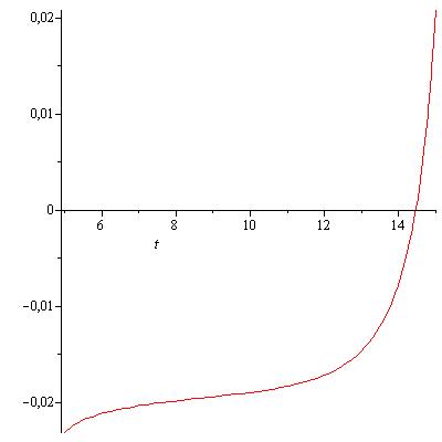
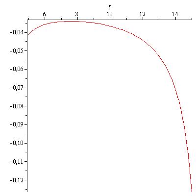
Figure 2: The density from (122) for ($\gamma=9$,$\alpha=2$) and ($\gamma=9$,$\alpha=4$), respectively. It is visible that for $\alpha=2$ the correction measure created by a perturbation is positive at the right of its support and negative at the left. For $\alpha=4$, the outlier is created, thus the correction measure is negative inside the support of its continuous part.

Example 7

In this example we will address the perturbation of the model of uniformly random domino tilings of the Aztec diamond. Let us introduce very briefly the required notions. We refer to [BK] for a detailed description of the construction below.

A signature $\lambda$ with non-negative entries can be also thought of as a Young diagram and vice versa. Two Young diagrams $\lambda,\mu$ interlace (notation $\mu\prec\lambda$) if $\lambda_{1}\geq\mu_{1}\geq\lambda_{2}\geq\mu_{2}\geq\lambda_{3}\geq\dots$ holds. Two Young diagrams interlace vertically (notation $\mu\prec_{v}\lambda$) if the conjugations of $\lambda$ and $\mu$ interlace in the sense defined above. By $|\lambda|$ one denotes the sum $\lambda_{1}+\lambda_{2}+\dots$, which is the total number of boxes in the Young diagram $\lambda$.

It is known that domino tilings of the Aztec diamond of size $M$ are in a natural bijection with the collection of Young diagrams $(\lambda^{1},\mu^{1},\dots,\lambda^{M})$ satisfying

$$\varnothing\prec\lambda^{1}\succ_{v}\mu^{1}\prec\lambda^{2}\succ_{v}\mu^{2}\prec\dots\prec\lambda^{M}\succ_{v}\varnothing.$$

Each signature $\lambda^{r}$ describes the positions of domino tilings along a one-dimensional slice of the Aztec diamond.

One can introduce a probability measure on domino tilings of the Aztec diamond in various ways. The first one is to consider the uniform measure on all tilings. Uniformly random domino tilings were extensively studied in the last thirty years, in particular, in pioneering works [JPS], [J].

We will consider a perturbation of the uniform measure. Let us view the Aztec diamond as a square, and attach to horizontal dominoes along the first (top) up-right row (if the Aztec diamond is depicted as in Figure 1) the weight $A>1$, while all the other dominoes have weight 1. Now, consider a measure on the space of domino tilings with the probability of a tiling being proportional to

$$A^{\text{number of horizontal dominoes in the first up-right row}}.$$

In terms of interlacing Young diagrams above, the probability $ZA^{|\lambda^{M}|}$ is attached to a sequence $(\lambda^{1},\mu^{1},\dots,\lambda^{M})$, where $Z$ is a normaizing constant.

For $1\leq N\leq M$, it follows from [BK, Sections 2 and 8] that the Schur generating function of the (marginal) distribution of the signature $\lambda^{N}$ under such a measure is given by

$$\prod_{i=1}^{N}\left(\frac{1+x_{i}}{2}\right)^{M-N-1}\frac{1+Ax_{i}}{1+A}.$$

To make formulas below more readable, we assume that $N=\alpha M$ exactly (without rounding up or down), where $0<\alpha<1$ is fixed. Then, as $N\to\infty$, we can apply Theorem 14 in order to study the asymptotic behavior of the signature $\lambda^{N}$: we see that the assumptions of the theorem hold with

$$\Psi(x)=\left(\frac{1}{\alpha}-1\right)\log\left(\frac{1+x}{2}\right),\qquad\Phi(x)=\log\left(\frac{1+Ax}{1+x}\right).$$

Let us assume additionally that $\alpha>\frac{1}{2}$. Performing very similar to the previous example and somewhat lengthy computations (we omit them for brevity), one arrives to the following formula for the correction measure:

$$-\mathbf{1}_{\alpha>\frac{(A+1)^{2}}{2(A^{2}+1)}}\delta\left(\frac{-1+2\alpha A-A}{\alpha(A^{2}-1)}\right)-\frac{1}{2}\mathbf{1}_{\alpha=\frac{(A+1)^{2}}{2(A^{2}+1)}}\delta\left(\frac{-1+2\alpha A-A}{\alpha(A^{2}-1)}\right)\\ +\left(\alpha+\frac{-2\alpha+1}{4y}-\frac{\alpha(2\alpha-1)}{4(\alpha y-1)}+\frac{\alpha(2A^{2}\alpha-A^{2}-2A+2\alpha-1)}{2(-\alpha y+A^{2}\alpha y-2\alpha A+1+A)}\right)\frac{\mathbf{1}_{1-(2\alpha-1)^{2}-(2\alpha y-1)^{2}>0}}{\pi\sqrt{1-(2\alpha-1)^{2}-(2\alpha y-1)^{2}}}dy.$$ (123)

As discussed in Section 1, the result explains geometric properties of a random tiling visible on Figure 1, and also it is related to another setup known as the Tangent Method for models of statistical mechanics. Formula (18) can be obtained from the formula for moments in a standard way. Note that in our assumptions (in particular, $\alpha>1/2$) outside of the arctic curve we have (the maximal possible) density 1 of particles encoded by a signature; therefore, the outlier is parameterized by a delta measure with a negative sign.

Remark 5

All general theorems in the current paper provide formulas for moments of limiting (correction) measures. In order to find their density, in all examples we perform direct calculations for finding the integral representation for moments. In this remark we outline an another approach – via Stieltjes transforms – which is comparable in complexity and can be more convenient in some other setups. We will focus on the statement of Theorem 14, a similar computation can be performed for other theorems from this paper as well.

In notations of Theorem 14, using the binomial theorem, one gets

$$\mathbf{m}^{\prime}_{k}=\frac{1}{2\pi\mathbf{i}}\oint\left(\Phi^{\prime}(x)-\frac{1}{2x}\right)\mathcal{F}(x)^{k}dx,$$

where $\mathcal{F}(x):=x\Psi^{\prime}(x)+\frac{x}{x-1}$, and the contour of integration encircles $x=1$ and no other poles of the integrand. Therefore, we have

$$-\sum_{i=0}^{\infty}\mathbf{m}^{\prime}_{k}y^{k+1}=-\frac{1}{2\pi\mathbf{i}}\oint\frac{\Phi^{\prime}(x)-\frac{1}{2x}}{y}\frac{1}{1-\frac{\mathcal{F}(x)}{y}}dx.$$ (124)

The equation $\mathcal{F}(x)=y$ has a unique solution $x_{+}(y)$ for large $|y|$ (this follows from the formal power series technique). The solution can be analytically continued to the upper half-plane. In examples, this continuation often can be given explicitly, and it is also continuous on a real line (though we do not know how to justify these steps in full generality). In such a case, the contour integral in (124) can be calculated via computing the residue at the single pole inside the contour of integration for large $|y|$, and then analytically continued. One obtains the following formula for the Stieltjes transform of the correction measure:

$$St_{\mu}(y)=\frac{\Phi^{\prime}(x_{+}(y))-\frac{1}{2x_{+}(y)}}{\mathcal{F}^{\prime}(x_{+}(y))},\qquad\Im(y)>0.$$

Thus, the formula for the density of the correction measure is given by

$$d(y)=\frac{1}{\pi}\Im\left(\frac{\Phi^{\prime}(x_{+}(y))-\frac{1}{2x_{+}(y)}}{\mathcal{F}^{\prime}(x_{+}(y))}\right),\qquad y\in\mathbb{R},$$

while outliers can be found from the condition $\Phi^{\prime}(x_{+}(y))=\infty$.

7 Second order infinitesimal free probability

In this section we analyze the third leading term in the expectation of the empirical measure of random matrices via its Harish-Chandra transform. We also connect it with notions coming from second order infinitesimal free probability.

The main result of the section is the following theorem.

Theorem 16

Let $A$ be a random Hermitian matrix of size $N$ and assume that for every finite $r$ one has

$$\lim_{N\rightarrow\infty}N^{2}\left(\frac{1}{N}\log\mathbb{E}[H\text{}C(x_{1},\ldots,x_{r},0^{N-r};\lambda_{1}(A),\ldots,\lambda_{N}(A))]-\sum_{i=1}^{r}\Psi(x_{i})-\frac{1}{N}\sum_{i=1}^{r}\Phi(x_{i})\right)=\sum_{i=1}^{r}\mathrm{T}(x_{i}),$$ (125)

where $\Psi,\Phi,\mathrm{T}$ are smooth functions in a complex neighborhood of $0$ and the above convergence is uniform in a complex neighborhood of $0^{r}$. Then the $1/N^{2}$ correction of the average empirical distribution of $N^{-1}\cdot A$ is given by

$$\lim_{N\rightarrow\infty}N^{2}\left(\frac{1}{N^{k+1}}\mathbb{E}[\operatorname{Tr}(A^{k})]-\boldsymbol{\mu}_{k}-\frac{1}{N}\boldsymbol{\mu}^{\prime}_{k}\right)=\boldsymbol{\mu}^{\prime\prime}_{k}+\boldsymbol{\nu}^{\prime\prime}_{k},$$

where $(\boldsymbol{\mu}_{k})_{k\in\mathbb{N}},(\boldsymbol{\mu}^{\prime}_{k})_{k\in\mathbb{N}}$ are given by (54),(81) respectively. The sequences $(\boldsymbol{\mu}^{\prime\prime}_{k})_{k\in\mathbb{N}},(\boldsymbol{\nu}^{\prime\prime}_{k})_{k\in\mathbb{N}}$ are given by

$$\boldsymbol{\mu}^{\prime\prime}_{k}=\sum_{m=0}^{k-1}\frac{k!}{m!(m+1)!(k-m-1)!}\left.\frac{\mathrm{d}^{m}}{\mathrm{d}x^{m}}((\Psi^{\prime}(x))^{k-m-1}\mathrm{T}^{\prime}(x))\right|_{x=0}$$

$$\text{{\hskip 100.00015pt}}+\frac{1}{2}\sum_{m=0}^{k-2}\frac{k!}{m!(m+1)!(k-m-2)!}\left.\frac{\mathrm{d}^{m}}{\mathrm{d}x^{m}}((\Psi^{\prime}(x))^{k-m-2}(\Phi^{\prime}(x))^{2})\right|_{x=0}$$ (126)

and

$$\boldsymbol{\nu}^{\prime\prime}_{k}=\frac{1}{24}\sum_{m=0}^{k-3}\frac{k!}{m!(m+1)!(k-m-3)!}\left.\frac{\mathrm{d}^{m}}{\mathrm{d}x^{m}}((\Psi^{\prime}(x))^{k-m-3}\Psi^{\prime\prime\prime}(x))\right|_{x=0}$$

$$\text{{\hskip 40.00006pt}}+\frac{1}{12}\sum_{m=0}^{k-3}\frac{k!}{m!(m+2)!(k-m-3)!}\left.\frac{\mathrm{d}^{m}}{\mathrm{d}x^{m}}((\Psi^{\prime}(x))^{k-m-3}\Psi^{\prime\prime\prime}(x))\right|_{x=0}$$

$$\text{{\hskip 100.00015pt}}+\frac{1}{12}\sum_{m=0}^{k-4}\frac{k!}{m!(m+2)!(k-m-4)!}\left.\frac{\mathrm{d}^{m}}{\mathrm{d}x^{m}}((\Psi^{\prime}(x))^{k-m-4}(\Psi^{\prime\prime}(x))^{2})\right|_{x=0}.$$ (127)

Proof.

For notation simplicity we write $f(x_{1},\ldots,x_{N})=\mathbb{E}[H\text{}C(x_{1},\ldots,x_{N};\lambda_{1}(A),\ldots,\lambda_{N}(A))]$. Note that (125) implies that the relations (40),(79) are satisfied. Thus, the empirical distribution of $N^{-1}\cdot A$ converges to a probability measure with moments $(\boldsymbol{\mu}_{k})_{k\in\mathbb{N}}$ and its $1/N$ correction is given by $(\boldsymbol{\mu}^{\prime}_{k})_{k\in\mathbb{N}}$. We have also shown an expansion

$$\frac{1}{N^{k+1}}\mathbb{E}[\operatorname{Tr}(A^{k})]=\sum_{i=0}^{k}\frac{1}{N^{i}}M_{i,N}(\Psi),$$ (128)

where $N^{2}M_{0,N}(\Psi)$ is a linear combination of terms of the form

$$N^{2}\partial_{i_{m}}\ldots\partial_{i_{1}}\left(\partial_{i_{0}}\left(\frac{1}{N}\log\text{}f\right)\right)^{k-m}(0^{N}).$$ (129)

Due to (125), for $|\{i_{0},\ldots,i_{m}\}|>1$, (129) converges to $0$ as $N\rightarrow\infty$, which implies that

$$N^{2}\left(M_{0,N}(\Psi)-\boldsymbol{\mu}_{k}-\frac{1}{N}\boldsymbol{\mu}^{\prime}_{k}\right)=\omicron(1)+N^{2}\sum_{m=0}^{k-1}\frac{k!}{m!(m+1)!(k-m)!}\times$$

$$\left(\left.\partial_{1}^{m}\left(\partial_{1}\left(\frac{1}{N}\log\text{}f\right)\right)^{k-m}(0^{N})-\frac{\mathrm{d}^{m}}{\mathrm{d}x^{m}}((\Psi^{\prime}(x))^{k-m})\right|_{x=0}-\frac{k-m}{N}\left.\frac{\mathrm{d}^{m}}{\mathrm{d}x^{m}}((\Psi^{\prime}(x))^{k-m-1}\Phi^{\prime}(x))\right|_{x=0}\right).$$

For fixed $m\in\{0,\ldots,k-1\}$, by Leibniz rule, we get

$$N^{2}\left(\partial_{1}^{m}\left(\partial_{1}\left(\frac{1}{N}\log\text{}f\right)\right)^{k-m}(0^{N})-\left.\frac{\mathrm{d}^{m}}{\mathrm{d}x^{m}}((\Psi^{\prime}(x))^{k-m})\right|_{x=0}-\frac{k-m}{N}\left.\frac{\mathrm{d}^{m}}{\mathrm{d}x^{m}}((\Psi^{\prime}(x))^{k-m-1}\Phi^{\prime}(x))\right|_{x=0}\right)$$

$$=\sum_{l_{1}+\cdots+l_{k-m}=m}\frac{m!}{l_{1}!\ldots l_{k-m}!}$$

$$\times\left(N^{2}\prod_{i=1}^{k-m}\partial_{1}^{l_{i}+1}\left(\frac{1}{N}\log\text{}f\right)(0^{N})-N^{2}\prod_{i=1}^{k-m}\Psi^{(l_{i}+1)}(0)-N\sum_{i=1}^{k-m}\Phi^{(l_{i}+1)}(0)\prod_{\underset{j\neq i}{j=1}}^{k-m}\Psi^{(l_{j}+1)}(0)\right)$$ (130)

For fixed indices $l_{1},\ldots,l_{k-m}$, due to (125), for every $i\in\{1,\ldots,k-m\}$, we have

$$\lim_{N\rightarrow\infty}N^{2}\left.\partial_{1}^{l_{i}+1}\left(\frac{1}{N}\log\text{}f\right)(0^{N})-N^{2}\Psi^{(l_{i}+1)}(0)-N\Phi^{(l_{i}+1)}(0)\right)=\mathrm{T}^{(l_{i}+1)}(0),$$

and by induction on $k-m$ we obtain

$$\lim_{N\rightarrow\infty}\left(N^{2}\prod_{i=1}^{k-m}\partial_{1}^{l_{i}+1}\left(\frac{1}{N}\log\text{}f\right)(0^{N})-N^{2}\prod_{i=1}^{k-m}\Psi^{(l_{i}+1)}(0)-N\sum_{i=1}^{k-m}\Phi^{(l_{i}+1)}(0)\prod_{\underset{j\neq i}{j=1}}^{k-m}\Psi^{(l_{j}+1)}(0)\right)$$

$$=\sum_{i=1}^{k-m}\mathrm{T}^{(l_{i}+1)}(0)\prod_{\underset{j\neq i}{j=1}}^{k-m}\Psi^{(l_{j}+1)}(0)+\frac{1}{2}\sum_{\underset{i\neq j}{i,j=1}}^{k-m}\Phi^{(l_{i}+1)}(0)\Phi^{(l_{j}+1)}(0)\prod_{\underset{r\neq i,j}{r=1}}^{k-m}\Psi^{(l_{r}+1)}(0).$$

Therefore, as $N\rightarrow\infty$, (130) converges to

$$(k-m)\left.\frac{\mathrm{d}^{m}}{\mathrm{d}x^{m}}((\Psi^{\prime}(x))^{k-m-1}\mathrm{T}^{\prime}(x))\right|_{x=0}+\frac{(k-m)\text{}(k-m-1)}{2}\left.\frac{\mathrm{d}^{m}}{\mathrm{d}x^{m}}((\Psi^{\prime}(x))^{k-m-2}(\Phi^{\prime}(x))^{2})\right|_{x=0},$$

which implies that

$$\lim_{N\rightarrow\infty}N^{2}\left(M_{0,N}(\Psi)-\boldsymbol{\mu}_{k}-\frac{1}{N}\boldsymbol{\mu}^{\prime}_{k}\right)=\boldsymbol{\mu}^{\prime\prime}_{k}.$$

Thus, the claim holds if $\lim_{N\rightarrow\infty}(N\text{}\cdot M_{1,N}(\Psi)+M_{2,N}(\Psi))=\boldsymbol{\nu}^{\prime\prime}_{k}$. The computation of $M_{1,N}(\Psi)$ was presented in the proof of Theorem 12. Taking also into account the assumption (125), we have

$$N\cdot M_{1,N}(\Psi)=\omicron(1)+\frac{N}{2}\sum_{m=0}^{k-2}\frac{k!}{m!(m+1)!(k-m-2)!}\partial_{1}^{m}\left(\left(\partial_{1}\left(\frac{1}{N}\log\text{}f\right)\right)^{k-m-2}\partial_{1}^{2}\left(\frac{1}{N}\log\text{}f\right)\right)(0^{N})$$

$$-\frac{N}{2}\sum_{m=1}^{k-1}\frac{k!}{(m-1)!m!(k-m)!}\partial_{1}^{m}\left(\partial_{1}\left(\frac{1}{N}\log\text{}f\right)\right)^{k-m}(0^{N})=\omicron(1).$$

Therefore, $\lim_{N\rightarrow\infty}N\cdot M_{1,N}(\Psi)=0$. In order to determine $M_{2,N}(\Psi)$, note that relation (40) implies that for every $k\in\mathbb{N}$, $\mathbb{E}[\operatorname{Tr}(A^{k})]$ can be written as a linear combination of terms

$$N^{l_{1}+\cdots+l_{k-m}}\binom{N}{m+1}c_{N}(m),$$ (131)

where $m\in\{0,\ldots,k-1\}$, $l_{1}+2l_{2}+\cdots+(k-m)l_{k-m}=k-m$, and $c_{N}(m)$’s are linear combinations of derivatives of the form (49). Then, $M_{2,N}(\Psi)$ is given by the sum of the summands of terms (131) with factor $N^{k-1}$. There are three cases that we have to consider regarding $l_{1},\ldots,l_{k-m}$ in order to compute these summands, since a term

$$N^{l_{1}+\cdots+l_{k-m}}\binom{N}{m+1}$$

should be a polynomial in $N$ of degree at least $k-1$. Thus, we must have $l_{1}+\cdots+l_{k-m}\in\{k-m,k-m-1,k-m-2\}$, since a binomial coefficient is a polynomial in $N$ of degree $m+1$. For each case, we are interested in the coefficient of $N^{k-1}$. For $l_{1}+\cdots+l_{k-m}=k-m-1$, i.e. $l_{1}=k-m-2$, $l_{2}=1$ and $l_{3}=\cdots=l_{k-m}=0$ the summands of the terms (131) with factor $N^{k-1}$ are

$$-N^{k-1}\left(\sum_{i=1}^{m}i\right)\left(\frac{k!}{2m!(m+1)!(k-m-2)!}\partial_{1}^{m}\left(\left(\partial_{1}\left(\frac{1}{N}\log\text{}f\right)\right)^{k-m-2}\partial_{1}^{2}\left(\frac{1}{N}\log\text{}f\right)\right)(0^{N})+\omicron(1)\right)$$

$$=-N^{k-1}\left(\frac{k!}{4(m-1)!m!(k-m-2)!}\partial_{1}^{m}\left(\left(\partial_{1}\left(\frac{1}{N}\log\text{}f\right)\right)^{k-m-2}\partial_{1}^{2}\left(\frac{1}{N}\log\text{}f\right)\right)(0^{N})+\omicron(1)\right),$$

where $m\in\{1,\ldots,k-2\}$. Thus, the contribution of these summands to $\lim_{N\rightarrow\infty}M_{2,N}(\Psi)$ will be

$$-\sum_{m=0}^{k-3}\frac{k!}{4m!(m+1)!(k-m-3)!}\left.\frac{\mathrm{d}^{m+1}}{\mathrm{d}x^{m+1}}((\Psi^{\prime}(x))^{k-m-3}\Psi^{\prime\prime}(x))\right|_{x=0}.$$ (132)

For the case $l_{1}+\cdots+l_{k-m}=k-m-2$ we have that $l_{1}=k-m-4$, $l_{2}=2$, $l_{3}=\cdots=l_{k-m}=0$ or $l_{1}=k-m-3$, $l_{3}=1$ and $l_{2}=l_{4}=\cdots=l_{k-m}=0$. For $l_{1}=k-m-4$, $l_{2}=2$ and $l_{3}=\cdots=l_{k-m}=0$, the summands of the terms (131) with factor $N^{k-1}$ are

$$N^{k-1}\left(\frac{k!}{8m!(m+1)!(k-m-4)!}\partial_{1}^{m}\left(\left(\partial_{1}\left(\frac{1}{N}\log\text{}f\right)\right)^{k-m-4}\left(\partial_{1}^{2}\left(\frac{1}{N}\log\text{}f\right)\right)^{2}\right)(0^{N})+\omicron(1)\right),$$

where $m\in\{0,\ldots,k-4\}$. On the other hand, for $l_{1}=k-m-3$, $l_{3}=1$ and $l_{2}=l_{4}=\cdots=l_{k-m}=0$, the summands of the terms (131) with factor $N^{k-1}$ are

$$N^{k-1}\left(\frac{k!}{6m!(m+1)!(k-m-3)!}\partial_{1}^{m}\left(\left(\partial_{1}\left(\frac{1}{N}\log\text{}f\right)\right)^{k-m-3}\partial_{1}^{3}\left(\frac{1}{N}\log\text{}f\right)\right)(0^{N})+\omicron(1)\right),$$

where $m\in\{0,\ldots,k-3\}$. Hence, the case $l_{1}+\cdots+l_{k-m}=k-m-2$ contributes to $\lim_{N\rightarrow\infty}M_{2,N}(\Psi)$ the expression

$$\sum_{m=0}^{k-4}\frac{k!}{8m!(m+1)!(k-m-4)!}\left.\frac{\mathrm{d}^{m}}{\mathrm{d}x^{m}}((\Psi^{\prime}(x))^{k-m-4}(\Psi^{\prime\prime}(x))^{2})\right|_{x=0}$$

$$\text{{\hskip 100.00015pt}}+\sum_{m=0}^{k-3}\frac{k!}{6m!(m+1)!(k-m-3)!}\left.\frac{\mathrm{d}^{m}}{\mathrm{d}x^{m}}((\Psi^{\prime}(x))^{k-m-3}\Psi^{\prime\prime\prime}(x))\right|_{x=0}.$$ (133)

For the last case $l_{1}+\cdots+l_{k-m}=k-m$, we have $l_{1}=k-m$ and $l_{2}=\cdots=l_{k-m}=0$. Then, the desired summands will be

$$N^{k-1}\left(\frac{1}{2}\sum_{\underset{i\neq j}{i,j=0}}^{m}i\text{}j\right)\left(\frac{k!}{m!(m+1)!(k-m)!}\partial_{1}^{m}\left(\partial_{1}\left(\frac{1}{N}\log\text{}f\right)\right)^{k-m}(0^{N})+\omicron(1)\right)$$

$$\text{{\hskip 40.00006pt}}=N^{k-1}\frac{k!}{8(m-2)!(m-1)!(k-m)!}\partial_{1}^{m}\left(\partial_{1}\left(\frac{1}{N}\log\text{}f\right)\right)^{k-m}(0^{N})$$

$$\text{{\hskip 80.00012pt}}+N^{k-1}\frac{k!}{12(m-2)!m!(k-m)!}\partial_{1}^{m}\left(\partial_{1}\left(\frac{1}{N}\log\text{}f\right)\right)^{k-m}(0^{N})+N^{k-1}\omicron(1),$$

where $m\in\{2,\ldots,k-1\}$. Thus, the contribution of these summands to $\lim_{N\rightarrow\infty}M_{2,N}(\Psi)$ will be equal to

$$\sum_{m=0}^{k-3}\left(\frac{k!}{8m!(m+1)!(k-m-2)!}+\frac{k!}{12m!(m+2)!(k-m-2)!}\right)\left.\frac{\mathrm{d}^{m+2}}{\mathrm{d}x^{m+2}}((\Psi^{\prime}(x))^{k-m-2})\right|_{x=0}.$$ (134)

Since $\lim_{N\rightarrow\infty}M_{2,N}(\Psi)$ is equal to the sum of (132),(133) and (134), a straightforward computation shows that the limit is equal to $\boldsymbol{\nu}^{\prime\prime}_{k}$. This proves the claim. ∎

We would like to better understand the terms $\boldsymbol{\mu}^{\prime\prime}_{k},\boldsymbol{\nu}^{\prime\prime}_{k}$ from Theorem 16. In the proof of Theorem 16 we showed that $\boldsymbol{\nu}^{\prime\prime}_{k}=\lim_{N\rightarrow\infty}M_{2,N}(\Psi)$, and that $\boldsymbol{\mu}^{\prime\prime}_{k}$ contributes to the $1/N^{2}$ correction of $A/N$ due to the relation

$$\boldsymbol{\mu}^{\prime\prime}_{k}=\lim_{N\rightarrow\infty}N^{2}\left(M_{0,N}(\Psi)-\boldsymbol{\mu}_{k}-\frac{1}{N}\boldsymbol{\mu}^{\prime}_{k}\right).$$

However, we would like to provide also a different explanation of the term $\boldsymbol{\mu}^{\prime\prime}_{k}$, which makes the connection with second order infinitesimal free probability. This connection is a generalization of the fact that the formula (81) for the $1/N$ correction of $A/N$ gives an explicit description for the infinitesimal free cumulants of the infinitesimal non-commutative probability space $(\mathbb{C}\langle\mathbf{x}\rangle,\varphi,\varphi^{\prime})$, where for every $P\in\mathbb{C}\langle\mathbf{x}\rangle$

$$\varphi(P)=\lim_{N\rightarrow\infty}\frac{1}{N}\mathbb{E}[\operatorname{Tr}\text{}P(N^{-1}\cdot A)]\text{\quad and\quad}\varphi^{\prime}(P)=\lim_{N\rightarrow\infty}N\left(\frac{1}{N}\mathbb{E}[\operatorname{Tr}\text{}P(N^{-1}\cdot A)]-\varphi(P)\right).$$

By the above equalities, $\mu_{k}=\varphi(\mathbf{x}^{k})$ and $\boldsymbol{\mu}^{\prime}_{k}=\varphi^{\prime}(\mathbf{x}^{k})$, for every $k\in\mathbb{N}$. The role of functions $\Psi,\Phi$ in the computation of infinitesimal free cumulants can be seen from (90) and (91). Thus, thinking of $\boldsymbol{\mu}_{k},\boldsymbol{\mu}^{\prime}_{k}$ as moments, we have that the relations (54),(81) describe moment-cumulant relations for an infinitesimal non-commutative probability space of order 1. The fact that $\boldsymbol{\mu}^{\prime\prime}_{k}$ is determined by (126) allows us to go a step further and see the relations (54),(81),(126) as moment-cumulant relations, in the sense of Definition 4, for an infinitesimal non-commutative probability space of order 2. This is shown by the next lemma.

Lemma 7

Let $\Psi,\Phi,\mathrm{T}$ be infinitely differentiable functions at $0$ and consider the sequences $(c_{n})_{n\in\mathbb{N}},(c^{\prime}_{n})_{n\in\mathbb{N}},(c^{\prime\prime}_{n})_{n\in\mathbb{N}}$, where for every $n\in\mathbb{N}$

$$c_{n}:=\frac{\Psi^{(n)}(0)}{(n-1)!},\text{\quad}c^{\prime}_{n}:=\frac{\Phi^{(n)}(0)}{(n-1)!}\text{\quad and\quad}c^{\prime\prime}_{n}:=2\frac{\mathrm{T}^{(n)}(0)}{(n-1)!}.$$

Then for the sequence $(\boldsymbol{\mu}^{\prime\prime}_{k})_{k\in\mathbb{N}}$ defined by (126), for every $k\in\mathbb{N}$, we have

$$\boldsymbol{\mu}^{\prime\prime}_{k}=\frac{1}{2}\left(\sum_{\pi\in\operatorname{NC}(k)}\sum_{V\in\pi}c^{\prime\prime}_{|V|}\prod_{\underset{W\neq V}{W\in\pi}}c_{|W|}+\sum_{\pi\in\operatorname{NC}(k)}\sum_{\underset{W\neq V}{V,W\in\pi}}c^{\prime}_{|V|}c^{\prime}_{|W|}\prod_{\underset{U\neq V,W}{U\in\pi}}c_{|U|}\right).$$

Proof.

In Lemma 5 we proved, for every $k\in\mathbb{N}$, that

$$\sum_{m=0}^{k-1}\frac{k!}{m!(m+1)!(k-m-1)!}\left.\frac{\mathrm{d}^{m}}{\mathrm{d}x^{m}}((\Psi^{\prime}(x))^{k-m-1}\mathrm{T}^{\prime}(x))\right|_{x=0}=\frac{1}{2}\sum_{\pi\in\operatorname{NC}(k)}\sum_{V\in\pi}c^{\prime\prime}_{|V|}\prod_{\underset{W\neq V}{W\in\pi}}c_{|W|}.$$

Thus, it suffices to show that

$$\sum_{m=0}^{k-2}\frac{k!}{m!(m+1)!(k-m-2)!}\left.\frac{\mathrm{d}^{m}}{\mathrm{d}x^{m}}((\Psi^{\prime}(x))^{k-m-2}(\Phi^{\prime}(x))^{2})\right|_{x=0}=\sum_{\pi\in\operatorname{NC}(k)}\sum_{\underset{W\neq V}{V,W\in\pi}}c^{\prime}_{|V|}c^{\prime}_{|W|}\prod_{\underset{U\neq V,W}{U\in\pi}}c_{|U|}.$$ (135)

By Leibniz rule, the left hand side of (135) is equal to

$$\sum_{m=0}^{k-2}\sum_{l_{1+\cdots+l_{k-m}=m}}\frac{k!}{(m+1)!(k-m-2)!\prod_{i=1}^{k-m}l_{i}!}\Phi^{(l_{k-m}+1)}(0)\Phi^{(l_{k-m-1}+1)}(0)\prod_{i=1}^{k-m-2}\Psi^{(l_{i}+1)}(0).$$ (136)

The way that we related $(k-m)$-tuples $(l_{1},\ldots,l_{k-m})$ such that $l_{1}+\cdots+l_{k-m}=m$ with non-crossing partitions $\pi=\{V_{1},\ldots,V_{k-m}\}\in\operatorname{NC}(k)$ in Lemma 5 will lead to the equality (135). In more detail, for $m\in\{0,\ldots,k-2\}$, consider non-negative integers $\lambda_{1},\ldots,\lambda_{k-m}$ such that $\lambda_{1}+\cdots+\lambda_{k-m}=m$. We also assume that $\{\lambda_{1},\ldots,\lambda_{k-m}\}=\{\nu_{1},\ldots,\nu_{a}\}$, where $\nu_{i}\neq\nu_{j}$, for every $i\neq j$, and we define for every $i\in\{1,\ldots,a\}$

$$r_{i}:=|\{j=1,\ldots,k-m:\lambda_{j}=\nu_{i}\}|.$$

We would like to calculate the contribution of $(\lambda_{1},\ldots,\lambda_{k-m})$ to the latter sum of (136). In order to do so, we consider two cases. If we assume $l_{k-m}\neq l_{k-m-1}$, the $(k-m)$-tuple $(\lambda_{1},\ldots,\lambda_{k-m})$ contributes terms of the form

$$\frac{k!}{(m+1)!(k-m-2)!\prod_{t=1}^{k-m}\lambda_{t}!}\Phi^{(\nu_{i}+1)}(0)\Phi^{(\nu_{j}+1)}(0)(\Psi^{(\nu_{i}+1)}(0))^{r_{i}-1}(\Psi^{(\nu_{j}+1)}(0))^{r_{j}-1}\prod_{\underset{t\neq i,j}{t=1}}^{a}(\Psi^{(\nu_{t}+1)}(0))^{r_{t}},$$

where $i,j\in\{1,\ldots,a\}$, with $i<j$. The number of times that such a term will appear in the latter sum of (136) is equal to the number of different ways that we can cover $k-m-2$ points on a line segment with $r_{t}$ number of elements $\nu_{t}$ ($t\in\{1,\ldots,a\}\backslash\{i,j\}$), $r_{i}-1$ number of elements $\nu_{i}$ and $r_{j}-1$ number of elements $\nu_{j}$. This is equal to

$$C_{i,j}:=\frac{(k-m-2)!}{r_{1}!\ldots r_{i-1}!(r_{i}-1)!r_{i+1}!\ldots r_{j-1}!(r_{j}-1)!r_{j+1}!\ldots r_{a}!}.$$

Thus, we see that the $(k-m)$-tuple $(\lambda_{1},\ldots,\lambda_{k-m})$ contributes to the latter sum of (136) the expression

$$2\frac{k!}{(m+1)!(k-m-2)!\prod_{t=1}^{a}(\nu_{t}!)^{r_{t}}}\sum_{\underset{i<j}{i,j=1}}^{a}C_{i,j}\Phi^{(\nu_{i}+1)}(0)\Phi^{(\nu_{j}+1)}(0)(\Psi^{(\nu_{i}+1)}(0))^{r_{i}-1}(\Psi^{(\nu_{j}+1)}(0))^{r_{j}-1}\prod_{\underset{t\neq i,j}{t=1}}^{a}(\Psi^{(\nu_{t}+1)}(0))^{r_{t}}.$$

By the definition of $(c_{n})_{n\in\mathbb{N}},(c^{\prime}_{n})_{n\in\mathbb{N}}$ this is equal to

$$\frac{k!}{(m+1)!\prod_{i=1}^{a}r_{i}!}\sum_{\underset{i\neq j}{i,j=1}}^{a}r_{i}r_{j}c^{\prime}_{\nu_{i}+1}c^{\prime}_{\nu_{j}+1}(c_{\nu_{i}+1})^{r_{i}-1}(c_{\nu_{j}+1})^{r_{j}-1}\prod_{\underset{t\neq i,j}{t=1}}^{a}(c_{\nu_{t}+1})^{r_{t}}.$$ (137)

In the second case, for $l_{k-m}=l_{k-m-1}$, the contributions of $(\lambda_{1},\ldots,\lambda_{k-m})$ to the latter sum of (136) will be of the form

$$\frac{k!}{(m+1)!(k-m-2)!\prod_{i=1}^{k-m}\lambda_{i}!}(\Phi^{(\nu_{j}+1)}(0))^{2}(\Psi^{(\nu_{j}+1)}(0))^{r_{j}-2}\prod_{\underset{i\neq j}{i=1}}^{a}(\Psi^{(\nu_{i}+1)}(0))^{r_{i}},$$

for some $j\in\{1,\ldots,a\}$. The number of times that this term will appear in the latter sum of (136) is equal to the number of different ways that we can cover $k-m-2$ points on a line segment with $r_{i}$ number of elements $\nu_{i}$ ($i\in\{1,\ldots,a\}\backslash\{j\}$) and $r_{j}-2$ number of elements $\nu_{j}$, i.e.

$$\frac{(k-m-2)!}{r_{1}!\ldots r_{j-1}!(r_{j}-2)!r_{j+1}!\ldots r_{a}!}.$$

Thus, $(\lambda_{1},\ldots,\lambda_{k-m})$ will further contribute to the latter sum of (136) the expression

$$\frac{k!}{(m+1)!\prod_{i=1}^{a}(\nu_{i}!)^{r_{i}}}\sum_{i=1}^{a}\frac{(\Phi^{(\nu_{i}+1)}(0))^{2}(\Psi^{(\nu_{i}+1)}(0))^{r_{i}-2}}{r_{1}!\ldots r_{i-1}!(r_{i}-2)!r_{i+1}!\ldots r_{a}!}\prod_{\underset{j\neq i}{j=1}}^{a}(\Psi^{(\nu_{j}+1)}(0))^{r_{j}}$$

$$=\frac{k!}{(m+1)!\prod_{i=1}^{a}r_{i}!}\sum_{i=1}^{a}r_{i}(r_{i}-1)(c^{\prime}_{\nu_{i}+1})^{2}(c_{\nu_{i}+1})^{r_{i}-2}\prod_{\underset{j\neq i}{j=1}}^{a}(c_{\nu_{j}+1})^{r_{j}}.$$ (138)

The total contribution of $(\lambda_{1},\ldots,\lambda_{k-m})$ is given by the sum of (137) and (138).

Regarding the right hand side of (135), a partition $\pi=\{V_{1},\ldots,V_{k-m}\}\in\operatorname{NC}(k)$ which has $r_{1}$ blocks with $\nu_{1}+1$ elements,…, $r_{a}$ blocks with $\nu_{a}+1$ elements, contributes

$$\sum_{\underset{i\neq j}{i,j=1}}^{k-m}c^{\prime}_{|V_{i}|}c^{\prime}_{|V_{j}|}\prod_{\underset{t\neq i,j}{t=1}}^{k-m}c_{|V_{t}|}=\sum_{\underset{i\neq j\text{ and }|V_{i}|=|V_{j}|}{i,j=1}}^{k-m}c^{\prime}_{|V_{i}|}c^{\prime}_{|V_{j}|}\prod_{\underset{t\neq i,j}{t=1}}^{k-m}c_{|V_{t}|}+\sum_{\underset{|V_{i}|\neq|V_{j}|}{i,j=1}}^{k-m}c^{\prime}_{|V_{i}|}c^{\prime}_{|V_{j}|}\prod_{\underset{t\neq i,j}{t=1}}^{k-m}c_{|V_{t}|}$$

$$=\sum_{i=1}^{a}r_{i}(r_{i}-1)(c^{\prime}_{\nu_{i}+1})^{2}(c_{\nu_{i}+1})^{r_{i}-2}\prod_{\underset{j\neq i}{j=1}}^{a}(c_{\nu_{j}+1})^{r_{j}}+\sum_{\underset{i\neq j}{i,j=1}}^{a}r_{i}r_{j}c^{\prime}_{\nu_{i}+1}c^{\prime}_{\nu_{j}+1}(c_{\nu_{i}+1})^{r_{i}-1}(c_{\nu_{j}+1})^{r_{j}-1}\prod_{\underset{t\neq i,j}{t=1}}^{a}(c_{\nu_{t}+1})^{r_{t}}.$$

Since the number of such partitions is equal to $\left((m+1)!\prod_{i=1}^{a}r_{i}!\right)^{-1}k!$, this proves (135) and the claim holds. ∎

In the remainder of this section we make some explicit computations, which illustrate how second order fluctuations of random matrix models are described by certain signed measures on $\mathbb{R}$. Our models consist of additive perturbations of ergodic unitarily invariant matrices.

Example 8

We consider the Hermitian random matrix of size $N$, $A=N\cdot A_{1}+\sqrt{N}A_{2}+A_{3}$, where $A_{1},A_{2},A_{3}$ are independent GUE matrices. As a consequence, for every $H\in H(N)$, one has

$$\mathbb{E}[\exp(\operatorname{Tr}(H\text{}A))]=\prod_{x\in\operatorname{Spec}(H)}\exp\left(N\frac{x^{2}}{2}+\frac{x^{2}}{2}+\frac{1}{N}\frac{x^{2}}{2}\right).$$

The $1/N^{2}$ correction of the matrix $A_{1}$ is given by

$$\frac{1}{12}\sum_{m=0}^{k-4}\frac{k!}{m!(m+2)!(k-m-4)!}\left.\frac{\mathrm{d}^{m}}{\mathrm{d}x^{m}}(x^{k-m-4})\right|_{x=0}=\frac{k(k-1)}{24\pi\mathrm{i}}\sum_{m=0}^{k-4}\binom{k-2}{m+2}\oint_{|z|=1}\frac{z^{k-m-4}}{z^{m+1}}d\text{}z$$

$$=\frac{k(k-1)}{24\pi\mathrm{i}}\oint_{|z|=1}z^{k-1}\sum_{m=2}^{k-2}\binom{k-2}{m}\left(\frac{1}{z^{2}}\right)^{m}d\text{}z=\frac{k(k-1)}{24\pi\mathrm{i}}\oint_{|z|=1}z\left(z+\frac{1}{z}\right)^{k-2}d\text{}z$$

for every $k\geq 4$. Using the change of variables $u=2\cos\text{}t$ in order to compute the last contour integral, we see that the second order correction functional of $A_{1}$

$$\phi^{\prime\prime}(P):=\lim_{N\rightarrow\infty}N^{2}\left(\frac{1}{N}\mathbb{E}[\operatorname{Tr}\text{}P(A_{1})]-\frac{1}{2\pi}\int_{-2}^{2}P(t)\sqrt{4-t^{2}}d\text{}t\right)\text{, \quad}P\in\mathbb{C}\langle\mathbf{x}\rangle,$$

is equal to

$$\phi^{\prime\prime}(P)=\frac{1}{24\pi}\int_{-2}^{2}P^{\prime\prime}(t)\frac{t^{2}-2}{\sqrt{4-t^{2}}}d\text{}t,\text{\quad for every }P\in\mathbb{C}\langle\mathbf{x}\rangle.$$

A similar formula for the second order correction functional of $A_{1}+\frac{1}{\sqrt{N}}A_{2}+\frac{1}{N}A_{3}$ can be derived if we consider an integral representation for the terms that correspond to the infinitesimal non-commutative probability space of order $2$. One of this terms is

$$\frac{1}{2}\sum_{m=0}^{k-2}\frac{k!}{m!(m+1)!(k-m-2)!}\left.\frac{\mathrm{d}^{m}}{\mathrm{d}x^{m}}(x^{k-m})\right|_{x=0}=\frac{k}{4\pi\mathrm{i}}\sum_{m=0}^{k-2}\binom{k-1}{m+1}\oint_{|z|=1}\frac{z^{k-m}}{z^{m+1}}d\text{}z$$

$$=\frac{k}{4\pi\mathrm{i}}\oint_{|z|=1}z^{k+1}\sum_{m=1}^{k-1}\binom{k-1}{m}\left(\frac{1}{z^{2}}\right)^{m}d\text{}z=\frac{k}{4\pi\mathrm{i}}\oint_{|z|=1}z^{2}\left(z+\frac{1}{z}\right)^{k-1}d\text{}z,$$

for every $k\geq 2$. The remaining term is the first order correction of $A_{1}+\frac{1}{\sqrt{N}}A_{2}$ and it was studied in Example 2. Concluding, the second order correction functional $\varphi^{\prime\prime}$ of $A_{1}+\frac{1}{\sqrt{N}}A_{2}+\frac{1}{N}A_{3}$ is given by

$$\varphi^{\prime\prime}(P)=\frac{1}{2\pi}\int_{-2}^{2}\left(P^{\prime\prime}(t)\frac{t^{2}-2}{12}+P^{\prime}(t)\frac{t^{3}-3t}{2}+P(t)(t^{2}-2)\right)\frac{1}{\sqrt{4-t^{2}}}d\text{}t,\text{\quad for every }P\in\mathbb{C}\langle\mathbf{x}\rangle.$$

Example 9

We consider the random matrix

$$A=N\cdot G+\theta_{1}X\text{}X^{\ast}+\frac{\theta_{2}}{N}Y\text{}Y^{\ast},$$ (139)

where the matrices $G,X,Y$ are independent, $G$ is a GUE of size $N$ and $X,Y$ are independent $N\times 1$ vectors with standard complex Gaussian i.i.d. entries. Then, in notation of Theorem 16, we have that

$$\Psi(x)=\frac{x^{2}}{2},\text{{\hskip 30.00005pt}}\Phi(x)=\log(1-\theta_{1}x)^{-1},\text{{\hskip 30.00005pt}}\mathrm{T}(x)=\theta_{2}x.$$

Applying the theorem and performing very similar to previous examples calculations, one arrives to the following answer for the corrections. Consider the infinitesimal non-commutative probability space of order 2, $(\mathbb{C}\langle X\rangle,\varphi^{(0)},\varphi^{(1)},\varphi^{(2)})$, where $\varphi^{(0)}$ is the limit, $\varphi^{(1)}$ is the first order correction and $\varphi^{(2)}$ is the second order correction. Then we have that

$$\varphi^{(1)}(P)=\boldsymbol{1}_{|\theta_{1}|\geq 1}\cdot P(\theta_{1}+\theta_{1}^{-1})-\frac{1}{2\pi}\int_{-2}^{2}\frac{t-2\theta_{1}}{(t-\theta_{1}-\theta_{1}^{-1})\sqrt{4-t^{2}}}P(t)d\text{}t,$$

and

$$\varphi^{(2)}(P)=\frac{\theta_{2}}{2\pi}\int_{-2}^{2}\sqrt{4-t^{2}}P^{\prime}(t)d\text{}t+\frac{1}{2\pi}\int_{-2}^{2}\frac{\theta_{1}^{2}}{\sqrt{4-t^{2}}}\frac{P^{\prime}(t)-P^{\prime}(\theta_{1}+\theta^{-1}_{1})}{t-\theta_{1}-\theta_{1}^{-1}}d\text{}t$$

$$-\frac{1}{4\pi}\int_{-2}^{2}\frac{(\theta_{1}^{2}-1)(t-2\theta_{1})}{(t-\theta_{1}-\theta_{1}^{-1})\sqrt{4-t^{2}}}\left(\frac{P^{\prime}(t)-P^{\prime}(\theta_{1}+\theta_{1}^{-1})}{t-\theta_{1}-\theta_{1}^{-1}}-P^{\prime\prime}(\theta_{1}+\theta_{1}^{-1})\right)d\text{}t+\frac{1}{24\pi}\int_{-2}^{2}P^{\prime\prime}(t)\frac{t^{2}-2}{\sqrt{4-t^{2}}}d\text{}t.$$

Instead of $\frac{\theta_{2}}{N}Y\text{}Y^{\ast}$ in (139), one can consider the deterministic Hermitian matrix with one non-zero eigenvalue $\theta_{2}$. This would lead to the same result for corrections.

8 Higher order infinitesimal free probability

In this section we present our most general result, focusing on corrections of arbitrary order of certain random matrices. Our goal is to provide explicit computations that allow us to make the connection with non-crossing cumulant functionals of $k$-th order. As before, we are interested in an asymptotic expansion

$$\frac{1}{N^{k+1}}\mathbb{E}[\operatorname{Tr}(A^{k})]=\sum_{i=0}^{k}\frac{1}{N^{i}}M_{i,N}(\Psi),$$ (140)

where $(M_{i,N}(\Psi))_{N\in\mathbb{N}}$ converges for every $i$. We would like to understand under which further conditions on $A$ one can control the terms $M_{i,N}(\Psi)$, for $i\in\{0,\ldots,k\}$, as $N\rightarrow\infty$.

Theorem 17

Let $n$ be a fixed integer. Let $A$ be a random Hermitian matrix of size $N$ and assume that for every finite $r$ one has

$$\lim_{N\rightarrow\infty}N^{n\varepsilon}\left(\frac{1}{N}\log\mathbb{E}[H\text{}C(x_{1},\ldots,x_{r},0^{N-r};\lambda_{1}(A),\ldots,\lambda_{n}(A))]-\sum_{j=0}^{n-1}\sum_{i=0}^{r}\frac{1}{N^{j\varepsilon}}\Psi_{j}(x_{i})\right)=\sum_{i=1}^{r}\Psi_{n}(x_{i}),$$ (141)

where $\Psi_{0},\ldots,\Psi_{n}$ are smooth functions in a complex neighborhood of $0$, the above convergence is uniform in a complex neighborhood of $0^{r}$ and $0<\varepsilon<n^{-1}$. Then the $1/N^{n\varepsilon}$ correction of the average empirical distribution of $N^{-1}A$ is given by

$$\lim_{N\rightarrow\infty}N^{n\varepsilon}\left(\frac{1}{N^{k+1}}\mathbb{E}[\operatorname{Tr}(A^{k})]-\sum_{j=0}^{n-1}\frac{1}{N^{j\varepsilon}}\boldsymbol{\mu}^{(j)}_{k}\right)=\boldsymbol{\mu}_{k}^{(n)},$$ (142)

where for every $j\in\{0,\ldots,n\}$

$$\boldsymbol{\mu}^{(j)}_{k}:=\sum_{b_{1}+2b_{2}+\cdots+j\text{}b_{j}=j}\sum_{m=0}^{k-b_{1}-\cdots-b_{j}}\frac{k!}{m!(m+1)!(k-m-b_{1}-\cdots-b_{j})!b_{1}!\ldots b_{j}!}\text{{\hskip 80.00012pt}}$$

$$\text{{\hskip 140.00021pt}}\times\left.\frac{\mathrm{d}^{m}}{\mathrm{d}x^{m}}((\Psi^{\prime}_{0}(x))^{k-m-b_{1}-\cdots-b_{j}}(\Psi^{\prime}_{1}(x))^{b_{1}}\ldots(\Psi^{\prime}_{j}(x))^{b_{j}})\right|_{x=0}.$$ (143)

Proof.

First, we consider an easier case, in which we additionally assume that

$$N^{n\varepsilon}\left(\frac{1}{N}\log\mathbb{E}[H\text{}C(x_{1},\ldots,x_{N};\lambda_{1}(A),\ldots,\lambda_{N}(\mathrm{A}))]-\sum_{j=0}^{n-1}\sum_{i=0}^{N}\frac{1}{N^{j\varepsilon}}\Psi_{j}(x_{i})\right)=\sum_{i=1}^{N}\Psi_{n}(x_{i}),$$ (144)

for every $N\in\mathbb{N}$ and $x_{1},\ldots,x_{N}\in\mathbb{R}$. Thus, denoting the average Harish-Chandra integral of $A$ by $f_{N}$, we have that $f_{N}=f_{0}f_{1}\ldots f_{n}$, where

$$f_{j}(x_{1},\ldots,x_{N})=\exp\left(N^{1-j\varepsilon}\sum_{i=1}^{N}\Psi_{j}(x_{i})\right),$$

for $j=0,\ldots,n$. Similarly to previous theorems, we will pass from the Harish-Chandra integral of $A$ to the $k$-th moment of the average empirical distribution of $A/N$ using the differential operator $\mathcal{D}_{k}$. We have that $\mathbb{E}(\operatorname{Tr}(A^{k}))=\mathcal{D}_{k}f_{N}|_{x_{i}=0}$ and

$$\mathcal{D}_{k}f_{N}=\sum_{m=0}^{k-1}\sum_{\underset{l_{i}\neq l_{j}\text{ for }i\neq j}{l_{0},\ldots,l_{m}=1}}^{N}\sum_{b_{0}+\cdots+b_{n}=k-m}\binom{k}{m}\frac{(k-m)!}{b_{0}!\ldots b_{n}!}\frac{\partial_{l_{0}}^{b_{0}}f_{0}\partial_{l_{0}}^{b_{1}}f_{1}\ldots\partial^{b_{n}}_{l_{0}}f_{n}}{(x_{l_{0}}-x_{l_{1}})\ldots(x_{l_{0}}-x_{l_{m}})}.$$ (145)

As a consequence, $\mathcal{D}_{k}f_{N}$ is a linear combination of terms

$$\text{{\hskip 30.00005pt}}f_{N}\frac{\prod_{i=0}^{n}\prod_{j=1}^{b_{i}}(\Psi_{i}^{(j)}(x_{l_{0}}))^{\lambda_{i,j}}}{(x_{l_{0}}-x_{l_{1}})\ldots(x_{l_{0}}-x_{l_{m}})}+f_{N}\frac{\prod_{i=0}^{n}\prod_{j=1}^{b_{i}}(\Psi_{i}^{(j)}(x_{l_{1}}))^{\lambda_{i,j}}}{(x_{l_{1}}-x_{l_{0}})(x_{l_{1}}-x_{l_{2}})\ldots(x_{l_{1}}-x_{l_{m}})}+\ldots+f_{N}\frac{\prod_{i=0}^{n}\prod_{j=1}^{b_{i}}(\Psi_{i}^{(j)}(x_{l_{m}}))^{\lambda_{i,j}}}{(x_{l_{m}}-x_{l_{0}})\ldots(x_{l_{m}}-x_{l_{m-1}})},$$ (146)

where these terms have a limit for $x_{1}=\cdots=x_{N}=0$, due to Lemma 3. Note that all the coefficients in $\mathcal{D}_{k}f_{N}|_{x_{i}=0}$ will be of order $O(N^{k+1})$. In order to prove the claim, for $x_{1}=\cdots=x_{N}=0$ we have to compute the terms (146), where their coefficients are not $\omicron(N^{k+1-n\varepsilon})$. Since $0<\varepsilon<n^{-1}$ and $b_{0}+\cdots+b_{n}=k-m$, note that differentiating the functions $f_{0},\ldots,f_{n}$ in the expression

$$\binom{k}{m}\frac{(k-m)!}{b_{0}!\ldots b_{n}!}\frac{\partial_{l_{0}}^{b_{0}}f_{0}\partial_{l_{0}}^{b_{1}}f_{1}\ldots\partial_{l_{0}}^{b_{n}}f_{n}}{(x_{l_{0}}-x_{l_{1}})\ldots(x_{l_{0}}-x_{l_{m}})}$$

can be written as a sum, where only the summand

$$\frac{k!}{m!b_{0}!\ldots b_{n}!}N^{b_{0}+b_{1}(1-\varepsilon)+\cdots+b_{n}(1-n\varepsilon)}f_{N}\frac{(\Psi^{\prime}_{0}(x_{l_{0}}))^{b_{0}}\ldots(\Psi^{\prime}_{n}(x_{l_{0}}))^{b_{n}}}{(x_{l_{0}}-x_{l_{1}})\ldots(x_{l_{0}}-x_{l_{m}})}$$

may contribute to a term (146) with a coefficient that is not $\omicron(N^{k+1-n\varepsilon})$. Indeed, it follows from the equality

$$\lim_{x_{1},\ldots,x_{N}\rightarrow 0}\left(\frac{(\Psi^{\prime}_{0}(x_{l_{0}}))^{b_{0}}\ldots(\Psi^{\prime}_{n}(x_{l_{0}}))^{b_{n}}}{(x_{l_{0}}-x_{l_{1}})\ldots(x_{l_{0}}-x_{l_{m}})}+\frac{(\Psi^{\prime}_{0}(x_{l_{1}}))^{b_{0}}\ldots(\Psi^{\prime}_{n}(x_{l_{1}}))^{b_{n}}}{(x_{l_{1}}-x_{l_{0}})(x_{l_{1}}-x_{l_{2}})\ldots(x_{l_{1}}-x_{l_{m}})}+\right.\text{{\hskip 80.00012pt}}$$

$$\text{{\hskip 80.00012pt}}\left.\ldots+\frac{(\Psi^{\prime}_{0}(x_{l_{m}}))^{b_{0}}\ldots(\Psi^{\prime}_{n}(x_{l_{m}}))^{b_{n}}}{(x_{l_{m}}-x_{l_{0}})\ldots(x_{l_{m}}-x_{l_{m-1}})}\right)=\frac{1}{m!}\left.\frac{\mathrm{d}^{m}}{\mathrm{d}x^{m}}((\Psi^{\prime}_{0}(x))^{b_{0}}\ldots(\Psi^{\prime}_{n}(x))^{b_{n}})\right|_{x=0},$$

in which the right hand side does not depend on $l_{0},\ldots,l_{m}\in\{1,\ldots,N\}$. Thus, the above limit appears in the right hand side of (145) exactly $m!\binom{N}{m+1}$ times. Therefore, the summands (146) of $\mathcal{D}_{k}f_{N}|_{x_{i}=0}$ with a coefficient that it is not $\omicron(N^{k+1-n\varepsilon})$ have the form

$$\frac{k!}{m!(m+1)!b_{0}!\ldots b_{n}!}N^{k+1-b_{1}\varepsilon-\cdots-n\text{}b_{n}\varepsilon}\left.\frac{\mathrm{d}^{m}}{\mathrm{d}x^{m}}((\Psi^{\prime}_{0}(x))^{b_{0}}\ldots(\Psi^{\prime}_{n}(x))^{b_{n}})\right|_{x=0},$$ (147)

where $b_{0}=k-m-b_{1}-\cdots-b_{n}$ and $b_{1}+2b_{2}+\cdots+n\text{}b_{n}\leq n$. Thus, the summands that we are interested in have a factor $N^{k+1-j\varepsilon}$, for $j=0,\ldots,n$. Taking the sum of those of the form (147) with the same factor $N^{k+1-j\varepsilon}$ (i.e., for $b_{1}+2b_{2}+\cdots+jb_{j}=j$, $b_{j+1}=\cdots=b_{n}=0$, and $m=0,\ldots,k-b_{1}-\cdots-b_{j}$), we get that

$$\frac{1}{N^{k+1}}\mathbb{E}[\operatorname{Tr}(A^{k})]=\frac{1}{N^{k+1}}\mathcal{D}_{k}(f_{0}\ldots f_{n})|_{x_{i}=0}=\boldsymbol{\mu}_{k}^{(0)}+\frac{1}{N^{\varepsilon}}\boldsymbol{\mu}_{k}^{(1)}+\cdots+\frac{1}{N^{n\varepsilon}}\boldsymbol{\mu}_{k}^{(n)}+o(N^{-n\varepsilon}),$$ (148)

and the claim holds.

Now we deal with a more general case, in which only relation (141) is known for $A$. Again, we will use the differential operator $\mathcal{D}_{k}$ in order to pass from the Harish-Chandra integral of $A$ to the $k$-th moment of the average empirical distribution of $A/N$. Taking into account (141), it will be useful for our analysis to write the average Harish-Chandra integral as $f_{N}=F_{N}\cdot G_{N}$, where $F_{N}:=\exp(N\cdot\widetilde{F_{N}})$, where

$$\widetilde{F_{N}}(x_{1},\ldots,x_{N}):=\frac{1}{N}\log\text{}f_{N}(x_{1},\ldots,x_{N})-\sum_{j=0}^{n}\sum_{i=1}^{N}\frac{1}{N^{j\varepsilon}}\Psi_{j}(x_{i})$$

and

$$G_{N}(x_{1},\ldots,x_{N}):=\prod_{j=0}^{n}\exp\left(N^{1-j\varepsilon}\sum_{i=1}^{N}\Psi_{j}(x_{i})\right).$$

We write $G_{N}=f_{0}f_{1}\ldots f_{n}$, where $f_{j}:=\exp(N^{1-j\varepsilon}g_{j})$ and $g_{j}(x_{1},\ldots,x_{N}):=\Psi_{j}(x_{1})+\cdots+\Psi_{j}(x_{N})$, for every $j=0,\ldots,n$. Then, applying the operator $\mathcal{D}_{k}$ to $f_{N}$, by Proposition 1 and Lemma 1 we have

$$\mathbb{E}\left[\left(\sum_{i=1}^{N}\lambda_{i}^{k}(A)\right)H\text{}C(x_{1},\ldots,x_{N};\lambda_{1}(A),\ldots,\lambda_{N}(A))\right]$$

$$=\left.\sum_{m=0}^{k-1}\sum_{\underset{l_{i}\neq l_{j}\text{ for }i\neq j}{l_{0},\ldots,l_{m}=1}}^{N}\sum_{\nu=0}^{k-m}\sum_{b_{0}+\cdots+b_{n}=k-m-\nu}\binom{k}{m}\binom{k-m}{\nu}\frac{(k-m-\nu)!}{b_{0}!\ldots b_{n}!}\frac{\partial_{l_{0}}^{\nu}F_{N}\partial_{l_{0}}^{b_{0}}f_{0}\ldots\partial_{l_{0}}^{b_{n}}f_{n}}{(x_{l_{0}}-x_{l_{1}})\ldots(x_{l_{0}}-x_{l_{m}})}\right|_{x_{1},x_{2},\dots,x_{N}=0}.$$ (149)

Using the chain rule, we obtain that $\partial_{l_{0}}^{\nu}F_{N},\partial_{l_{0}}^{b_{0}}f_{0},\ldots,\partial_{l_{0}}^{b_{n}}f_{n}$ can be written as a linear combination of products of factors $F_{N},f_{0},\ldots,f_{n}$ and derivatives of $\widetilde{F_{N}},g_{0},\ldots,g_{n}$ with respect to $x_{l_{0}}$, where the coefficients depend on $N$. Writing in such a way $\partial_{l_{0}}^{\nu}F_{N}\partial_{l_{0}}^{b_{0}}f_{0}\ldots\partial_{l_{0}}^{b_{n}}f_{n}$ as a sum, we will show that the contribution of each summand to (149) is equal to zero, for $\nu>0$, in the limit $x_{1},\ldots,x_{N}\rightarrow 0$ and $N\rightarrow\infty$. We consider the summands

$$N^{\nu}F_{N}(\partial_{l_{0}}\widetilde{F_{N}})^{\nu},N^{b_{0}}f_{0}(\partial_{l_{0}}g_{0})^{b_{0}},N^{b_{1}(1-\varepsilon)}f_{1}(\partial_{l_{0}}g_{1})^{b_{1}},\ldots,N^{b_{n}(1-n\varepsilon)}f_{n}(\partial_{l_{0}}g_{n})^{b_{n}}$$

of $\partial_{l_{0}}^{\nu}F_{N},\partial_{l_{0}}^{b_{0}}f_{0},\ldots,\partial_{l_{0}}^{b_{n}}f_{n}.$ We will show that that the terms

$$f_{N}\frac{(\partial_{l_{0}}\widetilde{F_{N}})^{\nu}(\partial_{l_{0}}g_{0})^{b_{0}}\ldots(\partial_{l_{0}}g_{n})^{b_{n}}}{(x_{l_{0}}-x_{l_{1}})\ldots(x_{l_{0}}-x_{l_{m}})}+f_{N}\frac{(\partial_{l_{1}}\widetilde{F_{N}})^{\nu}(\partial_{l_{1}}g_{0})^{b_{0}}\ldots(\partial_{l_{1}}g_{n})^{b_{n}}}{(x_{l_{1}}-x_{l_{0}})(x_{l_{1}}-x_{l_{2}})\ldots(x_{l_{1}}-x_{l_{m}})}+$$

$$\text{\qquad}\ldots+f_{N}\frac{(\partial_{l_{m}}\widetilde{F_{N}})^{\nu}(\partial_{l_{m}}g_{0})^{b_{0}}\ldots(\partial_{l_{m}}g_{n})^{b_{n}}}{(x_{l_{m}}-x_{l_{0}})\ldots(x_{l_{m}}-x_{l_{m-1}})}$$ (150)

that contribute to (149) can be controlled when $x_{1},\ldots,x_{N}\rightarrow 0$. In order to do so, we can use a similar to the proof of Theorem 8 argument. The first step is to consider $x_{i}=i\varepsilon$, for every $i=1,\ldots,N$. For every $i=1,\ldots,N$, we consider the functions

$$h_{i}(x_{1},\ldots,x_{N}):=[(\partial_{i}\widetilde{F_{N}})^{\nu}(\partial_{i}g_{0})^{b_{0}}\ldots(\partial_{i}g_{n})^{b_{n}}](x_{1},\ldots,x_{N})$$

and $H_{i}(\varepsilon):=h_{i}(\varepsilon,2\varepsilon,\ldots,N\varepsilon)$. Then, if we consider for every $i=1,\ldots,N$ the Taylor expansion

$$H_{i}(\varepsilon)=H_{i}(0)+H^{\prime}_{i}(0)\varepsilon+\cdots+\frac{\varepsilon^{m}}{m!}H_{i}^{(m)}(0)+\varepsilon^{m}\widetilde{H_{i}}(0),$$

where $\lim_{\varepsilon\rightarrow 0}\widetilde{H_{i}}(\varepsilon)=0$, we can control (150) as $\varepsilon\rightarrow 0$, because

$$\frac{H_{l_{0}}^{(l)}(0)}{(l_{0}-l_{1})\ldots(l_{0}-l_{m})}+\frac{H_{l_{1}}^{(l)}(0)}{(l_{1}-l_{0})(l_{1}-l_{2})\ldots(l_{1}-l_{m})}+\cdots+\frac{H_{l_{m}}^{(l)}(0)}{(l_{m}-l_{0})\ldots(l_{m}-l_{m-1})}=0,$$

for $l<m$. Indeed, one has

$$H_{i}^{(l)}(0)=\sum_{i_{1},\ldots,i_{l}=1}^{N}i_{1}\ldots i_{l}\partial_{i_{l}}\ldots\partial_{i_{1}}h_{i}(0^{N}),$$

and since the functions $\widetilde{F_{N}},g_{0},\ldots,g_{n}$ are symmetric for two $(l+1)$-tuples $(\alpha_{1},\ldots,\alpha_{l+1})$ and $(\beta_{1},\ldots,\beta_{l+1})$ of elements of $\{1,\ldots,N\}$, we have

$$\partial_{\alpha_{1}}\ldots\partial_{\alpha_{l}}h_{\alpha_{l+1}}(0^{N})=\partial_{\beta_{1}}\ldots\partial_{\beta_{l}}h_{\beta_{l+1}}(0^{N}),$$

where $\alpha_{i}=\alpha_{j}\Leftrightarrow\beta_{i}=\beta_{j}$, for every $i,j$. Thus, $H_{i}^{(l)}(0)$ is a polynomial in $i$ of degree $l$ and in the limit $\varepsilon\rightarrow 0$ the expression (150) is equal to a linear combination of derivatives

$$\partial_{i_{m}}\ldots\partial_{i_{1}}[(\partial_{i}\widetilde{F_{N}})^{\nu}(\partial_{i}g_{0})^{b_{0}}\ldots(\partial_{i}g_{n})^{b_{n}}](0^{N}),$$

where $i,i_{1},\ldots,i_{m}\in\{1,\ldots,m+1\}$, and the coefficients do not depend on $N$. This shows that as $\varepsilon\rightarrow 0$, the expression (150) does not depend on $l_{0},\ldots,l_{m}\in\{1,\ldots,N\}$. Therefore, the above linear combinations of derivatives will appear $m!\binom{N}{m+1}$ times in (149), as $\varepsilon\rightarrow 0$. Thus, the summands

$$N^{\nu+b_{0}+b_{1}(1-\varepsilon)+\cdots+b_{n}(1-n\varepsilon)}f_{N}(\partial_{l_{0}}\widetilde{F_{N}})^{\nu}(\partial_{l_{0}}g_{0})^{b_{0}}\ldots(\partial_{l_{0}}g_{n})^{b_{n}}$$ (151)

of $\partial_{l_{0}}^{\nu}F_{N}\partial_{l_{0}}^{b_{0}}f_{0}\ldots\partial_{l_{0}}^{b_{n}}f_{n}$ will contribute to (149) by a factor $N^{n\varepsilon-(k+1)}$, as $\varepsilon\rightarrow 0$, with a linear combination of terms

$$\left(\frac{N^{n\varepsilon}}{N^{\varepsilon b_{1}+2\varepsilon b_{2}+\cdots+n\varepsilon b_{n}}}+\omicron(1)\right)\partial_{i_{m}}\ldots\partial_{i_{1}}[(\partial_{i}\widetilde{F_{N}})^{\nu}(\partial_{i}g_{0})^{b_{0}}\ldots(\partial_{i}g_{n})^{b_{n}}](0^{N}),$$

for $b_{0}+\cdots+b_{n}=k-m-\nu$ and $0<\varepsilon<n^{-1}$. For $\nu>0$, due to (141), we have

$$\lim_{N\rightarrow\infty}N^{n\varepsilon}\partial_{i_{l}}\ldots\partial_{i_{1}}\widetilde{F_{N}}(0^{N})=0,$$

for all $l$, and we obtain that these linear combinations will not contribute to $N^{n\varepsilon-(k+1)}\mathbb{E}[\operatorname{Tr}(A^{k})]$, as $N\rightarrow\infty$. Let $\psi_{l_{0}}(x_{1},\ldots,x_{N})$ be one of the remaining summands of $\partial_{l_{0}}^{\nu}F_{N}\partial_{l_{0}}^{b_{0}}f_{0}\ldots\partial_{l_{0}}^{b_{n}}f_{n}$, where they are products and their factors that depend from $x_{1},\ldots,x_{N}$ are $f_{N}$ and derivarives of $\widetilde{F_{N}},g_{0},\ldots,g_{n}$ with respect to $x_{l_{0}}$. Then, we can use the same argument to control the terms

$$\frac{\psi_{l_{0}}(x_{1},\ldots,x_{N})}{(x_{l_{0}}-x_{l_{1}})\ldots(x_{l_{0}}-x_{l_{m}})}+\cdots+\frac{\psi_{l_{m}}(x_{1},\ldots,x_{N})}{(x_{l_{m}}-x_{l_{0}})\ldots(x_{l_{m}}-x_{l_{m-1}})}$$ (152)

that contribute to (149), when $x_{i}=i\varepsilon$ and $\varepsilon\rightarrow 0$. Similarly to the case that we analyzed above, where $\psi_{l_{0}}(x_{1},\ldots,x_{N})$ has a form (151), for the same reasons (152) will converge to a linear combination of products of derivatives of $\widetilde{F_{N}},g_{0},\ldots,g_{n}$ at $0^{N}$. For $\nu>0$, we have that each of its summands will have as factor a derivative of $\widetilde{F_{N}}$ at $0^{N}$. Taking into account that as $\varepsilon\rightarrow 0$, (152) does not depend on $l_{0},\ldots,l_{m}\in\{1,\ldots,N\}$ and that the factor of $\psi_{l_{0}}(x_{1},\ldots,x_{N})$ that does not depend on $x_{1},\ldots,x_{N}$ is $O(N^{k-m-1})$, we obtain that this factor multiplied by $N^{n\varepsilon-(k+1)}\binom{N}{m+1}$ will converge to zero as $N\rightarrow\infty$. Moreover, since all the derivatives of $\widetilde{F_{N}}$ at $0^{N}$ converge (to zero), due to (141), the expression (152) will not contribute to $N^{n\varepsilon-(k+1)}\mathbb{E}[\operatorname{Tr}(A^{k})]$, as $N\rightarrow\infty$. Thus, considering the case $\nu=0$ in (149), as $N\rightarrow\infty$, we obtain that

$$\frac{N^{n\varepsilon}}{N^{k+1}}\mathbb{E}[\operatorname{Tr}(A^{k})]=\frac{N^{n\varepsilon}}{N^{k+1}}\mathcal{D}_{k}G_{N}|_{x_{i}=0}+\omicron(1).$$

But since in (148) we proved that

$$\frac{1}{N^{k+1}}\mathcal{D}_{k}G_{N}|_{x_{i}=0}=\boldsymbol{\mu}_{k}^{(0)}+\frac{1}{N^{\varepsilon}}\boldsymbol{\mu}_{k}^{(1)}+\cdots+\frac{1}{N^{n\varepsilon}}\boldsymbol{\mu}_{k}^{(n)}+\omicron(N^{-n\varepsilon}),$$

we arrive at the claim of the theorem. ∎

Remark 6

In the context of Theorem 17, note that for $\Psi:=\Psi_{0},\Phi:=\Psi_{1}$ and $\mathrm{T}:=\Psi_{2}$, we have that $\boldsymbol{\mu}_{k}^{(0)}=\boldsymbol{\mu}_{k},\boldsymbol{\mu}_{k}^{(1)}=\boldsymbol{\mu}^{\prime}_{k}$ and $\boldsymbol{\mu}^{(2)}_{k}:=\boldsymbol{\mu}^{\prime\prime}_{k}$, for every $k\in\mathbb{N}$, where $\boldsymbol{\mu}_{k},\boldsymbol{\mu}^{\prime}_{k},\boldsymbol{\mu}^{\prime\prime}_{k}$ were defined in (54), (81), (126), repsectively. Thus, for the average empirical distribution functional of $A/N$ we have, for every $P\in\mathbb{C}\langle\mathbf{x}\rangle$, that

$$\varphi_{N}(P)=\varphi(P)+\frac{1}{N^{\varepsilon}}\varphi^{\prime}(P)+\frac{1}{N^{2\varepsilon}}\frac{\varphi^{\prime\prime}(P)}{2}+\omicron(N^{-2\varepsilon}),$$

where $(\mathbb{C}\langle\mathbf{x}\rangle,\varphi,\varphi^{\prime},\varphi^{\prime\prime})$ is the infinitesimal non-commutative probability space of order $2$. Hence we see that compared to Theorem 16, the limit regime (141) for the logarithm of the Harish-Chandra integral of $A$ gives an expansion for $\varphi_{N}$, where the rate of convergence that gives the correction to the non-commutative distribution of $A$ is $N^{\varepsilon}$ instead of $N$. As a corollary, the functional $\varphi^{\prime\prime}$ determines completely the second order correction since the term (127) that contributes to the limit regime (125) will not affect the $1/N^{2\varepsilon}$ correction. This holds because assumption (141) implies the expansion (140) and the $1/N^{n\varepsilon}$ correction (142) of $A/N$ will be given by

$$\lim_{N\rightarrow\infty}N^{n\varepsilon}\left(M_{0,N}(\Psi)-\boldsymbol{\mu}_{k}^{(0)}-\frac{1}{N^{\varepsilon}}\boldsymbol{\mu}_{k}^{(1)}-\cdots-\frac{1}{N^{(n-1)\varepsilon}}\boldsymbol{\mu}_{k}^{(n-1)}\right),$$ (153)

since $0<\varepsilon<n^{-1}$. On the other hand, assuming the limit regime (141) for $A$ with $\varepsilon=1$, in order to compute the $1/N^{n}$ correction, besides of (153) there are extra limits that we have to consider. For example, for $n=3$, the limits

$$\lim_{N\rightarrow\infty}N(M_{2,N}(\Psi)-\boldsymbol{\nu}^{\prime\prime}_{k}),\text{\quad}\lim_{N\rightarrow\infty}M_{3,N}(\Psi).$$

will also contribute non-trivially to the $1/N^{3}$ correction

$$\lim_{N\rightarrow\infty}N^{3}\left(\frac{1}{N^{k+1}}\mathbb{E}[\operatorname{Tr}(A^{k})]-\boldsymbol{\mu}_{k}-\frac{1}{N}\boldsymbol{\mu}^{\prime}_{k}-\frac{1}{N^{2}}(\boldsymbol{\mu}^{\prime\prime}_{k}+\boldsymbol{\nu}^{\prime\prime}_{k})\right).$$

Note also that for $n=1$ the first order fluctuations that we get from the limit regime of Theorem 12 coincide with those of the $\varepsilon<1$ regime because $\lim_{N\rightarrow\infty}M_{1,N}(\Psi)=0$.

Remark 7

Theorem 17 (for $n=1$) and Theorem 12 give the same formula for the $1/N^{\varepsilon}$ and the $1/N$ correction, respectively. However, this is not true for the second order correction, if we compare Theorem 17 (for $n=2$) and Theorem 16. A (technical) reason why this holds for the first order corrections is that in the limit regime

$$\frac{1}{N}\log\mathbb{E}[H\text{}C(x_{1},\ldots,x_{r},0^{N-r};\lambda_{1}(A),\ldots,\lambda_{N}(A))]\longrightarrow\Psi(x_{1})+\cdots+\Psi(x_{r}),$$ (154)

applying the differential operator to the Harish-Chandra transform, one obtains (see the proofs of the theorems) an asymptotic expansion

$$\frac{1}{N^{k+1}}\mathbb{E}[\operatorname{Tr}(A^{k})]=\sum_{i=0}^{k}M_{i,k,N}(\Psi)\frac{1}{N^{i}},$$ (155)

where $M_{1,k,N}(\Psi)=0$. Therefore $M_{1,k,N}(\Psi)$ does not contribute to the $1/N$ correction of Theorem 12. On the other hand the extra term $\nu^{\prime\prime}$ of Theorem 16, is the $N\rightarrow\infty$ limit of {$M_{2,k,N}(\Psi)$}.

Using similar arguments, one can check that $M_{3,k,N}(\Psi)$=0. More generally, it is believed by the authors that in the asymptotic expansion (155) all the odd terms vanish. Therefore, (154) leads to an asymptotic expansion of a similar form as in, e.g., [Par].

Remark 8

One source of examples of random matrix models that satisfy the limit regime (141) are sums of ergodic unitarily invariant matrices. In more detail, for functions $\Psi_{0},\ldots,\Psi_{n}$ of the form (32) and $0<\varepsilon<n^{-1}$, we consider $n$ independent Hermitian random matrices $A_{0},\ldots,A_{n}$ of size $N$, such that

$$\mathbb{E}[\operatorname{Tr}(H\text{}A_{j})]=\prod_{b\in\operatorname{Spec}(H)}\exp(N^{1-j\varepsilon}\Psi_{j}(b)),\text{\quad for every }H\in H(N),$$

and $j=0,\ldots,n$. Then $A:=A_{0}+\cdots+A_{n}$ satisfy the relation (144). Note that the formula (143) for the $1/N^{j\varepsilon}$ correction of $A/N$, for $j=0,\ldots,n$, implies that the matrices $A_{j+1},\ldots,A_{n}$ do not affect the $1/N^{i\varepsilon}$ correction of $A/N$, for $i=0,\ldots,j$.

Our next result provides an interpretation of the moment formulas (143) via infinitesimal free probability of order $n$.

Theorem 18

Let $\Psi_{0},\ldots,\Psi_{n}$ be infinitely differentiable functions at $0$ and consider the sequences $(c_{m}^{(0)})_{m\in\mathbb{N}}$, $\ldots$, $(c^{(n)}_{m})_{m\in\mathbb{N}}$, where for every $i=0,\ldots,n$,

$$c_{m}^{(i)}:=\frac{i!\Psi_{i}^{(m)}(0)}{(m-1)!},\text{\quad for every }m\in\mathbb{N}.$$

Then, for the sequence $(\boldsymbol{\mu}_{k}^{(n)})_{k\in\mathbb{N}}$ defined in (143) we have, for every $k\in\mathbb{N}$, the equality

$$\boldsymbol{\mu}_{k}^{(n)}=\sum_{\underset{\pi=\{V_{1},\ldots,V_{l}\}}{\pi\in\operatorname{NC}(k)}}\sum_{\lambda_{1}+\cdots+\lambda_{l}=n}\frac{1}{\lambda_{1}!\ldots\lambda_{l}!}c_{|V_{1}|}^{(\lambda_{1})}\ldots c_{|V_{l}|}^{(\lambda_{l})}.$$ (156)

Proof.

In order to prove the claim, we describe how the indices $b_{1},\ldots,b_{n},m$ from the sum

$$\sum_{b_{1}+2b_{2}+\cdots+n\text{}b_{n}=n}\sum_{m=0}^{k-b_{1}-\cdots-b_{n}}\frac{k!}{m!(m+1)!(k-m-b_{1}-\cdots-b_{n})!b_{1}!\ldots b_{n}!}\text{{\hskip 80.00012pt}}$$

$$\text{{\hskip 110.00017pt}}\times\left.\frac{\mathrm{d}^{m}}{\mathrm{d}x^{m}}((\Psi^{\prime}_{0}(x))^{k-m-b_{1}-\cdots-b_{n}}(\Psi^{\prime}_{1}(x))^{b_{1}}\ldots(\Psi^{\prime}_{n}(x))^{b_{n}})\right|_{x=0}$$ (157)

can be matched with those from the right hand side of (156). Note that for $\pi=\{V_{1},\ldots,V_{k-m}\}\in\operatorname{NC}(k)$, with $m=0,\ldots,k-1$, the sum

$$\sum_{\lambda_{1}+\cdots+\lambda_{k-m}=n}\frac{n!}{\lambda_{1}!\ldots\lambda_{k-m}!}c_{|V_{1}|}^{(\lambda_{1})}\ldots c_{|V_{k-m}|}^{(\lambda_{k-m})}$$ (158)

looks like a formal $n$-th derivative of the product $c^{(0)}_{|V_{1}|}\ldots c^{(0)}_{|V_{k-m}|}$, if we view $c_{l}^{(i)}$ as a formal $i$-th derivative of $c_{l}^{(0)}$. For fixed $b_{1},\ldots,b_{n}$ with $b_{1}+2b_{2}+\cdots+n\text{}b_{n}=n$ and $m\in\{0,\ldots,k-b_{1}-\cdots-b_{n}\}$, let $b_{0}:=k-m-b_{1}-\cdots-b_{n}$. Then, by Leibniz rule,

$$\left.\frac{\mathrm{d}^{m}}{\mathrm{d}x^{m}}((\Psi^{\prime}_{0}(x))^{b_{0}}\ldots(\Psi^{\prime}_{n}(x))^{b_{n}})\right|_{x=0}=\sum\frac{m!}{\prod_{i=1}^{b_{0}}l_{i,0}!\ldots\prod_{i=1}^{b_{n}}l_{i,n}!}\prod_{i=1}^{b_{0}}\Psi_{0}^{(l_{i,0}+1)}(0)\ldots\prod_{i=1}^{b_{n}}\Psi_{n}^{(l_{i,n}+1)}(0)$$

$$\text{{\hskip 100.00015pt}}=\sum m!\left(\prod_{i=0}^{n}(i!)^{b_{i}}\right)^{-1}\prod_{i=1}^{b_{0}}c^{(0)}_{l_{i,0}+1}\ldots\prod_{i=1}^{b_{n}}c^{(n)}_{l_{i,n}+1},$$ (159)

where the sum is over all tuples of non-negative integers $((l_{i,0})_{i=1}^{b_{0}},\ldots,(l_{i,n})_{i=1}^{b_{n}})$ satisfying the constraint

$$\sum_{i=1}^{b_{0}}l_{i,0}+\cdots+\sum_{i=1}^{b_{n}}l_{i,n}=m.$$

Thus, in order to pass from (157) to (156), we will provide a correspondence between summands of (159) and summands of (158), where we differentiate one time $b_{1}$ factors, two times $b_{2}$ factors,…, $n$ times $b_{n}$ factors of $c^{(0)}_{|V_{1}|}\ldots c^{(0)}_{|V_{k-m}|}$, i.e.,

$$|\{i=1,\ldots,k-m:\lambda_{i}=j\}|=b_{j},$$

for every $j=1,\ldots,n$. For this reason we need to have an equality $m\leq k-b_{1}-\cdots-b_{n}$, since such a partition must have at least $b_{1}+\cdots+b_{n}$ blocks. On the other hand, the integers $l_{i,j}+1$ will express the cardinalities of the blocks of $\pi$. We consider a tuple $((\lambda_{i,0})_{i=1}^{b_{0}},\ldots,(\lambda_{i,n})_{i=1}^{b_{n}})$ such that their sum is equal to $m$. Previously, in the cases $n=0,1,2$, we proved the claim by showing that the contribution of all $\sigma=\{W_{1},\ldots,W_{k-m}\}\in\operatorname{NC}(k)$ that have the same number of blocks with $i$ elements, for every $i=1,\ldots,k$, to the right hand side of (156), is equal to the contribution of $(|W_{1}|-1,\ldots,|W_{k-m}|-1)$ to $\boldsymbol{\mu}_{k}^{(n)}$. For arbitrary $n\in\mathbb{N}$, we will show that the contribution of

$$\prod_{i=1}^{b_{0}}c_{\lambda_{i,0}+1}^{(0)}\ldots\prod_{i=1}^{b_{n}}c_{\lambda_{i,n}+1}^{(n)}$$ (160)

to $\boldsymbol{\mu}_{k}^{(n)}$ and to the right hand side of (156) will be the same. This suffices to prove the claim. For this purpose, for $j=0,\ldots,n$, we assume that $\{\lambda_{1,j},\ldots,\lambda_{b_{j},j}\}=\{\mu_{1,j},\ldots,\mu_{a_{j},j}\}$, where $\mu_{p,j}\neq\mu_{q,j}$ for every $p\neq q$. We also define

$$r_{i,j}:=|\{p=1,\ldots,b_{j}:\lambda_{p,j}=\mu_{i,j}\}|,$$

for every $i=1,\ldots,a_{j}$ and $j=0,\ldots,n$. Then, one has

$$\sum_{i=1}^{a_{j}}r_{i,j}=b_{j}\text{\quad and\quad}\sum_{i=1}^{a_{j}}r_{i,j}\mu_{i,j}=\sum_{i=1}^{b_{j}}\lambda_{i,j}.$$

Therefore, the number of different ways for

$$\prod_{i=1}^{b_{j}}c_{\lambda_{i,j}+1}^{(j)}=\prod_{i=1}^{a_{j}}(c_{\mu_{i,j}+1}^{(j)})^{r_{i,j}}$$

to become a factor of a summand of (159) is equal to the number of different ways that we can cover $b_{j}$ points on a line segment with $r_{1,j}$ number of elements $\mu_{1,j}$, …, $r_{a_{j},j}$ number of elements $\mu_{a_{j},j}$. This is equal to $(\prod_{i=1}^{a_{j}}r_{i,j}!)^{-1}b_{j}!$, and it implies that (160) will contribute

$$\left((m+1)!\cdot\prod_{j=0}^{n}\prod_{i=1}^{a_{j}}r_{i,j}!\cdot\prod_{i=0}^{n}(i!)^{b_{i}}\right)^{-1}k!$$

times to $\boldsymbol{\mu}_{k}^{(n)}$.

Now let us analyze the right hand side of (156). Its summands with factor (160) correspond to non-crossing partitions $\{\{V_{i,0}\}_{i=1}^{b_{0}},\ldots,\{V_{i,n}\}_{i=1}^{b_{n}}\}\in\operatorname{NC}(k)$ such that $|V_{i,j}|=\lambda_{i,j}+1$, for every $i=1,\ldots,b_{j}$ and $j=0,\ldots,n$. For such partitions the corresponding products

$$\prod_{i=1}^{b_{0}}c_{|V_{i,0}|}^{(0)}\ldots\prod_{i=1}^{b_{n}}c_{|V_{i,n}|}^{(0)}$$ (161)

have the same formal $n$-th derivative. We assume that such a partition has $r_{1}$ blocks with $\mu_{1}+1$ elements,…, $r_{a}$ blocks with $\mu_{a}+1$ elements. Then

$$r_{1}+\cdots+r_{a}=k-m\text{\quad and\quad}r_{1}(\mu_{1}+1)+\cdots+r_{a}(\mu_{a}+1)=k.$$

These $r_{i}$’s depend on whether some of the $\mu_{i,j}$’s are equal to each other. By definition, for every $p=1,\ldots,a$, $r_{p}$ is a finite sum of $r_{i,j}$’s and every $r_{i,j}$ will be a summand of a unique $r_{p}$. The $r_{i,j}$ will be a summand of $r_{p}$ if and only if $\mu_{i,j}=\mu_{p}$. Thus, for every $p=1,\ldots,a$, one has

$$r_{p}=\sum_{j=0}^{n}\sum_{i=1}^{a_{j}}r_{i,j}\boldsymbol{1}_{\{\mu_{i,j}=\mu_{p}\}}.$$

There are $((m+1)!\prod_{i=1}^{a}r_{i}!)^{-1}k!$ such non-crossing partitions. Moreover, for such partitions we are interested in summands inside

$$\sum\frac{1}{\prod_{i=1}^{r_{1}}l_{i,1}!\ldots\prod_{i=1}^{r_{a}}l_{i,a}!}\prod_{i=1}^{r_{1}}c_{\mu_{1}+1}^{(l_{i,1})}\ldots\prod_{i=1}^{r_{a}}c_{\mu_{a}+1}^{(l_{i,a})}$$ (162)

which have factor (160). The above sum is over all tuples of nonnegative integers $((l_{i,1})_{i=1}^{r_{1}},\ldots,(l_{i,a})_{i=1}^{r_{a}})$, such that their sum is equal to $n$. These terms appear when the $l_{i,j}$’s have been chosen in order to get a product where we differentiate one time $b_{1}$ terms $c_{\mu_{i}+1}^{(0)}$, …, $n$ times $b_{n}$ terms $c_{\mu_{i}+1}^{(0)}$. Thus, for these summands, the product of the corresponding $l_{i,j}!$ is equal to $\prod_{i=0}^{n}(i!)^{b_{i}}$. We have to find the number of ways we have to choose the $l_{i,j}$’s in order to get such a product with factor (160). For this purpose, for some $p\in\{1,\ldots,a\}$, we assume that $r_{p}=r_{i_{1},j_{1}}+\cdots+r_{i_{l},j_{l}}$, where $0\leq j_{1}<\cdots<j_{l}\leq n$. This implies that $\mu_{i_{1},j_{1}}=\cdots=\mu_{i_{l},j_{l}}=\mu_{p}$. Therefore, the number of different ways for

$$\left(c_{\mu_{i_{1},j_{1}}+1}^{(j_{1})}\right)^{r_{i_{1},j_{1}}}\ldots\left(c_{\mu_{i_{l},j_{l}}+1}^{(j_{l})}\right)^{r_{i_{l},j_{l}}}$$

to become a factor of a summand of (162) is equal to the number of different ways that we can cover $r_{p}$ points on a line segment with $r_{i_{1},j_{1}}$ number of elements $j_{1}$, …, $r_{i_{l},j_{l}}$ number of elements $j_{l}$. This is equal to $(r_{i_{1},j_{1}}!\ldots r_{i_{l},j_{l}}!)^{-1}r_{p}!$. Therefore, we deduce that the term (160) contributes

$$\frac{k!}{(m+1)!\prod_{i=1}^{a}r_{i}!}\frac{\prod_{i=1}^{a}r_{i}!}{\prod_{j=0}^{n}\prod_{i=1}^{a_{j}}r_{i,j}!\cdot\prod_{i=0}^{n}(i!)^{b_{i}}}$$

times to the right hand side of (156). This proves the claim. ∎

Remark 9

Theorem 17 and Theorem 18 show that the limit regime (141) for a random Hermitian matrix $A$ provides us a version of Taylor expansion for the average empirical distribution functional of $A/N$. An infinitesimal non-commutative probability space of higher order plays the role of the derivatives. More precisely, for the functional $\varphi_{N}:\mathbb{C}\langle\mathbf{x}\rangle\rightarrow\mathbb{C}$, defined in (87), we have the expansion

$$\varphi_{N}(P)=\varphi^{(0)}(P)+\frac{1}{N^{\varepsilon}}\varphi^{(1)}(P)+\cdots+\frac{1}{N^{n\varepsilon}}\frac{\varphi^{(n)}(P)}{n!}+\omicron(N^{-n\varepsilon}),\text{\quad for every }P\in\mathbb{C}\langle\mathbf{x}\rangle,$$ (163)

where $(\mathbb{C}\langle\mathbf{x}\rangle,\varphi^{(0)},\ldots,\varphi^{(n)})$ is an infinitesimal non-commutative probability space of order $n$ with infinitesimal non-crossing cumulant functionals given by $(\boldsymbol{\kappa}^{(0)}_{m})_{m\in\mathbb{N}},\ldots,(\boldsymbol{\kappa}_{m}^{(n)})_{m\in\mathbb{N}}$, where

$$\boldsymbol{\kappa}_{m}^{(i)}(\mathbf{x},\ldots,\mathbf{x})=\frac{i!\Psi_{i}^{(m)}(0)}{(m-1)!},$$

for every $i=0,\ldots,n$ and $m\in\mathbb{N}$.

Example 10

We compute the corresponding infinitesimal non-commutative probability space

$$(\mathbb{C}\langle\mathbf{x}\rangle,\varphi^{(0)},\varphi^{(1)},\varphi^{(2)},\varphi^{(3)}),$$

described in (163), for the random matrix $A=N\cdot A_{1}+N^{1-\varepsilon/2}A_{2}+N^{1-\varepsilon}A_{3}+N^{1-3\varepsilon/2}A_{4}$, where $A_{1},A_{2},A_{3},A_{4}$ are independent GUE matrices. Then $\varphi_{0}$ is given by the semicircle distribution and the linear functionals $\varphi_{1},\varphi_{2}$ have been computed in Example 2 and Example 8, respectively. Theorem 17 implies that the values $\varphi_{3}(\mathbf{x}^{k})$ are equal to

$$\sum_{m=0}^{k-3}\frac{k!}{m!(m+1)!(k-m-3)!}\left.\frac{\mathrm{d}^{m}}{\mathrm{d}x^{m}}(x^{k-m})\right|_{x=0}+6\sum_{m=0}^{k-2}\frac{k!}{m!(m+1)!(k-m-2)!}\left.\frac{\mathrm{d}^{m}}{\mathrm{d}x^{m}}(x^{k-m})\right|_{x=0}$$

$$+6\sum_{m=0}^{k-1}\frac{k!}{m!(m+1)!(k-m-1)!}\left.\frac{\mathrm{d}^{m}}{\mathrm{d}x^{m}}(x^{k-m})\right|_{x=0}.$$

Using the Cauchy formula, we see that this is equal to

$$\frac{k(k-1)}{2\pi\mathrm{i}}\oint_{|z|=1}z^{3}\left(z+\frac{1}{z}\right)^{k-2}d\text{}z+\frac{3k}{\pi\mathrm{i}}\oint_{|z|=1}z^{2}\left(z+\frac{1}{z}\right)^{k-1}d\text{}z+\frac{3}{\pi\mathrm{i}}\oint_{|z|=1}z\left(z+\frac{1}{z}\right)^{k}d\text{}z.$$

This implies that the linear functional $\varphi^{(3)}$ is given by

$$\varphi^{(3)}(P)=\frac{1}{2\pi}\int_{-2}^{2}\left(\frac{t^{4}-4t^{2}+2}{\sqrt{4-t^{2}}}P^{\prime\prime}(t)+\frac{6t^{3}-18t}{\sqrt{4-t^{2}}}P^{\prime}(t)+\frac{6t^{2}-12}{\sqrt{4-t^{2}}}P(t)\right)d\text{}t,$$

for every $P\in\mathbb{C}\langle\mathbf{x}\rangle$.

Example 11

We consider the random matrix

$$A=N\cdot G+\theta_{1}\sum_{i=1}^{\lfloor N^{1-\varepsilon}\rfloor}X_{i}X_{i}^{\ast}+\theta_{2}\sum_{i=1}^{\lfloor N^{1-2\varepsilon}\rfloor}Y_{i}Y_{i}^{\ast},$$

where the matrices $G,\{X_{i}\},\{Y_{i}\}$ are independent, $G$ is a GUE of size $N$ and $X_{i},Y_{i}$ are independent standard complex Gaussian $N\times 1$ vectors.

Then, in notation of Theorem 17, we have that

$$\Psi_{0}(x)=\frac{x^{2}}{2}\text{, \qquad}\Psi_{1}(x)=\log(1-\theta_{1}x)^{-1}\text{, \qquad}\Psi_{2}(x)=\log(1-\theta_{2}x)^{-1}.$$

Applying the theorem and performing similar to previous examples computations, we arrive to the following answer. Consider the infinitesimal non-commutative probability space of order 2, $(\mathbb{C}\langle X\rangle,\varphi^{(0)},\varphi^{(1)},\varphi^{(2)})$, where $\varphi^{(0)}$ is the limit, $\varphi^{(1)}$ is the first order correction and $\varphi^{(2)}$ is the second order correction.

This implies that

$$\varphi^{(1)}(P)=\boldsymbol{1}_{|\theta_{1}|\geq 1}\cdot P(\theta_{1}+\theta_{1}^{-1})-\frac{1}{2\pi}\int_{-2}^{2}\frac{t-2\theta_{1}}{(t-\theta_{1}-\theta_{1}^{-1})\sqrt{4-t^{2}}}P(t)d\text{}t,$$

and

$$\varphi^{(2)}(P)=\boldsymbol{1}_{|\theta_{2}|\geq 1}\cdot P(\theta_{2}+\theta_{2}^{-1})-\frac{1}{2\pi}\int_{-2}^{2}\frac{t-2\theta_{2}}{(t-\theta_{2}-\theta_{2}^{-1})\sqrt{4-t^{2}}}P(t)d\text{}t\text{ {\hskip 120.00018pt}}$$

$$\text{{\hskip 60.00009pt}}+\frac{1}{2\pi}\int_{-2}^{2}\frac{\theta_{1}^{2}}{\sqrt{4-t^{2}}}\frac{P^{\prime}(t)-P^{\prime}(\theta_{1}+\theta^{-1}_{1})}{t-\theta_{1}-\theta_{1}^{-1}}d\text{}t\hskip 160.00024pt$$

$$\text{{\hskip 70.0001pt}}\quad-\frac{1}{4\pi}\int_{-2}^{2}\frac{(\theta_{1}^{2}-1)(t-2\theta_{1})}{(t-\theta_{1}-\theta_{1}^{-1})\sqrt{4-t^{2}}}\left(\frac{P^{\prime}(t)-P^{\prime}(\theta_{1}+\theta_{1}^{-1})}{t-\theta_{1}-\theta_{1}^{-1}}-P^{\prime\prime}(\theta_{1}+\theta_{1}^{-1})\right)d\text{}t.$$

Note that the second correction lives on the scale $N^{1-2\varepsilon}$, for $\varepsilon<\frac{1}{2}$. Therefore, the presence of the delta measure in $\varphi^{(2)}(P)$ means the existence of $N^{1-2\varepsilon}$ outliers at $\theta_{2}+\theta_{2}^{-1}$ in case $|\theta_{2}|\geq 1$. This can be viewed as a higher order BBP phase transition — it is not visible from the first order infinitesimal freeness (which governs $N^{1-\varepsilon}$ scale), so in order to see these outliers, one needs to consider higher orders of infinitesimal freeness.

References

• [A] A. Aggarwal, Arctic boundaries of the ice model on three-bundle domains. Inventiones mathematicae, 220(2), 611, (2019). arXiv:1812.03847
• [AGZ] G. W. Anderson, A. Guionnet, and O. Zeitouni, An introduction to random matrices, Cambridge University Press, 2010.
• [Au] B. Au, Finite-rank perturbations of random band matrices via infinitesimal free probability, Comm. Pure Appl. Math. 74 (2021), no. 9, 1855–1895, arXiv:1906.10268
• [BBP] J. Baik, G. Ben Arous, S. Peche. Phase transition of the largest eigenvalue for nonnull complex sample covariance matrices, Ann. Probab. 33(5): 1643-1697 (2005).
• [BS] S.T. Belinschi, D. Shlyakhtenko. Free probability of type B: analytic aspects and applications, American Journal of Mathematics 134 (2012), 193-234.
• [BGN] P.Biane, F. Goodman, A. Nica, Non-crossing cumulants of type B, Transactions of the AMS, Vol. 355, N. 6, 2263–2303, arXiv:math/0206167
• [Bia] P. Biane, Representations of Symmetric Groups and Free Probability, Advances in Mathematics, 138, no. 1, (1998), 126–181.
• [Bia2] P. Biane, Approximate factorization and concentration for characters of symmetric groups, International Mathematics Research Notices, 2001, no. 4, (2001), 179–192.
• [BBO] A. Borodin, A. Bufetov, G. Olshanski, Limit shapes for growing extreme characters of $U(\infty)$. Ann. Appl. Probab., 25, no. 4 (2015), 2339–2381. arXiv:1311.5697.
• [BCGLS] G. Borot, S. Charbonnier, E. Garcia-Failde, F. Leix, S. Shadrin. Functional relations for higher order free cumulants, arXiv:2112.12184.
• [BL] C. Boutillier, Z. Li, Limit shape and height fluctuations of random perfect matchings on square-hexagon lattices, arXiv:1709.09801.
• [BG] A. Bufetov, V. Gorin. Representations of classical Lie groups and quantized free convolution, Geom. Funct. Anal., Vol. 25 (2015) 763-814. arXiv:1311.5780.
• [BG2] A. Bufetov, V. Gorin. Fluctuations of particle systems determined by Schur generating functions, Advances in Mathematics 338, no. 7 (2018), 702–781. arXiv:1604.01110.
• [BG3] A. Bufetov, V. Gorin. Fourier transform on high-dimensional unitary groups with applications to random tilings, Duke Math. J. 168(13): 2559-2649 (2019)
• [BK] A. Bufetov, A. Knizel, Asymptotics of random domino tilings of rectangular Aztec diamonds, Ann. Inst. H. Poincare Probab. Statist. 54, no. 3 (2018), 1250–1290. arXiv:1604.01491.
• [CJY] S. Chhita, K. Johansson, B. Young, Asymptotic domino statistics in the Aztec diamond, Annals of Applied Probability, 25, no. 3 (2015), 1232–1278. arXiv:1212.5414.
• [CKP] H. Cohn, R. Kenyon, J. Propp, A variational principle for domino tilings, Journal of the AMS 14 (2001), 297–346. arXiv:math/0008220.
• [CNS] B. Collins, J. Novak, P. Śniady, Semiclassical asymptotics of $GL_{N}(\mathbb{C})$ tensor products and quantum random matrices, Sel. Math. New Ser. (2018) 24: 2571. arXiv:1611.01892
• [CS] F. Colomo and A. Sportiello, Arctic Curves of the Six-Vertex Model on Generic Domains: The Tangent Method, J. Stat. Phys. 164, 1488-1523, 2016. arXiv:1605.01388
• [DG1] P. Di Francesco, E. Guitter. Arctic curves for paths with arbitrary starting points: a tangent method approach, J. Phys. A: Math. Theor. 51 355201 (2018).
• [DG2] P. Di Francesco, E. Guitter. The Arctic curve for Aztec rectangles with defects via the Tangent Method, J Stat Phys 176, 639-678, (2019).
• [E] A. Edrei, On the generation function of a doubly infinite, totally positive sequence. Trans. Amer. Math. Soc. 74, (1953), 367–383.
• [F] M. Fevrier, Higher Order Infinitesimal Freeness, Indiana University Mathematics Journal, Vol. 61, No. 1 (2012), pp. 249-295 (47 pages)
• [FN] M. Fevrier, A. Nica. Infinitesimal non-crossing cumulants and free probability of type B, Journal of Functional Analysis 258(9):2983-3023
• [GP] V. Gorin, G. Panova, Asymptotics of symmetric polynomials with applications to statistical mechanics and representation theory, Annals of Probability, 43, no. 6, (2015) 3052–3132. arXiv:1301.0634.
• [GS] V. Gorin, Y. Sun. Gaussian fluctuations for products of random matrices. American Journal of Mathematics, vol. 144 no. 2, 2022, p. 287-393
• [GM] A. Guionnet, M. Maïda, A Fourier view on the R-transform and related asymptotics of spherical integrals, Journal of Functional Analysis, 222 (2005), no.  2, 435–490. arXiv:math/0406121.
• [HC] Harish-Chandra. Fourier transforms on a semisimple Lie algebra. I. Amer. J. Math. 79 (1957), 193-257.
• [H] J. Huang, Law of large numbers and central limit theorems through Jack generating functions, Advances in Mathematics, Vol. 380, 2021, 107545.
• [JPS] W. Jockusch, J. Propp, P. Shor. Random Domino Tilings and the Arctic Circle Theorem, arXiv:math/9801068.
• [J] K. Johansson, The arctic circle boundary and the Airy process. Annals of Probability, 33:1–30, 2005.
• [KDR] J. Kemmeter, B. Debin, P. Ruelle. Arctic curves of the 6V model with partial DWBC and double Aztec rectangles, J. Phys. A: Math. Theor., 55, 305004.
• [KO] R. Kenyon, A. Okounkov, Limit shapes and the complex Burgers equation, Acta Math (2007) 199: 263. arXiv:math-ph/0507007.
• [MN] S. Matsumoto, J. Novak, A Moment Method for Invariant Ensembles, Electron. Res. Announc. Math. Sci. 25 (2018) 60-71.
• [Min] J. Mingo, Non-crossing Annular Pairings and The Infinitesimal Distribution of the GOE, J. London Math. Soc., 100: 987–1012, arXiv:1808.02100
• [NS] A. Nica and R. Speicher, Lectures on the Combinatorics of Free Probability, Cambridge University Press, 2006.
• [OV] G. Olshanski, A. Vershik, Ergodic unitarily invariant measures of infinite Hermitian matrices, Contemp. Mathematical Physics (R. R. A. Minlos, M. A. Shubin, and A. M. Vershik, eds.), Amer. Math. 175, 137-175, A. M. S., Providence
• [Par] F. Parraud, Asymptotic expansion of smooth functions in polynomials in deterministic matrices and iid GUE matrices, Communications in Mathematical Physics (2023), 399(1), 249–294, arXiv:2011.04146
• [Pet] L. Petrov, Asymptotics of Random Lozenge Tilings via Gelfand-Tsetlin Schemes. Probability Theory and Related Fields, 160, no. 3 (2014), 429–487. arXiv:1202.3901.
• [P] D. Pickrell. Mackey analysis of infinite classical motion groups, Pacific J. Math. 150 (1991), 139–166.
• [R] P. Ruelle. Double tangent method for two-periodic Aztec diamonds, J. Stat. Mech. (2022), 123103
• [Rus] M. Russkikh. Dimers in piecewise Temperley domains. arXiv:1611.07884.
• [Sh] D. Shlyakhtenko. Free probability of type B and asymptotics of finite-rank perturbations of random matrices, Indiana University Mathematics Journal 67 (2018), 971-991.
• [Sn] P. Sniady, Gaussian fluctuations of characters of symmetric groups and of Young diagrams. Probability Theory and Related Fields, 136, no. 2 (2006), 263–297.
• [Sp] R. Speicher. Multiplicative functions on the lattice of non-crossing partitions and free convolution, Mathematische Annalen 298 (1994), 611-628.
• [V1] D. Voiculescu, Addition of certain non-commuting random variables, J. Funct. Anal., 66 (1986), 323-346.
• [V2] D. Voiculescu, Limit laws for random matrices and free products, Invent. Math., 104 (1991), 201-220.
• [V3] D. Voiculescu, Representations factorielles de type $II_{1}$ de $U(\infty)$. J. Math. Pures Appl. (9) 55, (1976), 1–20.
• [W] H. Weyl, The Classical Groups: Their Invariants and Representations. Princeton, University Press, 1939.