Differential Privacy Releasing of Hierarchical Origin/Destination Data with a TopDown Approach

Abstract.

This paper presents a novel method to generate differentially private tabular datasets for hierarchical data, with a specific focus on origin-destination (O/D) trips. The approach builds upon the TopDown algorithm, a constraint-based mechanism designed to incorporate invariant queries into tabular data, developed by the US Census. O/D hierarchical data refers to datasets representing trips between geographical areas organized in a hierarchical structure (e.g., region $\rightarrow$ province $\rightarrow$ city). The developed method is crafted to improve accuracy on queries spanning wider geographical areas that can be obtained by aggregation. Maintaining high accuracy for aggregated geographical queries is a crucial attribute of the differentially private dataset, particularly for practitioners. Furthermore, the approach is designed to minimize false positives detection and to replicate the sparsity of the sensitive data.

The key technical contributions of this paper include a novel TopDown algorithm that employs constrained optimization with Chebyshev distance minimization, with theoretical guarantees based on the maximum absolute error. Additionally, we propose a new integer optimization algorithm that significantly reduces the incidence of false positives. The effectiveness of the proposed approach is validated using both real-world and synthetic O/D datasets, demonstrating its ability to generate private data with high utility and a reduced number of false positives. We emphasize that the proposed algorithm is applicable to any tabular data with a hierarchical structure.

1. Introduction

The importance of origin-destination (O/D) data for policy planning is significant, particularly in contemporary times when such data is frequently represented in formats extensively utilized by official statistical agencies. These formats involve comprehensive trip records, detailing areas of origin and destination along with various trip attributes, including the mode of travel and the trip’s purpose. These detailed data points are critical for a myriad of planning purposes, from transportation planning (Lee et al., 2022) to epidemics (Gómez et al., 2019), and are essential for understanding and managing the flow (i.e. the number of O/D trips in the dataset) of people and goods in various settings. Still, the release of mobility data poses significant privacy risks. Individuals’ movement patterns can be sensitive information, potentially revealing personal habits and locations frequented.

Differential Privacy (DP) (Dwork, 2006) provides a robust solution to this challenge. It involves introducing randomness to the data in a controlled manner, ensuring that the privacy of individuals in a dataset is preserved while still allowing for meaningful analysis. In the O/D dataset scenario, the basic mechanism to ensure DP is the addition of Laplace or Gaussian noise to all the O/D flows, irrespective of the existence of a flow in the data and creating a pathological behavior of false positives well known in literature (Cormode et al., 2011, 2012; Aumüller et al., 2021). False positives in data analysis refer to instances where when there is non-zero data for an O/D pair in the DP data, even though the count is zero in the real data. This can lead to incorrect conclusions and potentially costly errors in decision-making. In scenarios like transportation planning or epidemic modeling, false positives might suggest non-existent traffic flows or misrepresent the spread of disease, leading to inappropriate resource allocation or policy decisions.

A geographic hierarchy allows practitioners to aggregate noisy data flows to acquire information on broader geographic regions. However, this methodology results in diminishing precision due to the compounding of inaccuracies as more noisy data are added, effectively decreasing the dataset’s accuracy over larger areas. In the context of mobility analysis, the release of inaccurate statistics for broader regions represents a notable limitation. One potential remedy involves using multiple differential private datasets, each tailored to specific geographical levels. This approach, however, presents two significant drawbacks: practitioners are required to manage multiple datasets, and the outcomes derived from these datasets may lack consistency. Thus, the necessity arises for a unique tabular dataset that exhibits accuracy that varies with scale, specifically offering higher precision for extensive geographical regions.

In this paper, we focus on the release of a tabular differentially private O/D dataset with a geographical hierarchy, focusing on reducing false positives. However, our algorithm is applicable to any tabular data that can be represented using a tree data structure, making it broadly generalizable. For example, in a healthcare dataset encompassing diseases and user characteristics, a possible hierarchy might start with counts of diseases, segmented further by gender, then by age groups, and so on. In such healthcare scenarios, reducing false negatives—representing missing data—may be more critical. We also provide insights into how our approach can be adapted to prioritize reducing false negatives in such cases.

A hierarchical geography with $g$ levels is a tree that represents the relations among $g$ geographical levels: each node represents a geographical area, and the children of a node represents the subareas in which the node is partitioned. For instance, the Italian Institute of Statistics (ISTAT) splits Italy into regions, provinces, municipalities, section Areas, and finally census sections (first three levels depicted in Figure 1); regions represent the largest areas (level 1) and each unit at level $j$ are totally contained in exactly one unit at level $j-1$. An O/D dataset $D=\{(u_{i},v_{i})\}_{i=1,\dots,n}$, for $u_{i},v_{i}$ indicating the origin and the destination at level $g$ of user $i$, allows to compute geographical marginal queries: for instance, given an O/D with flows among Municipalities, it is possible to compute the flows between pairs of Provinces or pairs of Regions.

Figure 1. The first three hierarchical levels of Italy, according to ISTAT.

Our goal is to derive a mechanism to release a unique O/D tabular dataset $\tilde{D}$ at level $g$ with

1. (Privacy) The datasets $\tilde{D}$ provides $(\epsilon,\delta)$-differential privacy guarantees.

2. (Hierarchical accuracy) The dataset $\tilde{D}$ demonstrates higher accuracy for queries encompassing larger geographical regions compared to those covering smaller areas.

3. (Minimize False Positives) The differentially private algorithm must be designed to minimize the occurrence of false positives.

We achieve this goal by introducing the InfTDA algorithm, which build on the TopDown Algorithm (TDA) developed by the US Census (Abowd et al., 2022) and used to release the 2020 US census. The main idea of TDA is to add randomness at the higher level of the hierarchy, starting with the larger marginal queries. As it moves down the hierarchy, it ensures the new random values stay consistent with the earlier ones by solving a constrained optimization problem.

1.1. Our results

Our algorithm InfTDA builds on TDA with a key modification: it uses the Chebyshev distance (which is the $\ell_{\infty}$ distance, so the name of our algorithm) as objective function in the constrained-optimization problem. We expose that any TopDown like algorithm works for a specific tree data structure having some well defined properties, which we call non-negative hierarchical tree. With this generalization we ensure the broad applicability of InfTDA. The main results of this paper are

1. A demonstration that any O/D dataset can be parsed into a non-negative hierarchical tree, and so it is suitable for a TopDown algorithm.

2. A theoretical analysis of the accuracy of InfTDA. The accuracy chose is the maximum absolute error in each level of the hierarchy.

3. A fast integer constrained optimization algorithm with Chebyshev distance minimization which reduces the presence of false positives in practical scenario.

We evaluated InfTDA using both real-world data (a dataset of O/D commuting flows in Italy) and synthetic O/D data. The results demonstrate that its utility is no worse than standard TDA while being faster, simpler, and it generates dataset with fewer false positives. To the best of our knowledge we are the first to provide a theoretical analysis of a TopDown algorithm, which we know informally expose for O/D datasets.

Theorem 1 (Informal version of utility of InfTDA).

Given a O/D dataset with $g$ geographical levels. InfOPT with constant probability returns a differentially private tabular dataset, with maximum absolute error at most $\tilde{O}(\sqrt{\ell^{3}g})$, for O/D counts with origin and destination at level $\ell\in\{0,\dots,g\}$.

A more formal version, for any non-negative hierarchical tree, is exposed in Theorem 3. The theorem assures that the DP dataset satisfies the hierarchical accuracy requirement (2). For requirement (3) we developed a optimizer IntOpt returning the optimal solution of the constraint optimization problem with less false positives as possible.

1.2. Previous Work

Histogram in DP

The task of releasing a differentially private O/D dataset is fundamentally a matter of differential privacy in histogram release, extensively explored in existing literature (Xu et al., 2013; Zhang et al., 2014; Suresh, 2019). In fact $D=\{(u_{i},v_{i})\}_{i=1,\dots,n}$ has a classical histogram representation where each bin counts the occurence of a O/D pair in $D$. The main strategy involves adding Laplace noise to achieve pure differential privacy, as detailed by Dwork et al. (Dwork et al., 2006), or incorporating Gaussian noise for approximate differential privacy (Balle and Wang, 2018; Canonne et al., 2020). The latter has found practical application in US Census (Abowd et al., 2022) as Gaussian tail bounds provide better trade off between privacy and outliers. These methods return an unbiased estimator of the histogram, but are space inefficient when the histogram is sparse as it is necessary to generate independent noise for any point query. To address this challenge, more sophisticated algorithms have been developed specifically for sparse histograms. Stability based method (Korolova et al., 2009; Vadhan, 2017; Swanberg et al., 2023) relies in thresholding private counts, getting a biased estimator without any false positives. For the sensitivity 1 scenario a mechanism that is optimal in reducing the number of false negatives has been developed by Desfontaines et al. (Desfontaines et al., 2022). A method to get an unbiased estimator of the histogram has been developed by Cormode et al. (Cormode et al., 2012) using priority sampling, at the price of increasing the expected error. Aumüller et al. (Aumüller et al., 2021) developed a biased estimator matching up to constant factor a lower bound for the point query. All the aforementioned approaches returns a differentially private histogram representation of $D$, mostly by matching lower bounds. However, the returned dataset is usually useless when range queries are important, because of noise propagation.

Constrained Optimization

The pioneering study by Hay et al. (Hay et al., 2010) was the first to observe that the accuracy of outputs in differential privacy could be improved through a post-processing stage involving constrained optimization. This was achieved using the Hierarchical mechanism, which is based on the construction of a query tree. In this approach, the outputs of differentially private queries are post-processed such that the result of each query node is derived from an aggregation of the results from its child nodes. For some queries, the authors provided also an analytical solution of the optimization problem.

Fioretto et al. (Fioretto et al., 2018) further advanced the field, particularly for mobility data, through the development of the Constrained Based Differential Private (CBDP) mechanism. This mechanism specifically addresses the challenge of releasing mobility data with differential privacy, particularly for On-Demand multi-modal transit systems. Building upon the Hierarchical mechanism, CBDP enhances it by integrating the non-negativity constraint (i.e. only positive flows are accepted, negative flows may occur due to the injection of randomness) and generalizes it by allowing more general constraints than only hierarchical ones. This non-negativity addition was crucial because, unlike the Hierarchical mechanism, which could only provide analytical solutions when the feasible region is unbounded, the CBDP mechanism is designed to work with mobility data and other histograms where the outputs must be non-negative. However, this involves solving a unique constrained optimization problem with a potentially prohibitively large number of variables and constraints, especially for O/D data.

The most significant utilization of constrained optimization has been observed in the Disclosure Avoidance System TopDown algorithm (which we call standard TDA) implemented by the US Census Bureau to publish the 2020 USA census data (Abowd et al., 2022). The goal of TDA was to release population histograms, including ethnicity and age distributions, for each census section while maintaining a fixed number of people per state. To achieve this, the US Census Bureau devised a TopDown algorithm that follows a geographical hierarchy they called geographical spine (Nations $\rightarrow$ Regions $\rightarrow$ Divisions $\rightarrow$ States $\rightarrow$ Counties etc…) (Bureau, 2020). Initiating with the acquisition of differentially private tabulated data at the national level, the TopDown approach then proceeds to gather data for regions. To ensure coherence, a constraint optimization problem is solved during post-processing, aiming for the regional tabulated data to be consistent with that of the nation. Essentially, the aggregated attributes of the regions must align with the national attributes. Finally, the algorithm releases micro-data at the census section level. The advantage of a TopDown approach is twofold: it splits the optimization problem in many more feasible problems, and it mimics the sparsity of the data. The latter advantage is a inherent characteristic of the TopDown approach, as identifying false positives is more straightforward in large aggregated datasets. Once it is determined that an attribute does not exist in a geographical area, it is inferred that the same attribute will also be absent in any subdivision of that area. This inference avoids the introduction of noise in those areas throughout the TopDown process.

Objective Function

All the previously discussed algorithms aim to solve a constrained optimization problem by returning a vector that is as close as possible to the differentially private estimate, measured in terms of the Euclidean distance, referred to as the $\ell_{2}$ distance. Hay et al. (Hay et al., 2010) raised the possibility of minimizing the $\ell_{1}$ distance (the sum of absolute errors between the differentially private estimate and the released vector). Because of this approach does not guarantee a unique solution, the authors chose the $\ell_{2}$ minimization, as it ensures uniqueness. In the TDA used by the US Census Bureau it is performed a weighted non-negative least squares optimization, meaning that it was possible to give a weight to each absolute error. In particular, it was opted to use the inverse variance of the differentially private random variables as weights. A similar weighted approach was used by Fioretto et al. (Fioretto et al., 2018).

We chose to minimize the Chebyshev distance for two purpose: it produces a simple integer constraint minimization problem, and it gives theoretical guarantees its utility. In contrast, standard TDA uses a complicate two steps optimization algorithm, first by solving the problem in the real space with convex optimization, and then performing the best integer rounding with linear program. To the best of our knowledge we are the first to provide a theoretical analysis of a TDA like algorithm.

1.3. Structure of the Paper

In Section 2, we introduce the core principles of differential privacy, highlighting two key mechanisms: the Gaussian mechanism and the Stability Histogram, and the non-negative hierarchical tree. In Section 3, we will define the notation used for the hierarchical structure of O/D data, its reformulation as a non-negative hierarchical tree, and the utility metric employed in our analysis. The tree reformulation is then used to formulate our algorithm InfTDA in section 4, making it of broad applicability. It will follow a theoretical analysis of InfTDA, and the introduction of IntOpt, an optimizer tailored to reduced false positives. The discussion will culminate in Section 5 with the application of these algorithms in both real-world and synthetic case study, showcasing the benefits of our proposed methodology.

2. Preliminaries

2.1. Differential Privacy

This section introduces the key concepts of differential privacy relevant to this article. In our discussion, we focus on the privacy notion known as substitution. Under this framework, two datasets, $D$ and $D^{\prime}$, are neighbor (i.e. $D\sim D^{\prime}$) if one can be obtained from the other by substituting one single user. The most common definition of differential privacy is the following.

Definition 0 (Differential Privacy (DP) (Dwork et al., 2014)).

Given $\varepsilon>0$ and $\delta\in(0,1)$. A randomized mechanism $\mathcal{M}:\mathcal{D}\rightarrow\mathcal{R}$ satisfies $(\varepsilon,\delta)$-differential privacy if for any two neighboring datasets $D$,$D^{\prime}\in\mathcal{D}$ and for any subset of outputs $S\subseteq\mathcal{R}$ it holds that

$$\text{Pr}[\mathcal{M}(D)\in S]\leq e^{\varepsilon}\text{Pr}[\mathcal{M}(D^{\prime})\in S]+\delta.$$

Another definition which is more suitable to study the injection of Gaussian noise (used in practical application like US Census (Abowd et al., 2022)), is zero-Concentrated Differential Privacy.

Definition 0 (zero-Concentrated Differential Privacy (zCDP)(Bun and Steinke, 2016)).

Given $\rho>0$. A randomized mechanism $\mathcal{M}:\mathcal{D}\rightarrow\mathcal{R}$ satisfies $\rho$-zCDP if for any two neighboring datasets $D$,$D^{\prime}\in\mathcal{D}$ and any $\alpha>1$

$$D_{\alpha}(\mathcal{M}(D)||\mathcal{M}(D^{\prime}))\leq\alpha\rho,$$

where $D_{\alpha}(\mathcal{M}(D)||\mathcal{M}(D^{\prime}))$ is the $\alpha$-Rényi divergence.

Any $\rho$-zCDP mechanism satisfies also $(\varepsilon,\delta)$-DP.

Lemma 3 (From $\rho$-zCDP to $(\varepsilon,\delta)$-DP (Lemma 21 in (Bun and Steinke, 2016))).

Let $\mathcal{M}:\mathcal{D}\rightarrow\mathcal{R}$ satisfy $\rho$-zCDP. Then $\mathcal{M}$ satisfies $(\varepsilon,\delta)$-DP for all $\delta\in(0,1)$ and

$$\varepsilon=\rho+2\sqrt{\rho\log(1/\delta)}.$$

The previous lemma can be used to change privacy definition from approximate DP to zCDP and vice versa. A significant benefit of employing differential privacy is its resilience to privacy degradation, regardless of the application of any post-processing functions.

Lemma 4 (Post-Process Immunity (Lemma 8 (Bun and Steinke, 2016))).

Let $\mathcal{M}:\mathcal{D}\rightarrow\mathcal{R}$ and $f:\mathcal{R}\rightarrow\mathcal{R}^{\prime}$ be an arbitrary (also randomized) mapping. Suppose $\mathcal{M}$ satisfies $\rho$-zCDP. Then $f\circ\mathcal{M}:\mathcal{D}\rightarrow\mathcal{R}^{\prime}$ satisfies $\rho$-zCDP.

This characteristic is crucial when releasing data to practitioner. If a dataset $\tilde{D}$ is generated using a differentially private algorithm, then conducting any query on this dataset will not compromise its privacy. Another important property of differential privacy is composition of privacy budgets, allowing to compute the differential private guarantees of composition of several private algorithms. We state the composition property for zCDP.

Lemma 5 (Composition (from Lemma 7 in (Bun and Steinke, 2016))).

Let $\mathcal{M}:\mathcal{D}\rightarrow\mathcal{R}$ and $\mathcal{M}^{\prime}:\mathcal{D}\rightarrow\mathcal{R}^{\prime}$ be randomized algorithm. Suppose $\mathcal{M}$ satisfies $\rho$-zCDP and $\mathcal{M}^{\prime}$ satisfies $\rho^{\prime}$-zCDP. Define $\mathcal{M}^{\prime\prime}:\mathcal{D}\rightarrow\mathcal{R}\times\mathcal{R}^{\prime}$ by $\mathcal{M}^{\prime\prime}(x)=(\mathcal{M}(x),\mathcal{M}^{\prime}(x))$. Then $\mathcal{M}^{\prime\prime}$ satisfies $(\rho+\rho^{\prime})$-zCDP.

Since O/D data can be visualized as a histogram covering all possible flows, we shift our focus to the distinct task of releasing histograms under differential privacy. The histogram for a dataset $\mathcal{X}^{n}$, where $\mathcal{X}$ denotes the data universe (the possible rows) and $n$ is the number of users, is generated by a counting query $q:\mathcal{X}^{n}\rightarrow\mathbb{N}^{|\mathcal{X}|}$. This query outputs the absolute frequency of each row in the dataset. In the context of this article, the data universe is defined as the set of all potential O/D pairs. A common paradigm for approximating these functions with differentially private mechanisms is via additive noise mechanisms calibrated to function $p$-global sensitivity $\text{GS}_{p}(q)$, which is defined as the maximum absolute $\ell_{p}$ distance

$$\text{GS}_{p}(q)=\sup_{D\sim D^{\prime}}||q(D)-q(D^{\prime})||_{p},$$

where the $\sup$ is taken over two neighboring dataset. If a user contributes at most by $m$ different trips in a OD dataset then, under the substitution neighboring privacy, we have $\text{GS}_{1}(q)=2m$ and $\text{GS}_{2}(q)=\sqrt{2m}$. The first calibrates the additive noise from a Laplace distribution, while the second calibrates the noise from a Gaussian distribution. We now illustrate two mechanisms to release $(\varepsilon,\delta)$-DP histograms.

2.1.1. Discrete Gaussian Mechanism

If the data universe $\mathcal{X}$ is finite and known, we can achieve approximate differential privacy by adding Gaussian noise to each count.

Theorem 6 (Discrete Gaussian Mechanism (Canonne et al., 2020)).

Let $q:\mathcal{X}^{n}\rightarrow\mathds{N}^{|\mathcal{X}|}$ be a counting query. The discrete Gaussian mechanism applied to a counting query $q(D)$ consisting in the injection of discrete Gaussian noise

$$\tilde{q}(D)=q(D)+Z\qquad Z\sim\mathcal{N}_{\mathbb{Z}}\bigg{(}0,\frac{{\textnormal{GS}}_{2}(q)^{2}}{2\rho}\bigg{)}^{|\mathcal{X}|}$$

is $\rho$-zCDP.

The accuracy of the mechanism is slightly better of its continuous counterpart (Bun and Steinke, 2016)

Corollary 7 (Corollary 9 (Canonne et al., 2020)).

Let $Z\sim\mathcal{N}_{\mathbb{Z}}(0,\sigma^{2})$. Then $\textnormal{Var}[Z]\leq\sigma^{2}$ and $\textnormal{Pr}[Z\geq t]\leq e^{-\frac{t^{2}}{2\sigma^{2}}}$ for any $t\geq 0$.

2.1.2. Stability-Based Histogram

If the data universe $\mathcal{X}$ is unknown, infinite, or very large, we can apply Laplace noise to each positive counts of the histogram as long as the noisy counts smaller than a certain threshold are set to zero.

Theorem 8 (SH-Stability-Based Histogram (Bun et al., 2019)).

Let $q:\mathcal{X}^{n}\rightarrow\mathds{N}^{|\mathcal{X}|}$ be a counting query of $1$-global sensitivity 2. The algorithm that first applies Laplace noise to positive queries

$$\tilde{q}(x_{i})=q(x_{i})+Z\qquad\forall x_{i}\in\mathcal{X}\,s.t.\,q(x_{i})>0,\,\text{and}\,Z\sim e^{-\frac{2}{\varepsilon}|x|}$$

and then maps to zero the noisy counts under $t=1+\frac{2\log(2/\delta)}{\varepsilon}$, is $(\varepsilon,\delta)$-differentially private.

It is important to stress that this mechanism does not return false positives as it only injects noise to positive counts. However, it returns a biased estimator due to thresholding, which is worst case useless for marginal or aggregated queries.

2.2. Non-Negative Hierarchical Tree

The InfTDA algorithm and the analysis provided in this paper are formulated for a tree data structure satisfying a few properties, ensuring broad applicability beyond O/D data. A tree $\mathcal{T}$ of depth $T$ is a duple $\mathcal{T}=(V,E)$ where $V=\cup_{\ell=0}^{T}V_{i}$ is the set of nodes, in particular $V_{\ell}$ is the set of nodes at level $\ell\in[T]$, and $E$ is the set of edges between consecutive levels. A node at level $\ell$ is indicated with $u_{\ell}\in V_{\ell}$. The set of children to a node is indicated by a function $\mathcal{C}:V_{\ell}\rightarrow 2^{V_{\ell+1}}$ for any level. Each node of the tree has an attribute $q(i_{\ell})$. The specific tree we are interested in this paper is defined as follow

Definition 0 (Non-Negative Hierarchical Tree).

A tree $\mathcal{T}=(V,E)$ is said to be non-negative if it contains non-negative attributes $q(u)\geq 0$ for any $u\in V$. The tree is hierarchical if the attribute of $u$ can be computed as the sum of the attributes of its children $\mathcal{C}(u)$, hence

(1) $$q(u_{\ell})=\sum_{u_{\ell+1}\in\mathcal{C}(u_{\ell})}q(u_{\ell+1}).$$

In our algorithms we will use the function ${\bf q}_{\mathcal{C}}(u_{\ell})$, which is the vector containing the attribute of the children of $u_{\ell}$. For the theoretical analysis of the algorithms we consider a tree with fixed branching factor $b\in\mathbb{N}$, so that $|V_{\ell}|=b^{\ell}$. Given any randomized mechanism $\mathcal{M}$ applied to the attributes of the tree, the utility metric is defined for each level $\ell\in\{0,\dotsm,T\}$ as the maximum absolute error

(2) $$\max_{u_{\ell}\in V_{\ell}}|\textnormal{err}(u_{\ell})|=\max_{u_{\ell}\in V_{\ell}}|\mathcal{M}(q(u_{\ell}))-q(u_{\ell})|.$$

3. Tree Structure of O/D Data

Figure 2. Example of the two step construction for the destination tree, represented in the left figure from the top to the bottom. In figure (a) we have two locations $u_{\ell}$ and $v_{\ell}$ and an arrow connecting them standing for $q(u_{\ell},v_{\ell})$. In figure (b) the first step is depicted, the destination location $v_{\ell}$ is divided into its child locations $v_{\ell+1,0}$ and $v_{\ell+1,1}$. The arrows indicate the cross-level range query of order one. In figure (c) the last step is depicted, the origin location is divided as well and the arrows indicate the intra-level query of the finer geographical level $\ell+1$. Figure $(c)$ depicts the destination tree. The links assure the hierarchical consistency such that the value of a node can be obtained as the sum of the values of its children.

In this section we show how any O/D dataset can be parsed into two different non-negative hierarchical trees, which we call origin and destination tree. This reformulation is useful to describe some queries of the dataset. We start by defining the the hierarchy in the geographical space.

Space Partitioning

Let $X$ be a geographical area (e.g., $X$ represents Italy) and assume that $X$ is hierarchical partitioned into $g$ levels $(P_{1},\dots,P_{g})$. We represent the dependency among levels with the relation $h_{\ell}:P_{\ell}\rightarrow P_{\ell-1}$, which are injections mapping areas at level $\ell$ to the larger areas at level $\ell-1$, for any $\ell\in\{1,\dots,g\}$. Note that, by the previous definition, an area at level $\ell$ is included in only one area at level $\ell^{\prime}<\ell$. In our example in figure 1, $X$ is the entire Italy, while $P_{1}$ is the set of regions, $P_{2}$ is the set of provinces, and $P_{3}$ is the set of municipalities. With a slightly abuse of notation we write $v_{\ell}\in v_{\ell-1}$ to indicate that location $v_{\ell}$ is embodied into location $v_{\ell-1}$, so that $v_{\ell}\in h_{\ell}^{-1}(v_{\ell-1})$. This will be valid for any geographical inclusion, so that $v_{\ell_{1}}\in v_{\ell_{2}}$ if $v_{\ell_{1}}$ is into the larger region $v_{\ell_{2}}$, for $\ell_{2}>\ell_{1}$.

The O/D dataset and Range Queries

The dataset we study is a collection of O/D pairs at the finest geo-partition. It is represented as $D=\{(u_{g,i}\,;\,v_{g,i})\}_{i=1,\dots,n}$, for $u_{g},v_{g}\in P_{g}$. Notice that origins and destinations might belong to different geographical areas $X,X^{\prime}$. We consider here the case where $X=X^{\prime}$ and have the same geo-partitions, however, the parsing into a tree works even if $X\neq X^{\prime}$ but have the same geo-levels $g^{\prime}=g$. On this dataset we are interested in marginal query, here called hierarchical range queries

Definition 0 (Hierarchical Range Query).

Given two levels $\ell_{1},\ell_{2}\in[g]$ and two locations $u_{\ell_{1}}\in P_{\ell_{1}}$ and $v_{\ell_{2}}\in P_{\ell_{2}}$, the hierarchical range query is

$$q(u_{\ell_{1}},v_{\ell_{2}})=\sum_{u_{g}\in u_{\ell_{1}}}\sum_{v_{g}\in v_{\ell_{2}}}\sum_{x\in D}\mathds{1}\{x=(u_{T}\,;\,v_{T})\}.$$

These queries essential are GROUP-BY then SUM SQL queries, so we will refer to them as simply range queries. In particular, we are interested into intra - level range queries, when $\ell_{1}=\ell_{2}$, and cross - level range queries of order one, so when $|\ell_{1}-\ell_{2}|=1$, as they allow to construct the origin or destination tree, thanks to a hierarchical consistency

Observation 1 (Hierarchical Consistency).

Given two levels $\ell_{1},\ell_{2}\in[g]$ and two locations $u_{\ell_{1}}\in P_{\ell_{1}}$ and $v_{\ell_{2}}\in P_{\ell_{2}}$, then for any $\ell_{1}\leq\ell^{\prime}_{1}\leq g$ and $\ell_{2}\leq\ell^{\prime}_{2}\leq g$ we have

$$q(u_{\ell_{1}},v_{\ell_{2}})=\sum_{u_{\ell^{\prime}_{1}}\in u_{\ell_{1}}}\sum_{v_{\ell^{\prime}_{2}}\in v_{\ell_{2}}}q(u_{\ell^{\prime}_{1}},v_{\ell^{\prime}_{2}}).$$

Following the Italy example, the number of trips from the region Veneto to region Lombardia has to be the sum of the number of trips among their cities. Another example is that the number of Italians going to Milan, has to be the sum of the number of trips starting in any Italian region ending to Milan.

The Destination (Origin) Tree

We explain the construction for the destination tree, the origin tree will follow naively. The destination tree is a rooted tree containing information about intra and cross level queries of order one. Any node of the tree contains an origin location $u_{\ell_{1}}$, a destination location $v_{\ell_{2}}$, and the relative range query $q(u_{\ell_{1}},v_{\ell_{2}})$ with the property that it can be obtained by summing the queries of its child nodes. The root node contains the intra-level query at the zero level, hence the triple $(u_{0},v_{0},q(u_{0},v_{0})=n)$. The construction then follows an iterative two step procedure. Given a node $(u_{\ell},v_{\ell},q(u_{\ell},v_{\ell}))$:

1. create a child node for each finer destination $v_{\ell+1}\in v_{\ell}$ with attribute $(u_{\ell},v_{\ell+1},q(u_{\ell},v_{\ell+1}))$;

2. for each child node having destination $v_{\ell+1}$, expand the branch by creating a child node for each finer origin $u_{\ell+1}\in u_{\ell}$ with attribute $(u_{\ell+1},v_{\ell+1},q(u_{\ell+1},v_{\ell+1}))$.

Each iteration adds two levels in the tree, first by adding cross-level hierarchical query of order one, then by adding intra-level queries, ending with a tree of $T=2g+1$ levels. See an example of the two step construction of the tree in Figure 2. The origin tree can be obtained in a similar way, by selecting finer origin at step (a).

Errors

Let $\mathcal{M}$ be a $(\varepsilon,\delta)$-DP mechanism acting on the hierarchical range queries. We are interested in the maximum absolute error for any cross-level range queries of order one, and intra-level range queries.

(3) $$\max_{(u_{\ell_{1}},v_{\ell_{2}})\in P_{\ell_{1}}\times P_{\ell_{2}}}\big{|}\mathcal{M}(q(u_{\ell_{1}},v_{\ell_{2}}))-q(u_{\ell_{1}},v_{\ell_{2}})\big{|}$$

for $(\ell_{1},\ell_{2})=\{(0,0),(0,1),(1,1),(1,2),\dots,(g,g)\}$. Hence, we are interested in the maximum absolute error for any level of the destination tree.

Lemma 2 (Relation with Non-Negative Hierarchical Tree).

The destination (origin) tree is a non-negative hierarchical tree.

Proof.

Any node of the destination (origin) tree is a tuple of O/D pairs with a non-negative attributes defined in Definition 1. Given a father node $(u_{\ell},v_{\ell})$, its set of children is $\mathcal{C}(u_{\ell},v_{\ell})=\{(u_{\ell},v_{\ell+1}):\forall v_{\ell+1}\in v_{\ell}\}$ (for the origin tree the set of children is $\mathcal{C}(u_{\ell},v_{\ell})=\{(u_{\ell+1},v_{\ell}):\forall u_{\ell+1}\in u_{\ell}\}$). The hierarchical relation in Observation 1 states that

$$q(u_{\ell},v_{\ell})=\sum_{x\in\mathcal{C}(u_{\ell},v_{\ell})}q(x),$$

which is the hierarchical properties in equation 1. The analysis goes mutatis mutandis for the subsequent level of the destination tree (and for the origin tree). ∎

The maximum error defined in Equation 3 can be reformulated as in Equation 2. The choice regarding using destination or origin tree depends on what the practitioners want to focus. If cross-level queries starting from origins belonging to larger area (e.g. regions) and ending to destinations belonging to smaller area (e.g. provinces), then destination tree is the best choice. In the opposite case we advice to choose the origin tree.

It is important to state that from the non-negative hierarchical tree (that will be often referred as just tree) we can obtain the original O/D dataset. This is because the leaves of the tree represent the histogram of the dataset $D$, indicating the frequency with which each O/D pair $(u_{g},v_{g})$ is observed.

4. The Top Down Algorithm

In this section we present InfTDA, but first let us explain why it is necessary to use a TopDown approach.

The goal is to release a differentially private tabular data $\tilde{D}$, allowing the data analyzer to perform any marginal query. The privacy analysis uses the principle of privacy by substitution, which ensures that the output remains indistinguishable when any single user’s data is altered. In this context, the total number of users, denoted as $n$, is considered a query with zero sensitivity, allowing its disclosure without compromising privacy. However, when applying a differentially private mechanism directly to the histogram representation of $D$ (i.e. at the bottom level of the hierarchy), the perturbed total $\tilde{n}$ tends to vary around $n$, with its variance increasing proportionally to the number of point queries. For instance, when releasing an O/D dataset encompassing $k$ locations through the Gaussian mechanism, the variance of $\tilde{n}$ is given by $\text{Var}(\tilde{n})=O(k^{2}/\rho)$, considering the potential number of O/D pairs is $k^{2}$. This issue is even worse for the Stability Histogram. In fact, for the expected maximum absolute error per level we have

Proposition 0 (Maximum Absolute Error per Level for Baselines).

Given a non-negative hierarchical tree $\mathcal{T}$ with branching factor $b$, depth $T$, and a parameter $\beta\in(0,1)$. The application of the $\rho$-zCDP Gaussian mechanism at level $T$ achieves for any $\ell\in\{0,\dots,T\}$ with probability at least $1-\beta$

(4) $$\max_{u_{\ell}\in V_{\ell}}|\textnormal{err}(u_{\ell})|\leq O\bigg{(}b^{\frac{T-\ell}{2}}\sqrt{\frac{\ell}{\rho}\log\bigg{(}\frac{b}{\beta}\bigg{)}}\bigg{)}.$$

While, for $\beta=n\delta$, the application of the $(\varepsilon,\delta)$-DP Stability Histogram mechanism at level $T$ achieves with probability at least $1-\beta$

(5) $$\max_{u_{\ell}\in V_{\ell}}|\textnormal{err}(u_{\ell})|\leq O\bigg{(}\frac{\min(b^{T-\ell},n)\log(1/\delta)}{\varepsilon}\bigg{)}.$$

Therefore, besides standard Gaussian mechanism or Stability Histogram are a possible choice for the finest (and most detailed) geographical level, the utility significantly diminishes for range queries making the data useless for standard analysis. This degradation in precision is a critical limitation that must be addressed to ensure the DP dataset utility for practitioners.

To solves this problem we could get the DP estimates of each range query, at the price of reallocating the privacy budget among the geographical levels. However, this approach returns inconsistent information about the dataset (e.g. the computed flow between two regions may appear smaller than the aggregate flows between their constituent cities). This problem is solved by reconciling the estimates with the closest possible values that adhere to certain consistency constraints, as it is done in the CBDP mechanism (Fioretto et al., 2018) and in the Hierarchical mechanism (Hay et al., 2010). However, the first solves a unique optimization problem for the entire set of queries, leading to a not scalable solution, while the second may return queries with negative values.

We propose a different approach, based on TDA developed by the US Census (Abowd et al., 2022). Given a non-negative hierarchical tree we iterate a differential private algorithm starting from the root. At each iteration, an optimization problem is solved based on the previous level information. In contrast with the standard TDA which uses an optimization with $\ell_{2}$ objective function, our optimization algorithm aims to minimize an $\ell_{\infty}$ objective function, which is the Chebyshev distance with the noisy vector. We demonstrate, both theoretically and experimentally, that this is a valid alternative. In contrast with standard TDA on which the $\ell_{2}$ minimization leads to a unique solution, by minimizing the Chebyshev distance we obtain many optimal solutions. In Section 4.2 we developed an algorithm for the integer constrained optimization that return the optimal solution with less false positives as possible. Another advantage of this approach is that it works totally in the integer domain. In fact, the standard TDA constrained optimization developed in (Abowd et al., 2022) worked in two phases: first it solves the constrained optimization in the real domain (so the relaxation of the integer problem) and the performed another optimization to return the best rounding.

We now present in details our algorithm.

4.1. InfTDA: TDA with Chebyshev distance

Algorithm 1 InfTDA

1:Tree $\mathcal{T}=(V,E)$ of depth $T$, privacy budget $\rho>0$.

2:$\tilde{V}_{0}\leftarrow\{(u_{0},n)\}$

3:for $\ell\in(1,\dots,T)$ do

4:  $\tilde{V}_{\ell}\leftarrow\{\}$ $\triangleright$ DP nodes at level $\ell$

5:  for $(u,c)\in\tilde{V}_{\ell-1}$ do $\triangleright$ Go through the constraints

6:   $\tilde{\bf q}\leftarrow{\bf q}_{\mathcal{C}}(u)+\mathcal{N}_{\mathbb{Z}}\big{(}0,T/\rho\big{)}^{\dim({{\bf q}_{\mathcal{C}}(u)})}$$\triangleright$ Apply noise

7:   $\bar{\bf q}\leftarrow\texttt{IntOpt${}_{\infty}$}\big{(}\tilde{\bf q}\,,\,c\big{)}$ $\triangleright$ Solve optimization

8:   $C\leftarrow\mathcal{C}(i)$ $\triangleright$ Collect set of child nodes of $i$

9:   $X\leftarrow\{(C_{j},\bar{q}_{j})\,:\,\bar{q}_{j}>0\}$ $\triangleright$ Drop zero attributes

10:   $\tilde{V}_{\ell}\leftarrow\tilde{V}_{\ell}\cup X$ $\triangleright$ Update level   

11:return $\tilde{\mathcal{T}}\leftarrow\big{(}\cup_{\ell=0}^{T}\tilde{V}_{\ell},E\big{)}$$\triangleright$ DP Tree

The TopDown Gaussian Optimized Mechanism with Chebyshev distance optimization InfTDA works for non-negative hierarchical tree, like the destination tree presented in section 3. The idea of this method, like in standard TDA, is to apply discrete Gaussian noise to each level of the tree in a TopDown way, followed by a constrained optimization procedure before descending in the tree.

Since we are using privacy by substitution, the attribute at the root, representing the total number of users $n$ in the dataset, is considered non-sensitive and thus remains unperturbed. However, if privacy by addition or removal were required, perturbing the root attribute would be necessary. The algorithm then perturbs the attributes at the first level of the tree using a discrete Gaussian mechanism. The resulting vector is then post-processed to satisfy the hierarchical consistency and non-negativity constraints by solving an integer optimization problem. Generally, for each node that has been optimized, the algorithm selects its child nodes at level, applies a discrete Gaussian mechanism to their attributes, and optimized them. The procedure is executed iteratively until the final level $T$ is reached and optimized.

The detailed pseudocode of InfTDA is provided in Algorithm 1. The process initiates by constructing the root $\tilde{V}_{0}$ of the differential private tree in line 1. Here $u_{0}$ indicates the root node of the input tree while $n$ is its attribute. The algorithm then starts the TopDown loop in line 2. Each iteration aims to construct the set of nodes at level $\ell$ of the DP tree, which is instantiated in line 3. Each node of the previous level $\ell-1$ is sampled in line 4 and used as a constraint. In line 5 the discrete Gaussian mechanism with $\rho/T$ privacy budget (for zCDP) is applied to the attributes ${\bf q}_{\mathcal{C}}(u)$ of the child nodes of the constraint, then in line 6 the private attributes $\tilde{\bf{q}}$ are post-process to match the constraint. The algorithm IntOpt solves the following integer optimization problem by minimizing the Chebyshev distance

(6) $$\mathcal{P}({\bf x},c) :=\arg\min_{\bf{y}}||{\bf x}-{\bf y}||_{\infty}$$

$$\quad\text{s.t.}\quad y_{i}\in\mathbb{N}_{0}\qquad\forall i\in[b]$$

$$\quad\text{s.t.}\quad\sum_{i=1}^{b}y_{i}=c.$$

The algorithm IntOpt is described in Section 4.2. In line 7 the set of child nodes of the constraint is constructed, and it is augmented with the relative post-processed DP attributes in line 8, dropping the nodes with zero attributes. This last step reduces in practice the size of the DP tree and the running time of the algorithm, especially for sparse datasets. In fact, if there is a node $u_{\ell}$ with optimized attribute $\bar{q}(u_{\ell})=0$, then by consistency the entire branch of the tree starting at $u_{\ell}$ would have nodes with zero attributes as well. Lastly, in line 9 the set of DP nodes is increased, and it will be used as constraints in the next iteration. The algorithm outputs a DP tree, with optimized differential private attributes. Note that the leaves of the DP tree constitute the histogram representation of a DP tabular data.

Theorem 2 (Privacy of InfTDA).

When each user in the O/D dataset used to construct the tree contributes a single trip, InfTDA achieves $\rho$-zCDP under privacy by substitution.

Proof.

Each node’s attribute of a even level of the tree is a cross range query of order one, otherwise they contain intra level query. Hence, an entire level is a histogram of either cross or intra level query, which have a $2$-global sensitivity of $\sqrt{2}$ under privacy by substitution and one single trip for user assumption, meaning that each iteration of the TopDown loop uses $\rho/T$ privacy budget. As the loop goes trough $T$ levels, by composition and post-process property the algorithm is $\rho$-zCDP. ∎

Different Privacy Types and Sensitivities

For privacy under addition or removal, the $2$-global sensitivity decreases to $1$. More generally, if each user in the dataset can contribute to at most $m$ distinct trips, the $2$-global sensitivity becomes $\sqrt{2m}$ for substitution privacy, and $\sqrt{m}$ for addition or removal privacy. In cases where each user may contribute up to $m$ trips, without requiring them to be distinct, the $2$-global sensitivity becomes $\sqrt{2}m$ for substitution privacy and $m$ for addition or removal privacy. The variance of the Gaussian noise in line 5 needs to be rescaled according to these sensitivities. For privacy under addition or removal, it is also necessary to modify line 1, as the root now contains a sensitive query. To address this, we can privatize $n$ by applying the same Gaussian mechanism, initializing with $\tilde{V}_{0}={(u_{0},\tilde{n})}$, where $\tilde{n}$ is the privatized count. Considering this adjustment in privacy budget usage, it becomes necessary to rescale the variance in line 5 by $T+1$ instead of $T$.

Theorem 3 (Utility of InfTDA).

Given a non-negative hierarchical tree $\mathcal{T}$ with branching factor $b$, depth $T$, and a parameter $\beta\in(0,1)$. For each level $\ell\in\{1,\dots,T\}$, InfTDA with privacy budget $\rho>0$ achieves with probability at least $1-\beta$

$$\max_{u_{\ell}\in V_{\ell}}|\textnormal{err}(u_{\ell})|\leq O\bigg{(}\sqrt{\frac{\ell^{3}T}{\rho}\log\bigg{(}\frac{b\ell}{\beta}\bigg{)}}\bigg{)}$$

Proof.

The algorithm applies Gaussian noise in a TopDown way to all attributes of the nodes, except the root which is non private under substitution privacy, then performs optimization procedures on each level. Consider a node $u_{\ell}$ at level $\ell\in\{1,\dots,T\}$, with attribute $q(u_{\ell})$. Let $\tilde{q}(u_{\ell})$ be the attribute returned by the Gaussian mechanism before the optimization is applied, and $\bar{q}(u_{\ell})$ after the optimization. By triangle inequality we have

(7) $$|\textnormal{err}(u_{\ell})|=|q(u_{\ell})-\bar{q}(u_{\ell})|\leq|q(u_{\ell})-\tilde{q}(u_{\ell})|+|\tilde{q}(u_{\ell})-\bar{q}(u_{\ell})|.$$

The first term is just the absolute value of a Gaussian random variable, so we focus on the second term. Let $u_{\ell-1}$ bet the father node of $u_{\ell}$, then $\bar{q}(u_{\ell})$ is an element of the vector solution of the optimization problem ${\bf\bar{q}}_{\mathcal{C}}(u_{\ell-1})=\mathcal{P}({\bf\tilde{q}}_{\mathcal{C}}(u_{\ell-1}),c)$, for $c=\bar{q}(u_{\ell-1})$, and so

$$|\tilde{q}(u_{\ell})-\bar{q}(u_{\ell})|\leq||{\bf\tilde{q}}_{\mathcal{C}}(u_{\ell-1})-{\bf\bar{q}}_{\mathcal{C}}(u_{\ell-1})||_{\infty}.$$

Let us consider another vector $\boldsymbol{\xi}$, which we call offset, such that ${\bf q}_{\mathcal{C}}(u_{\ell-1})+{\boldsymbol{\xi}}$ is a vector in the feasible region of the constrained optimization problem in Equation 6, then

(8) $$q_{\mathcal{C},j}(u_{\ell-1})+\xi_{j} \geq 0$$

(9) $$\sum_{j=1}^{b}q_{\mathcal{C},j}(u_{\ell-1})+\xi_{j} =\bar{q}(u_{\ell-1}).$$

As the vector ${\bf\bar{q}}_{\mathcal{C}}(u_{\ell-1})$ is a solution of the optimization problem, it minimizes the Chebyshev distance with ${\bf\tilde{q}}_{\mathcal{C}}(u_{\ell-1})$ under the non-negativity and summation constraint, then by triangle inequality

$$||{\bf\tilde{q}}_{\mathcal{C}}(u_{\ell-1})-{\bf\bar{q}}_{\mathcal{C}}(u_{\ell-1})||_{\infty} \leq||{\bf\tilde{q}}_{\mathcal{C}}(u_{\ell-1})-{\bf q}_{\mathcal{C}}(u_{\ell-1})-\boldsymbol{\xi}||_{\infty}$$

$$\leq||{\bf\tilde{q}}_{\mathcal{C}}(u_{\ell-1})-{\bf q}_{\mathcal{C}}(u_{\ell-1})||_{\infty}+||\boldsymbol{\xi}||_{\infty}.$$

As $|q(u_{\ell})-\tilde{q}(u_{\ell})|\leq||{\bf\tilde{q}}_{\mathcal{C}}(u_{\ell-1})-{\bf q}_{\mathcal{C}}(u_{\ell-1})||_{\infty}$, the upper bound 7 becomes

(10) $$|\textnormal{err}(u_{\ell})|\leq 2||{\bf\tilde{q}}_{\mathcal{C}}(u_{\ell-1})-{\bf q}_{\mathcal{C}}(u_{\ell-1})||_{\infty}+||\boldsymbol{\xi}||_{\infty}.$$

The problem is now to find an upper bound for $||\boldsymbol{\xi}||_{\infty}$

Upper bound $||\boldsymbol{\xi}||_{\infty}$

We now construct an example of $\boldsymbol{\xi}$ satisfying the constraints and having a bounded $\ell_{\infty}$ norm. By construction, from Equation 9 we have that

$$\sum_{j=1}^{b}\xi_{j}=\bar{q}(u_{\ell-1})-\sum_{j=1}^{b}q_{\mathcal{C},j}(u_{\ell-1}) =\bar{q}(u_{\ell-1})-q(u_{\ell-1})$$

$$=\textnormal{err}(u_{\ell-1}).$$

If $\textnormal{err}(u_{\ell-1})\geq 0$ we can take $\xi_{j}=\frac{\textnormal{err}(u_{\ell-1})}{b}$ for any $j\in[b]$ as a solution satisfying the summation constraint and the inequality constraint 8. However, this is not sufficient. If $\textnormal{err}(u_{\ell-1})<0$ the inequality constraint might be not satisfy. In this scenario we might consider a solution where $\xi_{i}=0$ for any $i\in[b]\setminus\{i^{*}\}$ where $\xi_{i^{*}}=-|\textnormal{err}(u_{\ell-1})|$. Any zero element satisfies constrained 8 as $q_{\mathcal{C},j}(u_{\ell-1})\geq 0$. If $\xi_{i^{*}}\geq-q_{\mathcal{C},i^{*}}(u_{\ell-1})$ then we finish and obtain an upper bound $||\boldsymbol{\xi}||_{\infty}\leq|\textnormal{err}(u_{\ell-1})|$. In the other case where $\xi_{i^{*}}<-q_{\mathcal{C},i^{*}}(u_{\ell-1})$ we need to augment $\xi_{i^{*}}$ up to meet $-q_{\mathcal{C},i^{*}}(u_{\ell-1})$. By doing so we increase $\sum_{i}\xi_{i}$ making necessary to decrease some elements of the offset. As we are reducing elements that initially are zero, the new offset still contains only negative elements, and as $\sum_{i}\xi_{i}=-|\textnormal{err}(u_{\ell-1})|$ any element cannot be less than $-|\textnormal{err}(u_{\ell-1})|$. Therefore we conclude that there always exists an offset such that $||\boldsymbol{\xi}||_{\infty}\leq|\textnormal{err}(u_{\ell-1})|$.

Now we continue from the upper bound in Equation 10

$$|\textnormal{err}(u_{\ell})|\leq 2||{\bf\tilde{q}}_{\mathcal{C}}(u_{\ell-1})-{\bf q}_{\mathcal{C}}(u_{\ell-1})||_{\infty}+|\textnormal{err}(u_{\ell-1})|.$$

Completing the recurrence relation by ending at $\textnormal{err}(u_{0})=0$ we get

(11) $$|\textnormal{err}(i_{\ell})|\leq 2\sum_{\kappa=1}^{\ell-1}||{\bf\tilde{q}}_{\mathcal{C}}(i_{\ell-\kappa})-{\bf q}_{\mathcal{C}}(i_{\ell-\kappa})||_{\infty}.$$

For $\ell=0$ we have $\textnormal{err}(i_{0})=0$ under privacy by substitution, while for $\ell=1$ the error is $|\textnormal{err}(i_{1})|\leq 2||{\bf\tilde{q}}_{\mathcal{C}}(i_{0})-{\bf q}_{\mathcal{C}}(i_{0})||_{\infty}$ which is two times away from what we can obtain by only adding Gaussian noise. In Equation 11 we are summing $\ell_{\infty}$ norms of Gaussian random vectors with zero mean and variance $T/\rho$, hence by applying the tail bound in Corollary 7 and a union bound over the dimension $b$ of each vector and $\ell$ levels, we get for any $\beta\in(0,1)$

$$\text{Pr}\bigg{[}\max_{\kappa\in[\ell]}||{\bf\tilde{q}}_{\mathcal{C}}(i_{\kappa})-{\bf q}_{\mathcal{C}}(i_{\kappa})||_{\infty}\geq O\bigg{(}\sqrt{\frac{T}{\rho}\log\bigg{(}\frac{b\ell}{\beta}\bigg{)}}\bigg{)}\bigg{]}\leq\beta.$$

Then, Equation 11 gets the following upper bound with probability at least $1-\beta$

$$|\textnormal{err}(i_{\ell})|\leq O\bigg{(}\ell\sqrt{\frac{T}{\rho}\log\bigg{(}\frac{b\ell}{\beta}\bigg{)}}\bigg{)}.$$

The claim follows by a union bound over $b^{\ell}=|V_{\ell}|$ nodes at level $\ell$, leading to an additional $\sqrt{\ell}$ factor. ∎

4.2. IntOPt: Integer Optimization with Chebyshev distance

Algorithm 2 $\ell_{\infty}$ Integer Optimization (IntOpt_∞)

1:${\bf x}\in\mathbb{Z}^{d},c\in\mathbb{N}$.

2:${\bf z}\leftarrow\max\big{(}\big{\lceil}\frac{c-\sum_{i}x_{i}}{d}\big{\rceil},-{\bf x}\big{)}$

3:$t\leftarrow||\bf{z}||_{\infty}$

4:$I\leftarrow\text{sorted indices of ${\bf x}$ in ascending order}$

5:$i\leftarrow 0$

6:while $\sum_{i}z_{i}>c-\sum_{i}{x_{i}}$ do

7:  $\Delta\leftarrow\sum_{i}z_{i}-c+\sum_{i}x_{i}$

8:  $z_{I[i]}\leftarrow\max(z_{I[i]}-\Delta,-x_{I[i]},-t)$

9:  $i\leftarrow(i+1)\mod|I|$

10:  if $i=0$ then

11:   $t\leftarrow t+1$   

12:return ${\bf x}+{\bf z}$

In this section we expose an algorithm to solve the integer optimization problem aiming to minimize an $\ell_{\infty}$ norm, with special attention to reduce false positives.

Given a vector of integers ${\bf x}\in\mathbb{Z}^{b}$, representing the output of a differentially private mechanism, and a natural number $c\in\mathbb{N}$, the integer optimization problem $\mathcal{P}({\bf x},c)$, as defined in Equation 6, can be reformulated by introducing ${\bf z}={\bf y}-{\bf x}$. Minimizing $||{\bf z}||_{\infty}$ is equivalent to solve the following linear problem

$$\min\alpha \quad\text{s.t.}\quad-\alpha\leq z_{i}\leq\alpha\qquad\forall i\in[b]$$

(12) $$\quad\text{s.t.}\quad\sum_{i=1}^{b}z_{i}=c-\sum_{i=1}^{b}x_{i}$$

$$\quad\text{s.t.}\quad z_{i}\geq-x_{i}\qquad\forall i\in[b].$$

With this reformulation we can compute a lower bound for the minimum $\alpha^{*}=||{\bf z}||_{\infty}$ satisfying the constraints of the problem in equations 4.2.

Lemma 4.

Let $\alpha^{*}$ be the solution of the linear program in subsection 4.2, then

(13) $$\alpha^{*}\geq\max\bigg{(}\bigg{\lceil}\bigg{|}\frac{c-\sum_{i=1}^{b}x_{i}}{b}\bigg{|}\bigg{\rceil}\,;\,-\min_{i}x_{i}\bigg{)}.$$

Proof.

From the constraint $-x_{i}\leq z_{i}\leq\alpha$, it follows that $\alpha\geq-x_{i}$ for all $i\in[b]$. Thus, $\alpha$ must satisfy $\alpha\geq\max_{i}(-x_{i})=-\min_{i}x_{i}$. Additionally, the equality constraint combined with $-\alpha\leq z_{i}\leq\alpha$ implies $\alpha\geq\big{|}\frac{c-\sum_{i}x_{i}}{b}\big{|}$. Therefore, we deduce

$$\alpha\geq\max\bigg{(}\bigg{|}\frac{c-\sum_{i}x_{i}}{b}\bigg{|},-\min_{i}x_{i}\bigg{)},$$

for the relaxed problem in the real domain. Since the feasible region of the relaxed real problem includes the feasible region of the integer problem, the final value of $\alpha$ is obtained by applying the ceiling function. ∎

Notice also that the solution is not generally unique. For instance, consider ${\bf x}=(0,-1,1)$ and $c=2$. In this case, we have two possible solutions ${\bf y}_{1}=(1,0,1)$ or ${\bf y}_{2}=(0,0,2)$ both of which have a Chebyshev distance with $\bf{x}$ of $1$. In Algorithm 2 we expose a simpler version of our optimizer. A faster implementation which is guarantee to have polynomial running time in $b$, can be found in Appendix B. The core concept involves initializing a solution that satisfies the inequality constraints, achieves a small $\ell_{\infty}$ norm, and has a summation exceeding the required value. The algorithm then iteratively reduces the entries of the solution to meet the summation constraint while minimizing any increase in the objective function.

Optimality of Algorithm 2

In line 1 we propose our initial solution. First, we show that it has a summation larger than what is required

$$\sum_{i=1}^{b}\max\bigg{(}\bigg{\lceil}\frac{c-\sum_{i=1}^{b}x_{i}}{b}\bigg{\rceil}\,,\,-x_{i}\bigg{)}\geq\sum_{i=1}^{b}\bigg{\lceil}\frac{c-\sum_{i=1}^{b}x_{i}}{b}\bigg{\rceil}\geq c-\sum_{i=1}^{b}x_{i}.$$

Then we prove that $||\bf{z}||_{\infty}$ is at most equal to the lower bound in Equation 13. When $c-\sum_{i}x_{i}<0$ we obtain

(14) $$\max_{i}|z_{i}|\leq\max\bigg{(}\bigg{\lceil}\bigg{|}\frac{c-\sum_{i=1}^{d}x_{i}}{d}\bigg{|}\bigg{\rceil}\,,\,-\min_{i}x_{i}\bigg{)},$$

which follows from $\big{|}\big{\lceil}\frac{c-\sum_{i}x_{i}}{d}\big{\rceil}\big{|}=\big{\lceil}\big{|}\frac{c-\sum_{i}x_{i}}{d}\big{|}\big{\rceil}-1$ , while for $c-\sum_{i}x_{i}\geq 0$ we have that $||{\bf z}||_{\infty}$ matches the lower bound in Equation 13. Therefore, the algorithm starts with a vector satisfying the inequality constraint, with small $\ell_{\infty}$ norm, and summation larger than what is needed. In the loop from lines 5 to 10, each entry of the vector $\mathbf{z}$ is iteratively reduced until its total summation meets the constraint. To guarantee optimality, it is crucial to ensure that no entry is reduced excessively, thereby avoiding an unnecessary increase in $||{\bf z}||_{\infty}$. This consideration is addressed in line 2, where the algorithm identifies the smallest possible entry of $\mathbf{z}$ such that the $||{\bf z}||_{\infty}$ remains unchanged. In line 7, the algorithm updates $z_{i}$. When set to $z_{i}-\Delta$, where $\Delta$ is defined in line 6 as the positive remainder, the process terminates, and the result ${\bf y}={\bf x}+{\bf z}$ is returned. The update respects the inequality constraint $z_{i}\geq-x_{i}$ and the optimality condition $z_{i}\geq-t$. If a solution is achieved in the first round of updates, it is guaranteed to be optimal since $t$ corresponds to the lower bound given in Equation 13. Otherwise, $t$ is incremented by one, allowing smaller entries and thereby increasing $||{\bf z}||_{\infty}$ by 1, which is the minimum increase. A solution, and so the end of the cycle, is always guaranteed as if no updates are possible then ${\bf z}=-{\bf x}$ and so $\sum_{i}z_{i}\leq c-\sum_{i}x_{i}$ for $c\geq 0$.

Reducing False Positives

The updates in line 7 can be performed iteratively using any permutation $I$ of the indices of $\mathbf{z}$. In line 3, we propose a specific permutation. The idea behind this choice is that when $\mathbf{x}$ results from a differentially private mechanism, false positives are often associated with smaller values. Consequently, the permutation in line 3 prioritizes reducing the smaller elements first, potentially setting them to zero (i.e., $y_{i}=0$).

Alternatively, an inverse approach can be taken in line 3 by sorting the indices of $\mathbf{x}$ in descending order, which would focus on reducing false negatives instead.

5. Experiments

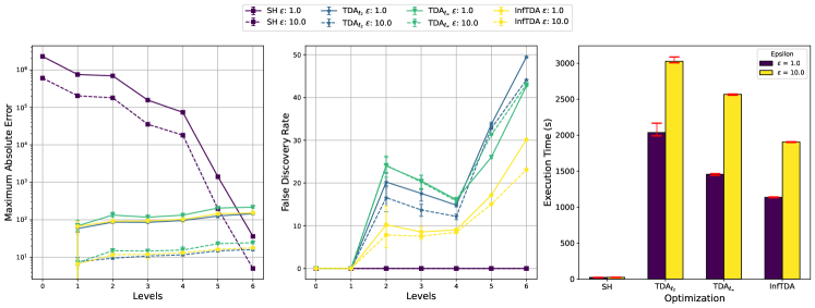
Figure 3. Experiments run for the Italy ISTAT dataset. From left to right: maximum absolute error, false discovery rate, and execution time. The error-bars indicate maximum and minimum value over 10 experiments.

This section provides an experimental evaluation of InfTDA against various baselines on both real world and synthetic datasets. We start by presenting the baselines used, then we introduce the datasets and the experimental setup.

Baselines

As simple baselines we use the injection of discrete Gaussian noise, and the application of the Stability-Based histogram, on the leaves’ attributes of the tree. They will be labeled respectively as VanillaGauss and SH. We are aware of more accurate baselines for sparse histogram (Desfontaines et al., 2022; Aumüller et al., 2021). However, in terms of maximum absolute error utility, they offer the same asymptotic performance as SH. VanillaGauss offers stronger guarantees for range queries compared to SH, but it is space-inefficient and can produce negative counts. Conversely, SH generates datasets with non-negative counts and no false positives; however, it performs poorly for range queries, particularly when the dataset consists predominantly of rare items. These baselines provide experimental evidence underscoring the necessity of using TopDown constraint optimization algorithms like TDA or our proposed InfTDA. We evaluate InfTDA against two variations of TopDown algorithms, each employing a different optimization strategy. The first, standard TDA, referred to as $\texttt{TDA}_{\ell_{2}}$, uses the Euclidean distance as the objective function. The second, denoted TDA${}_{\ell_{\infty}}$, incorporates Chebyshev optimization but relies on a black-box solver for the optimization process. This latter baseline allows us to assess the effectiveness of our optimizer, IntOpt, particularly in reducing false positives. We recognize the possibility of employing CBDP and the Hierarchical mechanism as a baselines. However, the first faces significant implementation obstacles due to the vast quantity of O/D pairs in the analyzed dataset, while the second does not work in the integer domain.

Real Dataset

The real world dataset under examination originates from the Italian National Institute of Statistics (ISTAT) (Istat, 2011), which encompasses data on commuting patterns between origins and destinations across Italy for the year 2011, delineated at the census section level, containing commuting information for 31.020.103 individuals. This dataset is structured with a geographical hierarchy of $5$ geo-partitions: regions, provinces, municipalities, section areas, and census sections, where the top of the hierarchy is represented by regions (i.e., larger areas). The first three geographical partitions are depicted in Figure 1. Given that the data on O/D flows is derived from commuting behaviors, the application of privacy measures through the substitution method, with a maximum contribution of one flow per user, is deemed appropriate. The dataset exhibits significant sparsity, containing 362.292 census sections which theoretically could result in over 100 billion possible O/D pairs; however, it only records 14.287.549 actual flows. Due to computational limitation, for our experiments we considered only O/D pairs up to the municipality level. Yet, this results in about $500$ thousands O/D pairs over more than $65$ million possible pairs. We generate the destination tree from this dataset, obtaining a tree of depth $T=6$.

Synthetic Datasets

We generate two types of synthetic geo-partitions, a binary partition and a random partition, to create six distinct O/D datasets. The binary geo-partition consists of 8 hierarchical levels, where each area is iteratively divided into two smaller areas, resulting in a binary destination tree with a depth of $T=16$. In contrast, the random geo-partition has 4 levels, where each area is randomly divided into $k$ smaller areas, with $k$ sampled uniformly from 2 to 10. This approach simulates real-world scenarios where areas are partitioned unevenly, creating a destination tree with variable structure. The O/D counts are sampled from a Pareto distribution ($\text{Pr}(x)\sim x^{-\beta}$, where $x$ represents the flow and $\beta>0$), a common pattern observed in mobility and social data (Han et al., 2011; Alessandretti et al., 2020). These counts are then assigned as attributes to the leaves of the generated trees. To evaluate the mechanisms under varying levels of sparsity, we simulate three scenarios: complete, where all leaves have positive attributes; dense, where $50\%$ of the leaves are assigned positives attributes; and sparse, where only $1\%$ of the leaves are assigned positives attributes. This allows for comprehensive testing of the mechanism’s performance across different sparsity conditions. The number of generated users, and the number of O/D in the synthetic dataset can be found in Table 1.

Dataset	Number of users	Number of O/D
Binary Complete	1051271	65536
Binary Dense	734688	32768
Binary Sparse	23302	655
Random Complete	2019580	189225
Random Dense	1003943	95612
Random Sparse	67840	1892

Table 1. Synthetic datasets info

Experimental Setup

The system was developed using open source libraries and Python 3.11. Our approach to differential privacy leveraged the OpenDP library (Gaboardi et al., 2020), which includes implementations of the discrete Gaussian mechanism and the Stability Histogram. For black-box optimizers, we utilized cvxpy (Agrawal et al., 2018; Diamond and Boyd, 2016). TDA${}_{\ell_{2}}$ first minimizes the Euclidean distance for the relaxed program in the real domain using CLARABEL (Chen and Goulart, 2023), then it performs a rounding and redistribute the exceeding in a similar fashion of InfTDA, hence by prioritizing the elimination of small values. TDA${}_{\ell_{\infty}}$ optimization works completely in the integer domain, and uses GLPK mixed integer optimizer. The tests were conducted using an Intel Xeon Processor W-2245 (8 cores, 3.9GHz), 128GB RAM and Ubuntu 20.04.3. The experiments and the code is freely available at the following link . Each mechanism is run $10$ times and the error-bars in the plots indicate the maximum and minimum value of the considered metric.

Privacy budget

The experiments were carried out with $\varepsilon\in[1,10]$ and $\delta=10^{-8}$ (sufficient to ensure that $\delta\ll 1/n$). Although we recognize that intelligent allocation of the privacy budget across levels can improve the utility of a differentially private dataset (as done in by the US Census (Bureau, 2020)), we opted for a uniform distribution of the budget across all levels. We used Lemma 3 to compute the privacy budget for zCDP.

Quality of the DP dataset

To assess the quality of the DP dataset $\tilde{D}$ we measured two key indicators that can be computed at any level of the tree: the maximum absolute error defined in Equation 2 and the false discovery rate, which is the percentage of O/D pairs present in $\tilde{D}$ but absent in the original data. In tree notation, for any level $\ell\in\{0,\dots,T\}$ the false discovery rate is

$$f_{d}(\ell;\tilde{D},D)=\frac{|\{u_{\ell}:\tilde{q}(u_{\ell})>0\wedge q(u_{\ell})=0\}|}{|\{u_{\ell}:\tilde{q}(u_{\ell})>0\}|}\cdot 100\%,$$

where $D$ is the original data.

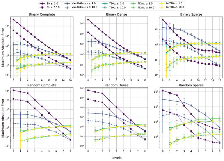
Figure 4. Experiments run for the synthetic datasets with focus on maximum absolute error. The error-bars indicate maximum and minimum value over 10 experiments

5.1. Discussion

Italian dataset

The analysis of the O/D commuting dataset for Italy is presented in Figure 3, which illustrates three metrics from left to right: the maximum absolute error per level, the false discovery rate per level, and the running time. We emphasize that the levels are defined as follows: the zero level represents the total number of users, the second level corresponds to range queries for regions, the fourth level pertains to provinces, and the final level corresponds to municipalities O/D pairs. The VanillaGauss method was not applied to this dataset due to the computational infeasibility of sampling more than 65 million Gaussian noises, one for each potential O/D pair. Instead, this baseline will be evaluated using synthetic data. We immediately observe that SH performs poorly on range queries, although it provides the most accurate estimates for O/D counts at finer geographical levels. Consistent with the theoretical results in Theorem 3, InfTDA produces datasets with diminishing accuracy as one moves down the levels of the tree, reflecting improved precision for O/D counts at larger geographical scales. This trend is similarly observed with TDA${}_{\ell_{2}}$ and TDA${}_{\ell_{\infty}}$. While TDA${}_{\ell_{2}}$ shows comparable utility to InfTDA, TDA${}_{\ell_{\infty}}$ underperforms slightly. This is due to the fact that Chebyshev optimization produces multiple optimal solutions, not all of which perform well in practice in terms of utility. This underscores the importance of our optimizer, IntOpt, in selecting the most practical solution. Notably, this is mainly observed in the middle plot in figure 3, on which we observe how InfTDA is able to significantly reduce the detection of false positives, in compare to TDA${}_{\ell_{\infty}}$ and TDA${}_{\ell_{2}}$. These observations hold for both high and low privacy budget. In terms of running time, SH is clearly the fastest as it does not need to perform any kind of optimization, and it runs linearly with the number of users $n$. InfTDA is the fastest TopDown algorithm. The running time increases with the privacy budget because, in the low-privacy regime, false negatives are more frequent. These occur when attributes that were positive in the sensitive dataset appear as zero in the DP dataset. This reduction in positive attributes typically decreases the size of the returned dataset, leading to fewer optimizations.

Synthetic Dataset

Figure 4 illustrates the maximum absolute error for the six synthetic datasets we generated. Unlike the previous analysis, this evaluation includes VanillaGauss. As expected, VanillaGauss demonstrates better accuracy than SH for range queries, particularly when the dataset is not highly sparse. Conversely, SH performs better on sparse datasets, though even in such cases, the error increases significantly for large range queries at the higher levels of the tree. The TopDown algorithms exhibit similar behavior across all scenarios, with an exception: TDA${\ell_{\infty}}$ over the random sparse dataset. While this deviation is not substantial compared to the other TDA algorithms, it provides valuable insights consistent with the findings from the Italy dataset. In trees with random branching factors, similar to the structure of the Italy tree, the number of variables in the optimization problem increases. This expansion of the solution space for the Chebyshev distance optimization raises the likelihood of sampling an optimal solution that performs poorly in practice. In contrast, this issue does not arise in binary trees, where each optimization involves only two variables, making it more likely to produce a unique solution for the Chebyshev minimization.

Figure 5 shows the false discovery rate for the sparse datasets. In the binary tree, no significant improvements are observed, indicating that when the optimization involves a small number of variables, the choice of the optimization function has minimal impact on the utility of the released datasets. In contrast, for the random tree, InfTDA produces a dataset with fewer false positives compared to the other mechanisms (with the obvious exception of SH).

Regarding the execution times of the algorithms, in Figure 6 it is clear how our optimizer is faster than a black-box optimizer. This is not only because of InfTDA returns a dataset with less false positives, as it runs faster even in the complete synthetic dataset.

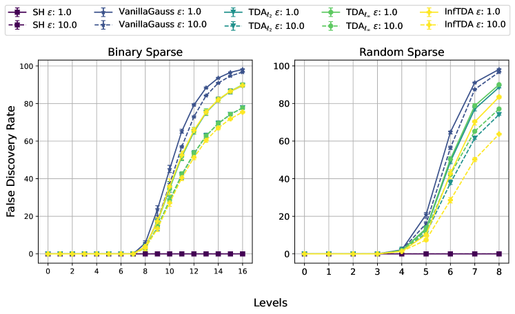
Figure 5. False discovery rate for synthetic datasets

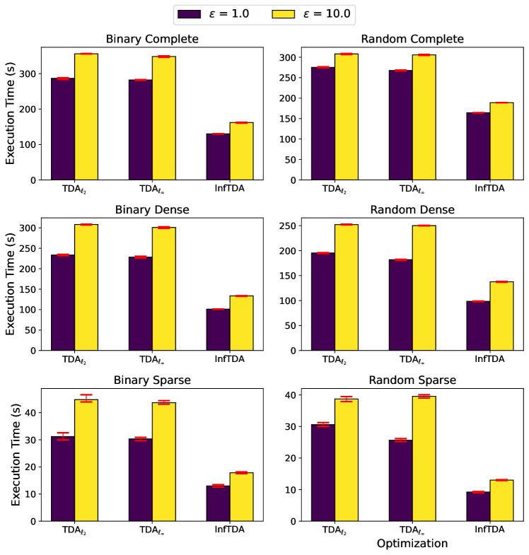
Figure 6. Running time for synthetic datasets and TDA

6. Conclusion and Future Directions

We found that a well-designed implementation of the TopDown algorithm can significantly improve accuracy in the differentially private release of O/D data with a hierarchical structure. This is particularly beneficial when producing tabular datasets where range queries must be more accurate for larger geographical areas. Specifically, this paper explores TopDown algorithms for general tree data structures with non-negative attributes and hierarchical consistency. We illustrate how any O/D dataset can be structured into the required tree format.

Additionally, we propose a Chebyshev distance constraint optimization problem as an alternative to the commonly used Euclidean distance minimization. This approach yields two key outcomes: a theoretical analysis of the maximum absolute error for a TopDown algorithm, and a practical, efficient integer optimization algorithm that effectively reduces false positives.

Our propose of TopDown algorithm InfTDA with our optimizer IntOpt, outperforms naive baselines and it is no worse than black-box implementation of TDA with different objective functions, on both real and synthetic datasets, while reducing effectively the false discovery rate.

Given the versatility of our approach, it would be valuable to test it on various real-world datasets beyond O/D data. Any tabular data, like healthcare data, can be used to construct a non-negative hierarchical tree, as long as a query hierarchy is defined. We leave this exploration for future research. In addition, we believe that a study of stability based algorithm as source of noise in a TDA would be interesting, especially in scenario where the hierarchy is made of unknown partitions. Finally, given the results of our experiments we believe that similar theoretical results hold for the TDA with Euclidean distance minimization.

Appendix A Additional Proof

Proof of Proposition 1.

We start by proving equation 4. By applying the discrete Gaussian mechanism on each attribute of the final level nodes we can reconstruct the attributes at any level using the hierarchical relation in equation 1. Consider a node $u_{\ell}$ at level $\ell\in\{0,\dots,T-1\}$, its private attribute is

$$\tilde{q}(u_{\ell})=\sum_{i_{\ell+1}\in\mathcal{C}(u_{\ell})}\dots\sum_{i_{T}\in\mathcal{C}(u_{T-1})}\tilde{q}(u_{T}),$$

so the error $\textnormal{err}(u_{\ell})=q(u_{\ell})-\tilde{q}(u_{\ell})$ is

(15) $$\textnormal{err}(u_{\ell})=\sum_{u_{\ell+1}\in\mathcal{C}(u_{\ell})}\dots\sum_{u_{T}\in\mathcal{C}(u_{T-1})}\big{[}q(u_{T})-\tilde{q}(u_{T})\big{]}.$$

Each error $q(u_{T})-\tilde{q}(u_{T})$ at the $T$ level is a Gaussian random variable $\mathcal{N}_{\mathbb{Z}}(0,1/\rho)$, then the right hand side of equation 15 is a Gaussian random variable $\mathcal{N}_{\mathbb{Z}}(0,b^{T-\ell}/\rho)$, as it is a summation of $b^{T-\ell}$ Gaussian random variables. Then, by applying Corollary 7 and a union bound over $b^{\ell}$ nodes, we obtain for $\beta\in(0,1)$

$$\text{Pr}\bigg{[}\max_{u_{\ell}\in V_{\ell}}|\textnormal{err}(u_{\ell})|\leq O\bigg{(}b^{\frac{T-\ell}{2}}\sqrt{\frac{\ell}{\rho}\log\bigg{(}\frac{b}{\beta}\bigg{)}}\bigg{)}\bigg{]}\geq 1-\beta.$$

We now prove equation 5. equation 15 is still applicable, however, the noise inserted at level $T$ follows a complicated distribution which is a result of a symmetric Laplace noise distribution followed by a truncation. So it is not straightforward to compute the distribution of composition of such random variables. Yet, we have that $|\textnormal{err}(u_{T})|\leq O\big{(}\frac{\log(1/\delta)}{\varepsilon}\big{)}$ with probability at least $1-\delta$. Therefore, by summing the error and applying a union bound over $n$, as we have at most $n$ random variables to sum, equation 15 leads to $|\textnormal{err}(u_{\ell})|\leq O\big{(}\min(b^{T-\ell},n)\frac{\log(1/\delta)}{\varepsilon}\big{)}$ with probability at least $1-n\delta$. As $\delta\ll 1/n$ it follows a constant probability upper bound. ∎

Appendix B Fast $\texttt{IntOpt}_{\infty}$

Algorithm 3 Polynomial time $\ell_{\infty}$ Integer Optimization (IntOpt_∞)

1:${\bf x}\in\mathbb{Z}^{b},c\in\mathbb{N}$.

2:${\bf z}\leftarrow\max\big{(}\big{\lceil}\frac{c-\sum_{i}x_{i}}{b}\big{\rceil},-{\bf x}\big{)}$

3:$t\leftarrow||\bf{z}||_{\infty}$

4:$I\leftarrow\text{sorted indices of ${\bf x}$}$

5:$I\leftarrow(i\in I:z_{i}>-x_{i})$

6:$i\leftarrow 0$

7:while $\sum_{i}z_{i}>c-\sum_{i}{x_{i}}$ do

8:  $\Delta\leftarrow\sum_{i}z_{i}-c+\sum_{i}x_{i}$

9:  $z_{I[i]}\leftarrow\max(z_{I[i]}-\Delta,-x_{I[i]},-t)$

10:  $i\leftarrow(i+1)\mod|I|$

11:  if $i=0$ then

12:   $I\leftarrow(i\in I:z_{i}>-x_{i})$

13:   $r\leftarrow\big{\lfloor}\frac{1}{|I|}\big{(}\sum_{i}z_{i}-c+\sum_{i}x_{i}\big{)}\big{\rfloor}$

14:   $t\leftarrow t+\max(1,r)$   

15:return ${\bf x}+{\bf z}$

This is the algorithm we implemented in our experiments. One key modification is that the while loop operates only on the indices of elements in $\mathbf{z}$ that can still be reduced, as specified in lines 4 and 11. The main modification is in line 12, where it is computed the smallest entry of $\bf z$ that, if $z_{i}=-t-r$ for any $i\in I$, then we would have

$$c-\sum_{i=1}^{d}x_{i}\leq\sum_{i=1}^{b}z_{i}\leq c-\sum_{i=1}^{b}x_{i}+|I|,$$

ensuring that only one additional reduction round is required to satisfy the equality constraint. If all elements are clipped to $-t-r$, the total summation decreases by $\sum_{i}z_{i}-r\cdot|I|$. The first inequality is derived as follows

$$\sum_{i=1}^{b}z_{i}-r\cdot|I| =\sum_{i=1}^{b}z_{i}-\bigg{\lfloor}\frac{1}{|I|}\big{(}\sum_{i}z_{i}-c+\sum_{i}x_{i}\big{)}\bigg{\rfloor}\cdot|I|$$

$$\geq\sum_{i=1}^{b}z_{i}-\frac{1}{|I|}\bigg{(}\sum_{i=1}^{b}z_{i}-c+\sum_{i=1}^{b}x_{i}\bigg{)}\cdot|I|=c-\sum_{i=1}^{b}x_{i},$$

while the second comes from

$$\sum_{i=1}^{b}z_{i}-r\cdot|I| \leq\sum_{i=1}^{b}z_{i}-\bigg{[}\frac{1}{|I|}\bigg{(}\sum_{i=1}^{b}z_{i}-c+\sum_{i=1}^{b}x_{i}\bigg{)}-1\bigg{]}\cdot|I|$$

$$=c-\sum_{i=1}^{b}x_{i}+|I|,$$

If not all elements are clipped to $-t-r$, at least one element is clipped to $-x_{i}$, reducing the cardinality of $I$ by at least 1. Consequently, after the first reduction loop (line 10), the algorithm either transitions to the second-to-last loop (where all elements are clipped to $-t-r$) or reduces $|I|$ to $|I|-1$. In the worst-case scenario, where $|I|=b$, it takes $O(b)$ iterations for $|I|$ to decrease by 1. Thus, the overall runtime of the algorithm is bounded by $O(b^{2})$.

References

- (1)
- Abowd et al. (2022) John M Abowd, Robert Ashmead, Ryan Cumings-Menon, Simson Garfinkel, Micah Heineck, Christine Heiss, Robert Johns, Daniel Kifer, Philip Leclerc, Ashwin Machanavajjhala, et al. 2022. The 2020 census disclosure avoidance system topdown algorithm. Harvard Data Science Review Special Issue 2 (2022).
- Agrawal et al. (2018) Akshay Agrawal, Robin Verschueren, Steven Diamond, and Stephen Boyd. 2018. A rewriting system for convex optimization problems. Journal of Control and Decision 5, 1 (2018), 42–60.
- Alessandretti et al. (2020) Laura Alessandretti, Ulf Aslak, and Sune Lehmann. 2020. The scales of human mobility. Nature 587, 7834 (2020), 402–407.
- Aumüller et al. (2021) Martin Aumüller, Christian Janos Lebeda, and Rasmus Pagh. 2021. Differentially private sparse vectors with low error, optimal space, and fast access. In Proceedings of the 2021 ACM SIGSAC Conference on Computer and Communications Security. 1223–1236.
- Balle and Wang (2018) Borja Balle and Yu-Xiang Wang. 2018. Improving the gaussian mechanism for differential privacy: Analytical calibration and optimal denoising. In International Conference on Machine Learning. PMLR, 394–403.
- Bun et al. (2019) Mark Bun, Kobbi Nissim, and Uri Stemmer. 2019. Simultaneous private learning of multiple concepts. Journal of Machine Learning Research 20, 94 (2019), 1–34.
- Bun and Steinke (2016) Mark Bun and Thomas Steinke. 2016. Concentrated differential privacy: Simplifications, extensions, and lower bounds. In Theory of Cryptography Conference. Springer, 635–658.
- Bureau (2020) U Bureau. 2020. Disclosure avoidance for the 2020 census: An introduction. (2020).
- Canonne et al. (2020) Clément L Canonne, Gautam Kamath, and Thomas Steinke. 2020. The discrete gaussian for differential privacy. Advances in Neural Information Processing Systems 33 (2020), 15676–15688.
- Chen and Goulart (2023) Yuwen Chen and Paul Goulart. 2023. An Efficient IPM Implementation for A Class of Nonsymmetric Cones. arXiv:2305.12275 [math.OC]
- Cormode et al. (2012) Graham Cormode, Cecilia Procopiuc, Divesh Srivastava, and Thanh TL Tran. 2012. Differentially private summaries for sparse data. In Proceedings of the 15th International Conference on Database Theory. 299–311.
- Cormode et al. (2011) Graham Cormode, Magda Procopiuc, Divesh Srivastava, and Thanh TL Tran. 2011. Differentially private publication of sparse data. arXiv preprint arXiv:1103.0825 (2011).
- Desfontaines et al. (2022) Damien Desfontaines, James Voss, Bryant Gipson, and Chinmoy Mandayam. 2022. Differentially private partition selection. Proceedings on Privacy Enhancing Technologies 1 (2022), 339–352.
- Diamond and Boyd (2016) Steven Diamond and Stephen Boyd. 2016. CVXPY: A Python-embedded modeling language for convex optimization. Journal of Machine Learning Research 17, 83 (2016), 1–5.
- Dwork (2006) Cynthia Dwork. 2006. Differential privacy. In International colloquium on automata, languages, and programming. Springer, 1–12.
- Dwork et al. (2006) Cynthia Dwork, Frank McSherry, Kobbi Nissim, and Adam Smith. 2006. Calibrating noise to sensitivity in private data analysis. In Theory of Cryptography: Third Theory of Cryptography Conference, TCC 2006, New York, NY, USA, March 4-7, 2006. Proceedings 3. Springer, 265–284.
- Dwork et al. (2014) Cynthia Dwork, Aaron Roth, et al. 2014. The algorithmic foundations of differential privacy. Foundations and Trends® in Theoretical Computer Science 9, 3–4 (2014), 211–407.
- Fioretto et al. (2018) Ferdinando Fioretto, Chansoo Lee, and Pascal Van Hentenryck. 2018. Constrained-based differential privacy for mobility services. In Proceedings of the 17th International Conference on Autonomous Agents and MultiAgent Systems. 1405–1413.
- Gaboardi et al. (2020) Marco Gaboardi, Michael Hay, and Salil Vadhan. 2020. A programming framework for opendp. Manuscript, May (2020).
- Gómez et al. (2019) Sergio Gómez, Alberto Fernández, Sandro Meloni, and Alex Arenas. 2019. Impact of origin-destination information in epidemic spreading. Scientific reports 9, 1 (2019), 2315.
- Han et al. (2011) Xiao-Pu Han, Qiang Hao, Bing-Hong Wang, and Tao Zhou. 2011. Origin of the scaling law in human mobility: Hierarchy of traffic systems. Physical Review E 83, 3 (2011), 036117.
- Hay et al. (2010) Michael Hay, Vibhor Rastogi, Gerome Miklau, and Dan Suciu. 2010. Boosting the accuracy of differentially private histograms through consistency. Proc. VLDB Endow. 3, 1–2 (sep 2010), 1021–1032. https://doi.org/10.14778/1920841.1920970
- Istat (2011) Istat. 2011. Matrici di contiguità, distanza e pendolarismo. https://www.istat.it/it/archivio/157423 Accessed: 2024-02-07.
- Korolova et al. (2009) Aleksandra Korolova, Krishnaram Kenthapadi, Nina Mishra, and Alexandros Ntoulas. 2009. Releasing search queries and clicks privately. In Proceedings of the 18th international conference on World wide web. 171–180.
- Lee et al. (2022) Inmook Lee, Shin-Hyung Cho, Kyoungtae Kim, Seung-Young Kho, and Dong-Kyu Kim. 2022. Travel pattern-based bus trip origin-destination estimation using smart card data. Plos one 17, 6 (2022), e0270346.
- Suresh (2019) Ananda Theertha Suresh. 2019. Differentially private anonymized histograms. Advances in Neural Information Processing Systems 32 (2019).
- Swanberg et al. (2023) Marika Swanberg, Damien Desfontaines, and Samuel Haney. 2023. DP-SIPS: A simpler, more scalable mechanism for differentially private partition selection. Proceedings on Privacy Enhancing Technologies 4 (2023), 257–268.
- Vadhan (2017) Salil Vadhan. 2017. The complexity of differential privacy. Tutorials on the Foundations of Cryptography: Dedicated to Oded Goldreich (2017), 347–450.
- Xu et al. (2013) Jia Xu, Zhenjie Zhang, Xiaokui Xiao, Yin Yang, Ge Yu, and Marianne Winslett. 2013. Differentially private histogram publication. The VLDB journal 22 (2013), 797–822.
- Zhang et al. (2014) Xiaojian Zhang, Rui Chen, Jianliang Xu, Xiaofeng Meng, and Yingtao Xie. 2014. Towards accurate histogram publication under differential privacy. In Proceedings of the 2014 SIAM international conference on data mining. SIAM, 587–595.