Traveling waves to a logarithmic chemotaxis model with fast diffusion and singularities 00footnotetext: *Corresponding author. 00footnotetext: E-mail addresses: lixw928@nenu.edu.cn (XL), dfli@hust.edu.cn (DL), lijy645@nenu.edu.cn (JL), ming.mei@mcgill.ca (MM).
Abstract: This paper is concerned with a chemotaxis model with logarithmic sensitivity and fast diffusion, which possesses strong singularities for the sensitivity at zero-concentration of chemical signal, and for the diffusion at zero-population of cells, respectively. The main purpose is to show the existence of traveling waves connecting the singular zero-end-state, and particularly, to show the asymptotic stability of these traveling waves. The challenge of the problem is the interaction of two kinds of singularities involved in the model: one is the logarithmic singularity of the sensitivity; and the other is the power-law singularity of the diffusivity. To overcome the singularities for the wave stability, some new techniques of weighted energy method are introduced artfully. Numerical simulations are also carried out, which further confirm our theoretical stability results, in particular, the numerical results indicate that the effect of fast diffusion to the structure of traveling waves is essential, which causes the traveling waves much steeper like shock waves. This new phenomenon is a first observation.
Keywords: Chemotaxis; fast diffusion; traveling waves; nonlinear stability; weighted energy estimates.
AMS (2020) Subject Classification: 35C07, 35B35, 35Q92, 92C17
1 Introduction
Models and Background. In this paper, we study the chemotaxis model [26, 28, 42, 51]
| (1.1) |
where is the population density of cells or bacteria, and is the concentration of chemical signal (e.g. nutrient). The cells diffuse nonlinearly in the form of , where denotes the diffusion exponent, which means the diffusion of cells is fast if , linear if or slow if . This nonlinear diffusion models the movement of cells in a porous medium or the mechanism of prevention of overcrowding for cells. The chemotactic response of the cells to the stimulation of the chemical signal is represented by , where represents the chemotactic coefficient that measures the strength of chemoattractants. Here the logarithmic sensitivity function comes from the pervasiveness of Weber-Fechner law, and was first introduced by Keller and Segel [26] to model the propagation of traveling band of bacteria observed in the celebrated experiment of Adler [1]. In the second equation, we neglect the diffusion of chemical signal because in many circumstances (e.g. Adler’s experiment [1]) the diffusion rate of typical signal is quite small compared to that of the cells. This model possesses two singularities: one is the singularity of sensitivity when , and the other is the singularity of fast diffusion for when .
When , the system (1.1) was proposed by Levine et al. [28] to model the initiation of tumor angiogenesis, where and denote the density of vascular endothelial cells and the concentration of vascular endothelial growth factor, respectively. In this biological process, the diffusion of endothelial growth factor is neglected since it is less important than its interaction with the endothelial cells. The mathematical derivation of this singular chemotaxis model has been obtained in Refs. [27] and [44] from the viewpoint of reinforced random walks. We also refer to Refs. [4] and [5] for the derivations of a variety of cross-diffusion models via the micro-macro asymptotic method.
Since the pioneering work of Keller and Segel [26], the analysis of traveling waves has become one of the most important research topics in chemotaxis, as many complex wave patterns have been observed in various experiments of chemotaxis [1, 18, 40, 46, 56]. For instance, E. coli in a capillary tube might move as a traveling band by consuming oxygen [1], Dictyostelium discoideum generated a spiral wave in seeking cyclic adenosine monophosphate [18], and myxobacteria migrated towards some chemical signal as a periodic traveling wave [56]. In mathematics, most of the achievements are concerned with the case of linear diffusion (i.e. ). See Ref. [54] for the first result on the existence of monotone traveling wave, Refs. [24, 32] for the stability of such traveling waves under appropriate perturbations, and Refs. [20, 35, 45] for the effect of logistic growth. When the chemical diffusion is considered in the second equation, the existence and stability of monotone traveling wave solutions were studied in Ref. [31]. For more analytical works on traveling waves of chemotaxis models with linear diffusion, we refer the interested readers to Ref. [53].
When , the system (1.1) models the chemotactic behaviors of cells or bacteria in porous media. The chemotaxis of cells and bacteria in porous media is important in both experiments and mathematics. Indeed, experiments were took in Refs. [42] and [51] to quantify the bacterial chemotaxis in porous media. To prevent overcrowding of bacteria, nonlinear diffusion for chemotaxis models was introduced in Refs. [8, 12, 17, 21]. Furthermore, Mendez et al. [39] derived mathematically the chemotaxis model with nonlinear diffusion from the viewpoint of Markovian reaction-random walks. There are also fruitful theoretical works on the chemotaxis model of self-aggregation type with nonlinear diffusion, where the chemical signal is generated by the cells. See Refs. [6, 11, 25, 47] for the uniqueness, extinction behavior, blowup problem and stationary distributions of the solutions if the diffusion of cells is fast, Refs. [49, 50] for the global boundedness of solutions, and Refs. [3, 6, 7, 13] for the colorful dynamics of the system if the diffusion of cells is slow. We refer to Ref. [10] for a systematical review of literatures in this direction.
If the chemotaxis model with nonlinear diffusion is of consumption type, like (1.1), the understanding of its dynamics is quite limited. For the slow diffusion case, Yan and Li [59] constructed a global generalized solution to the system (1.1) on a bounded domain with Neumann boundary condition, and Jin [23] showed the existence of global weak solutions for large initial data and proved the stability of constant steady states to a chemotaxis-consumption model with linear sensitivity. Regarding the traveling waves, Kim and his collaborators [15, 16] are the first to construct compactly supported traveling waves to (1.1) in the slow diffusion region (i.e. ), while the problem of stability of such waves was left open due to the strong degeneracy of slow diffusion. Very recently, Refs. [2, 9] have constructed a series of exotic traveling waves that may be regular, singular and even discontinuous for the porous-media flux-saturated chemotaxis models, while the stability of these traveling waves are unknown. The purpose of this paper is to deal with the much less understood case of fast diffusion (i.e. ). We shall show both the existence and stability of traveling waves in the fast diffusion case.
Traveling waves and singularities. Before introducing the challenges of this problem, we present some elementary properties of the traveling waves. Here we mean the traveling wave of system (1.1) is a non-constant smooth self-similar solution in the form of
satisfying
| (1.2) |
where , is called the moving coordinate and is the wave speed. Substituting this wave ansatz into the system (1.1) yields the equations of
| (1.3) |
Notice that by (1.2) and the second equation of (1.3), it holds that
| (1.4) |
On the other hand, thanks to , and , we get from the second equation of (1.3) that . This implies that . Hence, by (1.4), we have and subsequently . Utilizing (1.4) again, it gives . Then the following properties of can be verified:
| (1.5) |
Therefore, to investigate the stability of traveling waves to (1.1), it is necessary to equip (1.1) with the following initial conditions
| (1.6) |
One can observe from the fact that, the system (1.1) with has two types of singularities: one is the singular sensitivity at the constant-state , and the other is the singular diffusivity at the constant-state .
In this paper, we shall exploit some novel strategies to overcome the analytical difficulties generated by the interaction of the two singularities. As in the arguments of Refs. [24, 32, 34], we take the following Hopf-Cole transformation
| (1.7) |
to remove the singular logarithmic sensitivity. Then we transfer the system (1.1) with (1.6) into the following parabolic-hyperbolic system
| (1.8) |
with initial data
| (1.9) |
where
Now the primary obstacle is the singular diffusivity since . In addition, the nonlinear diffusion results in undesirable tedious estimates. In this paper, we shall develop some new ideas to establish the existence and stability of traveling waves to the system (1.1) with . Specifically, we are going to show that:
- (i)
-
(ii)
the traveling wave obtained above is nonlinearly asymptotically stable in some topological space (see Theorem 2.4).
The stability of traveling waves with fast diffusions and the singular state is also numerically demonstrated in different cases. Remarkably, the numerical simulations show that the stronger fast diffusion causes the shape of traveling waves to be more steeper like shock waves, and the oscillations slowly disappear. This means that the effect of fast diffusion with the singular state is essential for the structure of traveling waves. This new phenomenon is a first observation.
Strategies for treating singularities. To prove the result (i), we first establish the existence of monotone traveling wave solution to transformed system (1.8)-(1.9). Based on the conservation structure of this system, it is easy to see that satisfies a first-order ordinary differential equation that can be easily resolved. Then we define the wave component through the second equation of (1.3). Therefore, the existence of traveling waves to the system (1.1) can be obtained without too much analytical effort. In order to show the result (ii), it is natural to study the asymptotic stability of to the system (1.8)-(1.9) first. However, we still need to deal with the challenge of the singularity of since and . To settle this difficulty, we first employ the technique of taking anti-derivatives to classify the strength of the singularity. Then according to the structure of the fast diffusion, we take a weighted functional space to control the singularity where the weights are carefully constructed. In particular, we have to select a piecewise smooth weight function in the basic estimate. Furthermore, in the and estimates, the interaction of the singular diffusivity and weighted functional space results in an unfavorable obstacle that, non-zero boundary terms may arise in the integration by parts. We break down this obstacle by introducing a regular approximate weight function that removes part of the singularity. After establishing uniform estimates that are independent of the artificial parameter, we obtain the desired energy estimates by using the Fatou’s Lemma. To our knowledge, this is the first analytical work on the nonlinear stability of traveling waves to the partial differential equations (PDE) with fast diffusion. The approach based on weighted energy estimates is flexible and is expected to be useful for the study of stability of wave patterns to other more sophisticated PDE models.
Before concluding this section, we recall some related works on the transformed system (1.8) with . In the one-dimensional case, the nonlinear stability of traveling waves was first obtained by Li and Wang [34] under appropriate perturbations if the waves are away from zero. Especially, the authors discovered a cancellation structure in the energy estimate that was quite helpful in the following studies. Recently, Choi et al. [14] proved the orbital stability of traveling waves to (1.8) with under general perturbations. The global existence of large solutions for the Cauchy problem and the initial-boundary value problem were carried out in Refs. [19, 30] and [38, 60], respectively. In the multidimensional case, the global existence of small solutions to the Cauchy problem and the initial-boundary value problem were studied in Refs. [29, 52] and [33, 43], respectively. When the chemical diffusion is included in the second equation, we refer to Refs. [22, 55, 57, 58] for various interesting works.
The rest of this paper is organized as follows. In section 2, we state our main results on the existence and nonlinear stability of traveling wave solutions to the parabolic-hyperbolic system (1.8) and the original chemotaxis system (1.1), respectively. Section 3 is devoted to the proof of the existence of traveling waves. In section 4, we first show the nonlinear stability of traveling waves to the system (1.8) on the basis of weighted energy estimates, and then transfer the stability result back to the original chemotaxis model (1.1). In section 5, we present some numerical simulations in different cases, which further perfectly confirm our theoretical results of wave stability.
2 Preliminaries and main results
By using the Hopf-Cole transformation (1.7), the chemotaxis system (1.1) is transformed into the parabolic-hyperbolic system (1.8), in which the logarithmic singularity of the sensitive function is removed. In the following we shall first study the existence and nonlinear stability of traveling wave solutions to the transformed system (1.8)-(1.9), and then transfer the results back to the original chemotaxis system.
The traveling wave solution of (1.8)-(1.9) is a non-constant self-similar solution given by
| (2.1) |
Substituting this wave ansatz into (1.8), we get the following equations of
| (2.2) |
From (1.5) and (1.7), one can easily see that
Hence, the boundary conditions of (2.2) read
| (2.3) |
It is expected that . Then integrating (2.2) over yields the Rankine-Hugoniot condition
| (2.4) |
which further gives
| (2.5) |
Theorem 2.1.
Remark 2.1.
The wave component decays at an algebraic rate as . This is in contrast to the case of linear diffusion where the waves decay to at an exponential rate as (see Refs. [24] and [32]). This phenomenon also verifies the principle that the range is usually referred to as “fast diffusion”, in the sense that the faster diffusion (than linear diffusion) occurs for small values of the density.
We next investigate the stability of the traveling wave solution to the transformed system (1.8)-(1.9). One may observe that this new system still has a strong singularity in the diffusivity since , which leads to a challenging problem. In this paper, we shall develop some novel ideas to resolve this strong singularity.
To state our result more precisely, we introduce some notation. The integrals and will be abbreviated as and , respectively. is the usual -th order Sobolev space with norm . denotes the weighted space of measurable functions so that for with norm . For simplicity, we denote , , and .
The nonlinear stability of the traveling wave solution to transformed system (1.8)-(1.9) is stated as follows.
Theorem 2.2.
Let be the traveling wave solution obtained in Theorem 2.1. Assume that there exists a constant such that where
Then there exists a positive constant such that if , then the Cauchy problem (1.8)-(1.9) admits a unique global solution satisfying
| (2.8) |
where the weight functions , , are defined by
| (2.9) |
with
Furthermore, the solution has the following asymptotic convergence
| (2.10) |
By using the Hopf-Cole transformation (1.7), we transfer the results of Theorems 2.1 and 2.2 back to the original chemotaxis model (1.1).
Theorem 2.3 (Existence of traveling waves).
3 Existence of traveling waves
In this section, we first prove the existence of monotone traveling wave solution to the system (2.2)-(2.3). After that, we define the wave component through the second equation of (1.3) which yields the traveling wave solutions to the original chemotaxis system (1.1).
Proof of Theorem 2.1.
Integrating (2.2) over , by (2.3), we have
| (3.1) |
which can be simplified to an ordinary differential equation (ODE) as
| (3.2) |
When satisfies (2.4), by (2.5) one can see that
| (3.3) |
Set . Noting for all , we only need to find the global solution of the following ODE
| (3.4) |
which is equivalent to
| (3.5) |
Integrating (3.5) gives
Clearly, for any given , the function is monotonically decreasing. Moreover, since , in view of (3.3), we get
Therefore, there exists a unique continuous function such that
Using this , one can define through the second equation of (3.1). The monotonicity of follows from (3.3)-(3.4) and the second equation of (3.1).
We next investigate the convergence rates of as . Since as , according to the asymptotic theory of ODE, the convergence rate of solutions to (3.4) as is determined by the equation
By a direct calculation, we get
which indicates that
On the other hand, the convergence rate of as is determined by
It is easy to see that
Hence
The proof is complete. ∎
Remark 3.1.
Since , it is easy to see from (3.4) that
| (3.6) |
Proof of Theorem 2.3.
4 Nonlinear stability
In this section, we first study the nonlinear stability of the traveling wave solution for the parabolic-hyperbolic system (1.8)-(1.9). And then by using the Hopf-Cole transformation (1.7), we prove the nonlinear stability of the traveling wave solution for the original chemotaxis system (1.1).
4.1 Reformulation of the problem
Let be the traveling wave obtained in Theorem 2.1. We write the system (1.8) without viscosity in the form
where
Denote by the first eigenvector of Jacobian matrix . Then according to the theory of hyperbolic conservation laws, [48] the vectors and are linearly independent. Thus there are two numbers and such that
provided that and are integrable over . Thanks to the work of Liu and Zeng on the stability of viscous shock waves, [36, 37] the coefficient may generate diffusion waves for small-amplitude viscous shock waves. In this paper, we aim to show the stability of large-amplitude traveling waves and, for simplicity, consider the case . We leave the case for future study. Now by the conservation laws, we have
| (4.1) | ||||
We thus employ the anti-derivative technique to study the asymptotic stability of traveling wave . Decompose the solution of (1.8) as
| (4.2) |
where . That is
| (4.3) |
for all and . It then follows from (4.1) that
| (4.4) |
Without loss of generality, we assume that the translation , which implies the initial perturbation is of zero mass
Now substituting (4.2) into (1.8), integrating the system over , and using (2.2) and (4.4), we derive the equation of :
| (4.5) |
where , and the initial condition is given by
| (4.6) |
with . One may observe that the perturbation system (4.5) has a singular diffusivity near since and , in the sequel we shall carefully select weighted functional space to resolve the singularity.
4.2 Energy estimates
We search for the solutions of (4.5)-(4.6) in the following space
where the weight functions , , are defined by
| (4.7) |
with
Denote
| (4.8) |
Then we have the following global well-posedness result for the Cauchy problem (4.5)-(4.6).
Proposition 4.1.
The local well-posedness of the system (4.5)-(4.6) is standard (see Ref. [41] for instance). To prove Proposition 4.1, we only need to establish the following a priori estimate.
Proposition 4.2 (A priori estimate).
Before establishing the a priori estimate in Proposition 4.2, we first present some preliminary calculations.
Lemma 4.1.
Let be the traveling wave obtained in Theorem 2.1. Denote for some positive constant , then it holds
| (4.10) |
where is a positive constant independent of .
Proof.
By the weighted Sobolev inequality (4.10), it is easy to see that
| (4.12) |
Lemma 4.2.
Proof.
We now derive the basic estimate of .
Lemma 4.3.
Let the assumptions of Proposition 4.2 hold. If , then there exists a constant independent of such that
| (4.16) |
for any .
Proof.
Denote by a smooth positive weight function. Multiplying the first equation of (4.5) by and the second one by , adding them and integrating by parts, noting that
and
we obtain
| (4.17) | ||||
By the Cauchy-Schwarz inequality, the last term on the right hand side of (4.17) satisfies
where is a positive constant to be determined later. It thus follows from (4.17) that
| (4.18) |
where
We next determine the weight function and the constant so that and for all . To ensure , given that according to (2.6), we may take
| (4.19) |
where is a constant to be determined later. Given this, by (3.1)-(3.2), one can see that
| (4.20) |
Now we take
| (4.21) |
so that . Therefore, by virtue of , (2.6) and (4.20), we get
| (4.22) |
On the other hand, utilizing (4.13), we can estimate the last term on the right-hand side of (4.18) after integration by parts as
| (4.23) |
Thanks to (3.6) and (4.19), along with the fact that , it holds that
| (4.24) |
due to . Now inserting (4.22)-(4.24) into (4.18) yields
| (4.25) |
where
| (4.26) |
We claim that
| (4.27) |
In fact, when , we have due to (4.21). And then the two eigenvalues of satisfies . Therefore, is positive definite and the claim is true for . When , thanks to (4.21), we have from (4.27) that for any . Hence in any case, (4.27) is true, which along with (4.26) gives rise to
| (4.28) |
Substituting (4.28) into (4.25), we then arrive at
| (4.29) |
Noting , by the Cauchy-Schwarz inequality, we have
| (4.30) |
And the last term on the right hand side of (4.29) can be estimated as
| (4.31) |
where we have used . Combining (4.30) and (4.31), after choosing suitably small, we thus update (4.29) as
| (4.32) |
Then integrating (4.32) over gives the desired estimate (4.16). ∎
The next lemma gives the estimate of . An issue in the weighted energy estimates for higher order derivatives is that the singularity caused by fast diffusion may generate non-zero boundary terms during the integration by parts. To break down this barrier, we develop an approximate procedure that avoids the boundary terms after integration by parts, and obtain the desired weighted estimates by employing the Fatou’s Lemma.
Lemma 4.4.
Let the assumptions of Proposition 4.2 hold. If , then it holds
| (4.33) |
Proof.
Differentiating (4.5) with respect to yields
| (4.34) |
Denote , where is a constant. Multiplying the first equation of (4.34) by and the second one by , integrating the resultant equations with respect to , noting
and
we get
| (4.35) |
Next, we estimate the terms on the right hand side of (4.35). Noting and , by (3.6) and the Cauchy-Schwarz inequality, we deduce that
| (4.36) |
Similarly, by the second equation of (2.2), we have
| (4.37) |
and
| (4.38) |
In view of (3.6) and the fact that , by integration by parts, we get
| (4.39) | ||||
and by (4.14), the last term on the right hand side of (4.35) can be estimated as
| (4.40) |
Substituting (4.36)–(4.40) into (4.35) and integrating the equation with respect to , noting , and , we have
provided that is small enough. Moreover, it follows from the Fatou’s Lemma that
| (4.41) |
Next, we claim
| (4.42) |
To prove (4.42), we multiply the first equation of (4.5) by to get
| (4.43) |
Noting that by the second equation of (4.34), it holds
Integrating (4.43) over , we obtain
| (4.44) |
where, in view of (3.6) and the Taylor’s expansion, it holds that
We thus have from (4.44) that
where we have used the fact and . This along with (4.16) and (4.41) gives rise to (4.42), provided that is small enough.
To close the a priori estimate, we further need the estimate of the second order derivative of .
Lemma 4.5.
Let the assumptions of Proposition 4.2 hold. Then it holds for any ,
| (4.47) |
Proof.
We differentiate (4.34) with respect to to get
| (4.48) |
Multiplying the first equation of (4.48) by and the second one by , we obtain
| (4.49) |
By (3.6) and the Cauchy-Schwarz inequality, we have
| (4.50) |
and
| (4.51) |
Notice that (3.2) gives
| (4.52) |
which in combination with (3.6) implies that
| (4.53) |
Owing to the second equation of (2.2), it holds
| (4.54) |
On the other hand, (4.52) also gives
| (4.55) |
Now by (3.6) and (4.53), we get
| (4.56) |
By (2.2), (4.54) and the fact that , we have
| (4.57) |
where we have used in the second inequality. Noting and , thanks to (3.6), one obtains
| (4.58) |
The sixth term on the right hand side of (4.49) can be estimated as follows. After integration by parts, we get
where, by virtue of (3.6) and the Cauchy-Schwarz inequality, it holds that
and
Thanks to (4.55) and (3.6), we have
and
Thus, noting , we have
| (4.59) |
We next estimate the last term on the right hand side of (4.49). By (4.15), we get
By (3.6), and Hölder’s inequality, we derive
where we have used in the second inequality that due to . And thanks to (3.6) and , it holds that
where we have used the fact in the last inequality. Thus,
| (4.60) |
Now substituting (4.50)-(4.60) into (4.49), and integrating the inequality with respect to , by Lemma 4.4, we obtain
| (4.61) |
provided that is suitably small. Letting , by Fatou’s Lemma, it then follows that
| (4.62) |
Next we estimate . Multiplying the first equation of (4.34) by , we get
Noting that
we have
| (4.63) |
where,
| (4.64) |
By Taylor’s expansion, and Hölder’s inequality, we deduce that the first term on the right hand side of (4.64) satisfies
| (4.65) |
Utilizing (3.6), (4.53) and the Cauchy-Schwarz inequality, we have
| the other terms of (4.64) | |||
| (4.66) |
Moreover, since and , by (3.6), we get
| (4.67) |
The last term on the right hand side of (4.63) can be estimated as
| (4.68) |
where we have used and . Because and , adding (4.64)-(4.68) with (4.63) and utilizing (4.33) and (4.62), we then arrive at
| (4.69) |
Combining (4.62) and (4.69) and following the same procedure as in (4.45), we obtain (4.47) provided that is small enough. Thus, the proof of Lemma 4.5 is finished. ∎
4.3 Proof of main results
Proof of Theorem 2.2.
The a priori estimate (4.9) guarantees that is small for all if is small enough. Hence applying the standard extension procedure, we obtain the global well-posedness of the system (4.5)-(4.6) in . Thanks to the decomposition (4.2), the system (1.8)-(1.9) has a unique global solution satisfying (2.8). It remains to show the convergence (2.10). In view of (4.2) again, it suffices to show
| (4.70) |
where . We denote . By the estimate (4.9), we have
which implies . We next show that . By the equation (4.34), and using , we have
and
Thus,
It then follows that
Now for all , we get
where we have used the boundedness of . Hence
Applying the same procedure to leads to
Therefore (4.70) is proved and the proof of Theorem 2.2 is complete. ∎
Proof of Theorem 2.4.
Owing to (4.2) and the Hopf-Cole transformation (1.7), we have
which gives
Then it is easy to see that the assumption of Theorem 2.4 verifies that of Theorem 2.2. Hence according to Theorem 2.2, the transformed problem (1.8)-(1.9) admits a unique global solution satisfying the regularity (2.8) and the asymptotic convergence (2.10).
We next show the desired results of . By the second equation of (1.1), one can solve as
which, in combination with the fact that , leads to
| (4.71) |
Now by (4.2) and the transformation (1.7) again, one deduces that
Hence
By Taylor’s expansion, we have
| (4.72) |
By Proposition 4.1, one can see that is small. Thus, we conclude that the series is absolutely convergent in . This together with the regularities of and implies
It remains to show the asymptotic convergence of . Thanks to (4.71)-(4.72) and the convergence of , we have
The proof is complete. ∎
5 Numerical simulations
In this section, we are going to present some numerical simulations in three cases for the equations
| (5.1) |
with and , and the following initial data
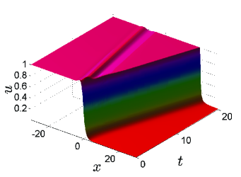
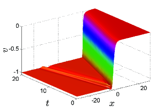
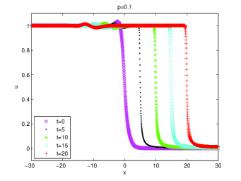
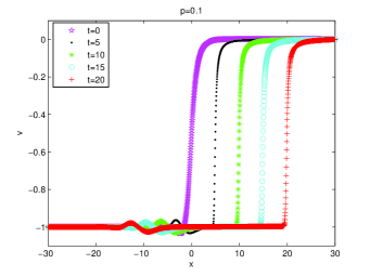
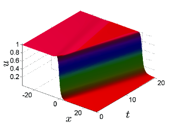
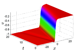
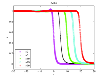
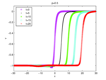
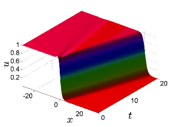
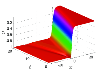
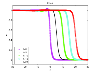
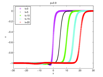

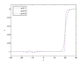
To numerically solve the problem conveniently, we set the computational domain and consider problem (5.1) with homogeneous Neumann boundary conditions. Then, the spatial discretization is done by the second-order central finite different methods with stepsize . And the time discretization is done by the Crank-Nicolson method with the stepsize . The fully-discrete schemes give a system of nonlinear equations, which is solved by Newton iterative method with the iterative residual . The numerical results with different parameters are shown in Figures 1-6, respectively. It can be seen from the figures that the numerical solutions of and behave like two traveling waves. The larger the parameter is, the more obvious dissipative effect can be found. All the numerical results indicate that the traveling wave solutions are stable as time increases. They confirm the theoretical results in this paper. In particular, from Figure 7, we see that the stronger fast diffusion (the smaller value of ) makes the traveling waves much steeper like shock waves, namely, the effect of fast diffusion with the singular state to the structure of traveling waves is essential.
6 Acknowledgements
The research of D. Li is supported by the National Natural Science Foundation of China (Nos. 11771162, 12231003). The research of J. Li is supported by the Natural Science Foundation of Jilin Province (No. 20210101144JC) and the National Natural Science Foundation of China (No. 12371216). The research of M. Mei is supported in part by NSERC grant RGPIN 2022-03374.
References
- [1] J. Adler, Chemotaxis in bacteria, Science, 153 (1966), 708–716.
- [2] M. Arias, J. Campos and J. Soler, Cross-diffusion and traveling waves in porous-media flux-saturated Keller-Segel models, Math. Models Methods Appl. Sci., 28 (2018), 2103–2129.
- [3] J. Bedrossian, N. Rodríguez and A. L. Bertozzi, Local and global well-posedness for aggregation equations and Patlak-Keller-Segel models with degenerate diffusion, Nonlinearity, 24 (2011), 1683–1714.
- [4] N. Bellomo, A. Bellouquid, Y. Tao and M. Winkler, Toward a mathematical theory of Keller-Segel models of pattern formation in biological tissues, Math. Models Methods Appl. Sci., 25 (2015), 1663–1763.
- [5] N. Bellomo, N. Outada, J. Soler, Y. Tao and M. Winkler, Chemotaxis and cross-diffusion models in complex environments: Models and analytic problems toward a multiscale vision, Math. Models Methods Appl. Sci., 32 (2022), 713–792.
- [6] S. Bian and J. Liu, Dynamic and steady states for multi-dimensional Keller-Segel model with diffusion exponent , Commun. Math. Phys., 323 (2013), 1017–1070.
- [7] A. Blanchet, J. A. Carrillo and P. Laurençot, Critical mass for a Patlak-Keller-Segel model with degenerate diffusion in higher dimensions, Calc. Var. Partial Differ. Equ., 35 (2009), 133–168.
- [8] M. Burger, M. Di Francesco and Y. Dolak-Strub, The Keller-Segel model for chemotaxis with prevention of overcrowding: linear vs. nonlinear diffusion, SIAM J. Math. Anal., 38 (2006), 1288–1315.
- [9] J. Campos, C. Pulido, J. Soler and M. Veruete, Singular patterns in Keller-Segel-type models, Math. Models Methods Appl. Sci., 33 (2023), 1693–1719.
- [10] J. A. Carrillo, K. Craig and Y. Yao, Aggregation-diffusion equations: dynamics, asymptotics, and singular limits, Springer International Publishing, New York, 2019, pp. 65–108.
- [11] J. A. Carrillo, M. G. Delgadino, R. L. Frank and M. Lewin, Fast Diffusion leads to partial mass concentration in Keller-Segel type stationary solutions, Math. Models Methods Appl. Sci., 32 (2022), 831–850.
- [12] J. A. Carrillo, S. Hittmeir and A. Jüngel, Cross diffusion and nonlinear diffusion preventing blow up in the Keller-Segel model, Math. Models Methods Appl. Sci., 22 (2012), 1250041, 35 pp.
- [13] L. Chen, J. Liu and J. Wang, Multidimensional degenerate Keller-Segel system with critical diffusion exponent , SIAM J. Math. Anal., 44 (2012), 1077–1102.
- [14] K. Choi, M.-J. Kang, Y.-S. Kwon and A. F. Vasseur, Contraction for large perturbations of traveling waves in a hyperbolic-parabolic system arising from a chemotaxis model, Math. Models Methods Appl. Sci., 30 (2020), 387–437.
- [15] S.-H. Choi and Y.-J. Kim, Chemotactic traveling waves by metric of food, SIAM J. Appl. Math., 75 (2015), 2268–2289.
- [16] S.-H. Choi and Y.-J. Kim, Chemotactic traveling waves with compact support, J. Math. Anal. Appl., 488 (2020), 124090, 21 pp.
- [17] Y.-S. Choi and Z.-A. Wang, Prevention of blow-up by fast diffusion in chemotaxis, J. Math. Anal. Appl., 362 (2010), 553–564.
- [18] R. E. Goldstein, Traveling-wave chemotaxis, Phys. Rev. Lett., 77 (1996), 775–778.
- [19] J. Guo, J. Xiao, H. Zhao and C. Zhu, Global solutions to a hyperbolic-parabolic coupled system with large initial data, Acta Math. Sci., 29 (2009), 629–641.
- [20] C. Henderson, Slow and fast minimal speed traveling waves of the FKPP equation with chemotaxis, J. Math. Pures Appl., 167 (2022), 175–203.
- [21] T. Hillen and K. Painter, Global existence for a parabolic chemotaxis model with prevention of overcrowding, Adv. Appl. Math., 26 (2001), 280–301.
- [22] Q. Hou, C.-J. Liu, Y.-G. Wang and Z. Wang, Stability of boundary layers for a viscous hyperbolic system arising from chemotaxis: one dimensional case, SIAM J. Math. Anal., 50 (2018), 3058–3091.
- [23] C. Jin, Large time behavior of solutions to a chemotaxis model with porous medium diffusion, J. Math. Anal. Appl., 478 (2019), 195–211.
- [24] H.-Y. Jin, J. Li and Z.-A. Wang, Asymptotic stability of traveling waves of a chemotaxis model with singular sensitivity, J. Differ. Equ., 255 (2013), 193–219.
- [25] T. Kawakami and Y. Sugiyama, Uniqueness theorem on weak solutions to the Keller-Segel system of degenerate and singular types, J. Differ. Equ., 260 (2016), 4683–4716.
- [26] E. F. Keller and L. A. Segel, Traveling bands of chemotactic bacteria: a theoretical analysis, J. Theor. Biol., 30 (1971), 235–248.
- [27] H. A. Levine and B. D. Sleeman, A system of reaction diffusion equations arising in the theory of reinforced random walks, SIAM J. Appl. Math., 57 (1997), 683–730.
- [28] H. A. Levine, B. D. Sleeman and M. Nilsen-Hamilton, A mathematical model for the roles of pericytes and macrophages in the initiation of angiogenesis. I. The role of protease inhibitors in preventing angiogenesis, Math. Biosci., 168 (2000), 77–115.
- [29] D. Li, T. Li and K. Zhao, On a hyperbolic-parabolic system modeling chemotaxis, Math. Models Methods Appl. Sci., 21 (2011), 1631–1650.
- [30] D. Li, R. Pan and K. Zhao, Quantitative decay of a one-dimensional hybrid chemotaxis model with large data, Nonlinearity, 7 (2015), 2181–2210.
- [31] J. Li, T. Li and Z.-A. Wang, Stability of traveling waves of the Keller-Segel system with logarithmic sensitivity, Math. Models Methods Appl. Sci., 24 (2014), 2819–2849.
- [32] J. Li and Z. Wang, Convergence to traveling waves of a singular PDE-ODE hybrid chemotaxis system in the half space, J. Differ. Equ., 268 (2020), 6940–6970.
- [33] T. Li, R. Pan and K. Zhao, Global dynamics of a hyperbolic-parabolic model arising from chemotaxis, SIAM J. Appl. Math., 72 (2012), 417–443.
- [34] T. Li and Z.-A. Wang, Nonlinear stability of traveling waves to a hyperbolic-parabolic system modeling chemotaxis, SIAM J. Appl. Math., 70 (2009), 1522–1541.
- [35] T. Li and Z.-A. Wang, Traveling wave solutions of a singular Keller-Segel system with logistic source, Math. Biosci. Eng., 19 (2022), 8107–8131.
- [36] T.-P. Liu and Y. Zeng, Time-asymptotic behavior of wave propagation around a viscous shock profile, Commun. Math. Phys., 290 (2009), 23–82.
- [37] T.-P. Liu and Y. Zeng, Shock waves in conservation laws with physical viscosity, Mem. Amer. Math. Soc., 2015.
- [38] V. R. Martinez, Z.-A. Wang and K. Zhao, Asymptotic and viscous stability of large-amplitude solutions of a hyperbolic system arising from biology, Indiana Univ. Math. J., 67 (2018), 1383–1424.
- [39] V. Mendez, D. Campos, I. Pagonabarraga and S. Fedotov, Density-dependent dispersal and population aggregation patterns, J. Theor. Biol., 309 (2012), 113–120.
- [40] A. V. Narla, J. Cremer, and T. Hwa, A traveling-wave solution for bacterial chemotaxis with growth, Proc. Natl. Acad. Sci., 118 (2021), e2105138118, 12 pp.
- [41] T. Nishida, Nonlinear Hyperbolic Equations and Related Topics in Fluid Dynamics, Publ. Math. d’Orsay, 1978.
- [42] M. S. Olson, R. M. Ford, J. A. Smith and E. J. Fernandez, Quantification of bacterial chemotaxis in porous media using magnetic resonance imaging, Environ. Sci. Technol., 38 (2004), 3864–3870.
- [43] L. G. Rebholz, D. Wang, Z. Wang, C. Zerfas and K. Zhao, Initial boundary value problems for a system of parabolic conservation laws arising from chemotaxis in multi-dimensions, Disc. Cont. Dyn. Syst. Ser. A, 39 (2019), 3789–3838.
- [44] A. Stevens and H. G. Othmer, Aggregation, blowup, and collapse: The ABC’s of taxis in reinforced random walks, SIAM J. Appl. Math., 57 (1997), 1044–1081.
- [45] R. B. Salako and W. Shen, Spreading speeds and traveling waves of a parabolic-elliptic chemotaxis system with logistic source on , Disc. Cont. Dyn. Syst. Ser. A, 37 (2017), 6189–6225.
- [46] J. Saragosti, et al., Directional persistence of chemotactic bacteria in a traveling concentration wave, Proc. Natl. Acad. Sci., 108 (2011), 16235–16240.
- [47] Y. Sugiyama and Y. Yahagi, Extinction, decay and blow-up for Keller-Segel systems of fast diffusion type, J. Differ. Equ., 250 (2011), 3047–3087.
- [48] J. Smoller, Shock Waves and Reaction-Diffusion Equations, Springer-Verlag, Berlin, 1994.
- [49] Y. Tao and M. Winkler, Global existence and boundedness in a Keller-Segel-Stokes model with arbitrary porous medium diffusion, Discrete Contin. Dyn. Syst., 32 (2012), 1901–1914.
- [50] Y. Tao and M. Winkler, Locally bounded global solutions in a three-dimensional chemotaxis-Stokes system with nonlinear diffusion, Ann. Inst. H. Poincaré C Anal. Non Linéaire, 30 (2013), 157–178.
- [51] F. J. Valdés-Parada, M. L. Porter, K. Narayanaswamy, R. M. Ford and B. D. Wood, Upscaling microbial chemotaxis in porous media, Adv. Water Resour., 32 (2009), 1413–1428.
- [52] D. Wang, Z.-A. Wang and K. Zhao, Cauchy problem of a system of parabolic conservation laws arising from a Keller-Segel type chemotaxis model in multi-dimensions, Indiana Univ. Math. J., 70 (2021), 1–47.
- [53] Z.-A. Wang, Mathematics of traveling waves in chemotaxis, Disc. Cont. Dyn. Syst. Ser. A, 18 (2013), 601–641.
- [54] Z. Wang and T. Hillen, Shock formation in a chemotaxis model, Math. Models Methods Appl. Sci., 31 (2008), 45–70.
- [55] Z.-A. Wang, Z. Xiang and P. Yu, Asymptotic dynamics on a singular chemotaxis system modeling onset of tumor angiogenesis, J. Differ. Equ., 260 (2016), 2225–2258.
- [56] R. Welch and D. Kaiser, Cell behavior in traveling wave patterns of myxobacteria, Proc. Natl. Acad. Sci., 98 (2001), 14907–14912.
- [57] M. Winkler, The two-dimensional Keller-Segel system with singular sensitivity and signal absorption: global large-data solutions and their relaxation properties, Math. Models Methods Appl. Sci., 26 (2016), 987–1024.
- [58] M. Winkler, Renormalized radial large-data solutions to the higher-dimensional Keller-Segel system with singular sensitivity and signal absorption, J. Differ. Equ., 264 (2018), 2310–2350.
- [59] J. Yan and Y. Li, Global generalized solutions to a Keller-Segel system with nonlinear diffusion and singular sensitivity, Nonlinear Anal., 176 (2018), 288–302.
- [60] M. Zhang and C. Zhu, Global existence of solutions to a hyperbolic-parabolic system, Proc. Amer. Math. Soc., 135 (2006), 1017–1027.