Exact joint distributions of three global characteristic times for Brownian motion
Abstract
We consider three global chracteristic times for a one-dimensional Brownian motion in the interval : the occupation time denoting the cumulative time where , the time at which the process achieves its global maximum in and the last-passage time through the origin before . All three random variables have the same marginal distribution given by Lévy’s arcsine law. We compute exactly the pairwise joint distributions of these three times and show that they are quite different from each other. The joint distributions display rather rich and nontrivial correlations between these times. Our analytical results are verified by numerical simulations.
Introduction. Whenever measurements on physical fornasini2008 , economical smith1976 , biological houle2011 or other systems are performed, one is always limited in the amount of data one can obtain, let it be due to financial, time or fundamental physical constraints. It is then beneficial to have available additional data about correlations or even the joint distributions involving at least two relevant quantities, either from previous measurements or on the basis of modeling. This is of crucial interest if one quantity is easier to determine such that costly measurements of the other quantity can be avoided or reduced. For disease diagnosis, it is often easy to access risk factors which allow to restrict expensive or even dangerous medical examinations to persons with a high disease probability. For example, osteoporosis delmas1999 is a very common chronic disease but has no obvious early symptoms. Still, a significant height loss is a predictor for osteoporosis bennani2009 ; hillier2012 ; pluskiewicz2023 , such that expensive and incriminating X-ray examinations can be restricted only to high-risk patients. As another example, the investigation of geological structures ragan2012 is of high interest, e.g., to measure the water content or to find other important resources below the surface. These structures can be obtained most accurately by invasive methods like core samples obtained from drilling. On the other hand, seismic measurements allow for a much simpler investigation and correlate well with results from more expensive methods sloan2007 ; yuan2023 . Similarly, seismic reflection data can be used to predict promising places for much more costly investigations by archaeological excavation hildebrand2007 .
This idea of offsetting the lack of resources in measuring one observable via exploiting its correlation with another less expensive observable is of general interest in any stochastic time series. For example, the time series may represent the amplitude of earthquakes in a specific seismic region, the amount of yearly rainfall in a given area, the temperature records in a given weather station, or the price of a stock over a given period . While the marginal distributions of single quantities can be computed for many time series serfozo2009 , there are very few results on the joint distributions of two observables associated to a time series. The simplest and the most ubiquitous stochastic time series represents the position of a one- dimensional Brownian motion (BM) of a given duration , or its discrete-time analogue of a one dimensional random walk feller1957 ; MP2010 , with applications in Physics and Chemistry mazo2008 , Electrical Engineering doyle1984 , Economics baz2004 ; hirsa2014 or Social Sciences schweitzer2007 . This is a paradigmatic toy model of a correlated time series where many observables can be computed analytically and hence has been extensively used to test various general physical ideas feller1957 ; redner2001 ; majumdar2005 ; majumdar2010 ; bray2013 . In this model, the joint distribution of local (in time) observables, e.g. of the positions at two different times can be easily computed and is simply a bivariate Gaussian distribution. However, computing the joint distribution between two global (in time) observables is nontrivial even in this simple toy model, since it involves the full history of the trajectory over the interval . For example, the joint distribution of the global maximal value and the time at which it occurs in can computed exactly with many different applications shepp1979 ; buffet2003 ; randon-furling2007 ; MRKY08 ; MB2008 ; MCR2010 ; schehr2010 ; rambeau2011 . Another example consists in computing exactly the joint distibution of and (time at which the global minimum occurs) MMS2019 ; MMS2020 . This is clearly of interest in finance, because one would like to buy a stock at time and sell it at .
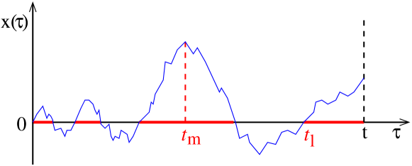
In this paper, we consider three global quantitites for a time series of duration starting at the origin. They are respectively (i) the occupation time , i.e., the cumulative time where with denoting the Heaviside step function: for and for (ii) the time of the maximum in , and (iii) the time of the last passage, before , of the process to (see Fig. 1). All three observables are random variables each supported over . For example, for a time series representing the value of a stock over a maturity period , normalized to the value when bought, the occupation time is the time where it exhibits profit, the time of the maximum is the best time to sell, and the last-passage time indicates the last time the value changes from profit to loss or vice-versa. For a Brownian time series, the marginal distributions of these random varibles were computed by Lévy levy1940 and quite remarkably, they all follow the same arcsine law for or , where the name originates from the corresponding arcsine cumulative distribution, i.e., .
These three quantities are relevant in various complex systems and have been studied a for a wide variety of stochastic processes with diverse applications. The occupation time has been analyzed, e.g., for random jump processes andersen1954 , renewal and resetting processes lamperti1958 ; godreche2001 ; burov2011 ; den_hollander2019 , Gaussian Markov processes dhar1999 ; de_smedt2001 and has played an important role in the context of persistence in nonequilibrium systems bray2013 ; newman1998 ; drouffe1998 ; toroczkai1999 ; baldassarri1999 . Furthermore, it has been studied for various other processes such as opinions in voter models cox1983 , blinking nanacrystals margolin2005 , diffusion in a disordered environment majumdar2002 ; sabhapandit2006 ; radice2020 ; kay2023 , a class of spin glass models majumdar2002b , sub- and superdiffusive processes bel2005 ; barkai2006 ; delvecchio2024 ; sadhu2018 , random acceleration process boutcheng2016 , active run-and-tumble process singh2019 ; bressloff2020 ; mukherjee2023 , permutation genrated random walks fang2021 and for a noninteracting Brownian gas burenev2024 . Experimentally, the occupation time has been studied for colloidal quantum dots brokmann2003 ; stefani2009 , thermodynamic currents barato2018 , and coherently driven optical resonators ramesh2024 .
The time at which the global maximum occurs in a process of total duration has been studied extensively in the context of extreme-value statistics majumdar2010 ; majumdar2020 ; majumdar2024 . Examples include Brownian motion with drift shepp1979 ; buffet2003 ; MB2008 , permutation-generated random walks fang2021 , Brownian and anomalous diffusion with constraints MRKY08 ; randon-furling2007 ; schehr2010 ; majumdar2010hitting ; MMS21 , random acceleration process majumdar2010acceleration , heterogeneous diffusion singh2022 ; delvecchio2024 , run-and-tumble process singh2019 ; MMS21 , fractional Brownian motion delorme2016 ; sadhu2018 , processes with stochastic resetting MMS21 ; singh2021 . The lack of symmetry of the distribution of around its mean in a stationary time series has been shown to be a sufficient condition that the underlying dynamics violates detailed balance MMS21 ; MMS22 . Another application of of a -d process is to estimate the mean perimeter and the mean area of the convex hull of a -d process randon-furling2009 ; majumdar2010convex ; reymbaut2011 ; dumonteil2013 ; rtp_ch2020 ; MMSS21 ; singh2022convex . Other applications appear in finance dale1980 ; MB2008 ; chicheportiche2014 and sports clauset2015 .
The last-passage time has been studied also for diffusion in extermal potentials bao2006 ; comtet2020 , in imhomogeneous environement delvecchio2024 , and in permutation-generated random walks fang2021 . For applications, it was considered for electronic ring oscillators leung2004 ; robson2014 and for investigating fission bao2004 . It has been used for setting up Monte Carlo methods to calculate capacitances on systems with flat or spherical surfaces hwang2006 ; yu2021 . The last-passage time has also been applied to devise optimal inspection policies of degrading systems barker2009 and in finance nikeghbali2013 .
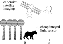
Although the marginal distributions of these three global quantities , and have been studied for various stochastic time series as mentioned above, their mutual correlations, encoded in pairwise joint distributions, have not been studied to the best of our knowledge. As an example why these joint distributions are of interest, one could consider animal movement as a toy application. The development of low-orbiting micro satellites like the KITSUNE 6U satellite azami2022 makes the observation with high-temporal imaging possible such that in the future even animals can be observed, but at high cost. For example, tigers live in a mixed habitats consisting of deep woods and open grass land mazak1981 , see Fig. 2. Here, it makes only sense to buy expensive high-resolution satellite footings, for times the animal is in the open land. We assume that one has to decide which of the expensive images to buy before being able to look at them. Clearly, the best time footage to buy is the time where the animal is maximally displaced from the wooded region so that it is completely visible. However, is not known apriori and has a broad distribution distributed all over (as in the arcsine law for a one dimensional Brownain motion). So, it is not clear which time or times to choose. However, suppose we have some knowledge about the occupation time that corresponds to the cumulative time an animal spends in the open land. This could be measured easily with a low-cost and low-weight sensor which does not annoy the animal considerably, i.e., without relatively heavy GPS or time-stamping facilities. Conditioned on the knowledge of , a representative value of with high probability may emerge and one can then buy the footage corresponding to that. We will show an explicit example of that for the -d Brownian motion later (in the right panel of Fig. 4). Thus, exploiting the correlations between two global quantities in a model, here for a simple random walk, allows for a much better targeted analysis of the data. This is certainly true for other systems like atoms, molecules, or microbes, or other time series data like wind speeds, stock markets or public opinions, which are in many cases only partially observable.
To gain better insights into the correlations between these three global quantities, one needs to compute the pairwise joint distributions of them analytically in a simple model time series. In this Letter, we consider the simplest and most ubiquitous time series, namely a one dimensional Brownian motion of duration . For this model, the marginal distributions of all three quantities are identically given by the arcsine law, as mentioned earlier. Here we compute exactly the pairwise joint distributions and demonstrate that, even in this simple model, they exhibit a rather rich, nontrivial, and unexpected behavior, not at all compatible with, say, standard linear correlations.
Model and quantities of interest. More precisely, we consider a one dimension Brownian motion of duration evolving via the Langevin equation , where is the diffusion constant and is a Gaussian white noise with zero mean and delta correlator: . We assume that the process starts at the origin, i.e., . We consider the three classical observables, , and defined before and depicted schematically in Fig. (1). Each of them has the same marginal PDF (probability distribution function) given by levy1940
| (1) |
valid for all , where , or . The scaling function (for ) is independent of the index and the diffusion constant . While the marginal PDF’s of these fractions are identical, it is clear that they are correlated with each other. Our goal is to compute the bivariate joint distributions
| (2) | |||||
The subscripts , and refer respectively to , and . We will show that these three joint distributions are highly nontrivial and are rather different from each other. We compute them exactly using the so called -path decomposition method first proposed in Refs. MC2004 ; MC2005 and then used subsequently in numerous other related problems majumdar2005 ; MRKY08 ; PCMS13 ; MMS2019 ; MMS2020 ; MMS21 ; MMSS21 ; MMS22 . Below we outline the main ideas leading to the results and the details of the derivations are presented in the Supplemental Material (SM) SM .
Last-passage time and occupation time . First, we focus on computing the , because this is the simplest of the three. The idea is to first express the joint distribution as where denotes the conditional distribution of given and , while is the marginal distribution of given in Eq. (1). We split the total duration into two intervals: () and () . Consequently, can also be split into two parts , where the two random variables and are independent of each other, for a given fixed . The idea then is to compute the PDF of each of them separately and then convolute them to compute the full conditional probability.
For the first interval, the Brownian motion starts at the origin at and ends at the origin at . For such a Brownian bridge, it is well known that the PDF of the occupation time is flat feller1957 , i.e., .
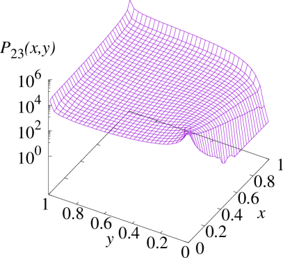
Concerning the second interval, the process crosses zero for the last time at , it may either cross from above or from below, each with equal probability . For the first case, the process stays below zero, so , in the other case we have . Thus, we obtain . The distribution for the total occupation time is given by the convolution . By applying the arcsine result for the marginal distribution of from Eq. (1), one obtains for , expressed in the scaling form, ,
| (3) | |||||
which is shown in Fig. 3. To obtain a better impression of the distribution, a cross section at is also displayed on the right panel of Fig. 3.
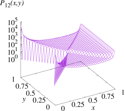
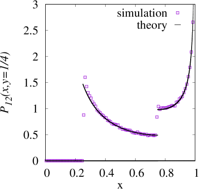
Here, also a comparison with numerical simulations of random walks is included. For that purpose, standard random walks, starting at zero, are performed with a certain number of steps. Thus, the position at step is given by , where are identically and independently distribution standard Gaussian numbers, numerically drawn by using the Box-Muller approach parctical_guide2015 . The data can be scaled to any time span simply by rescaling the times to . This approximates Brownian motion with step size . Here, we use and average over independent walks. Note that only the signs of the positions are important here, so no position rescaling is necessary. All three times , and can be directly read off from the time series and used to create corresponding joint histograms. The accuracy is limited by the discretised sampling at resolution , but this is sufficient for the present study, as visible in Fig. 3. For even better accuracy of and , one could use adaptive interval splitting approaches walter2022 .
Clearly, the joint distribution in (3) does not factorize demonstrating nontrivial correlations between the scaled variables and , which we computed explicitly. Interestingly, while the first-order correlation vanishes , higher order correlations are nonzero. For example, we find that and are weakly anticorrelated SM , also confirmed numerically.
Occupation time and time of maximum . To obtain the joint distribution , we again split the paths into two parts, here before and after , with the occupation time being the sum occupation times of the two parts and the distribution being the convolution of the possible values of for the parts. For both parts, including also the position of the maximum, one uses the Laplace transform separately and calculates the appearing propagators using Feynman-Kac formalism. This gives access to the exact triple Laplace transform with respect to , and , for details see the SM SM .
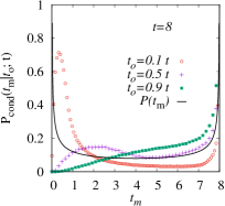
From this triple Laplace transform, we confirm that the two marginal distributions result in the arcsine law, and also obtain various covariance functions explicitly. For example, we get , , , and , which are all compatible with our numerical results.
Furthermore, in Fig. 4, the scaled joint PDF obtained from the numerical simulations is shown. Here, no discontinuities are present, but for fixed value of the scaled occupation time, the behavior of the probability changes considerably. For small scaled occupation times , the distribution is large for small times of the time of maximum, while for large occupation times it is opposite. This is also visible in the distribution of conditioned to a value of , as shown in the right panel of Fig. 4.
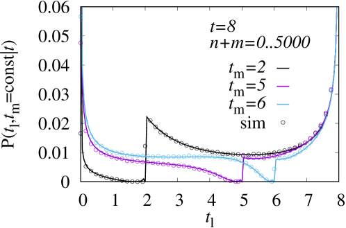
Last-passage time and time of maximum . Here the distribution is calculated again by the -path-decomposition approach SM . The interval is subdivided by the times and , where we treat the two cases and separately. In each of these cases, the three intervals are considered separately, and final results are obtained by convolution, for details see the SM SM . The final result reads
| (4) | |||||
with and . We have numerically evaluated the double sum in Eq. (4) using the mpfr library mpfr-lib , for an arbitrary choice of , by summing all terms with . In Fig. (5), we plot the resulting as a function of for three different fixed values of , and the simulation results for comparison. They match very well. The PDF exhibits a discontinuity at . While it vanishes very fast as from below, it approaches a nonzero constant when from above. In the SM, we also analyze the behavior of this discontinuity as a function of .
Conclusion. We have computed analytically, and verified numerically, the pairwise joint distributions for three global quantities (occupation time), (time of the maximum) and (last-passage time) for a one dimensional Brownian time series of duration . The main conclusion is that while the marginal distributions of these three variables all follow the same arcsine law, their joint distributions display very nontrivial and rich behaviors. Since Brownian motion is the simplest, and yet the most ubiquitous stochastic process appearing in many areas from physics to biology, our results may serve as a benchmark in many applications. Since joint distributions carry much more information about a system than the marginal distributions, obtaining them for other processes will be of high interest. In particular this will also allow for practical applications to investigate hidden properties by exploiting the knowledge of correlations, e.g., between two quantities where one is easily accessible, while the other is not.
Acknowledgements.
SNM acknowledges the Alexander von Humboldt foundation for the Gay Lussac-Humboldt prize that allowed a visit to the Physics department at Oldenburg University, Germany where most of this work was performed. The simulations were performed at the the HPC cluster ROSA, located at the University of Oldenburg (Germany) and funded by the DFG through its Major Research Instrumentation Program (INST 184/225-1 FUGG) and the Ministry of Science and Culture (MWK) of the Lower Saxony State.References
- (1) P. Fornasini, The Uncertainty in Physical Measurements — An Introduction to Data Analysis in the Physics Laboratory (Springer, New York, 2008).
- (2) V. L. Smith, Amer. Economic Rev. 66, 274 (1976), ISSN 00028282.
- (3) D. Houle, C. Pélabon, G. Wagner, and T. Hansen, Quarterly Rev.of Biol. 86, 3 (2011).
- (4) P. D. Delmas, Osteoporosis Intern. 9, S33 (1999), ISSN 1433-2965.
- (5) L. Bennani, F. Allali, S. Rostom, I. Hmamouchi, H. Khazzani, L. El Mansouri, L. Ichchou, F. Z. Abourazzak, R. Abouqal, and N. Hajjaj-Hassouni, Clinical Rheumatology 28, 1283 (2009), ISSN 1434-9949.
- (6) T. A. Hillier, L. Lui, D. M. Kado, E. LeBlanc, K. K. Vesco, D. C. Bauer, J. A. Cauley, K. E. Ensrud, D. M. Black, M. C. Hochberg, et al., J. Bone Mineral Res. 27, 153 (2012), ISSN 0884-0431.
- (7) W. Pluskiewicz, P. Adamczyk, A. Werner, M. Bach, and B. Drozdzowska, Biomedicines 11 (2023), ISSN 2227-9059.
- (8) D. M. Ragan, Structural Geology (Cambridge University Press, Cambridge, 2012).
- (9) S. D. Sloan, G. P. Tsoflias, D. W. Steeples, and P. D. Vincent, J. Appl. Geophys. 62, 281 (2007), ISSN 0926-9851.
- (10) H. Yuan, A. Z. Abdu, and L. Nielsen, Geophys. 88, MR141 (2023), ISSN 0016-8033.
- (11) J. A. Hildebrand, S. M. Wiggins, J. L. Driver, and M. R. Waters, Archaeological Prospection 14, 245 (2007).
- (12) R. Serfozo, Basics of Applied Stochastic Processes (Springer, Berlin, Heidelberg, 2009).
- (13) W. Feller, Introduction to Probability Theory and Its Applications, John Wiley & Sons, New York (1957).
- (14) P. Mörters, Y. Peres, Brownian motion, Vol. 30, Cam- bridge University Press, (2010).
- (15) R. M. Mazo, Brownian Motion: Fluctuations, Dynamics, and Applications (Oxford University Press, Oxford, 2008).
- (16) P. Doyle and J. Snell, Random walks and electric networks (Math. Ass. Amer., Washington DC, 1984).
- (17) J. Baz and G. Chacko, Financial derivatives: pricing, applications, and mathematics (Cambridge University Press, 2004)
- (18) A. Hirsa and S. N. Neftci, An introduction to the mathematics of financial derivatives (Academic Press, Amsterdam, 2014).
- (19) F. Schweitzer, Browning Agents and Active Particles : Collective Dynamics in the Natural and Social Sciences (Springer, Berlin, Heidelberg, 2007).
- (20) S. Redner, A guide to first-passage processes, Cambridge University Press, Cambridge, 2001.
- (21) S. N. Majumdar, Curr. Sci. 89, 2075 (2005).
- (22) S. N. Majumdar, Physica A 389, 4299 (2010).
- (23) A. J. Bray, S. N. Majumdar, and G. Schehr, Adv. in Phys. 62, 225 (2013).
- (24) L. A. Shepp, J. Appl. Proba. 16, 423 (1979).
- (25) E. Buffet, J. Appl. Math. Stoch. Anal. 16, 201 (2003).
- (26) J. Randon-Furling and S. N. Majumdar, J. Stat. Mech. P10008 (2007).
- (27) S. N. Majumdar, J. Randon-Furling, M. J. Kearney, M. Yor, J. Phys. A: Math. Theor. 41, 365005 (2008)
- (28) S. N. Majumdar, J.-P. Bouchaud, Quant. Fin. 8, 753 (2008).
- (29) S.N. Majumdar, A. Comtet, J. Randon-Furling, J. Stat. Phys. 138, 955 (2010).
- (30) G. Schehr and P. Le Doussal, J. Stat. Mech. P01009 (2010).
- (31) J. Rambeau and G. Schehr, Phys. Rev. E 83, 061146 (2011).
- (32) F. Mori, S. N. Majumdar, G. Schehr, Phys. Rev. Lett., 123, 200201 (2019).
- (33) F. Mori, S. N. Majumdar, and G. Schehr, Phys. Rev. E, 101, 052111 (2020).
- (34) P. Lévy, Compositio Mathematica 7, 283 (1940).
- (35) E. Sparre Andersen, Math. Scand. 1, 263 (1954).
- (36) J. Lamperti, Trans. Amer. Math. Soc. 88, 380 (1958).
- (37) C. Godrèche and J. M. Luck, J. Stat. Phys. 104, 489 (2001), ISSN 1572-9613.
- (38) S. Burov, E. Barkai, Phys. Rev. Lett. 107, 170601 (2011).
- (39) F. den Hollander, S. N. Majumdar, J. M. Meylahn, and H. Touchette, J. Phys. A: Math. Theor. 52, 175001 (2019).
- (40) A. Dhar and S. N. Majumdar, Phys. Rev. E 59, 6413 (1999).
- (41) G. De Smedt, C. Godrèche, and J. M. Luck, J. Phys. A: Math. Gen. 34, 1247 (2001).
- (42) T. J. Newman and Z. Toroczkai, Phys. Rev. E 58, R2685 (1998).
- (43) J.-M. Drouffe and C. Godrèche, J. Phys. A 31, 9801 (1998).
- (44) Z. Toroczkai, T. J. Newman, and S. Das Sarma, Phys. Rev. E 60, R1115 (1999).
- (45) A. Baldassarri, J.-P. Bouchaud, I. Dornic, and C. Godrèche, Phys.Rev. E 59, R20 (1999).
- (46) J. T. Cox and D. Griffeath, Annals Prob. 11, 876 (1983), ISSN 00911798.
- (47) G. Margolin and E. Barkai, Phys. Rev. Lett. 94, 080601 (2005).
- (48) S. N. Majumdar and A. Comtet, Phys. Rev. Lett. 89, 060601 (2002).
- (49) S. Sabhapandit, S. N. Majumdar, and A. Comtet, Phys. Rev. E 73, 051102 (2006).
- (50) M. Radice, M. Onofri, R. Artuso, and G. Pozzoli, Phys. Rev. E 101, 042103 (2020).
- (51) T. Kay and L. Giuggioli, J. Phys. A: Math. Theor. 56, 345002 (2023).
- (52) S. N. Majumdar and D. S. Dean, Phys. Rev. E 66, 041102 (2002).
- (53) G. Bel and E. Barkai, Phys. Rev. Lett. 94, 240602 (2005).
- (54) E. Barkai, J. Stat. Phys. 123, 883 (2006).
- (55) G, Del Vecchio Del Vecchio and S. N. Majumdar, arXiv preprint: arXiv:2410.22097
- (56) T. Sadhu, M. Delorme, K. J. Wiese, Phys. Rev. Lett. 120, 040603 (2018).
- (57) H. J. O. Boutcheng, T. B. Bouetou, T. W. Burkhardt, A. Rosso, A. Zoia, K. T. Crepin, J. Stat. Mech. 053213 (2016).
- (58) P. Singh and A. Kundu, J. Stat. Mech. 083205 (2019).
- (59) P. C. Bressloff, Phys. Rev. E 102, 042135 (2020).
- (60) S. Mukherjee and N. R. Smith, Phys. Rev. E 107, 064133 (2023).
- (61) X. Fang, H. L. Gan, S. Holmes, H. Huang, E. Peköz, A. Röllin, and W. Tang, J. Appl. Prob. 58, 851–867 (2021).
- (62) I. N. Burenev, S. N. Majumdar, A. Rosso, Phys. Rev. E, 109, 044150 (2024).
- (63) X. Brokmann, J.-P. Hermier, G. Messin, P. Desbiolles, J.-P. Bouchaud, and M. Dahan, Phys. Rev. Lett. 90, 120601 (2003).
- (64) F. D. Stefani, J. P. Hoogenboom, and E. Barkai, Physics Today 62 (2), 34 (2009).
- (65) A. C. Barato, E. Roldán, I. A. Martínez, and S. Pigolotti, Phys. Rev. Lett. 121, 090601 (2018).
- (66) V. G. Ramesh, K. J. H. Peters, and S. R. K. Rodriguez, Phys. Rev. Lett. 132, 133801 (2024).
- (67) S. N. Majumdar, A. Pal, and G. Schehr, Phys. Rep. 840, 1 (2020).
- (68) S. N. Majumdar and G. Schehr, Statistics of Extremes and Records in Random Sequences, Oxford University Press, (2024).
- (69) S. N. Majumdar, A. Rosso, and A. Zoia, Phys. Rev. Lett. 104, 020602 (2010).
- (70) F. Mori, S. N. Majumdar, and G. Schehr, Europhys. Lett. 135, 30003 (2021).
- (71) S. N. Majumdar, A. Rosso, and A. Zoia, J. Phys. A: Math. Theor. 43, 115001 (2010).
- (72) P. Singh, Phys. Rev. E 105, 024113 (2022).
- (73) M. Delorme, K. J. Wiese, Phys. Rev. E 94, 052105 (2016).
- (74) P. Singh and A. Pal, Phys. Rev. E 103, 052119 (2021).
- (75) F. Mori, S. N. Majumdar, and G. Schehr, Phys. Rev. E 106, 054110 (2022).
- (76) J. Randon-Furling, S. N. Majumdar, and A. Comtet, Phys. Rev. Lett. 103, 140602 (2009).
- (77) S. N. Majumdar, A. Comtet, and J. Randon-Furling, J. Stat. Phys. 138, 955 (2010).
- (78) A. Reymbaut, S. N. Majumdar, and A. Rosso, J. Phys. A: Math. Theor. 44, 415001 (2011).
- (79) E. Dumonteil, S. N. Majumdar, A. Rosso, and A. Zoia, Proc. Natl. Aca. Sci. U. S. A., 110, 4239 (2013).
- (80) A. K. Hartmann, S. N. Majumdar, H. Schawe, and G. Schehr, J. Stat. Mech. 053401 (2020).
- (81) S. N. Majumdar, F. Mori, H. Schawe, and G. Schehr, Phys. Rev. E 103, 022135 (2021).
- (82) P. Singh, A. Kundu, S. N. Majumdar, and H. Schawe, J. Phys. A.: Math. Theor. 55, 225001 (2022).
- (83) C. Dale and R. Workman, Financ. Analysts J. 36, 71 (1980).
- (84) R. Chicheportiche and J.-P. Bouchaud, in: R. Metzler, G. Oshanin, and S. Redner (eds.), First-Passage Phenomena and Their Applications, 447 (World Scientific, Singapore 2014).
- (85) A. Clauset, M. Kogan, and S. Redner, Phys. Rev. E 91, 062815 (2015).
- (86) J. D. Bao and Y. Jia, J. Stat. Phys. 123, 861 (2006).
- (87) A. Comtet, F. Cornu, and G. Schehr, J. Stat. Phys. 181, 1565 (2020).
- (88) B. H. Leung, IEEE Trans. Circuits Syst. I: Regular Papers, 51, 471 (2004).
- (89) S. Robson, B. Leung, and G. Gong, IEEE Trans. Circuits Syst. II: Express Briefs 61(12), 937 (2014).
- (90) J. D. Bao, and Y. Jia, Phys. Rev. C 69, 027602 (2004).
- (91) C.-O. Hwang and J. A. Given, Phys. Rev. E 74, 027701 (2006).
- (92) U. Yu, Y.-M. Lee, and C.-O. Hwang, J. Sci. Comput. 88, 82 (2021).
- (93) C. T. Barkar and M. J. Newby, Reliability Engineering & System Safety, 94, 33 (2009).
- (94) A. Nikeghbali and E. Platen, Finance Stoch. 17, 615 (2013).
- (95) M. H. Bin Azami, N. C. Orger, V. H. Schulz, T. Oshiro, and M. Cho, Remote Sensing 14 (2022).
- (96) V. Mazák, Mammalian Species pp. 1–8 (1981), ISSN 0076-3519.
- (97) S.N. Majumdar and A. Comtet, Phys. Rev. Lett., 92, 225501 (2004).
- (98) S.N. Majumdar and A. Comtet, J. Stat. Phys. 119, 777 (2005).
- (99) A. Perret, A. Comtet, S. N. Majumdar, G. Schehr, Phys. Rev. Lett., 111, 240601 (2013).
- (100) See Supplemental Material.
- (101) A. K. Hartmann, Big Practical Guide to Computer Simulations (World Scientific, Singapore 2015).
- (102) B. Walter and K. J. Wiese, Phys. Rev. E 101, 043312 (2020).
-
(103)
MPFR multi precision floating point
library,
https://www.mpfr.org/