A harmonic oscillator in nonadditive statistics and a novel transverse momentum spectrum in high-energy collisions

Abstract

It is widely observed that particles produced in high-energy collisions follow a power-law distribution. One such power-law distribution used extensively in the phenomenological studies owes its origin to nonadditive statistics proposed by C. Tsallis. In this article, we derive a novel nonadditive generalization of the conventional Bose-Einstein distribution using a single-mode harmonic oscillator. The approach taken in this paper eliminates the need of a regularization procedure proposed in previous works. We observe that the spectra of the bosonic particles like the pions and kaons produced in high-energy collisions are well-described by the nonadditive bosonic distribution derived in this paper.

I Introduction

Transverse momentum spectra of the hadrons produced in high-energy collisions are important experimental observables that provide information on dynamics of the system and the freeze-out parameters like temperature. Hence, it is important to understand them from a theoretical perspective and these efforts constitute an active field of research. Because of a large number of particles produced in these collisions, methods of statistical mechanics in describing particle spectra can be applied. However, the conventional Boltzmann-Gibbs statistics, that yields exponential distributions, is unable to describe experimental data at larger momentum. For example, for the $\pi^{+}$ spectra in a p-p collision at $\sqrt{s}=900$ GeV measured by the ALICE collaboration alicepi , the experimental spectra obtained in high-energy collisions start deviating from being exponential at a transverse momentum around 0.5 GeV. On the other hand, power-law distributions successfully describe the transverse momentum distributions of such particles TsCMS ; TsALICE ; abcp ; maciejepjc up to a large momentum. These references utilize a certain class of power-law distributions that owes its origin to nonadditive statistics proposed by C. Tsallis Tsal88 .

Nonadditive statistics is a generalization of the Boltzmann-Gibbs statistics for systems having fluctuations and long-range correlation. Such a generalization often features the following quasi-exponential function:

$$\exp_{q}\left(-\frac{\varepsilon_{p}}{T}\right)=\left(1+\frac{q-1}{T}\varepsilon_{p}\right)^{-\frac{1}{q-1}},$$ (1)

where $q$ is the entropic parameter, $\varepsilon_{p}=\sqrt{p^{2}+m^{2}}$ is the single particle energy of a particle of the mass $m$ and 3-momentum $\vec{p}$ ($|\vec{p}|\equiv p$), and $T(\equiv\beta^{-1})$ is temperature. When $q$ approaches 1, Eq. (1) approaches toward the conventional exponential function.

The $q$ parameter is shown to be connected to the relative variance in thermodynamic quantities (e.g. temperature) Wilk00 ; Wilk09 . The $q$ parameter can also be computed in terms of the parameters in quantum chromodynamics like $N_{c}$ (no. of colours) and $N_{f}$ (no. of flavours) deppmanprdq by studying the scaling properties of the Yang-Mills theory. The entropic parameter has been utilized to estimate the relaxation and correlation times of a hadronizing system maciejprd or to propose a generalized Boltzmann transport equation whose stationary state solution is given by the $q$-exponential function lavagnopla ; wilkosada ; Biro:2012ix . There are many instances where natural systems exhibit behaviour that is better described by generalized statistical mechanics, of which nonadditive statistics is a prominent example.

It is important to establish a connection between the single-particle distribution used in the literature and the fundamental approaches of physics like statistical mechanics considered in the present work. It has been shown that the phenomenological nonadditive distributions can be derived TBParvan1 ; TBParvan2 by extremizing nonadditive entropy proposed by Tsallis Tsal88 . However, while deriving classical and quantum distributions, divergence was encountered and a regularization scheme had to be proposed. In this article, we take a different approach in which we derive a novel bosonic nonadditive single-particle distribution considering a single-mode harmonic oscillator. This approach eliminates the need of a regularization scheme. We use this nonadditive bosonic distribution to model particle transverse momentum distribution and compare our results with experimentally observed spectra. Highlights of the present work are as follows:

• As far as our knowledge goes, the nonadditive transverse momentum spectrum in Eq. (III) has been derived for the first time in the literature considering a single-mode harmonic oscillator.

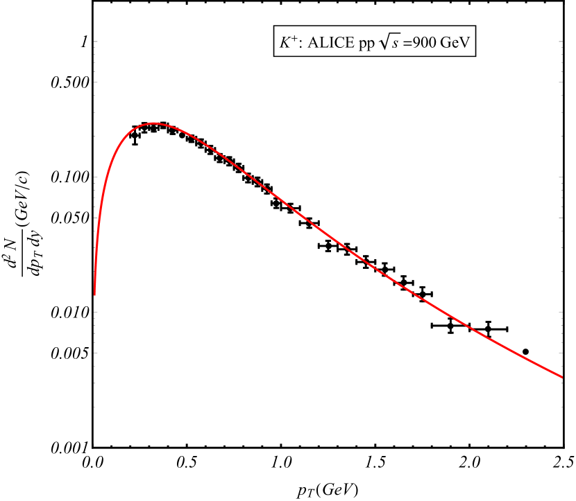
Figure 4: Description of $K^{+}$ spectrum provided in Ref. alicepi using Eq. (15): The parameter values are: $q=0.853\pm 0.01213$, $T=0.0657\pm 0.01433$ GeV, $R=3.994\pm 1.083$ fm, $\chi^{2}$/NDF = 5.357/24.

• While the conventional Bose-Einstein distribution describes only very low momentum data, the nonadditive transverse momentum spectrum derived in Eq. (III) describes experimental data well for the whole range of transverse momenta considered in our analyses (Figs. 4 and 4).

• Our approach eliminates the need of regularization of transverse momentum spectra.

The rest of the article will be devoted to describing the mathematical model, exploring different limits of our result and comparing it with experimental data.

II Mathematical model from nonadditive statistical mechanics

II.1 Equilibrium set of probabilities

Nonadditive statistical mechanics is based on the following definition of entropy Tsal88 ,

$$S={{\sum}}\limits_{i}\frac{p_{i}^{q}-p_{i}}{1-q},$$ (2)

where $q$ is a real parameter, and the probabilities of micro-states $\{p_{i}\}$ follow the normalization condition,

$$\varphi=\sum\limits_{i}p_{i}-1=0.$$ (3)

The definition of average expectation values in the normalized (or the first) scheme is given by Tsal98 ,

$$\langle Q\rangle=\sum\limits_{i}p_{i}Q_{i}.$$ (4)

The thermodynamic potential $\Omega$ of the grand canonical ensemble can be written as,

$$\Omega = \langle H\rangle-TS-\mu\langle N\rangle$$ (5)

$$= \sum\limits_{i}p_{i}\left[E_{i}-\mu N_{i}-T\frac{p_{i}^{q-1}-1}{1-q}\right],$$

where $\langle H\rangle=\sum_{i}p_{i}E_{i}$ is the mean energy of the system, $\langle N\rangle=\sum_{i}p_{i}N_{i}$ is the mean number of particles, and $E_{i}$ and $N_{i}$ are the energy and number of particles, respectively, in the $i$-th microscopic state of the system. The set of equilibrium probabilities $\{p_{i}\}$ can be found from local extremization of the thermodynamic potential $\Omega$ (subjected to probability normalization constraint) by the method of the Lagrange multipliers (see, for example, Ref. Jaynes2 ). In terms of a modified potential $\Phi$, defined below, the equilibrium set of probabilities can be found from the second of the following equations:

$$\Phi = \Omega-\lambda\varphi,$$ (6)

$$\frac{\partial\Phi}{\partial p_{i}} = 0,$$ (7)

where $\lambda$ is an arbitrary real constant.

Substituting Eqs. (3) and (4) into Eqs. (6) and (7), we obtain the equilibrium probabilities of the grand canonical ensemble (for the normalized statistics) as TBParvan2

$$p_{i}=\left[1+\frac{q-1}{q}\frac{\Lambda-E_{i}+\mu N_{i}}{T}\right]^{\frac{1}{q-1}},$$ (8)

subjected to probability normalization,

$${\sum}\limits_{i}\left[1+\frac{q-1}{q}\frac{\Lambda-E_{i}+\mu N_{i}}{T}\right]^{\frac{1}{q-1}}=1,$$ (9)

where $\Lambda\equiv\lambda-T$ and $\partial E_{i}/\partial p_{i}=\partial N_{i}/\partial p_{i}=0$. $\Lambda$ is related to the partition function that also helps define an effective temperature. In the Gibbs limit $q\to 1$, the probability $p_{i}=\exp[(\Lambda-E_{i}+\mu N_{i})/T]$, where $\Lambda=-T\ln Z$ is the thermodynamic potential of the grand canonical ensemble and $Z=\sum_{i}\exp[-(E_{i}-\mu N_{i})/T]$ is the partition function.

II.2 Nonadditive average represented in terms of Boltzmann-Gibbs average

Using the integral representation of the gamma functions Abramowitz for $q<1$, probability normalization and average values can be rewritten as TBParvan2 ,

$$p_{i} = \frac{1}{\Gamma\left(\frac{1}{1-q}\right)}\int\limits_{0}^{\infty}t^{\frac{q}{1-q}}e^{-t\left[1+\frac{q-1}{q}\frac{\Lambda-E_{i}+\mu N_{i}}{T}\right]}dt;$$

$$\sum_{i}p_{i} = \frac{1}{\Gamma\left(\frac{1}{1-q}\right)}\int\limits_{0}^{\infty}t^{\frac{q}{1-q}}e^{-t\left[1+\frac{q-1}{q}\frac{\Lambda-\Omega_{\text{G}}\left(\beta^{\prime}\right)}{T}\right]}dt=1.$$ (10a)

$$\langle Q\rangle = \frac{1}{\Gamma\left(\frac{1}{1-q}\right)}\int\limits_{0}^{\infty}t^{\frac{q}{1-q}}e^{-t\left[1+\frac{q-1}{q}\frac{\Lambda}{T}\right]}Z_{\text{G}}\left(\beta^{\prime}\right)\langle Q\rangle_{\text{G}}(\beta^{\prime})dt,$$ (10b)

where

$$\Omega_{\text{G}}\left(\beta^{\prime}\right) = -\frac{1}{\beta^{\prime}}\ln Z_{\text{G}}\left(\beta^{\prime}\right);~{}~{}Z_{\text{G}}\left(\beta^{\prime}\right)=\sum\limits_{i}e^{-\beta^{\prime}(E_{i}-\mu N_{i})};$$

$$\langle Q\rangle_{\text{G}}\left(\beta^{\prime}\right) = \frac{1}{Z_{\text{G}}\left(\beta^{\prime}\right)}\sum\limits_{i}Q_{i}e^{-\beta^{\prime}(E_{i}-\mu N_{i})};$$

$$\text{and}~{}~{}~{}~{}\beta^{\prime} = t(1-q)/qT.$$ (11)

The main results of this section are Eqs. (10) and (10b) that will be used to calculate nonadditive single particle distributions ($\langle n_{p\sigma}\rangle$) in terms of Boltzmann-Gibbs single particle distributions ($\langle n_{p\sigma}\rangle_{\text{G}}$). $n_{p\sigma}$ is the number of particles (of the mass $m$ and energy $\varepsilon_{p}$) in a micro-state $i$ with three-momentum $p=\sqrt{\varepsilon_{p}^{2}-m^{2}}$, such that $E_{i}=\sum n_{p\sigma}\varepsilon_{p}$ and $N_{i}=\sum n_{p\sigma}$ ($\sigma$ represents any quantum number like spin, for example).

II.3 Calculating nonadditive single-particle distributions

Using Eq. (10b), we can express the nonadditive single-particle distributions in terms of the Boltzmann-Gibbs single-particle distributions through the following integral,

$$\langle n_{p\sigma}\rangle = \frac{1}{\Gamma\left(\frac{1}{1-q}\right)}\int\limits_{0}^{\infty}t^{\frac{q}{1-q}}e^{-t\left[1+\frac{q-1}{q}\frac{\Lambda}{T}\right]}~{}Z_{\text{G}}\left(\beta^{\prime}\right)~{}\langle n_{p\sigma}\rangle_{\text{G}}(\beta^{\prime})~{}dt.$$ (12)

In the above integral, $\Lambda$ is calculated from probability normalization given by Eq. (10) for a given set of $q$ and $T$. We are able to find a closed analytical form of Eq. (12) for a single-mode harmonic oscillator as shown below.

In the Boltzmann-Gibbs statistics, the (normal ordered) partition function for a single-mode harmonic oscillator (with frequency $\varepsilon_{p}$) is given by (chemical potential is set equal to zero),

$$Z_{\text{G}}(\beta)=\frac{1}{1-e^{-\beta\varepsilon_{p}}},$$ (13)

and it yields the Boltzmann-Gibbs Bose-Einstein single-particle distribution,

$$\langle n_{p\sigma}\rangle_{\text{G}}(\beta) = -\frac{1}{\beta}\frac{\partial\ln Z_{\text{G}}}{\partial\varepsilon_{p}}$$ (14)

$$= \frac{1}{e^{\beta\varepsilon_{p}}-1}.$$

In what follows, we generalize the Boltzmann-Gibbs Bose-Einstein distribution obtained in Eq. (14) for nonadditive statistics by putting Eqs. (13) and (14) in Eq. (12):

$$\langle n_{p\sigma}\rangle=\frac{1}{\Gamma\left(\frac{1}{1-q}\right)}\int\limits_{0}^{\infty}t^{\frac{q}{1-q}}e^{-t\left[1+\frac{q-1}{q}\frac{\Lambda}{T}\right]}~{}e^{-\beta^{\prime}\Omega_{\text{G}}(\beta^{\prime})}~{}\langle n_{p\sigma}\rangle_{\text{G}}(\beta^{\prime})~{}dt$$ (15)

$$= \frac{1}{\Gamma\left(\frac{1}{1-q}\right)}\int\limits_{0}^{\infty}t^{\frac{q}{1-q}}e^{-t\left[1+\frac{q-1}{q}\frac{\Lambda}{T}\right]}~{}\frac{1}{1-e^{-\beta^{\prime}\varepsilon_{p}}}~{}\frac{1}{e^{\beta^{\prime}\varepsilon_{p}}-1}~{}dt$$

$$= \frac{1}{\Gamma\left(\frac{1}{1-q}\right)}\int\limits_{0}^{\infty}t^{\frac{q}{1-q}}e^{-t\left[1+\frac{q-1}{q}\frac{\Lambda}{T}\right]}~{}\sum_{n=0}^{\infty}e^{-n\beta^{\prime}\varepsilon_{p}}~{}\left[\sum_{r=0}^{\infty}e^{-r\beta^{\prime}\varepsilon_{p}}-1\right]~{}dt$$

$$= \frac{1}{\Gamma\left(\frac{1}{1-q}\right)}\sum_{n=0}^{\infty}\sum_{r=0}^{\infty}\int\limits_{0}^{\infty}t^{\frac{q}{1-q}}e^{-t\left[1+\frac{q-1}{q}\frac{\Lambda}{T}\right]}~{}e^{-(n+r)\beta^{\prime}\varepsilon_{p}}~{}dt-\frac{1}{\Gamma\left(\frac{1}{1-q}\right)}\sum_{n=0}^{\infty}\int\limits_{0}^{\infty}t^{\frac{q}{1-q}}e^{-t\left[1+\frac{q-1}{q}\frac{\Lambda}{T}\right]}~{}e^{-n\beta^{\prime}\varepsilon_{p}}~{}dt$$

$$= {\sum}_{n=0}^{\infty}{\sum}_{r=0}^{\infty}\frac{1}{\left(1+\frac{1-q}{qT}\left[(n+r)\varepsilon_{p}-\Lambda\right]\right)^{\frac{1}{1-q}}}-{\sum}_{n=0}^{\infty}\frac{1}{\left(1+\frac{1-q}{qT}[n\varepsilon_{p}-\Lambda]\right)^{\frac{1}{1-q}}}$$

$$= \left(\frac{qT}{(1-q)\varepsilon_{p}}\right)^{\frac{1}{1-q}}\left[\zeta\left(\frac{q}{1-q},\frac{qT}{(1-q)\varepsilon_{p}}-\frac{\Lambda}{\varepsilon_{p}}\right)+\left(1-\frac{qT}{(1-q)\varepsilon_{p}}+\frac{\Lambda}{\varepsilon_{p}}\right)\zeta\left(\frac{1}{1-q},\frac{qT}{(1-q)\varepsilon_{p}}-\frac{\Lambda}{\varepsilon_{p}}\right)\right]$$

$$-\left(\frac{qT}{(1-q)\varepsilon_{p}}\right)^{\frac{1}{1-q}}\zeta\left(\frac{1}{1-q},\frac{qT}{(1-q)\varepsilon_{p}}-\frac{\Lambda}{\varepsilon_{p}}\right)$$

$$= \left(\frac{qT}{(1-q)\varepsilon_{p}}\right)^{\frac{1}{1-q}}\left[\zeta\left(\frac{q}{1-q},\frac{qT}{(1-q)\varepsilon_{p}}-\frac{\Lambda}{\varepsilon_{p}}\right)-\left(\frac{qT}{(1-q)\varepsilon_{p}}-\frac{\Lambda}{\varepsilon_{p}}\right)\zeta\left(\frac{1}{1-q},\frac{qT}{(1-q)\varepsilon_{p}}-\frac{\Lambda}{\varepsilon_{p}}\right)\right]$$

Using a similar procedure, the probability normalization, Eq. (10), can be written as:

$$\left(\frac{qT}{(1-q)\varepsilon_{p}}\right)^{\frac{1}{1-q}}\zeta\left(\frac{1}{1-q},\frac{qT}{(1-q)\varepsilon_{p}}-\frac{\Lambda}{\varepsilon_{p}}\right)=1.$$ (16)

Solving the above equation gives us the value of $\Lambda$. In the above equations $\zeta(s,a)$ is the Hurwitz zeta function defined as follows:

$$\zeta(s,a)=\sum_{n=0}^{\infty}\frac{1}{(a+n)^{s}},\forall n\ni a+n\neq 0,\Re(s)>1.$$ (17)

We also use the following identity,

$$\sum_{m,n=0}^{\infty}\frac{1}{(b+m+n)^{s}}=\zeta(s-1,b)+(1-b)\zeta(s,b),\forall b>0.$$ (18)

II.4 Single particle distribution: some observations

Eq. (15) is a generalization of the conventional bosonic single-particle distribution within the scope of the nonadditive statistics. When $q$ approaches 1, Eq. (15) approaches the conventional Boltzmann-Gibbs Bose-Einstein (BGBE) distribution, as seen in Fig. 2. The emergence of the BGBE distribution can also be understood by taking the $q\rightarrow 1$ limit of the fifth line of Eq. (15):

$${\sum}_{n=0}^{\infty}{\sum}_{r=0}^{\infty}\frac{1}{\left(1+\frac{1-q}{qT}\left[(n+r)\varepsilon_{p}-\Lambda\right]\right)^{\frac{1}{1-q}}}-{\sum}_{n=0}^{\infty}\frac{1}{\left(1+\frac{1-q}{qT}[n\varepsilon_{p}-\Lambda]\right)^{\frac{1}{1-q}}}\xrightarrow{q\rightarrow 1}\frac{\exp[\beta(\varepsilon_{p}+\Lambda)]}{(\exp(\beta\varepsilon_{p})-1)^{2}}=\frac{1}{\exp(\beta\varepsilon_{p})-1},$$

where we use Eq. (13) and the relationships below Eq. (9) to find that $\exp(\beta\Lambda)=Z_{\text{G}}^{-1}=1-\exp(-\beta\epsilon_{p})$.

We also observe in Fig. 2 that as the single-particle energy begins surpassing other energy scales, the nonadditive BE distribution in Eq. (15) starts approaching the classical nonadditive Maxwell-Boltzmann (MB) distribution given below:

$$\langle n_{p\sigma}\rangle\xrightarrow{\varepsilon_{p}\gg T,\Lambda}\left(1+\frac{1-q}{qT}\varepsilon_{p}\right)^{\frac{1}{q-1}}.$$ (20)

The distribution above is dual to the widely-used phenomenological nonadditive distribution:

$$\left(1+\frac{1-q}{qT}\varepsilon_{p}\right)^{\frac{1}{q-1}}\xrightarrow{q\rightarrow 1/q^{\prime}}\left(1+\frac{q^{\prime}-1}{T}\varepsilon_{p}\right)^{-\frac{q^{\prime}}{q^{\prime}-1}}.$$ (21)

The classical distribution can also be obtained by imposing the factorization approximation hasegawa on Eq. (15) in high energy limit. The factorization approximation (as well as assuming $\varepsilon_{p}\gg T,\Lambda$) amounts to making the following substitution (for a summation index $N\in\mathbb{Z}^{\geq}$):

$$\left(1+\frac{1-q}{qT}[N\varepsilon_{p}-\Lambda]\right)^{-\frac{1}{1-q}}\approx\left(1+\frac{1-q}{qT}\varepsilon_{p}\right)^{-\frac{N}{1-q}}.$$ (22)

Using Eq. (22) and performing the series summation in Eq. (15) lead us to:

$$\langle n_{p\sigma}\rangle_{\text{F}}\approx\left(1+\frac{1-q}{qT}\varepsilon_{p}\right)^{\frac{1}{q-1}},$$ (23)

where ‘F’ stands for a factorized single-particle distribution. In the lower energy region, $\langle n_{p\sigma}\rangle_{\text{F}}$ approaches being dual ($q\leftrightarrow 1/q^{\prime}$) to the phenomenological nonadditive Bose-Einstein distribution used in the literature tsq .

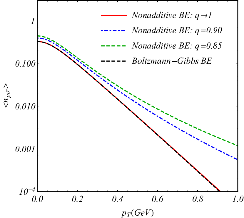
Figure 1: Variation of nonadditive BE distribution (Eq. (15)) for a particle having the mass of the pions (0.14 GeV) and temperature $T=0.1$ GeV for different entropic parameter $q$.

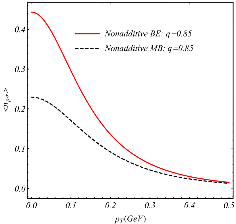
Figure 2: Nonadditive BE distribution in Eq. (15) ($m=0.14$ GeV, $T$ = 0.1 GeV) approaches classical nonadditive distribution when energy well surpasses temperature.

III Results and discussion

There have been many attempts to utilize the single-particle distributions to describe particle production in high-energy collisions. Experimentally observed transverse momentum distributions can be calculated from single-particle distributions $\langle n_{p\sigma}\rangle$ in the following way:

$$\frac{d^{2}N}{dp_{\text{T}}dy}=\frac{gV}{(2\pi)^{3}}\int\limits_{0}^{2\pi}d\phi~{}p_{\mathrm{T}}\varepsilon_{p}\langle n_{p\sigma}\rangle,$$ (24)

where $\phi$ is the azimuthal angle, $g$ is the degeneracy factor, $p_{\text{T}}$ is transverse momentum, and $V=4\pi R^{3}/3$ ($R$: radius) is the volume. Some of the approaches utilize the exponential Boltzmann-Gibbs (for low momena), or the phenomenological nonadditive power-law distributions. However, in this work, we utilize the single-particle distribution derived in Eq. (15) and obtain the following expression:

$$\frac{d^{2}N}{dp_{\text{T}}dy} = \frac{gV}{(2\pi)^{2}}p_{\mathrm{T}}m_{\mathrm{T}}\cosh(y)$$

$$\times\left(\frac{qT}{(1-q)\varepsilon_{p}}\right)^{\frac{1}{1-q}}\left[\zeta\left(\frac{q}{1-q},\frac{qT}{(1-q)\varepsilon_{p}}-\frac{\Lambda}{\varepsilon_{p}}\right)-\left(\frac{qT}{(1-q)\varepsilon_{p}}-\frac{\Lambda}{\varepsilon_{p}}\right)\zeta\left(\frac{1}{1-q},\frac{qT}{(1-q)\varepsilon_{p}}-\frac{\Lambda}{\varepsilon_{p}}\right)\right],$$

where single-particle energy (of a particle of the mass $m$ and momentum $\vec{p}\equiv\{\vec{p_{\text{T}}},p_{z}\}$) $\varepsilon_{p}=\sqrt{\vec{p}^{2}+m^{2}}$ is parameterized in terms of transverse mass $m_{\text{T}}=\sqrt{p_{\text{T}}^{2}+m^{2}}$ and rapidity $y$ such that $\varepsilon_{p}=m_{\text{T}}\cosh(y)$. Eq. (III) is the main result of our paper that we use to study particle spectra produced in high-energy collisions.

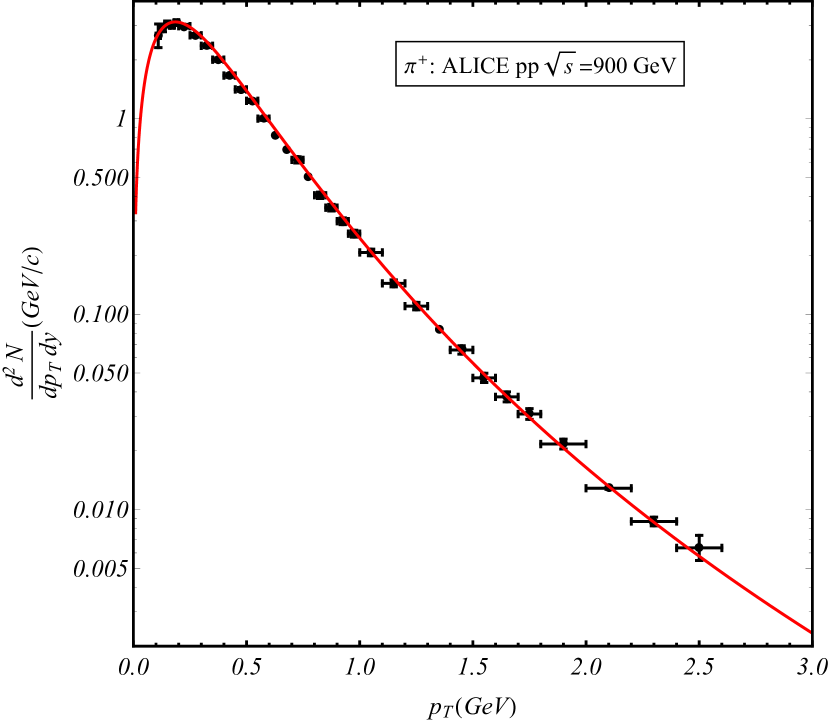
Figure 3: Description of $\pi^{+}$ spectrum provided in Ref. alicepi using Eq. (15). The parameter values are: $q=0.8795\pm 0.004391$, $T=0.0883\pm 0.002957$ GeV, $R=3.873\pm 0.1063$ fm, $\chi^{2}$/NDF = 2.667/30.

IV Summary, outlook, and conclusion

To summarize, we have derived a novel nonadditive bosonic single-particle distribution by extremizing nonadditive entropy. By utilizing the methods of nonadditive statistical mechanics to study a single-mode simple harmonic oscillator, we avoid diverging results reported in previous works. The nonadditive distribution well describes spectra of the bosonic particles like the pions and kaons produced in high-energy collisions, while the conventional Bose-Einstein spectrum deviates from experimental data at around $p_{\text{T}}\sim$ 0.5 GeV. The bosonic distribution in Eq. (15) approaches the conventional Bose-Einstein distribution in the limit $q\rightarrow 1$. The factorization approximation of the distribution in high-energy limit ($\epsilon_{p}\gg T,~{}\Lambda$) results in the classical nonadditive distribution.

A single-particle distributions similar to (but not exactly the same as) Eq. (15) also appears in the thermal Green’s function in nonadditive statistics AbeEPJB . However, Ref. AbeEPJB considers a different definition of mean values given by escort distribution and a proper comparison can be made only when such a definition is considered in the present work as well. Using the escort probabilities, it is possible to evaluate thermodynamic quantities of a system of harmonic oscillators of different frequencies IshiharaEPJB ; Ishiharaarxiv . It will be interesting to study if the result of the present work can be reproduced within the framework of these references. It is also worth mentioning that the classical limit of Eq. (15) appears as the stationary solution of the nonadditive Boltzmann transport equation that considers a generalization of the ‘molecular chaos hypothesis’ wilkosada .

Extension to fermions may be performed by considering a fermionic oscillator. The Hilbert space of a fermionic harmonic oscillator contains only two states ($|0\rangle$ and $|1\rangle$). By using the BG partition function of a single-mode fermionic oscillator, given by $Z_{\text{G}}(\beta^{\prime})=1+\exp(-\beta^{\prime}\epsilon_{p})$, in Eq. (12), one may be able to derive that the fermionic distribution is given by $\left(1+\frac{1-q}{qT}(\epsilon_{p}-\Lambda)\right)^{-\frac{1}{1-q}}$ which in the limit $q\rightarrow 1$ (BG limit) yields $\exp(-\beta(\epsilon_{p}-\Lambda)$. Since $\exp(\beta\Lambda)=Z_{\text{G}}(\beta)^{-1}$, the nonadditive distribution for fermions approach the Boltzmann-Gibbs Fermi-Dirac distribution in the limit $q\rightarrow 1$. Given the bosonic distribution in Eq. (15), it may be possible to estimate thermal mass and express strong coupling $\alpha_{\text{s}}$ in terms of temperature and the entropic parameter $q$ SukanyaEPJC . Such a parameterization of the strong coupling may be utilized to improve the description of $\alpha_{\text{s}}$ at low energies JavidanEPJA . The present work may also lead to the formulation of a nonadditive equation of state that may be employed in studies of nonlinear waves inside Quark-Gluon Plasma tbepjc1 , or studying stellar matter deppmanepja .

References

- (1) K. Aamodt et al. (ALICE Collaboration), Eur. Phys. J C 71, 1655 (2011).
- (2) V. Khachatryan et al. (CMS collaboration), Phys. Rev. Lett. 105, 022002 (2010).
- (3) S. Acharya et al. (ALICE collaboration), Phys. Rev. C 97, 024615 (2018).
- (4) M. D. Azmi, T. Bhattacharyya, J. Cleymans, and M. Paradza, J. Phys. G 47, 045001 (2020).
- (5) M. Rybczyński and Z. Włodarczyk, Eur. Phys. J. C 74, 2785 (2014).
- (6) C. Tsallis, J. Stat. Phys. 52, 479 (1988).
- (7) G. Wilk and Z. Włodarczyk, Phys. Rev. Lett. 84, 2770 (2000).
- (8) G. Wilk and Z. Włodarczyk, Phys. Rev. C 79, 054903 (2009).
- (9) A. Deppman, E. Megías, and D. P. Menezes, Phys. Rev. D 101, 034019 (2020).
- (10) M. Rybczyński, G. Wilk, and Z. Włodarczyk, Phys. Rev. D 103, 114026 (2021).
- (11) A. Lavagno, Phys. Lett. A 301, 13 (2002).
- (12) T. Osada and G. Wilk, Phys. Rev. C 77, 044903 (2009).
- (13) T. S. Biro and E. Molnar, Eur. Phys. J. A 48, 172 (2012).
- (14) A. S. Parvan and T. Bhattacharyya, Eur. Phys. J. A 56, no.2, 72 (2020).
- (15) T. Bhattacharyya and A. S. Parvan, Eur. Phys. J. A 57, no.6, 206 (2021).
- (16) C. Tsallis, R.S. Mendes, and A.R. Plastino, Physica A 261, 534 (1998).
- (17) E.T. Jaynes, Phys. Rev. 106 (1957) 620.
- (18) M. Abramowitz and I. Stegun, Handbook of Mathematics Functions, Nat. Bur. Stand. Appl. Math. Ser., vol. 55 (U.S. Govt. Printing Office, Washington, DC 1965).
- (19) H. Hasegawa, Phys. Rev. E 80, 011126 (2009).
- (20) J.M. Conroy, H.G. Miller, A.R. Plastino, Phys. Lett. A 374, 4581 (2010)
- (21) S. Abe, Eur. Phys. J. B 9, 679 (1999).
- (22) M. Ishihara, Eur. Phys. J. B 95, 53 (2022).
- (23) M. Ishihara, Eur. Phys. J. Plus 139, 1004 (2024).
- (24) S. Mitra, Eur. Phys. J. C 78(1), 66 (2018).
- (25) K. Javidan, M. Yazdanpanah, and H. Nematollahi, Eur. Phys. J. A 57, 78 (2021).
- (26) T. Bhattacharyya and A. Mukherjee, Eur. Phys. J. C 80, 656 (2020).
- (27) P. H. G. Cardoso, T. N. da Silva, A. Deppman, and D. P. Menezes, Eur. Phys. J. A 53, 191 (2017).