A new type of minimizers in lattice energy and its application
Abstract.
Let and
In this paper, we characterize the following minimization problem
We prove that there exist hexagonal to skinny-rhombic minimizers, which is a novel finding in the literature.
1. Introduction and Statement of Main Results
The fact that chemical elements combine to form crystals, periodic objects where the atoms are arranged in a periodic lattice of points with a limited set of symmetries, has been a basic belief for more than two centuries (Bindi [12]). However, there is still an open largely crystal problem: what are the fundamental mechanisms behind the spontaneous arrangement of atoms into periodic configurations at low temperatures? (Radin [27]). This famous problem, called as ‘Crystallization Conjecture’, was proposed by Radin in 1987, a recent review of this conjecture can be found in Blanc-Lewin [13].
We are particularly interested in two-dimensional crystals. These systems capture many essential features of higher dimensions without the added complexity. Two-dimensional crystals play a crucial role in various physical systems, such as lipid monolayers on the surface of water [17], a monolayer of electrons on the surface of liquid helium, rare-gas clusters [29], colloidal systems in two dimensions [26], and dusty plasmas [25]. For a comprehensive overview of these applications, see Bétermin [1, 2, 3, 5, 9].
A fundamental mathematical and physical model for the Crystallization Conjecture and two-dimensional crystals is given by:
| (1.1) |
The denotes the lattice energy per particle of the crystals, the summation ranges over all the lattice points except the origin . is the background potential of the system and denotes the lattice. For the Riesz potential with , the lattice energy becomes the classical Epstein zeta function, Rankin [28], Cassels [14], Ennola [30] and Diananda [15] proved that the hexagonal lattice is the unique minimizer of the Epstein zeta function up to the action by modular group. For the Gaussian potential with , the lattice energy becomes the classical theta function, and Montogmery [24] proved that the hexagonal lattice still minimize the lattice energy. In fact, Montogmery’s Theorem [24] implies the results of Rankin [28], Cassels [14], Ennola [30] and Diananda [15]. The motivation of these research come from pure interest of number theory, and it turns out these theorems have deep applications in lattice energy.
In this paper, we are interested in the lattice energy of the following difference form:
| (1.2) |
where the potentials are two potentials with simple forms. Mathematically, the problem (1.2) is equivalent to the problem (1.1), but physically, it introduces new insights. For more details on this model and its applications in physics, we refer to Bétermin [3, 8, 9, 10], Bétermin-Petrache[7], Bétermin-Faulhuber-Knpfer [6], and Bétermin-Friedrich-Stefanelli [11]. The problem (1.2) was initiated by the study of difference of Yukawa potential (Bétermin [2]), Lennard-Jones potential (Bétermin [3]), and Morse potential (Bétermin [4]).
In this paper, we consider the potential of the form:
| (1.3) |
Let and be the lattices with unit density in . Define
| (1.4) |
Then the lattice energy (1.2) under potential (1.3) becomes
It is interesting to study the phase transitions of the lattice energy under the potential (1.3). To this end, we prove the following theorem:
Theorem 1.1.
Assume that . Consider the lattice energy:
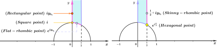
Then, up to the action by modular group, there exists two thresholds , where depends on with bound and is independent of . Specifically, the following holds:
-
(1)
For , the minimizer is , corresponding to a hexagonal lattice.
-
(2)
For , the minimizer is with , corresponding to a skinny-rhombic lattice. Furthermore, as approaches , approaches .
-
(3)
For , the minimizer does not exist.
Bétermin discovered the hexagonal-rhombic-square-rectangular phase transitions of the system under Lennard-Jones potential and Morse potential in [3] and [4], respectively. A rigorous proof of these phase transitions can be found in tri-copolymer systems (Luo-Ren-Wei [18]) and Bose-Einstein condensates (Luo-Wei [19]), respectively. In Theorem 1.1, we uncover a new type of phase transition from hexagonal to skinny-rhombic.
This paper is organized as follows. In Section 2, we introduce the symmetries of the function , such that this problem can be reduced to the fundamental domain. In Section 3, we prove that the minimization problem on the fundamental domain can be reduced to its right boundary. In Section 4, we explain partially the case where the minimizer is the hexagonal point and the methods can be applied to the relevant problems. Finally, in Section 5, we prove Theorem 1.1.
2. Preliminaries
In this section, we collect some basic properties of the theta function along with some useful estimates of Jacobi theta function. We also introduce a group related to the functional . The generators of the group are given by
| (2.5) |
By Definition (2.5), the fundamental domain associated to modular group is
| (2.6) |
The following lemma characterizes the invariance properties of the theta function under the action of the group :
has a close connection to the theta function.
Lemma 2.2 (The relationship between the function and the theta function).
Lemma 2.3 (The invariance of ).
For any , any and , it holds that
The Jacobi theta function is defined as follows:
The classical one-dimensional theta function is given by
| (2.7) |
By the Poisson summation formula, it holds that
| (2.8) |
To estimate bounds of quotients of derivatives of , we denote that
and
| (2.9) | ||||
There are some useful estimates for quotients of 1-d theta functions and their derivatives.
Lemma 2.4 (Luo-Wei [19]).
Assume that . It holds that
-
(1)
if , then
-
(2)
if , then
Remark 2.1.
By Lemma 2.4, for .
Furthermore, the following estimates for higher order derivatives of quotients of 1-d theta functions hold:
3. The transversal monotonicity
We define the vertical line in the upper half-plane as follows:
By the group invariance (Lemma 2.3), one has
| (3.10) |
In this section, we aim to establish the following theorem:
Theorem 3.1.
Assume that . Then for , it holds that
To prove Theorem 3.1, we establish the following monotonicity result:
Proposition 3.1.
Assume that . Then it holds that
Note that Proposition 3.1 implies Theorem 3.1. The rest of this section is devoted to proving Proposition 3.1.
3.1. The estimates
Using the ideas from Bétermin [2] and Luo-Wei [20, 22, 23], we will utilize the exponential expansion of the theta function, such that Theorem 3.1 is reduced to the study of Jacobi theta function.
Based on Lemmas 2.2 and 3.1, we derive the exponential expansion of the function in Lemma 3.2. The proof of Lemma 3.2 is straightforward, hence we omit it.
Lemma 3.2.
We have the following expression of : for , it holds that
By Lemma 3.2, we have:
Lemma 3.3.
We have the following identity for the partial -derivative of the function :
where
| (3.11) | ||||
and
| (3.12) | ||||
Lemma 3.4.
Assume that . Then for , it holds that
To explain Lemma 3.4, we aim to illustrate that acts as the major term, which is positive, while represents an error term that does not change the sign of the whole expression. Based on (3.11) and (3.12), we will provide a deformation of and an upper bound for in the following lemma:
Lemma 3.5.
Assume that . Then for , it holds that
-
(1)
Deformation of
-
(2)
Upper bound for
We will divide the proof of Lemma 3.4 into three cases, where Case A: , Case B: and Case C: , which will be presented separately in the next three subsections.
3.2. Case A of Lemma 3.4:
In this subsection, we shall prove that
Lemma 3.6.
Assume that , then for , it holds that
-
(1)
The lower bound function of
-
(2)
The upper bound function of
-
(3)
Proof.
By Lemmas 3.5, 2.4 and 2.5, one has
| (3.13) | ||||
Notice that and are decreasing as . Then as , one has
| (3.14) |
Notice that for , we have
| (3.15) |
Then, there holds that
| (3.16) |
Therefore, (3.13)-(3.16) yield item (1). By Lemmas 3.5 and 2.4, one gets
| (3.17) | ||||
Note that implies . Then for and , by (3.15), (LABEL:3.2eq5), along with the monotonicity of and , item (2) is deduced. Items (1) and (2) yield item (3). ∎
3.3. Case B of Lemma 3.4:
In this subsection, we shall prove that
Lemma 3.7.
Suppose , then for , it holds that
-
(1)
The lower bound function of
-
(2)
The upper bound function of
-
(3)
3.4. Case C of Lemma 3.4:
In this subsection, we shall prove that
Lemma 3.8.
Assume that , and . Then for , it holds that
-
(1)
Lower bound of
-
(2)
Upper bound of
-
(3)
4. Minimization on the vertical line
Theorem 4.1.
Assume that . Then, for , up to the action by the modular group,
Regarding to , it is known that
Proposition 4.1 (Luo-Wei [22]).
For , up to the modular group, then
Proposition 4.2.
Assume that . Then, up to the action by the modular group,
This proof of Proposition 4.2 is based on Propositions 4.3 and 4.4 (an illustration the proof can be found in Figure 2).
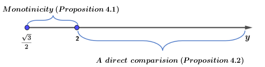
Proposition 4.3.
Suppose that . Then for , it holds that
For , we use a direct method as follows:
Proposition 4.4 (A direct comparison).
Suppose that . Then for , it holds
4.1. Proof of Proposition 4.3
By Proposition 3.4 of Bétermin [3]:
and to prove Proposition 4.3, it suffices to prove Lemma 4.1. In this subsection, we aim to prove that
Lemma 4.1.
Assume that . Then for ,
To better illustrate the proof of Lemma 4.1, we denote that
| (4.19) | ||||
Using the expression of given by (1.4), we give the expression of in the following lemma. The proof of this lemma is straightforward and thus omitted.
Lemma 4.2 (The expression of ).
In view of the expression provided in Lemma 4.2, we first provide the lower bound estimates of .
Lemma 4.3 (The lower bound estimates).
For , it holds that
-
(2)
-
(3)
-
(4)
-
(1)
The following results were derived in Luo-Wei ([20]).
Lemma 4.4 (Luo-Wei [20]).
For , it holds that
-
(1)
-
(2)
where
and and each is expressed as follows
Numerically, and
Next, we provide upper bound of .
Lemma 4.5 (Upper bound of ).
For , it holds that
-
(1)
-
(2)
where . Here each is small and expressed by
and
Numerically, , and
Proof.
Since the proofs of the two items in Lemma 4.5 are similar, we provide the proof for item (1) only to avoid repetition. For simplicity, we denote:
| (4.20) | ||||
Then, by (4.19), the sum can be divided into the following four parts:
| (4.21) |
Next, we shall calculate the four parts respectively. Using (4.20), one has
| (4.22) | ||||
and
| (4.23) | ||||
Similarly,
| (4.24) | ||||
and
| (4.25) | ||||
4.2. Proof of Proposition 4.4
We first give the exponential expansion of .
Lemma 4.6.
For , we have the following expression of
In view of Lemma 4.6, to better demonstrate the proof of Proposition 4.4, we will decompose the expression . We denote that
| (4.30) | ||||
and
| (4.31) | ||||
By (4.30) and (4.31), we further denote that
| (4.32) |
Thus, by Lemma 4.6 and (4.30)-(4.32), we have
| (4.33) |
Lemma 4.7.
Assume that , it holds that
To prove Lemma 4.7, we aim to show that the term
is positive and serves as the principal term, while the term
is significantly smaller in comparison when when . Given the complexity of this problem, our proof will be divided into two cases: and .
Lemma 4.8.
Assume that . Then
-
(1)
-
(2)
-
(3)
-
(4)
Proof.
Recall that In the following lemma, we will provide an lower bound for to prove (1) of Lemma 4.8.
Lemma 4.9.
Assume that then . We split it into four items.
-
(1)
-
(2)
-
(3)
-
(4)
Proof.
Before providing an upper bound function of , we denote that
| (4.38) | ||||
Lemma 4.10 (An upper bound function of ).
Assume that . Then
-
(1)
-
(2)
-
(3)
-
(4)
-
(5)
Trivially,
Proof.
We then give the proof of item (2) in Lemma 4.8.
Lemma 4.11.
Assume that . Then it holds that
-
(1)
If , then
-
(2)
If , then
Proof.
For simplicity, we denote that
| (4.41) |
A direct calculation shows that
| (4.42) |
As , by (4.41), one has
| (4.43) |
By (2.8) and (4.42)-(4.43), one has
| (4.44) |
Given that , by (2.7), one has
| (4.45) |
Then (4.43)-(4.45) yield item (1). By (4.39), one has
| (4.46) |
Then for , by (4.42) and (4.46), we have
| (4.47) |
By (4.39), one has
| (4.48) | ||||
and
| (4.49) |
Here, since , one has
| (4.50) |
and
| (4.51) |
Then for , by (4.48)-(4.51), one has
| (4.52) |
As , by (2.7), one has
| (4.53) |
Then combining (4.47) with (4.52)-(4.53), we obtain item (2).
∎
Finally, we provide the proof Lemma 4.7 for . It is stated as follows:
Lemma 4.12.
Assume that . Then
-
(1)
Lower bound estimate of the major term.
-
(2)
An auxiliary estimate about the error term.
-
(3)
Comparison of the error term with the major term.
-
(4)
Proof.
Note that . By Lemmas 4.13 and 4.10, one has
which yields item (1). By Lemma 4.11 and (2.8), we have
| (4.54) | ||||
Item (2) follows by (LABEL:4.3lemma2error) and the conditions that Combining item (1) with , one has
| (4.55) | ||||
Then, (4.55) and item (2) together yield item (3). Items (1) and (3) yield item (4). ∎
For simplicity, we denote that
The following lemma provides the bounds used in Lemma 4.12.
Lemma 4.13.
Assume that . Then
-
(1)
-
(2)
-
(3)
-
(4)
-
(5)
Numerically, ,
Proof.
We provide the bounds before the proof. Noting that , we calculate directly that
| (4.56) | ||||
and
| (4.57) | ||||
(1). For , by (2.8), (4.30) and (4.56), one has
(2). For , by (4.30) and (4.39), one has
| (4.58) | ||||
which yields item (2).
5. Proof of Theorem 1.1
We start with a nonexistence result.
Proposition 5.1.
Assume that , Then for , does not exist.
Proof.
We observe that
Lemma 5.1.
Assume that . Then for , it holds that
To prove Lemma 5.1, we will seek an appropriate lower bound for and an upper bound for . To state the proof clearly, we decompose into several parts. We denote that
Then
| (5.64) |
Lemma 5.2.
Assume that and .
-
(1)
If then
-
(1)
-
(2)
-
(1)
-
(2)
If , then
-
(1)
-
(2)
-
(1)
-
(3)
Proof.
(1). Combining (2.7) and , one has
| (5.65) | ||||
For and , similar to the analysis of positiveness of and in Lemma 4.9, one can get and . Then, by (5.64) and (5.65), we obtain the lower bound estimate of . Similar to the proof of item (2) of Lemma 4.8, using (2.7), (2.8) and Lemma 4.11, we can get an upper bound estimate of .
(2). As , for , by (2.8), one has
| (5.66) | ||||
Similar to the analysis of the positiveness of and in Lemma 4.13, one gets and Thus, by (5.64), (5.66) and the positiveness of and , we get the estimate for . Similar to the proof of item (2) of Lemma 4.8, we get the upper bound estimate of . Items (1) and (2) yield item (3). ∎
With the previous preparation, we are ready to prove our main theorem.
Case 1: By Theorems 3.1 and 4.1, we obtain that, up to the action by the modular group,
| (5.67) |
Therefore, we introduce and define that
Then by Proposition 5.1 and (5.67), . The threshold varies with . For example, when , and when
Case 2: When , by Theorem 3.1 and (5.62), the minimizer always exists. Furthermore, by Theorem 3.1 and the definition of in (1.4), the minimizer is , corresponding the skinny-rhombic lattice. A numerical simulation can be found in Figure 3. Furthermore, the monotonicity result in Luo-Wei-Zou [21] implies that when approaches , approaches .
Case 3: It follows by Proposition 5.1.
Acknowledgements. The research of S. Luo is partially supported by the National Natural Science Foundation of China (NSFC) under Grant Nos. 12261045 and 12001253, and by the Jiangxi Jieqing Fund under Grant No. 20242BAB23001.
References
- [1] L. Bétermin and P. Zhang, Minimization of energy per particle among Bravais lattices in Lennard-Jones and Thomas-Fermi cases, Commun. Contemp. Math., 17(6) (2015), 1450049.
- [2] L. Bétermin, Two-dimensional theta functions and crystallization among Bravais lattices, SIAM Journal on Mathematical Analysis, 48(5) (2016), 3236-269.
- [3] L. Bétermin, Local variational study of 2d lattice energies and application to Lennard-Jones type interactions, Nonlinearity, 31(9) (2018), 973-4005.
- [4] L. Bétermin, Minimizing lattice structures for Morse potential energy in two and three dimensions, Journal of Mathematical Physics, 60(10) (2019), 102901.
- [5] L. Bétermin and M. Petrache, Dimension reduction techniques for the minimization of theta functions on lattices, Journal of Mathematical Physics, 58 (7) (2017), 071902.
- [6] L. Bétermin, M. Faulhuber and H. Knpfer, On the optimality of the rock-salt structure among lattices with charge distributions, Mathematical Models and Methods in Applied Sciences, 31 (2): 293-325, 2021.
- [7] L. Bétermin and M. Petrache, Optimal and non-optimal lattices for non-completely monotone interaction potentials, Analysis and Mathematical Physics, 9 (4): 2033-2073, 2019.
- [8] L. Bétermin, On energy ground states among crystal lattice structures with prescribed bonds, Journal of Physics A, 54(24): 245202, 2021.
- [9] L. Bétermin, Effect of periodic arrays of defects on lattice energy minimizers. Ann. Henri Poincaré 22 (2021), no. 9, 2995-3023.
- [10] L. Bétermin, L.De Luca and M. Petrache, Crystallization to the Square Lattice for a Two-Body Potential, Arch. Rational Mech. Anal., 240, 987-1053 (2021).
- [11] L. Bétermin, M. Friedrich and U. Stefanelli, Letters in Mathematical Physics, Lattice ground states for embedded-atom models in 2D and 3D, Volume 111, article number 107, (2021).
- [12] L. Bindi, What Are Quasicrystals and Why They Are so Important? In: Natural Quasicrystals. SpringerBriefs in Crystallography. Springer, Cham, 2020.
- [13] X.Blanc and M. Lewin, The crystallization conjecture: a review, EMS Surv. Math. Sci. 2 (2015), no. 2, pp. 255-306.
- [14] J. W. S. Cassels, On a problem of Rankin about the Epstein zeta function, Proc. Glasgow Math. Assoc., 4 (1959), 73-80. (Corrigendum, ibid. 6 (1963), 116.)
- [15] P. H. Diananda, Notes on two lemmas concerning the Epstein zeta-function, Proc. Glasgow Math. Assoc. 6 (1964), 202-204.
- [16] K. Deng and S. Luo, Minimizing Lattice ennergy and hexagonal crystallization,
- [17] V. M. Kaganer, H. Möhwald, and P. Dutta, Structure and phase transitions in Langmuir monolayers, Rev. Mod. Phys., 71, 779, 1999.
- [18] S. Luo, X. Ren and J. Wei, Non-hexagonal lattices from a two species interacting system, SIAM J. Math. Anal., 52(2) (2020), 1903-1942.
- [19] S. Luo and J. Wei, On minima of sum of theta functions and application to Mueller-Ho conjecture, Arch. Ration. Mech. Anal., 243 (2022), no. 1, 139-199.
- [20] S. Luo and J. Wei, On minima of difference of theta functions and application to hexagonal crystallization, Math. Ann., 387 (2023), no. 1-2, 499-539.
- [21] S. Luo, J. Wei and W. Zou, On universally optimal lattice phase transitions and energy minimizers of completely monotone potentials, arXiv:2110.08728.
- [22] S. Luo and J. Wei, On lattice hexagonal crystallization for non-monotone potentials, J. Math. Phys., 65(2024), no. 7, Paper No. 071901, 28 pp.
- [23] S. Luo and J. Wei, On a variational model for the continuous mechanics exhibiting hexagonal to square phase transitions, arxiv:2312.02497.
- [24] H. Montgomery, Minimal theta functions, Glasgow Math. J., 30 (1988), 75-85.
- [25] V. Nosenko, K. Avinash, J. Goree, and B. Liu, Nonlinear Interaction of Compressional Waves in a 2D Dusty Plasma Crystal, Phys. Rev. Lett., 92, 085001, 2004.
- [26] F. M. Peeters and Xiaoguang Wu, Wigner crystal of a screened-Coulomb-interaction colloidal system in two dimensions, Phys. Rev. A,35, 3109, 1987.
- [27] C. Radin, low temperature and the origin of crystallization symmetry, International Journal of Modern Physics B, Vol. 01, No. 05n06, pp. 1157-1191 (1987).
- [28] R. A. Rankin, A minimum problem for the Epstein zeta function, Proc. Glasgow Math. Assoc., 1 (1953), 149-158.
- [29] P. Schwerdtfeger, N. Gaston, R. P. Krawczyk, R.f Tonner, and G. E. Moyano, Extension of the Lennard-Jones potential: Theoretical investigations into rare-gas clusters and crystal lattices of He, Ne, Ar, and Kr using many-body interaction expansions, Phys. Rev. B, 73, 064112, 2006.
- [30] Viekko Ennola, A lemma about the Epstein zeta function, Proc. Glasgow Math. Assoc., 6 (1964), 198-201.