On M87^∗ and SgrA^∗ Observational Constraints of Dunkl Black Holes

Abstract

In this work, we investigate the optical properties of a new black hole recently obtained from the Dunkl operator formalism involving a relevant parameter denoted by $\xi$. Concretely, we first investigate the shadows, the Lyapunov exponents of unstable nearly bound orbits and the spherically infalling accretion behaviors in terms of such a parameter. Then, we examine the effect of this parameter on the Dunkl black hole deflection angle in vacuum and medium backgrounds by manipulating the Gauss-Bonnet theorem. Exploiting the M87^∗ and SgrA^∗ optical bonds, we provide strong constraints on $\xi$ via the falsification mechanism.

1 Introduction

Recently, the physics of black holes has attracted a great deal of interest via various theoretical and empirical investigations including the Even Horizon Telescope (EHT) collaborations and the detection of gravitational waves [1, 2, 3]. Theoretically, the thermodynamics[4, 5, 6, 7, 8, 9, 10, 11, 12, 13, 14, 15, 16, 17, 18] and the optic[19, 20, 21, 22] are the most studied subjects by considering gravity theories in various geometric backgrounds such as the cosmological spacetimes and the Universe dark sectors. In connection with the phase transitions, the anti de Sitter (AdS) spaces have been placed in the center of such investigations [23, 24, 16]. Transforming the cosmological constant into pressure, several phase transitions, such as the Hawking-Page one, have been investigated in the presence of ordinary and non-ordinary parameters. Different scenarios, including the criticality and the stability properties, have been explored to inspect the thermodynamic behaviors of the AdS black holes. Various impacts as the spacetime dimension, the dark matter and the dark energy have been extensively studied over the last few years. It has been found certain significant modifications depending on the extra parameters in arbitrary dimensions.

With reference to the EHT collaborations, the light behaviors near black holes have been largely investigated. The shadow configurations, considered as the indirect test of the even horizon, have been approached by considering different gravity theories including the modified ones [25, 26]. These activities are supported and encouraged by the imaging of the supermassive M87^∗ black hole. This has been confirmed by the image of the SgrA^∗ black hole. These observational findings have shown the real behaviors of the underlying physics of black holes [27, 28, 29, 30, 31]. Motivated by such an empirical aspect, the shadows of several black holes have been elaborated. Concretely, different sizes and shapes have been obtained by combing the general relativity (GR) and the hamiltonian formalism techniques. Precisely, the photons near black holes have been approached by establishing the associated equations of motion via numerical computation methods. Circles and deformed ones have been obtained depending on the absence or the presence of certain black hole parameters[32, 33, 34, 35, 36]. The size and the shape deformations have been examined by help of the geometrical observables using appropriate numerical simulations. Alternatively, the deflection of light rays in curved geometries have been also investigated in connection with the black hole physics. Considering a static spherically symmetric solutions, the light deflection angles by various black holes have been computed and inspected in the presence of non trivial parameters. The Gauss-Bonnet theorem is considered as the most used method to provide interesting results on the deflection angle [37, 38, 39, 40, 41, 42, 43]. This computing road, proposed first by Gibbons and Werner [44, 45] in the context of the optical geometries for asymptotically flat backgrounds, has been exploited to explore a bridge to thermodynamics [46, 47]. In particular, it has been shown that this quantity could provide data on the phase transitions in the AdS black holes. Based on the elliptic functions, the phase structure of the charged AdS black holes has been studied from thermal variations of the deflection angle. Precisely, it has been suggested that the large black hole/small black hole transition can occur naturally at specific values of the deflection angle.

More recently, the empirical activities provided by the EHT collaborations have been exploited to show the validity and the viability of certain modeled black holes including the non-Kerr solutions. Concretely, the M87^∗ and the SgrA^∗ black hole measurements could provide strong conditions for the proposed models. More precisely, the EHT bounds on the shadows have been investigated to put constraints on the black hole parameters including the charge [48, 49, 31, 36, 50].

In relation to the EHT observational findings, moreover, certain constraints on the deflection angle in the dark matter backgrounds have been studied in order to unveil information on the underlying interactions. Among others, it has been shown that the deflection angle can supply an alternative road to detect the dark matter going beyond the black hole shadow investigations [51].

Motivated by such activities, we investigate the optical behaviors of a new black hole recently obtained in [52]. The latter will be called Dunkl black hole derived from the implementation of the Dunkl operator formalism in the gravity calculations. The resulting model involves a relevant parameter denoted by $\zeta$ being the center of the present investigation. Precisely, we first discuss the shadow, the Lyapunov exponents of unstable nearly bound orbits and the spherically infalling accretion behaviors in terms of such a parameter. After that, we study the Dunkl black hole deflection angle in vacuum and medium backgrounds by manipulating the Gauss-Bonnet theorem. Employing the M87^∗ and SgrA^∗ optical bonds, we supply strong constraints on $\xi$ via the falsification mechanism.

The organization of this paper is as follows. In section 2, we reconsider the study of the Dunkl black hole. Section 3 fournishes the computations dealing with the shadows and the deflection angle. In section 4, we exploit the EHT bands to determine certain constraints of the Dunkl parameter $\xi$ from optical computations. In this work, the natural units $G=c=1$ have been used.

2 Dunkl black hole

In this section, we reconsider the study of the Dunkl black hole recently proposed in [52]. In particular, we provide the essentials on the associated solutions from the Dunkl operator formalism combined with gravity computations. For simplicity reasons, we deal with the spherical solution via the following line element

$$ds^{2}=-f(r)dt^{2}+\frac{1}{f(r)}dr^{2}+r^{2}\left(d\theta^{2}+\sin^{2}\theta d\phi^{2}\right)$$ (1)

where the metric function $f(r)$ carries physical data on the black holes. The coefficients of such a radial function parametrizes a space called the moduli space. Certain regions of such a space can provide results that could be corroborated by EHT empirical findings. In the present work, the moduli space will be approached via a new relevant parameter derived naturally from the Dunkl operator formalism being largely investigated in connection with various mathematical and physical subjects [53, 54, 55, 56]. It has been remarked that the Dunkl derivative is a generalization of the ordinary derivative in the Euclidean spaces involving reflection operations. These generalised derivatives introduced by C. F. Dunkl rely on reflection symmetries associated with non-trivial mathematical structures including the Coxeter groups and the root systems [53, 57]. In Cartesian geometry, the general expression of the Dunkl operators take the following form

$$D_{x_{i}}=\dfrac{\partial}{\partial x_{i}}+\dfrac{\alpha_{i}}{x_{i}}(1-\mathcal{R}_{i})\quad,\quad i=0,1,2,3$$ (2)

where one has used $\alpha_{i}=\left(0,\alpha_{1},\alpha_{2},\alpha_{3}\right)$ $(\alpha_{i}>-1/2)$ being the Dunkl parameters. $\mathcal{R}_{i}=\left(0,\mathcal{R}_{1},\mathcal{R}_{2},\mathcal{R}_{3}\right)$ denote the parity operators[54, 55, 56]. Combining the Einstein equation and the Dunkl operator formalism, a deformed Schwarzschild spacetime resulting from the gauge theory of gravity in the presence of cosmological constant has been constructed [52]. For a vanishing cosmological constant scenario, the metric function $f(r)$ has been found to be

$$f(r)=\frac{1}{\left(1+\zeta\right)}-2M\,r^{\frac{1}{2}\left(1-\sqrt{9+8\zeta}\right)}\,,$$ (3)

Here, $M$ denotes the black hole mass, and $\zeta$ is the Dunkl parameter where one has used $\zeta=\sum_{i=1}^{3}\alpha_{i}\left(1-\mathcal{R}_{i}\right)\left(1+\alpha_{i}\left(1-\mathcal{R}_{i}\right)\right)$. This parameter being relevant in the present investigation enlarges the ordinary moduli space of the neutral black holes without rotations. It has been revealed that the associated geometrical aspects have been corrected by such a Dunkl parameter $\zeta$. To disclose some pieces of information about the Dunkl parameter $\zeta$ impact, the embedding diagram of such a black hole within different values of the Dunkl parameter $\zeta$ is illustrated in Fig.1.

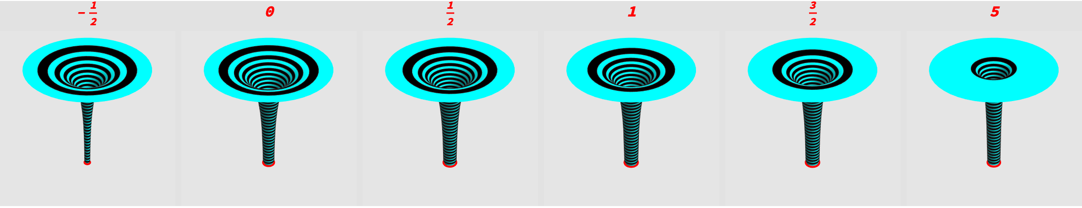
Figure 1: Embedding diagram within different values of the correction parameter $\zeta$, with $M=1$.

Considering the event horizon (red circle), it decreases for negative values of $\zeta$, while for the positive ones, the event horizon increases to reach the value $\zeta=1.59$ then it decreases. In addition, the Schwarzschild black hole is known to have a true physical singularity at $r=0$ and a coordinate singularity at $r=2M$. We now investigate whether the presence of the Dunkl parameter affects the existence of these singularities or it can play a role in regularizing the black hole at $r=0$. To do so, a more comprehensive description of such a black hole spacetime is needed. We recall the Kretschmann invariant, which is a scalar quantity characterizing the curvature of spacetime at a specific point. It is defined as a combination of the Riemann tensor components

$$\mathcal{K} = R_{abcd}R^{abcd},$$

$$= \frac{4\left(\zeta^{2}+2(\zeta+1)^{2}\left(2\zeta(\zeta+4)-\sqrt{8\zeta+9}+9\right)M^{2}r^{1-\sqrt{8\zeta+9}}+4\zeta(\zeta+1)Mr^{\frac{1}{2}-\frac{1}{2}\sqrt{8\zeta+9}}\right)}{(\zeta+1)^{2}r^{4}}\,.$$

In Fig.2, we depict the behavior of such a quantity in terms of the radial coordinate $r$ for various ranges (positive/negative) of the Dunkl parameter $\zeta$.

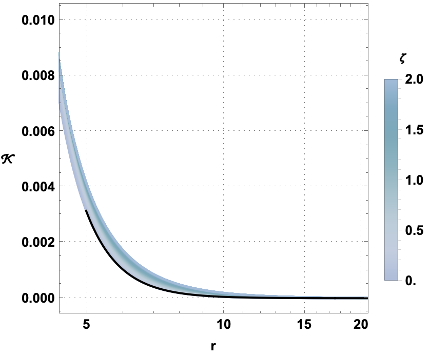
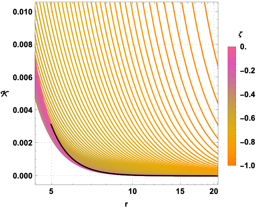
Figure 2: Profile of the embedding diagram within different values of the correction parameter $\zeta$. Left: positive range and Right: negative range. The solid black line corrreponds to the Schwarzschild solution associated with $\zeta=0$.

It has been observed, from the left panel associated with the positive values of $\zeta$, that the Kretschmann number increases as $\zeta$ grows. This indicates that spacetime is significantly curved, leading to deviations from the flat spacetime for the high values of the Dunkl parameter. For negative ranges of $\zeta$, however, two distinctive schemes appear. For $\zeta\leq-0.4$, the Kretschmann quantity decreases as the absolute value of $\zeta$ increases, while for $\zeta\geq-0.4$ the situation is inverted.

In the present work, we would like to go beyond such geometrical aspects by investigating the optical behaviors via the shadows, and the deflection angle computations and other related discussions. This study could bring data on the acceptable regions of the extended moduli space by exploiting the known black hole empirical studies. The forthcoming sections will concern the geometric engineering of the certain optical aspects of the Dunkl black hole via real curves and their contacts with the EHT empirical findings.

3 Optical behaviors of the Dunkl black hole

In this section, we conduct an examination of specific optical properties associated with the Dunkl black hole, focusing on certain aspects such as the shadows and the light deflection angle behaviors in various contextual backgrounds.

3.1 Shadows of the Dunkl black hole

First, we would like to appraoch the shadow behavior of the Dunkl black hole. Precisely, we exploit the Hamilton-Jacobi scenario needed to elaborate the equations of motion of photons near such a black hole. To start, we consider null geodesic equations

$$\mathcal{H}=\frac{1}{2}g^{\mu\nu}p_{\mu}p_{\nu}=0$$ (5)

where the quantity $g^{\mu\nu}$ represents the associated black hole metric given in terms of the line element $ds^{2}=g^{\mu\nu}dx_{\mu}dx_{\nu}.$ In the equatorial plane defined by $\theta=\pi/2$, Eq.(5) can be reduced to

$$\frac{1}{2}\left[-\frac{p_{t}^{2}}{f(r)}+f(r)p_{r}^{2}+\frac{p^{2}_{\phi}}{r^{2}}\right]=0.$$ (6)

In these computations, two constants of motion appear naturally. They are the energy $\mathcal{E}$ and the angular momentum $\mathcal{J}$ of the photon given by

$$\mathcal{E}=-\frac{\partial\mathcal{H}}{\partial\dot{t}}\,,\qquad\mathcal{J}=\frac{\partial\mathcal{H}}{\partial\dot{\phi}}.$$ (7)

Here, one has used the following equations

$$\dot{t}=\frac{\partial H}{\partial p_{t}}=-\frac{p_{t}}{f(r)}\,,\qquad\dot{\phi}=\frac{\partial H}{\partial p_{\phi}}=\frac{p_{\phi}}{r^{2}}\,,$$ (8)

where the over dot is the derivative with respect to the affine parameter $\tau$. Using the radial momentum $p_{r}$ via the relation

$$\dot{r}=\frac{\partial H}{\partial p_{r}}=p_{r}f(r)$$ (9)

the effective potential satisfies

$$V_{\text{eff}}(r)+\dot{r}^{2}=0.$$ (10)

This gives

$$V_{\text{eff}}(r)=f(r)\left[\frac{\mathcal{J}^{2}}{r^{2}}-\frac{\mathcal{E}^{2}}{f(r)}\right]=\frac{\mathcal{J}^{2}\left(\frac{1}{\zeta+1}-2Mr^{\frac{1}{2}-\frac{1}{2}\sqrt{8\zeta+9}}\right)}{r^{2}}-\mathcal{E}^{2},$$ (11)

where, in the first line, $f(r)$ denotes the metric function given by Eq.(3). Before going ahead, we illustrate the effective potential in the left panel of Fig.3. It is straightforward to demonstrate that the effective potential for the Dunkel-Schwarzschild black hole reaches its maximum at the critical radius $r_{c}$

$$r_{c}=\left(\frac{\sqrt{8\zeta+9}-3}{4\zeta(\zeta+1)M}\right)^{-\frac{2}{\sqrt{8\zeta+9}-1}}.$$ (12)

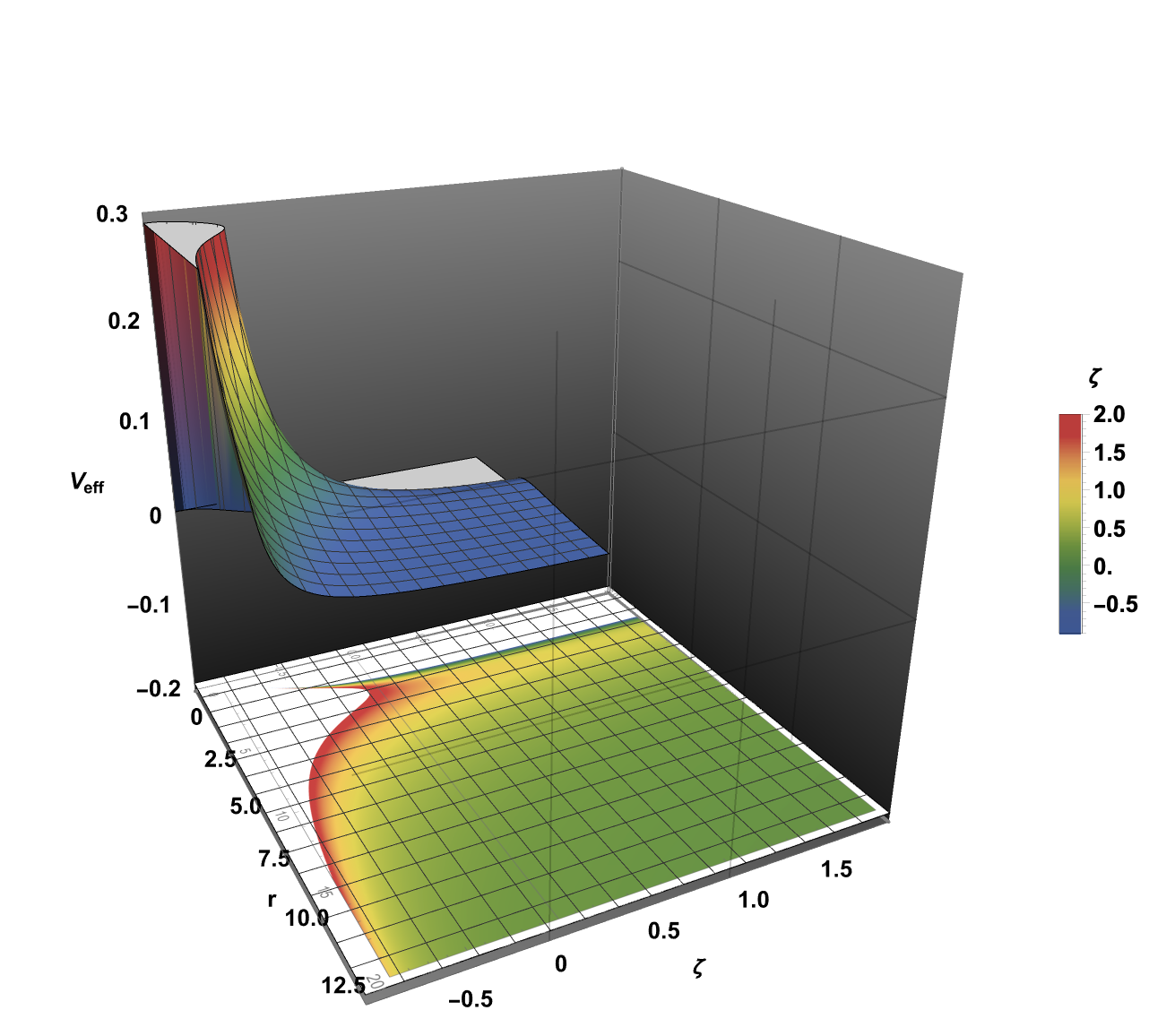
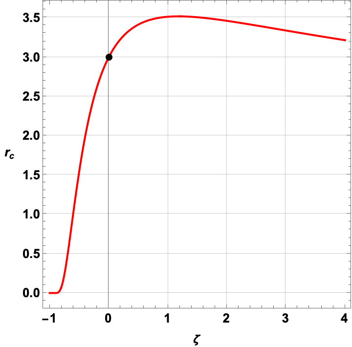
Figure 3: Left: Effective potential by varying the correction parameter $\zeta$. We have set $\mathcal{E}=0.01$ and $\mathcal{J}=1$. Right: Critical radius $r_{c}$ in terms of the Dunkl parameter $\zeta$, with $M=1$.

For the Schwarzschild solution, the effective potential $V_{eff}$ for a photon reaches its maximum at $r=3M$, indicating an unstable circular orbit, as $r$ approaches infinity. The effective potential asymptotes to a constant value. As shown in both panels of Fig.3, as the parameter $\zeta$ increases, the critical radius $r_{c}$ initially rises, reaching a peak around $\zeta=1.18$, before it starts to decrease. This behavior suggests that as the Dunkl parameter grows, the size of the unstable circular orbits initially expands, then it contracts. The photon orbits which are associated with the maximum effective potential are circular and unstable. These unstable circular orbits define the boundary of the black hole apparent shape and can be determined by maximizing the effective potential required by

$$V_{\text{eff}}(r_{c})=0,\quad\text{ and }\left.\frac{\partial V_{\text{eff}}(r)}{\partial r}\right|_{r=r_{c}}=0.$$ (13)

The motion of photons in the Dunkl spacetime is governed by Eqs.(8)-(10). The behavior of photons near the black hole is characterized by two impact parameters, depending on the constants of motion. For general orbits around the black hole, these impact parameters are given by

$$\xi=\frac{L}{E},\qquad\text{ and }\qquad\eta=\frac{\kappa}{E^{2}},$$ (14)

where $\kappa$ is a separating constant where $L$ and $E$ are constants of motion. They are needed to visualize the shadow geometries in four dimensions. To obtain an elegant representation, however, one could use the celestial coordinates $(X,Y)$ representing all projections of the spherical photon orbits [58, 59]. They read as

$$X = -r_{o}\frac{p^{(\phi)}}{p^{(t)}},$$ (15)

$$Y = r_{o}\frac{p^{(\theta)}}{p^{(t)}}.$$ (16)

where $r_{o}$ denotes the distance of the observer from the black hole[60, 35]. Precisely, they are given by

$$\small X = \lim_{r_{{}_{o}\rightarrow+\infty}}\left(-r^{2}_{o}\sin\theta_{o}\frac{d\phi}{dr}\right),$$ (17)

$$Y = \lim_{r_{{}_{o}\rightarrow+\infty}}\left(r^{2}_{o}\frac{d\theta}{dr}\right)$$ (18)

where $\theta_{o}$ is the angle of the inclination between the observer line of sight and the axis of the black hole rotation. Instead of giving an analytic discussion, we use a numerical one by varying the Dunkl parameter $\zeta$. Fig.(4) presents the shadows as a function of such a relevant parameter $\zeta$ in the present work.

Figure 4: Shadows for different values of the correction parameter $\zeta$.

It follows from this figure that $\xi$ can be interpreted as a geometric deformation parameter controlling the involved sizes. Precisely, the size increases by increasing $\xi$ being a relevant free parameter. However, the empirical findings could be exploited to impose constraints on such a parameter needed to predict certain accepted physical ranges. Further, one utilizes the numerical backward ray-tracing approach to analyze the black hole shadows [61]. This technique provides a visual representation of the shadow extent within the lensing ring. In the following tetrad

$$e_{(t)}= \left.\frac{1}{\sqrt{-g_{tt}}}\partial_{t}\right|_{(r_{0},\theta_{0})},e_{(r)}= \left.-\frac{1}{\sqrt{g_{rr}}}\partial_{r}\right|_{(r_{0},\theta_{0})},e_{(\theta)}= \left.\frac{1}{\sqrt{g_{\theta\theta}}}\partial_{\theta}\right|_{(r_{0},\theta_{0})},e_{(\varphi)}= -\left.\frac{1}{\sqrt{g_{\phi\phi}}}\partial_{\phi}\right|_{(r_{0},\theta_{0})},$$ (19)

$e_{t}$ represents the observer four-velocity, $e_{\varphi}$ is directed toward the black hole center. However, $e_{t}\pm e_{\varphi}$ squares with the principal null directions of the metric [35, 36]. For each light ray parameterized as $\lambda(s)$, with coordinates given by $t(s),r(s),\vartheta(s),\varphi(s)$, the tangent vector takes the general form

$$\dot{\lambda}=\dot{t}\partial_{t}+\dot{r}\partial_{r}+\dot{\vartheta}\partial_{\vartheta}+\dot{\varphi}\partial_{\phi}.$$ (20)

Using an observer frame, the tangent vector of the null geodesic is found to be

$$\dot{\lambda}=|\overrightarrow{OP}|(-\chi e_{0}+\sin\theta\cos\psi e_{1}+\sin\theta\sin\psi e_{2}+\cos\theta e_{3}),$$ (21)

where $\chi$ is a scale factor. In a three-dimensional space, the vector $|\overrightarrow{OP}|$ represents the tangent vector of the null geodesic at $O$. The stereographic representation of the celestial sphere on a plane is then re-established

$$x_{P^{\prime}}= -2|\overrightarrow{OP}|\tan\frac{\theta}{2}\sin\psi,\ y_{P^{\prime}}= -2|\overrightarrow{OP}|\tan\frac{\theta}{2}\cos\psi,$$ (22)

where $P^{\prime}$ denotes the projection of $P$ onto the Cartesian plane.

Figure 5: Left :Illustration of the pixels, where a classical Cartesian coordinate with origin $O^{\prime}$ is used. Right : Illustration of the field of view.

We establish a standard Cartesian coordinate system centered at the origin $O^{\prime},$ as illustrated in the left panel of Fig.5. We then define the view field denoted by angles within the $yO^{\prime}z$ and $xO^{\prime}z$ planes, which we assume to be equal for simplicity. The right panel of Fig. 5 provides an illustrating example of the associated geometric configurations. The length $L$ of the square projection screen is then calculated as follows

$$L=2|\overrightarrow{OP}|\tan\frac{\alpha_{\text{\leavevmode\nobreak\ fov}}}{2}.$$ (23)

We define a screen with $n\times n$ pixels, each occupying a length given by

$$\ell=\frac{2|\overrightarrow{OP}|}{n}\tan\frac{\alpha_{\text{\leavevmode\nobreak\ fov}}}{2}.$$ (24)

Pixels are indexed by $(i,j)$, where $(1,1)$ corresponds to the bottom left corner and $(n,n)$ to the top right corner, where $i$ and $j$ take values from $1$ to $n$. The Cartesian coordinates for the center of each pixel are given by

$$x_{P^{\prime}}=\ell\left(i-\frac{n+1}{2}\right), y_{P^{\prime}}=\ell\left(j-\frac{n+1}{2}\right).$$ (25)

The pixels $(i,j)$ are related to the angles $(\theta,\Psi)$ as follows

$$\tan\Psi =\frac{j-(n+1)/2}{i-(n+1)/2},\ \tan\frac{\theta}{2} =\tan\frac{\alpha_{\text{\leavevmode\nobreak\ fov}}}{2}\frac{\sqrt{[i-(n+1)/2]^{2}+[j-(n+1)/2]^{2}}}{n}.$$ (26)

In a cross-sectional view of a ”large sphere” that encloses both the black hole and the observer, revealing its internal configuration as illustrated in Fig.6. The sphere is mapped with a grid of latitude and longitude lines spaced at intervals of $\pi/18$. To display the image of the black hole, a specific color is assigned to a segment of the grid, corresponding to one of four sections of the extended source. The color of each pixel in the resulting image is is then determined by plotting photon trajectories from the associated source points. Dark regions in the image signify photon absorptions by the black hole.

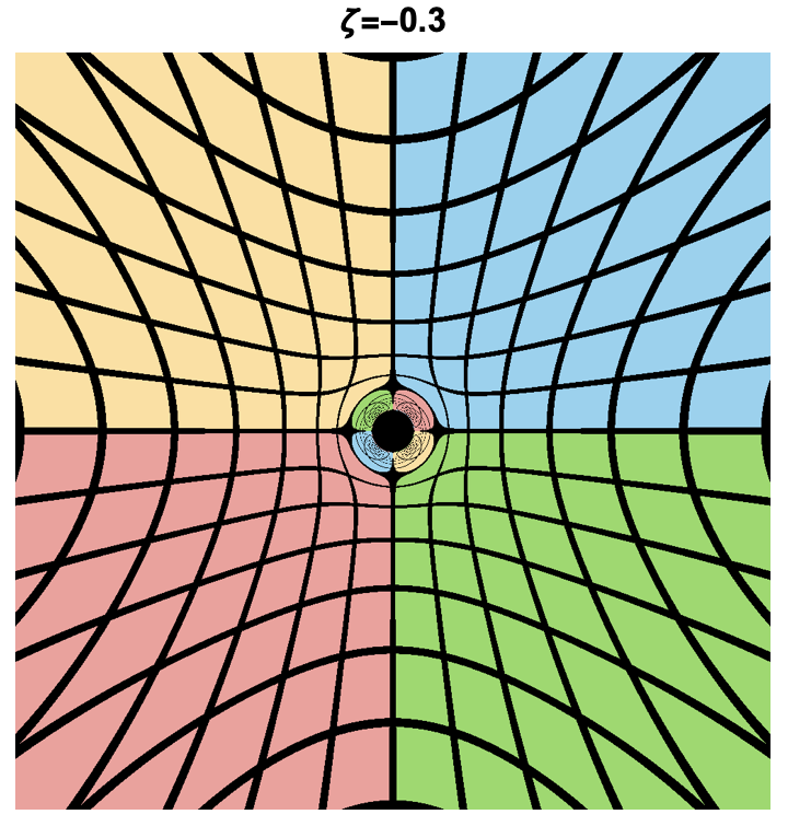
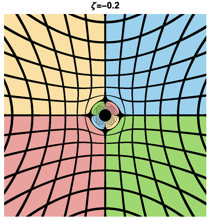
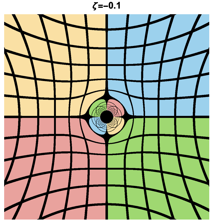
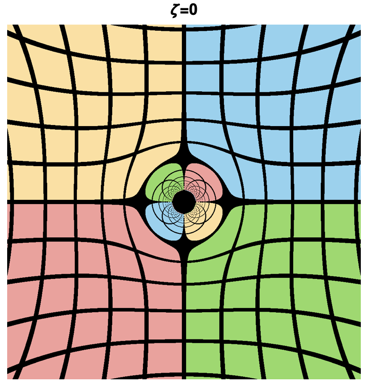
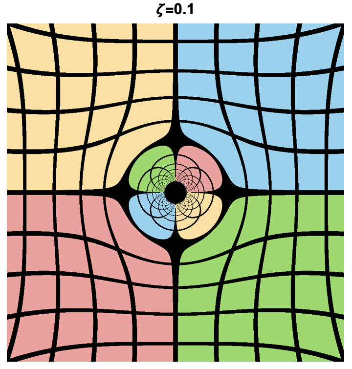
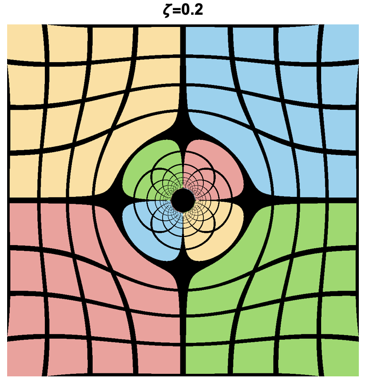
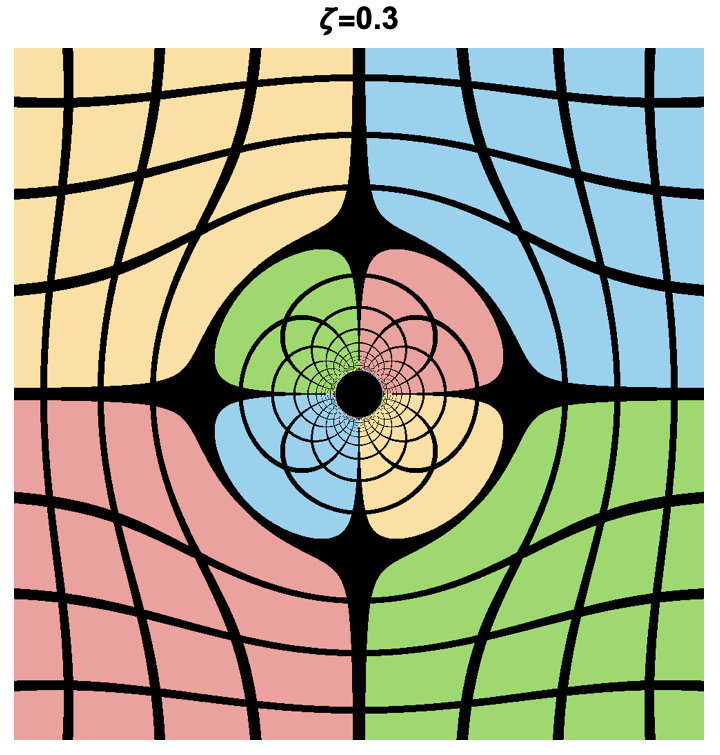
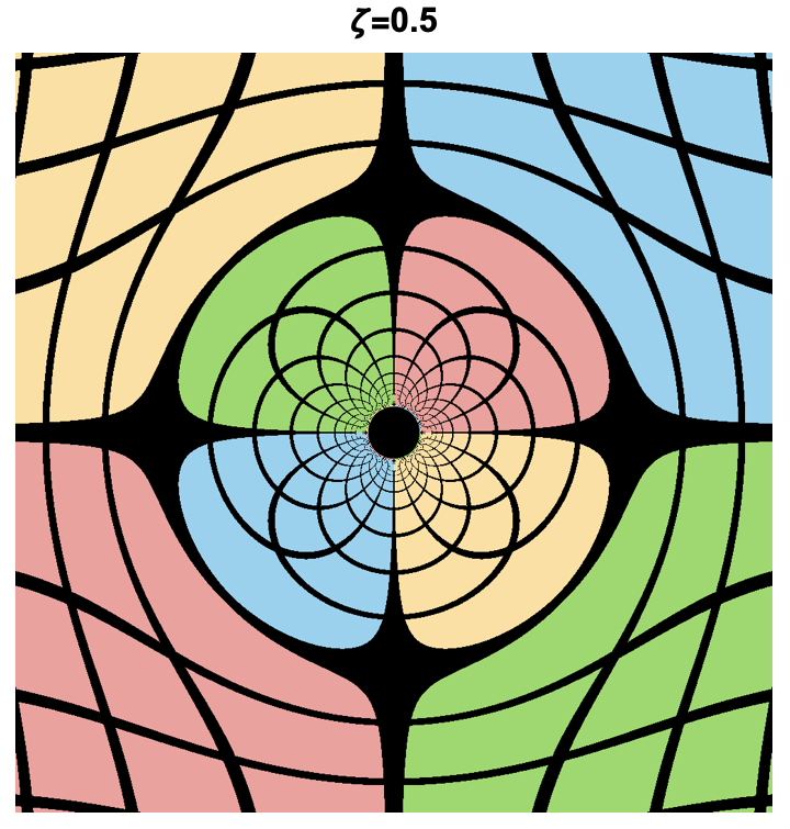
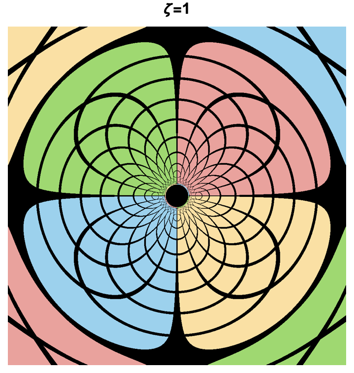
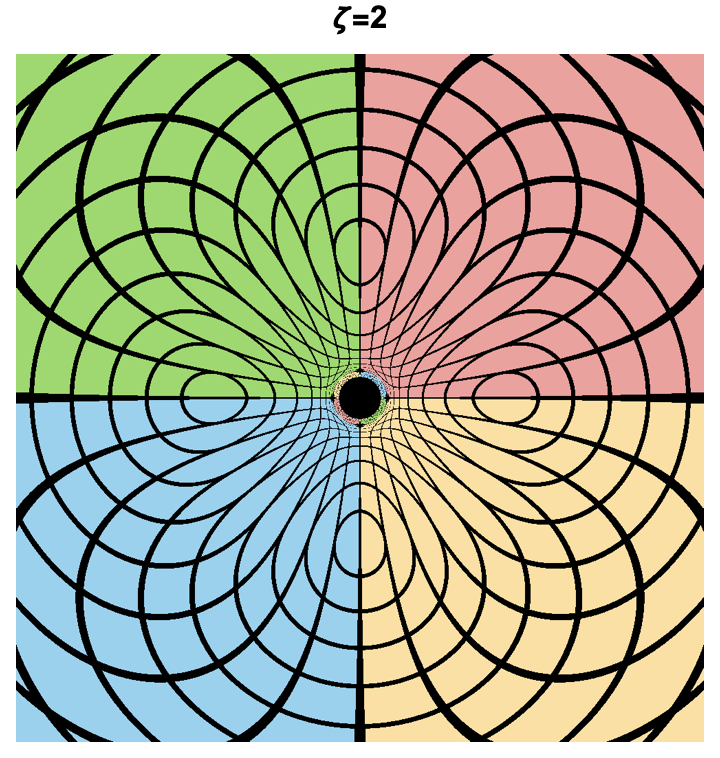
Figure 6: Shadows and lensing rings of the Dunkl black hole by taking the various $\zeta$ values, as seen by an observer at $\theta=\pi/2$.

Fig.6 reveals a notable geometric deformation when the Dunkl parameter $\xi$ deviates significantly from zero, while the shadow radius aligns consistently with the behavior observed in Fig.4.

To furnish the accretion disk images, one should consider a screen with sides of $25M$. This screen, being positioned at $r_{o}=100M$ with asymptotic infinity behaviors for practical purposes, is oriented perpendicular to the observer line of sight toward the black hole. It is split into $500\times 500$ pixels. In order to scrutinize different accretion disk configurations, the observer inclination angles are considered to $\iota=65^{\circ}$ and $85^{\circ}$. Null geodesics are created by working backwards in time from each pixel on the screen to produce the images.

Tab.1 exposes the accretion disk images produced by considering different values the Dunkl parameter $\zeta$ and the observer inclination angle $\iota$.

$\iota$/$\zeta$.	$\zeta=-0.1$	$\zeta=-0.05$	$\zeta=0$	$\zeta=0.2$	$\zeta=0.5$
$85^{\circ}$
$60^{\circ}$

Table 1: Shadows cast by photons tracing null geodesics of the Dunkl black hole by varying $\zeta$.

The morphology of the resulting images of the Dunkl black hole closely looks like those of the Schwarzschild one, although the paramater $\zeta$ significantly influences their appearances.

3.2 Lyapunov exponent

In this part, we deal with the Lyapunov exponent behaviors. It is recalled that the Lyapunov exponents evaluate how the close trajectories in the phase space can be developed. This can quantify the average rate of their divergence or convergence. A positive exponent indicates the divergence behavior, reflecting a high sensitivity to initial conditions. Moreover, the geodesic stability analysis is evaluated throughout the terms of the Lyapunov exponents. Therefore, the unstable circular orbits are intricately connected to the chaotic dynamics around the black holes, making their study valuable for understanding the chaos nature. For instance, Maldacena, Shenker, and Stanford proposed a conjecture suggesting a universal upper limit for Lyapunov exponents $\lambda$, given by

$$\lambda\leq\frac{2\pi T}{\hbar},$$ (27)

where $T$ represents the system temperature [62]. However, as demonstrated in [63], this bound can be exceeded in the case of unstable circular displacements of charged particles in the vicinity of a charged black hole. Furthermore, the unstable circular null geodesics form photon spheres surrounding the event horizon, which are crucial for black hole observational studies.

According to [64], the Lyapunov exponents of the null circular geodesic with unstable motion is expressed in terms of the effective potential given in Eq.(11) as follows

$$\lambda=\sqrt{\frac{r_{\text{c}}^{2}f\left(r_{\text{c}}\right)}{L^{2}}V_{\text{eff}}^{\prime\prime}\left(r_{\text{c}}\right)}.$$ (28)

In Fig.7, we illustrate the logarithmic variation of the Lyapunov exponent in terms of $r$ within various values of the Dunkl parameter $\zeta$.

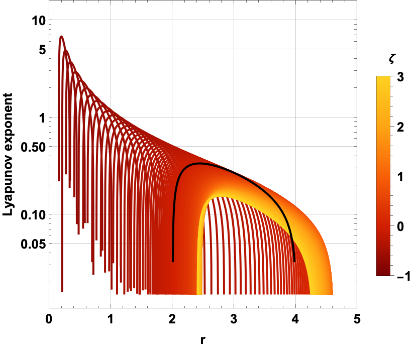
Figure 7: Logarithmic profile of the Lyapunov exponent within different values of the Dunkl parameter $\zeta$, with $M=1$.

The present analysis indicates that the maximum instability tends to rise when there is a reduced contribution from the Dunkl parameter. Conversely, as the variable $r$ increases, the level of instability generally decreases. It is important to highlight that these findings are highly sensitive to the underlying geometric framework. This sensitivity suggests that the present investigation may serve as a significant tool in differentiating between the Schwarzschild black hole solution and the Dunkl black hole.

3.3 Spherically infalling accretion

It has been suggested that an accretion disk arises from a gravitational force of a central object on the surrounding matter such as gas, dust, plasma, including dark matter[65, 66, 20, 19]. As this matter converges towards the center, it gains a kinetic energy producing a promptly rotating disk. The associated disk temperature and the density emit certain radiation forms, such as X-rays, visible lights, or radio waves. These disks play a primordial role in facilitating mass and angular momentum transfer during the gravitating object evaluations. When an accretion disk is aligned with the gravitational lensing effect, it generates an impressive shadow geometry of a black hole. Moreover, it has been suggested that the gravitational lensing is the feature distinguishing the Newtonian and the general-relativistic cases. This can enhance non only the bending of the light but also it underlines the black hole shadow. Its size depends mainly on the black hole intrinsic parameters. Its contour, however, remains dynamic due to the instability of the light rays from the photon sphere. To distant observers, the shadow appears as a dark. This is a two-dimensional disk, being beautifully set against its bright with uniform surroundings.

In this section, we are interested in spherically free-falling accretion around the Dunkl black hole, originating from an infinite distance. The present investigation is based on the approach proposed in [65, 66, 20]. Inspired by such a work, we provide a realistic representation of the accretion disk shadow.

Roughly, we would like to inspect the impact of the Dunkl parameter $\zeta$ on the spacetime structure and the observational characteristics. Sending the observer to the infinity, the observation specific intensity (measured usually in $\rm ergs^{-1}cm^{-2}str^{-1}Hz^{-1}$) can be determined using the techniques developed in [65, 20]. Indeed, it is expressed as follows

$${I}_{obs}(\nu_{obs},b)=\int_{\Gamma}g^{3}j(\nu_{e})d\ell_{{prop}},$$ (29)

where $g$ represent the redshift factor. It denoted that $\nu_{e}$ and $\nu_{obs}$ are the photon frequency and the observed photon frequency, respectively, $b$ stands for the impact parameter. Considering the emitter in the rest frame, $j(\nu_{e})\propto\frac{\delta\left(\nu_{e}-\nu_{f}\right)}{r^{2}}$ is the emissivity per unit volume, proportional to the $1/r^{2}$ radial profile [20] via the delta function $\delta$. $\nu_{f}$ is the light radiation frequency being assumed to be monochromatic. $d\ell_{{prop}}$ denotes the infinitesimal proper length. Taking a black hole geometry, the redshift factor can be written as

$$g=\frac{\hat{\mathcal{K}}_{\rho}u_{0}^{\rho}}{\hat{\mathcal{K}}_{\sigma}u_{e}^{\sigma}},\quad\hat{\mathcal{K}}^{\mu}=\dot{x}_{\mu},$$ (30)

where $\hat{\mathcal{K}}^{\mu}$ indicates the four-velocity of the photon. $u_{0}^{\mu}$ is the four-velocity of the static observer being identified with $=(1,0,0,0)$. However, the quantity $u_{e}^{\mu}$ indicates the four-velocity of the infalling accretion involving the form

$$u_{e}^{t}={f(r)}^{-1},\quad u_{e}^{r}=-\sqrt{{1-f(r)}},\quad u_{e}^{\theta}=u_{e}^{\varphi}=0.$$ (31)

Taking a null geodesic, we could extract the photon four-velocity. Indeed, it is given by

$$\hat{\mathcal{K}}_{t}=\frac{1}{b},\quad\frac{\hat{\mathcal{K}}_{r}}{\hat{\mathcal{K}}_{t}}=\pm\frac{1}{f(r)}\sqrt{1-f(r)\frac{b^{2}}{r^{2}}}.$$ (32)

In this way, the sign $\pm$ characterize the situation where the photon trajectory is either towards or away from the black hole. Thus, the redshift factor of the infalling accretion enhances

$$g=\left(u_{e}^{t}+\left(\frac{\hat{\mathcal{K}}_{r}}{\hat{\mathcal{K}}_{e}}\right)u_{e}^{r}\right)^{-1}.$$ (33)

On the other hand, the proper distance should take the form

$$d\ell_{prop}=\hat{\mathcal{K}}_{\mu}u_{e}^{\mu}d\lambda=\frac{\hat{\mathcal{K}}_{t}}{g|\hat{\mathcal{K}}_{r}|}dr.$$ (34)

Integrating Eq.(29) over all possible frequencies, we could obtain the observation intensity for the infalling spherical accretion. The computation leads to

$$I_{{obs}}\propto\int_{\Gamma}\frac{\mathcal{G}_{i}^{3}\hat{\mathcal{K}}_{t}dr}{r^{2}|\hat{\mathcal{K}}_{r}|}.$$ (35)

Using the above equations, we explore the shadow and brightness of the power Dunkel black hole, surrounded by the infalling spherical accretion. In Fig.8, we depict the luminosity distribution by considering different values of the parameter $\zeta$.

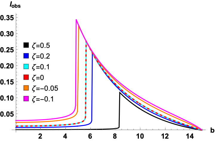
Figure 8: , Observed specific intensity at spatial infinity with $M=1$ in terms of the impact parameter, for different power parameter parameter values $\zeta$

From this figure, we can observe that the specific intensity $I_{obs}$ augments stylishly with the impact parameter $b$ and then it reaches a peak value in the critical case $b\sim b_{ph}$. This universal behavior has appeared for different values of the Dunkl parameter $\zeta$. For $b>b_{c}$, the specific intensity $I_{obs}$ involves a trending down. In the limit where $b$ goes to infinity, the observation intensity vanishes, namely $I_{obs}\sim 0$.

Fig.9 presents a two-dimensional picture of the observed shadows of the Dunkl black hole in terms of $\xi$.

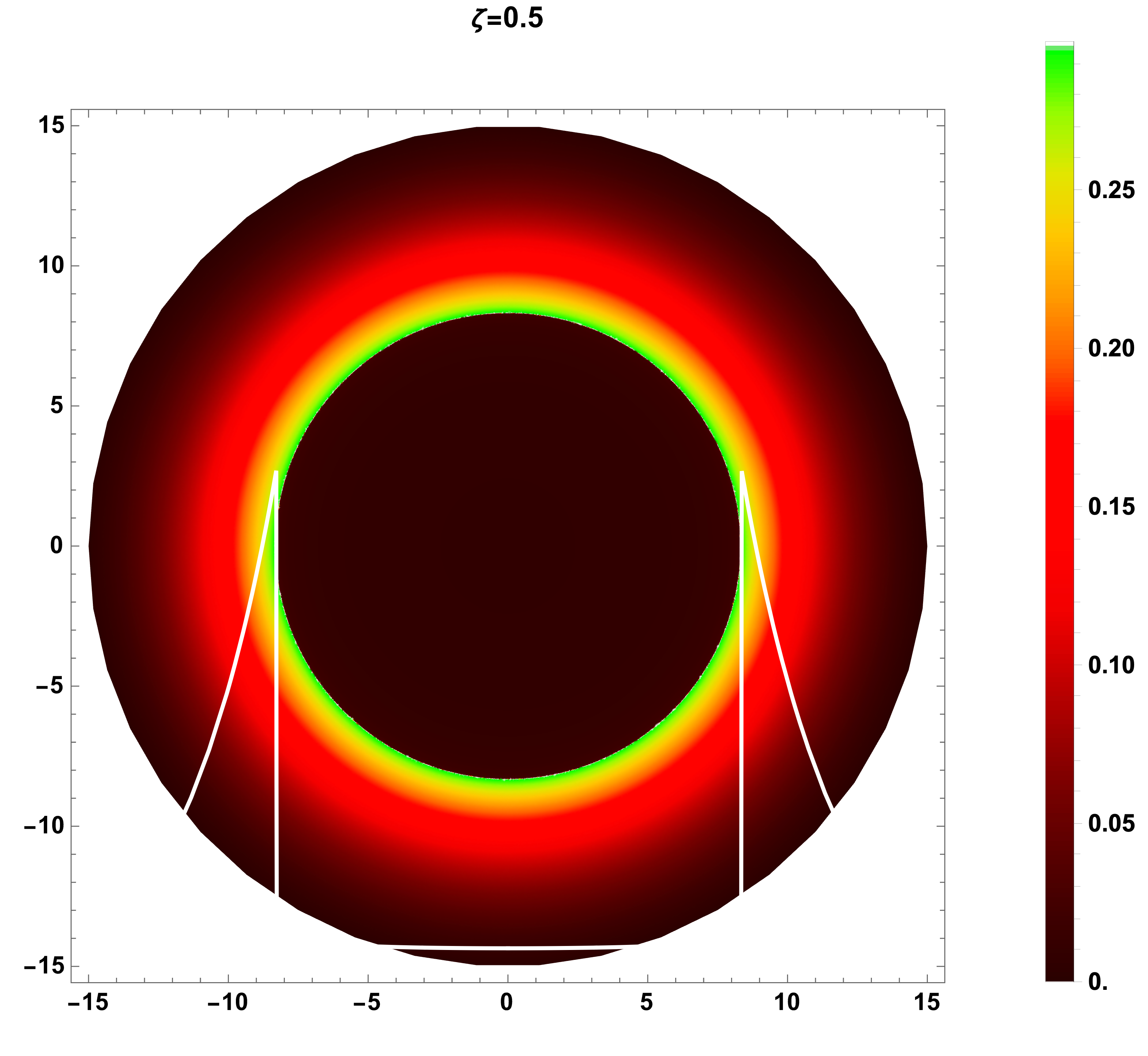
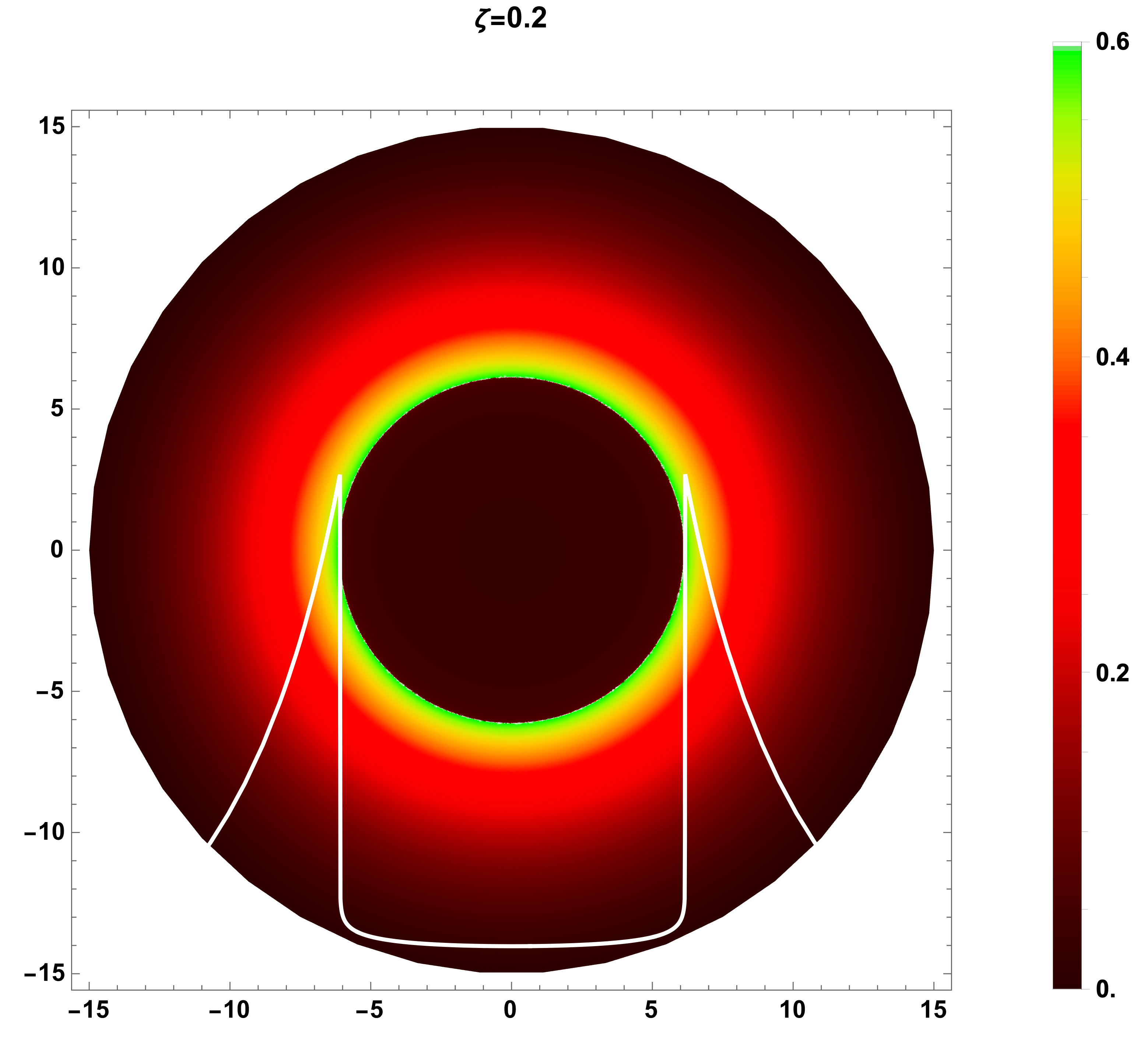
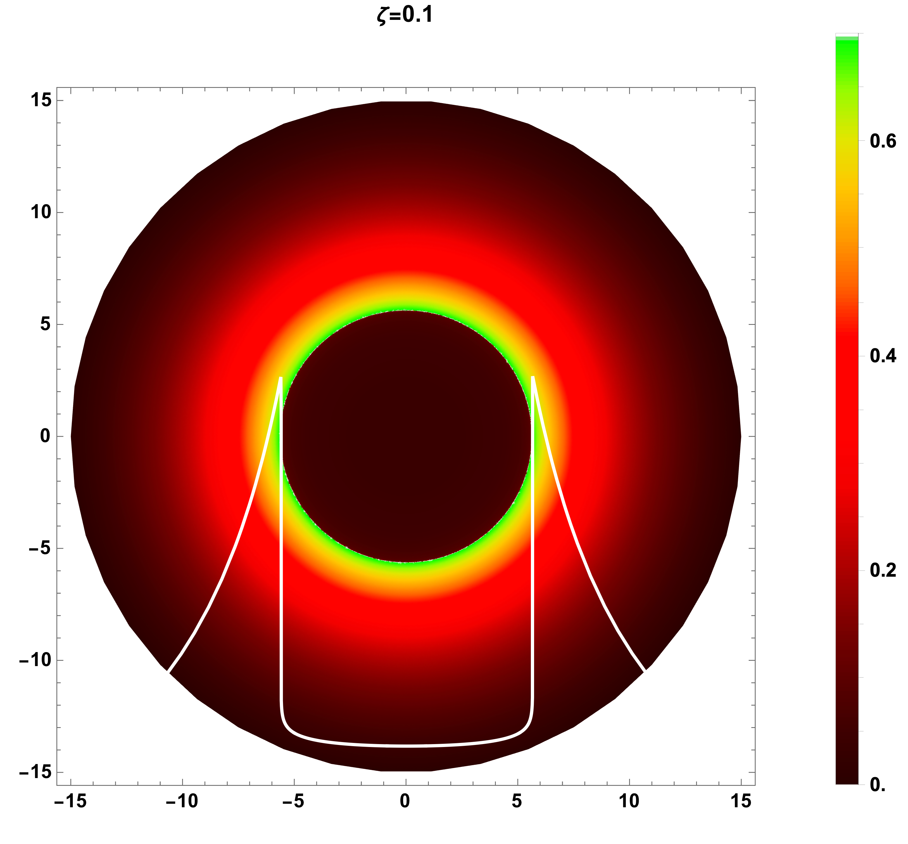
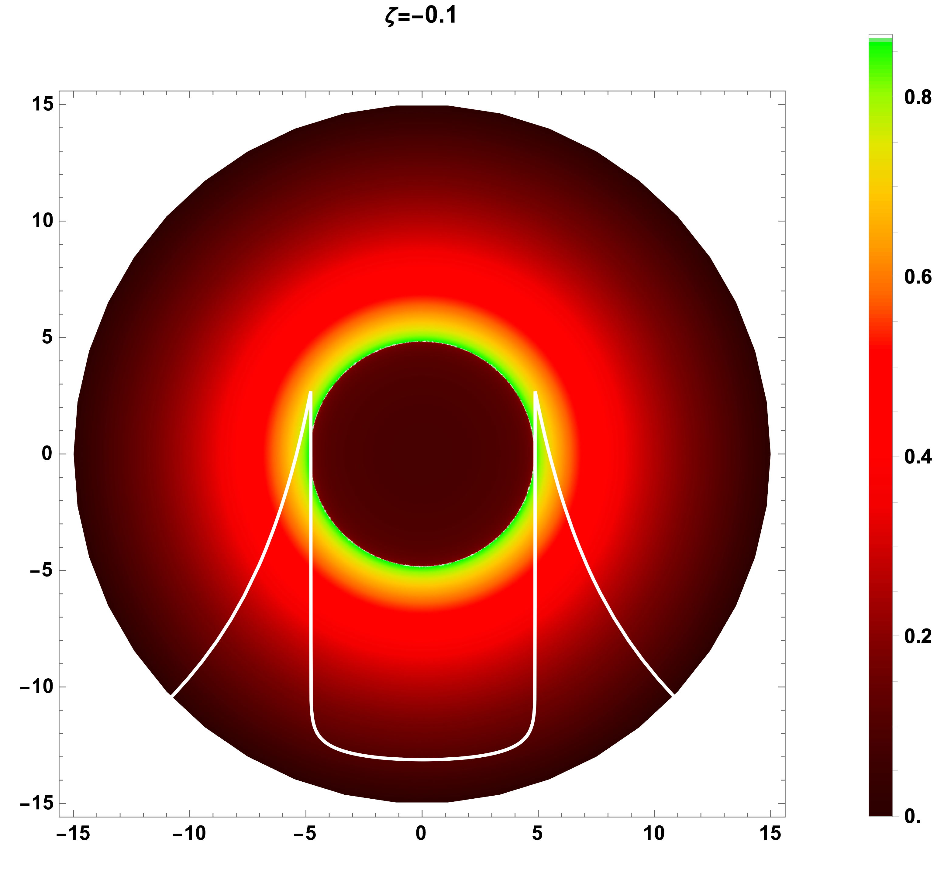
Figure 9: Black hole shadows with spherical accretion by varying Dunkel parameter $\zeta$.

It has been observed that a bright ring with a higher luminosity is situated in close proximity to the photon sphere. Moreover, the inner region of the photon sphere is not entirely devoid of light. It has been remarked a small luminosity near to the photon sphere. This has been explained by a radiation tiny fraction escaped from the black hole. As anticipated, increasing the parameter $\zeta$ leads to an expansion in the black hole shadow size, while it simultaneously reduces the maximum luminosity of the shadow image. This behavior is consistent with the trends observed in Fig.8.

3.4 Light deflection angle in vacuum and medium backgrounds

Now, we move to discuss the behaviors of the light deflection angle by the Dunkl black hole by focusing on the effect of the involved parameter. There are several methods available to compute this optical quantity. Notably, Gibbons and Werner have utilized the Gauss-Bonnet theorem [44, 67], which connects the differential geometry of a surface to its topology. By applying the optical geometry, one can compute the deflection angle of light rays passing near various spherically symmetric black hole geometries. Here, we adopt these techniques to derive the expression for the deflection angle in the weak-field limit induced by the Dunkl black hole.

We begin by calculating the optical metric on the equatorial plane, being given by $\theta=\pi/2$, using the line element (1). Precisely, one finds

$$dt^{2}=\frac{dr^{2}}{f(r)^{2}}+\frac{r^{2}}{f(r)}d\phi^{2}\,.$$ (36)

The Gaussian optical curvature $\bar{K}=\frac{\bar{R}}{2}$, where $\bar{R}$ is the Ricci scalar of the optical metric (36), takes the following form

$$\bar{K} = M\left(-\frac{2}{r^{3}}+\frac{4\zeta\log(r)}{3r^{3}}-\frac{4\zeta^{2}\log(r)(3\log(r)+2)}{27r^{3}}\right)$$ (37)

$$+ M^{2}\left(\frac{3}{r^{4}}+\frac{2\zeta(4-6\log(r))}{3r^{4}}+\frac{\zeta^{2}(72(\log(r)-1)\log(r)-4)}{27r^{4}}\right)+\mathcal{O}(M^{3},\zeta^{3}).$$

To calculate the deflection angle, it is essential to consider a non-singular manifold $\mathcal{D}_{\tilde{R}}$ with a geometric scale $\tilde{R}$ to apply the Gauss-Bonnet theorem. According to [44, 67], one has

$$\int\int_{\mathcal{D}_{\tilde{R}}}\bar{K}dS+\oint_{\partial\mathcal{D}_{\tilde{R}}}kdt+\sum_{i}\varphi_{i}=2\pi\varrho(\mathcal{D}_{\tilde{R}})\,,$$ (38)

where one used $dS=\sqrt{\bar{g}}drd\phi$ and $dt$ represent the surface and line elements of the optical metric in Eq.(36), respectively. Here, $\bar{g}$ is the determinant of the optical metric. $k$ is the geodesic curvature of $\mathcal{D}_{\tilde{R}}$. $\varphi_{i}$ indicates the exterior angle at the $i$-th vertex. Additionally, $\varrho(\mathcal{D}_{\tilde{R}})$ represents the Euler characteristic of $\mathcal{D}_{\tilde{R}}$, which can be set to $\varrho(\mathcal{D}_{\tilde{R}})=1.$ For a smooth curve $y$ with a tangent vector $\dot{y}$ and an acceleration vector $\ddot{y}$, we can define the geodesic curvature $k$ of $y$ via the speed constraint $\tilde{g}\left(\dot{y},\dot{y}\right)=1$. Indeed, it is given by

$$k=\tilde{g}\left(\nabla_{\dot{y}\dot{y},\ddot{y}}\right),$$ (39)

which measures the deviations of $y$ from a geodesic. In the limit where $\tilde{R}\rightarrow\infty$, the two jump angles $\varphi_{s}$ (at the source) and $\varphi_{o}$ (at the observer) approach $\pi/2$, leading to $\varphi_{s}+\varphi_{o}\rightarrow\pi$. For the curve $C_{\tilde{R}}:=r(\phi)$, the geodesic curvature is $k(C_{\tilde{R}})=|\nabla_{\dot{C}{\tilde{R}}}\dot{C}{\tilde{R}}|,,,\mathrel{\stackrel{{\scriptstyle\makebox[0.0pt]{\mbox{\tiny$\tilde{R}\rightarrow\infty$}}}}{{\rightarrow}}},,,1/\tilde{R}$, and we obtain $\lim_{\tilde{R}\rightarrow\infty}dt=\tilde{R}d\phi$. Thus, one has $k(C_{\tilde{R}})dt=d\phi$. In fact, the Gauss-Bonnet theorem simplifies to the form

$$\int\int_{\mathcal{D}_{\tilde{R}}}\bar{K}dS+\oint_{C_{\tilde{R}}}kdt\,\,\,\mathrel{\stackrel{{\scriptstyle\makebox[0.0pt]{\mbox{\tiny$\tilde{R}\rightarrow\infty$}}}}{{=}}}\,\,\,\int\int_{\mathcal{D}_{\infty}}\bar{K}dS+\int_{0}^{\pi+\Theta}d\phi=\pi\,.$$ (40)

Exploiting techniques for calculating the deflection angle (see Refs [44, 67] and references therein), one gets

$$\Theta=\pi-\int_{0}^{\pi+\Theta}d\phi=-\int_{0}^{\pi}\int_{\frac{\xi}{\sin\phi}}^{\infty}\bar{K}dS\,.$$ (41)

Combining the above equations, the Gaussian optical curvature for the Dunkel dark compact object is found to be

$$\bar{K} \approx M\left(-\frac{2}{r^{2}}+\zeta\left(\frac{4\log(r)}{3r^{2}}-\frac{3}{r^{2}}\right)+\zeta^{2}\left(-\frac{3}{4r^{2}}-\frac{4\log^{2}(r)}{9r^{2}}+\frac{46\log(r)}{27r^{2}}\right)\right)$$

$$+ M^{2}\left(-\frac{3}{r^{3}}+\zeta\left(\frac{4\log(r)}{r^{3}}-\frac{47}{6r^{3}}\right)+\zeta^{2}\left(-\frac{1355}{216r^{3}}-\frac{8\log^{2}(r)}{3r^{3}}+\frac{86\log(r)}{9r^{3}}\right)\right)+\mathcal{O}(M^{3},\zeta^{3}).$$

Moreover, the optical metric (36) for the Dunkl dark compact object, in accordance with the metric coefficients (1), can be approximated as

$$dS=\sqrt{\bar{g}}\,drd\phi=\frac{r}{h(r)\sqrt{f(r)}}dtd\phi\approx rdrd\phi\,.$$ (43)

In this way, the deflection angle for the Dunkl black hole can be expressed as follows

$$\begin{split}\Theta&=-\int_{0}^{\pi}\int_{\frac{\xi}{\sin\phi}}^{\infty}\bar{K}dS.\end{split}$$ (44)

After computations, this quantity is found to be

$$\begin{split}\Theta&\approx M\Big{\{}\frac{4}{b}+\frac{\zeta}{3b}\Big{[}2+\log(256)-8\log(b))\Big{]}+\frac{\zeta^{2}}{54b}\Big{[}48\log^{2}(b)+(8-96\log(2))\log(b)\\ &-4\pi^{2}+1+8\log(2)(\log(8)-1)\Big{]}\Big{\}}+M^{2}\Big{\{}\frac{3\pi}{4b^{2}}+\frac{\zeta\pi}{24b^{2}}\Big{[}47-12\log(4)-24\log(b)\Big{]}\\ &+\frac{\zeta^{2}\pi}{864b^{2}}\Big{[}48\log(b)(12\log(4b)-43)+48\pi^{2}+1067+24\log(4)(6\log(4)-43)\Big{]}\Big{\}}+\mathcal{O}(M^{3},\zeta^{3})\end{split}$$ (45)

Having expressed the deflection angle for such a black hole in the vacuum medium, we move to illustrate graphically the effect of the Dunkl parameter on this quantity. Indeed, we depict in Fig.10 the light deflection angle $\Theta$ in terms of the impact parameter $b$.

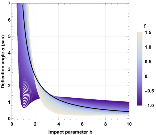
Figure 10: Observed specific intensity at spatial infinity with $M=1$ in terms of the impact parameter by taking certain parameter values $\zeta$.

From Fig.10, we can observe that the deflection angle behavior shows a minimum for $\zeta\leq-0.8$. Then, it increases and after that it decreases gradually and goes to positive infinity. As $\zeta$ grows the minimum point, it disappears and only the decreasing behaviors persists. In reality, the astrophysical objects are typically enveloped by an interstellar medium, often modeled as plasma in the event horizon vicinity. As photons traverse this plasma, their interactions with the medium modify their trajectories. This interaction, in turn, influences the apparent size of the central shadow as seen by a distant observer.

To incorporate plasma effects, we assume that the photon travels from a vacuum into a hot, ionized gas medium, where $v$ is the light speed in the plasma. Indeed, the refractive index, $n(r)$, can then be expressed as follows

$$n_{\text{Plasma}}(r)\equiv\frac{v}{c}=\frac{1}{dr/dt},\quad\quad\{\because c=1\}.$$ (46)

Following [68, 69], the refractive index $n(r)$ for the associated black hole reads as

$$n_{\text{Plasma}}(r)=\sqrt{1-\frac{\omega_{e}^{2}}{\omega_{\infty}^{2}}f(r)},$$ (47)

where $\omega_{e}$ denotes the electron plasma frequency. $\omega_{\infty}$ represents the photon frequency as observed at infinity. Consequently, the line element in Eq.(1) transforms into the following form

$$dt^{2}=g_{ij}^{opt}dx^{i}dx^{j}=n_{\text{Plasma}}^{2}(r)\left[\frac{dr^{2}}{f(r)^{2}}+\frac{r^{2}d\phi}{f(r)}\right].$$ (48)

The deflection angle, originally derived under vacuum conditions, could take a new form influenced by the plasma properties. Indeed, it can be expressed as follows

$$\Theta_{\text{Plasma}} \approx \left\{\left(\frac{4}{b}+\frac{2\omega_{e}}{b\omega_{\infty}}+\frac{2\omega_{e}^{2}}{b\omega_{\infty}^{2}}\right)+\left(\frac{2(-4\log(b)+1+\log(16))}{3b}\right.\right.$$ (49)

$$+ \left.\left.\frac{2(-4\log(b)+1+\log(16))}{3b}+\frac{\omega_{e}^{2}(-4\log(b)-9+\log(16))}{3b\omega_{\infty}^{2}}\right)\zeta\right\}M$$

$$+ \left\{\left(\frac{3\pi}{4b^{2}}-\frac{\pi\omega_{e}}{2\left(b^{2}\omega_{\infty}\right)}-\frac{3\pi\omega_{e}^{2}}{2b^{2}\omega_{\infty}^{2}}\right)\right.+\left(\frac{-24\pi\log(b)+47\pi-12\pi\log(4)}{24b^{2}}\right.$$

$$+ \left.\left.\frac{\omega_{e}(8\pi\log(b)-11\pi+\pi\log(256))}{12b^{2}\omega_{\infty}}+\frac{\omega_{e}^{2}(8\pi\log(b)-5\pi+\pi\log(256))}{4b^{2}\omega_{\infty}^{2}}\right.\right.$$

$$+ \left.\left.\frac{\omega_{e}^{2}(8\pi\log(b)-5\pi+\pi\log(256))}{4b^{2}\omega_{\infty}^{2}}\right)\zeta\right\}M^{2}+\mathcal{O}(M^{3},\zeta^{2},\omega_{e}^{3}).$$

The presence of a medium introduces significant dispersion effects on the light rays instead of propagation in a vacuum. One possibility of such a medium, consistently found in astrophysical contexts, is dark matter, which often forms vast halos around black holes, as observed by EHT [70, 71, 72]. It has been remarked that the Dark matter has the ability to enshroud entire galaxies and permeate both interstellar and intergalactic spaces being a central point of certain scientific investigations[73, 74, 75]. Combining the dark matter with black holes provides essential insights into gravitational lensing phenomena. To assess the impact of dark matter on the deflection angle of light, we derive the refractive index based on scatterers in the medium, as detailed in references[39, 76, 42]. Indeed, we have

$$n_{\text{DM}}=1+\mathcal{B}u+vw^{2},$$ (50)

where $w$ denotes the light frequency. The quantity $\mathcal{B}$ is identified with $=\rho_{0}/4mw^{2}$ where $\rho_{0}$ is the mass density of the dark matter particles, and $m$ is their mass. The parameter $u=-2\epsilon^{2}e^{2}$ is defined. It is denoted that $\epsilon$ is the charge of the scattered matter in units of $e$. $v$ represents a non-negative value. Higher order $\mathcal{O}(w^{2})$ and account for the polarizability of the dark matter particle could define the refractive index for an optically inactive medium. Specifically, the $w^{-2}$ term is associated with a charged dark matter candidate, while the $w^{2}$ term corresponds to a neutral candidate. It is worth noting that, a linear term in $w$ may appear once one has the parity and the charge parity asymmetries.

Recalling the optical metric Eq.(48) with the optical index Eq.(50), the deflection angle associated with the Dunkel black hole enveloped by dark matter can be given by

$$\Theta_{\text{DM}}=\frac{\Theta}{\left(1+\mathcal{B}u+vw^{2}\right)^{2}}.$$ (51)

The analysis reveals that the deflection angle rises by increasing values of the parameter $w$ within the weak field regime. This trend suggests that heightened dark matter activity intensifies lensing profile distortions. While the dynamics of dark matter near black holes are not as well understood as its distribution in outer-galactic regions, its essential role in enhancing both the distortions and the resulting deflection angle remains a consistent and significant factor.

4 Constraints from EHT observations of $\textrm{M87}^{\star}$ and $\textrm{Sgr\leavevmode\nobreak\ A}^{\star}$ black holes

In this section, we aim to compare the shadow results obtained from our analysis with the observations of the supermassive black holes captured by EHT. This comparison constrains the Dunkl parameter $\zeta$ by utilizing the observational data of $\textrm{M87}^{\star}$ and $\textrm{Sgr\leavevmode\nobreak\ A}^{\star}$ provided by the EHT international collaboration.

Specifically, we focus on the key observables related to the black hole shadows: the angular diameter $\mathcal{D}$ and the deviation from the Schwarzschild geometry ${\bm{\delta}}$. By matching our theoretical predictions with the observed data for $\textrm{M87}^{\star}$ and $\textrm{Sgr\leavevmode\nobreak\ A}^{\star}$, we wouyld like to establish tighter constraints on the Dunkl parameter. According to [77], the angular diameter $\mathcal{D}$ is a crucial observable defined as

$$\mathcal{D}=\frac{Gm}{c^{2}}\left(\frac{\Delta Y}{d}\right),$$ (52)

where $d$ denotes the distance from Earth to $\textrm{M87}^{\star}$ or $\textrm{Sgr\leavevmode\nobreak\ A}^{\star}$. Moreover, $\Delta Y$ represents the maximum length of the shadow along the direction $Y$ in the $(X,Y)$ plane, being orthogonal to the $X$ axis. The EHT collaboration provides the deviation parameter ${\bm{\delta}}$ to quantify the difference between the infrared shadow radius. For the Schwarzschild black hole [78], it takes the form

$${\bm{\delta}}=\frac{r_{\text{s}}}{r_{\text{Sch}}}-1.$$ (53)

According to EHT collaboration [1, 27, 28], the observed parameters of the supermassive black hole $\textrm{M87}^{\star}$ at the center of the $\textrm{M}87$ galaxy include an angular diameter of $\mathcal{D}=42\pm 3\mu$as and a fractional deviation ${\bm{\delta}}$ from the predicted Schwarzschild black hole shadow diameter reported by the EHT [31]. The latter remains consistent regardless of the telescope, image processing techniques, or used simulations. Based on the black hole image of $\textrm{M87}^{\star}$ [48], detailed values for ${\bm{\delta}}$ are provided in Tab.2

	$\textrm{M}87^{\star}$ estimates
	Deviation ${\bm{\delta}}$	$\text{1-}\sigma$ bounds	$\text{2-}\sigma$ bounds
EHT	$-0.01^{+0.17}_{-0.17}$	$4.26\leq\frac{r_{\text{sh}}}{M}\leq 6.03$	$3.38\leq\frac{r_{\text{sh}}}{M}\leq 6.91$

	Sgr $A^{*}$ estimates
		Deviation $\delta$	1-$\sigma$ bounds	2-$\sigma$ bounds
eht-img	VLTI	$-0.08^{+0.09}_{-0.09}$	$4.31\leq\frac{r_{\text{sh}}}{M}\leq 5.25$	$3.85\leq\frac{r_{\text{sh}}}{M}\leq 5.72$
	Keck	$-0.04^{+0.09}_{-0.10}$	$4.47\leq\frac{r_{\text{sh}}}{M}\leq 5.46$	$3.95\leq\frac{r_{\text{sh}}}{M}\leq 5.92$
mG-ring	VLTI	$-0.17^{+0.11}_{-0.10}$	$3.79\leq\frac{r_{\text{sh}}}{M}\leq 4.88$	$3.27\leq\frac{r_{\text{sh}}}{M}\leq 5.46$
	Keck	$-0.13^{+0.11}_{-0.11}$	$3.95\leq\frac{r_{\text{sh}}}{M}\leq 5.09$	$3.38\leq\frac{r_{\text{sh}}}{M}\leq 5.66$

Table 2: Top: $\textrm{M}87^{\star}$ bounds on the deviation parameter $\bm{\delta}$ and dimensionless shadow radius $r_{\text{sh}}/M$. Bottom: Sagittarius A* bounds on the deviation parameter $\delta$ and shadow radius[79].

For $\textrm{M87}^{\star}$, the central value of ${\bm{\delta}}$ tends toward zero, but uncertainties in mass and distance measurements contribute to larger error margins. Utilizing the value of ${\bm{\delta}}$ from Eq. (53) and Tab.2, one can impose constraints on the black hole parameters by considering the dimensionless quantity $r_{\text{s}}/M$. Additionally, an inclination angle of $17^{\circ}$ is predicted, corresponding to the angle formed between the jet axis and the observer line of sight, assuming the rotation axis aligns with the jet. The EHT collaboration estimates the distance to $\textrm{M87}^{\star}$ to be $d=16.8\pm 0.8$ Mpc, with the mass calculated as $m=(6.5\pm 0.7)\times 10^{9}M_{\odot}$. The angular diameter of the black hole shadow is estimated at $42\pm 3\mu$as, with a $10\%$ correction applied to account for the offset between the image and the shadow, yielding a minimum shadow diameter of $37.8\pm 2.7\mu$as.

For $\textrm{Sgr\leavevmode\nobreak\ A}^{\star}$, the observed emission ring diameter is reported as $51.8\pm 2.3\mu$as by the EHT collaboration [2], while the estimated shadow diameter is $48.7\pm 7\mu$as. Multiple teams have measured the mass and distance to $\textrm{Sgr\leavevmode\nobreak\ A}^{\star}$. Data from the Keck Observatory show a distance of $d=(7959\pm 59\pm 32)$ pc and a mass of $m=(3.975\pm 0.058\pm 0.026)\times 10^{6}M_{\odot}$, where the redshift parameter is treated as free. Assuming a redshift of unity gives a distance of $d=(7935\pm 50)$ pc and a mass of $m=(3.951\pm 0.047)\times 10^{6}M_{\odot}$ [80]. Similarly, the GRAVITY collaboration from the Very Large Telescope Interferometer (VLTI) reports a mass of $m=(4.261\pm 0.012)\times 10^{6}M_{\odot}$ and a distance of $d=(8246.7\pm 9.3)$ pc [81, 82]. When accounting for optical aberrations, these measurements suggest a mass of $m=(4.297\pm 0.012\pm 0.040)\times 10^{6}M_{\odot}$ and a distance of $d=8277\pm 9\pm 33$ pc. Furthermore, numerical models suggest that the inclination angle $i$ of $\textrm{Sgr\leavevmode\nobreak\ A}^{\star}$ is greater than $50^{\circ}$. Our analysis uses an inclination value of $i\simeq 134^{\circ}$ (or equivalently $46^{\circ}$) [83]. Using the eht-img algorithm [31], the fractional deviation $\bm{\delta}$ and the dimensionless shadow radius $r_{\text{s}}/M$ have been computed. They are presented at the bottom of Tab.2.

Fig.11 illustrates the shadow radius $r_{\text{sh}}/M$ of the Dunkl black hole compared with the EHT shadow size of M87^∗ within 1-$\sigma$ and 2-$\sigma$ bonds by varying the Dunkl parameter.

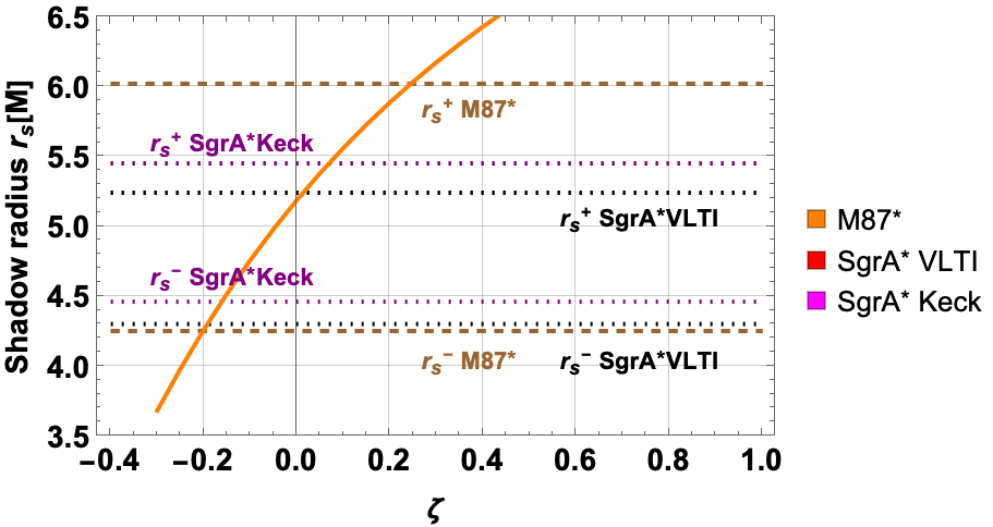
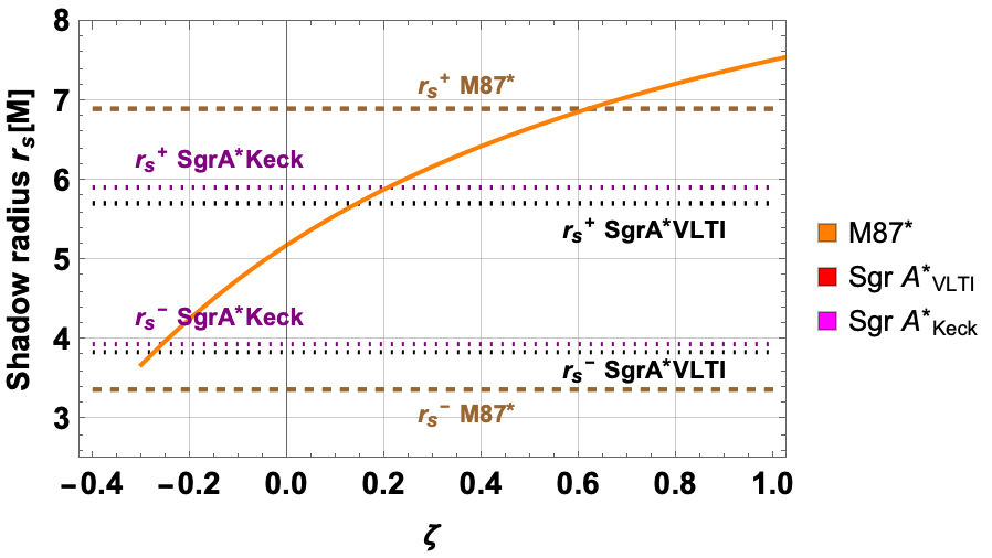
Figure 11: Shadow radius for Dunkl black hole with M87^∗ and SgrA^∗ observed data, Left: within the 1-$\sigma$ and Right: the 2-$\sigma$ bounds.

It is evident that the curves overlap due to the rescaling of mass, with distinctions arising from the specific experimental bounds associated with each black hole. In this sense, Fig.11 involves acceptable and excluded regions, being compatible and incompatible with the EHT observations. It gives information on the ranges of $\zeta$ in accordance with EHT collaborations. Within the M87^∗ data, in the 1-$\sigma$ confidence level, the range $-0.2043\leq\zeta\leq 0.2432$ generates consistent results. This range has been enlarged in the 2-$\sigma$ confidence level. The range $\zeta>0.6191$, however, provides discordant results with respect to EHT. While for SgrA^∗, we have found the $-0.194\leq\zeta\leq 0.0122$, $-0.2756\leq\zeta\leq 0.1444$ within the Keck data and $-0.163\leq\zeta\leq 0.0679$, $-0.2574\leq\zeta\leq 0.270$ for the VLTI measurements, respectively. Going further, we would like to constraint the Dunkl parameter using the angular diameter $\mathcal{D}$ and the fractional deviation ${\bm{\delta}}$ engineered by EHT collaboration from Keck and VLTI observations as depicted in Fig.12.

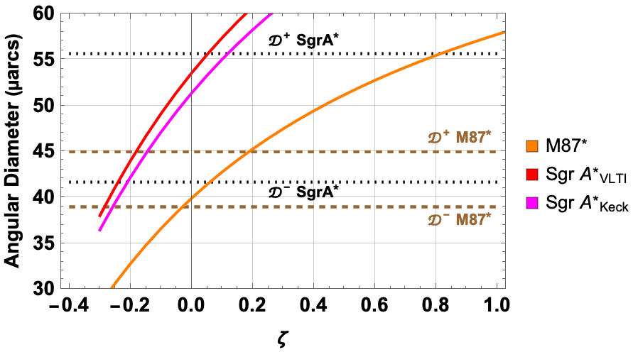
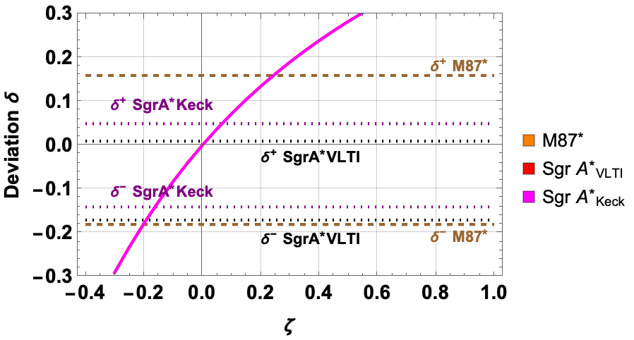
Figure 12: Angular diameter $\mathcal{D}$ and fractional deviation $\bm{\delta}$ in terms of the Dunkl parameter associated with M87^∗ and SgrA^∗ black hole observed data.

In addition to the previous requirements on the Dunkl parameter $\zeta$ elaborated from the shadow radius $r_{s}/M$, the constraint derived from the angular diameter $\mathcal{D}$ and the fraction deviation $\bm{\delta}$ illustrated in Fig.12 are summarized in Tab.3.

		Dunkl parameter $\zeta$
		$\mathcal{D}$	$\bm{\delta}$	$r_{s}/M$
				1-$\sigma$	2-$\sigma$
M87∗		[-0.0316 , -0.0316]	[-0.2044 , 0,2448]	[-0.2043 , 0.2432]	[— , 0.6191]
SgrA∗	Keck	[-0.2418 , 0,0524]	[-0.1924 , 0.0122]	[-0.194 , 0.0122]	[-0.2756 , 0.1444]
	VLTI	[-0.2112 , 0.1174]	[-0.1643 , 0.0663]	[-0.163 , 0.0679]	[-0.2574 , 0.270]

Table 3: Estimations of the Dunkel parameter $\zeta$ within the observables $\mathcal{D}$, $\bm{\delta}$ and $r_{s}/M$ for SgrA^∗ and M87^∗ black holes

5 Conclusion

In this paper, we have reconsidered the study of the Dunkl black hole by focusing on the optical aspect. It has shown that such a black hole has been obtained by combining the Dunkl operator formalism and the Einstein gravity equations. The computations have provided a black hole solution involving a relevant parameter refereed to as $\xi$. After a concise geometric discussion on such a solution, we have investigated two optical concepts: the shadow and the deflection angle. Such notions have been studied by varying the Dunkl parameter. As expected, we have found shadow circular geometries since we have considered non-rotating solutions. The size of the obtained shadows depends on the Dunkl parameter. We have revealed that the circular shadow size augments with the parameter $\xi$. Considering small values of the impact parameter, we have observed that the deflection angle of light rays decreases with such a parameter. However, the deflection angle of the light rays becomes an increasing function for large values of the impact parameter.

Using M87^∗ and SgrA^∗ bands, we have provided strong constraints on the Dunkl parameter via the falsification mechanism by making use of the shadow and the light deflection angle computations.

This work provides many open questions. A natural one is to add extra parameters enlarging the Dunkl black hole moduli space. We expect deformed one dimensional curves with different shapes including the cardioid and the elliptic ones. A challenging work could be addressed by introducing Lie algebras via their root systems on which the Dunkl operators act in an elegant way. We leave these open questions for future investigations.

References

- [1] Kazunori Akiyama et al. First M87 Event Horizon Telescope Results. I. The Shadow of the Supermassive Black Hole. Astrophys. J. Lett., 875:L1, 2019.
- [2] Kazunori Akiyama et al. First Sagittarius A* Event Horizon Telescope Results. I. The Shadow of the Supermassive Black Hole in the Center of the Milky Way. Astrophys. J. Lett., 930(2):L12, 2022.
- [3] B.P. Abbott et al. Observation of Gravitational Waves from a Binary Black Hole Merger. Phys. Rev. Lett., 116(6):061102, 2016.
- [4] Andrew Chamblin, Roberto Emparan, Clifford V. Johnson, and Robert C. Myers. Charged AdS black holes and catastrophic holography. Phys. Rev., D60:064018, 1999.
- [5] A. Belhaj, M. Chabab, H. El Moumni, and M. B. Sedra. On Thermodynamics of AdS Black Holes in Arbitrary Dimensions. Chin. Phys. Lett., 29:100401, 2012.
- [6] Sharmila Gunasekaran, Robert B. Mann, and David Kubiznak. Extended phase space thermodynamics for charged and rotating black holes and Born-Infeld vacuum polarization. JHEP, 11:110, 2012.
- [7] S. H. Hendi and M. H. Vahidinia. Extended phase space thermodynamics and P-V criticality of black holes with a nonlinear source. Phys. Rev., D88(8):084045, 2013.
- [8] Jia-Lin Zhang, Rong-Gen Cai, and Hongwei Yu. Phase transition and thermodynamical geometry of Reissner-Nordström-AdS black holes in extended phase space. Phys. Rev., D91(4):044028, 2015.
- [9] Shao-Wen Wei and Yu-Xiao Liu. Insight into the Microscopic Structure of an AdS Black Hole from a Thermodynamical Phase Transition. Phys. Rev. Lett., 115(11):111302, 2015. [Erratum: Phys. Rev. Lett.116,no.16,169903(2016)].
- [10] Volker Perlick, Oleg Yu. Tsupko, and Gennady S. Bisnovatyi-Kogan. Black hole shadow in an expanding universe with a cosmological constant. Phys. Rev. D, 97(10):104062, 2018.
- [11] Phuc H. Nguyen. An equal area law for holographic entanglement entropy of the AdS-RN black hole. JHEP, 12:139, 2015.
- [12] David Kubiznak and Robert B. Mann. P-V criticality of charged AdS black holes. JHEP, 07:033, 2012.
- [13] A. Belhaj, M. Chabab, H. El Moumni, K. Masmar, M. B. Sedra, and A. Segui. On Heat Properties of AdS Black Holes in Higher Dimensions. JHEP, 05:149, 2015.
- [14] M. Chabab, H. El Moumni, and K. Masmar. On thermodynamics of charged AdS black holes in extended phases space via M2-branes background. Eur. Phys. J., C76(6):304, 2016.
- [15] M. Chabab, H. El Moumni, S. Iraoui, and K. Masmar. Behavior of quasinormal modes and high dimension RN–AdS black hole phase transition. Eur. Phys. J., C76(12):676, 2016.
- [16] M. Chabab, H. El Moumni, S. Iraoui, and K. Masmar. Probing correlation between photon orbits and phase structure of charged AdS black hole in massive gravity background. Int. J. Mod. Phys., A34(35):1950231, 2020.
- [17] M. Chabab, H. El Moumni, S. Iraoui, K. Masmar, and S. Zhizeh. Chaos in charged AdS black hole extended phase space. Phys. Lett., B781:316–321, 2018.
- [18] De-Cheng Zou, Yunqi Liu, and Rui-Hong Yue. Behavior of quasinormal modes and Van der Waals-like phase transition of charged AdS black holes in massive gravity. Eur. Phys. J., C77(6):365, 2017.
- [19] Samuel E. Gralla, Daniel E. Holz, and Robert M. Wald. Black Hole Shadows, Photon Rings, and Lensing Rings. Phys. Rev. D, 100(2):024018, 2019.
- [20] Cosimo Bambi. Can the supermassive objects at the centers of galaxies be traversable wormholes? The first test of strong gravity for mm/sub-mm very long baseline interferometry facilities. Phys. Rev. D, 87:107501, 2013.
- [21] Ramesh Narayan, Michael D. Johnson, and Charles F. Gammie. The Shadow of a Spherically Accreting Black Hole. Astrophys. J. Lett., 885(2):L33, 2019.
- [22] Heino Falcke, Fulvio Melia, and Eric Agol. Viewing the shadow of the black hole at the galactic center. Astrophys. J. Lett., 528:L13, 2000.
- [23] F. Barzi, H. El Moumni, and K. Masmar. Rényi topology of charged-flat black hole: Hawking-Page and Van-der-Waals phase transitions. JHEAp, 42:63–86, 2024.
- [24] Md Sabir Ali, Hasan El Moumni, Jamal Khalloufi, and Karima Masmar. Topology of Born–Infeld-AdS black hole phase transitions: Bulk and CFT sides. Annals Phys., 465:169679, 2024.
- [25] S. Nojiri, S. D. Odintsov, and V. K. Oikonomou. Modified Gravity Theories on a Nutshell: Inflation, Bounce and Late-time Evolution. Phys. Rept., 692:1–104, 2017.
- [26] S. Shankaranarayanan and Joseph P. Johnson. Modified theories of gravity: Why, how and what? Gen. Rel. Grav., 54(5):44, 2022.
- [27] Kazunori Akiyama et al. First M87 Event Horizon Telescope Results. V. Physical Origin of the Asymmetric Ring. Astrophys. J. Lett., 875(1):L5, 2019.
- [28] Kazunori Akiyama et al. First M87 Event Horizon Telescope Results. VI. The Shadow and Mass of the Central Black Hole. Astrophys. J. Lett., 875(1):L6, 2019.
- [29] Kazunori Akiyama et al. First Sagittarius A* Event Horizon Telescope Results. IV. Variability, Morphology, and Black Hole Mass. Astrophys. J. Lett., 930(2):L15, 2022.
- [30] Kazunori Akiyama et al. First Sagittarius A* Event Horizon Telescope Results. V. Testing Astrophysical Models of the Galactic Center Black Hole. Astrophys. J. Lett., 930(2):L16, 2022.
- [31] Kazunori Akiyama et al. First Sagittarius A* Event Horizon Telescope Results. VI. Testing the Black Hole Metric. Astrophys. J. Lett., 930(2):L17, 2022.
- [32] Rohta Takahashi. Shapes and positions of black hole shadows in accretion disks and spin parameters of black holes. J. Korean Phys. Soc., 45:S1808–S1812, 2004.
- [33] Shao-Wen Wei, Yuan-Chuan Zou, Yu-Xiao Liu, and Robert B. Mann. Curvature radius and Kerr black hole shadow. JCAP, 1908:030, 2019.
- [34] Arne Grenzebach, Volker Perlick, and Claus Lämmerzahl. Photon Regions and Shadows of Accelerated Black Holes. Int. J. Mod. Phys. D, 24(09):1542024, 2015.
- [35] Ming Zhang and Jie Jiang. Shadows of accelerating black holes. Phys. Rev. D, 103(2):025005, 2021.
- [36] L. Chakhchi, H. El Moumni, and K. Masmar. Signatures of the accelerating black holes with a cosmological constant from the Sgr A and M87 shadow prospects. Phys. Dark Univ., 44:101501, 2024.
- [37] Asahi Ishihara, Yusuke Suzuki, Toshiaki Ono, Takao Kitamura, and Hideki Asada. Gravitational bending angle of light for finite distance and the Gauss-Bonnet theorem. Phys. Rev. D, 94(8):084015, 2016.
- [38] Gabriel Crisnejo and Emanuel Gallo. Weak lensing in a plasma medium and gravitational deflection of massive particles using the Gauss-Bonnet theorem. A unified treatment. Phys. Rev. D, 97(12):124016, 2018.
- [39] Ali Övgün. Deflection Angle of Photons through Dark Matter by Black Holes and Wormholes Using Gauss–Bonnet Theorem. Universe, 5(5):115, 2019.
- [40] Kimet Jusufi. Gravitational deflection of relativistic massive particles by Kerr black holes and Teo wormholes viewed as a topological effect. Phys. Rev. D, 98(6):064017, 2018.
- [41] Jason Aebischer, Christoph Bobeth, and Andrzej J. Buras. On the importance of NNLO QCD and isospin-breaking corrections in . Eur. Phys. J. C, 80(1):1, 2020.
- [42] Ali Övgün. Weak Deflection Angle of Black-bounce Traversable Wormholes Using Gauss-Bonnet Theorem in the Dark Matter Medium. Turk. J. Phys., 44(5):465–471, 2020.
- [43] A. Belhaj, H. Belmahi, M. Benali, and H. Moumni El. Light deflection by rotating regular black holes with a cosmological constant. Chin. J. Phys., 80:229–238, 2022.
- [44] G. W. Gibbons and M. C. Werner. Applications of the Gauss-Bonnet theorem to gravitational lensing. Class. Quant. Grav., 25:235009, 2008.
- [45] M. C. Werner. Gravitational lensing in the Kerr-Randers optical geometry. Gen. Rel. Grav., 44:3047–3057, 2012.
- [46] Rahul Kumar Walia, Sunil D. Maharaj, and Sushant G. Ghosh. Rotating Black Holes in Horndeski Gravity: Thermodynamic and Gravitational Lensing. Eur. Phys. J. C, 82:547, 2022.
- [47] A. Belhaj, H. Belmahi, M. Benali, and A. Segui. Thermodynamics of AdS black holes from deflection angle formalism. Phys. Lett. B, 817:136313, 2021.
- [48] Prashant Kocherlakota et al. Constraints on black-hole charges with the 2017 EHT observations of M87*. Phys. Rev. D, 103(10):104047, 2021.
- [49] Alexander F. Zakharov. Constraints on a Tidal Charge of the Supermassive Black Hole in M87* with the EHT Observations in April 2017. Universe, 8(3):141, 2022.
- [50] L. Chakhchi, H. El Moumni, and K. Masmar. A supersymmetric suspicion from accelerating black hole shadows. Phys. Dark Univ., 47:101731, 2025.
- [51] Reggie C. Pantig and Ali Övgün. Dark matter effect on the weak deflection angle by black holes at the center of Milky Way and M87 galaxies. Eur. Phys. J. C, 82(5):391, 2022.
- [52] P. Sedaghatnia, H. Hassanabadi, A. A. Araujo Filho, P. J. Porf Porfírio, and W. S. Chung. Thermodynamical properties of a deformed Schwarzschild black hole via Dunkl generalization. 2 2023.
- [53] Charles F. Dunkl. Reflection groups and orthogonal polynomials on the sphere. Mathematische Zeitschrift, 197(1):33–60, 1988.
- [54] Charles F. Dunkl. Computing with differential-difference operators. Journal of Symbolic Computation, 28(6):819–826, 1999.
- [55] Won Sang Chung and Hassan Hassanabadi. Dunkl–Maxwell equation and Dunkl-electrostatics in a spherical coordinate. Mod. Phys. Lett. A, 36(18):2150127, 2021.
- [56] M. Salazar-Ramírez, D. Ojeda-Guillén, R. D. Mota, and V. D. Granados. SU(1,1) solution for the Dunkl oscillator in two dimensions and its coherent states. Eur. Phys. J. Plus, 132(1):39, 2017.
- [57] Nour Eddine Askour, Abdelilah El Mourni, and Imane El Yazidi. Spectral decomposition of dunkl laplacian and application to a radial integral representation for the dunkl kernel. Journal of Pseudo-Differential Operators and Applications, 14(2):28, 2023.
- [58] Samuel E. Vazquez and Ernesto P. Esteban. Strong field gravitational lensing by a Kerr black hole. Nuovo Cim. B, 119:489–519, 2004.
- [59] Ernesto F. Eiroa and Carlos M. Sendra. Shadow cast by rotating braneworld black holes with a cosmological constant. Eur. Phys. J., C78(2):91, 2018.
- [60] Pedro V. P. Cunha, Carlos A. R. Herdeiro, Eugen Radu, and Helgi F. Runarsson. Shadows of Kerr black holes with and without scalar hair. Int. J. Mod. Phys. D, 25(09):1641021, 2016.
- [61] Zezhou Hu, Zhen Zhong, Peng-Cheng Li, Minyong Guo, and Bin Chen. QED effect on a black hole shadow. Phys. Rev. D, 103(4):044057, 2021.
- [62] Juan Maldacena, Stephen H. Shenker, and Douglas Stanford. A bound on chaos. JHEP, 08:106, 2016.
- [63] Yu-Qi Lei and Xian-Hui Ge. Circular motion of charged particles near a charged black hole. Phys. Rev. D, 105(8):084011, 2022.
- [64] Vitor Cardoso, Alex S. Miranda, Emanuele Berti, Helvi Witek, and Vilson T. Zanchin. Geodesic stability, Lyapunov exponents and quasinormal modes. Phys. Rev. D, 79(6):064016, 2009.
- [65] M. Jaroszynski and A. Kurpiewski. Optics near kerr black holes: spectra of advection dominated accretion flows. Astron. Astrophys., 326:419, 1997.
- [66] Cosimo Bambi. A code to compute the emission of thin accretion disks in non-Kerr space-times and test the nature of black hole candidates. Astrophys. J., 761:174, 2012.
- [67] Hideyoshi Arakida. Light deflection and Gauss–Bonnet theorem: definition of total deflection angle and its applications. Gen. Rel. Grav., 50(5):48, 2018.
- [68] Volker Perlick, Oleg Yu. Tsupko, and Gennady S. Bisnovatyi-Kogan. Influence of a plasma on the shadow of a spherically symmetric black hole. Phys. Rev., D92(10):104031, 2015.
- [69] Gabriel Crisnejo, Emanuel Gallo, and Kimet Jusufi. Higher order corrections to deflection angle of massive particles and light rays in plasma media for stationary spacetimes using the Gauss-Bonnet theorem. Phys. Rev. D, 100(10):104045, 2019.
- [70] Zhaoyi Xu, Xian Hou, Xiaobo Gong, and Jiancheng Wang. Black Hole Space-time In Dark Matter Halo. JCAP, 09:038, 2018.
- [71] H. Chen, S. H. Dong, E. Maghsoodi, S. Hassanabadi, J. Křiž, S. Zare, and H. Hassanabadi. Gup-corrected black holes: thermodynamic properties, evaporation time and shadow constraint from EHT observations of M87* and Sgr A*. Eur. Phys. J. Plus, 139(8):759, 2024.
- [72] S. R. Wu, B. Q. Wang, Z. W. Long, and Hao Chen. Rotating black holes surrounded by a dark matter halo in the galactic center of M87 and Sgr A. Phys. Dark Univ., 44:101455, 2024.
- [73] Mostafizur Rahman, Shailesh Kumar, and Arpan Bhattacharyya. Probing astrophysical environment with eccentric extreme mass-ratio inspirals. JCAP, 01:035, 2024.
- [74] Reggie C. Pantig. Apparent and emergent dark matter around a Schwarzschild black hole. Phys. Dark Univ., 45:101550, 2024.
- [75] Sobhan Kazempour, Sichun Sun, and Chengye Yu. Accreting black holes in dark matter halos. Phys. Rev. D, 110(4):043034, 2024.
- [76] David C. Latimer. Dispersive Light Propagation at Cosmological Distances: Matter Effects. Phys. Rev. D, 88:063517, 2013.
- [77] Indrani Banerjee, Sumanta Chakraborty, and Soumitra SenGupta. Silhouette of M87*: A New Window to Peek into the World of Hidden Dimensions. Phys. Rev. D, 101(4):041301, 2020.
- [78] Kazunori Akiyama et al. First Sagittarius A* Event Horizon Telescope Results. II. EHT and Multiwavelength Observations, Data Processing, and Calibration. Astrophys. J. Lett., 930(2):L13, 2022.
- [79] Georgios Antoniou, Alexandros Papageorgiou, and Panagiota Kanti. Probing Modified Gravity Theories with Scalar Fields Using Black-Hole Images. Universe, 9(3):147, 2023.
- [80] Tuan Do et al. Relativistic redshift of the star S0-2 orbiting the Galactic center supermassive black hole. Science, 365(6454):664–668, 2019.
- [81] R. Abuter et al. Mass distribution in the Galactic Center based on interferometric astrometry of multiple stellar orbits. Astron. Astrophys., 657:L12, 2022.
- [82] R. Abuter et al. Detection of the Schwarzschild precession in the orbit of the star S2 near the Galactic centre massive black hole. Astron. Astrophys., 636:L5, 2020.
- [83] The GRAVITY Collaboration, Abuter, R., Amorim, A., Bauböck, M., Berger, J. P., Bonnet, H., Brandner, W., Clénet, Y., Coudé du Foresto, V., de Zeeuw, P. T., Dexter, J., Duvert, G., Eckart, A., Eisenhauer, F., Förster Schreiber, N. M., Garcia, P., Gao, F., Gendron, E., Genzel, R., Gerhard, O., Gillessen, S., Habibi, M., Haubois, X., Henning, T., Hippler, S., Horrobin, M., Jiménez-Rosales, A., Jocou, L., Kervella, P., Lacour, S., Lapeyrère, V., Le Bouquin, J.-B., Léna, P., Ott, T., Paumard, T., Perraut, K., Perrin, G., Pfuhl, O., Rabien, S., Rodriguez Coira, G., Rousset, G., Scheithauer, S., Sternberg, A., Straub, O., Straubmeier, C., Sturm, E., Tacconi, L. J., Vincent, F., von Fellenberg, S., Waisberg, I., Widmann, F., Wieprecht, E., Wiezorrek, E., Woillez, J., and Yazici, S. A geometric distance measurement to the galactic center black hole with 0.3% uncertainty. A&A, 625:L10, 2019.