RAD: Region-Aware Diffusion Models for Image Inpainting

Abstract

Diffusion models have achieved remarkable success in image generation, with applications broadening across various domains. Inpainting is one such application that can benefit significantly from diffusion models. Existing methods either hijack the reverse process of a pretrained diffusion model or cast the problem into a larger framework, i.e., conditioned generation. However, these approaches often require nested loops in the generation process or additional components for conditioning. In this paper, we present region-aware diffusion models (RAD) for inpainting with a simple yet effective reformulation of the vanilla diffusion models. RAD utilizes a different noise schedule for each pixel, which allows local regions to be generated asynchronously while considering the global image context. A plain reverse process requires no additional components, enabling RAD to achieve inference time up to 100 times faster than the state-of-the-art approaches. Moreover, we employ low-rank adaptation (LoRA) to fine-tune RAD based on other pretrained diffusion models, reducing computational burdens in training as well. Experiments demonstrated that RAD provides state-of-the-art results both qualitatively and quantitatively, on the FFHQ, LSUN Bedroom, and ImageNet datasets.

Figure 1: Region-aware diffusion models (RAD) in action.

1 Introduction

Over the past decade, deep generative models [17, 9, 30, 12] have made significant advances in generative learning. Especially, generative adversarial networks (GANs) [9] and diffusion models [30, 12] represent seminal breakthroughs that have changed the paradigm of unsupervised image synthesis. Recently, diffusion models have attracted considerable attention due to their outstanding performance across various applications, such as text-to-image synthesis [27, 29, 22], image editing [21, 3], video frame generation [39], and text-to-3d generation [26, 40].

Denoising diffusion probabilistic models (DDPM) [30, 12], a cornerstone in diffusion models, approximate the distribution of real images by learning to reverse a pre-defined diffusion process in which real images gradually become pure Gaussian noise. Based on the learned reverse process, synthetic images can be generated by iteratively denoising arbitrary Gaussian noise. In this process, each reverse step is represented as a Gaussian transition and is modeled with deep networks like U-Net [28]. Even though DDPM had a compelling framework, it initially produced lower fidelity results than GANs. Various studies [23, 36, 25] followed to improve the performance of diffusion models, and Dhariwal et al. [8] proposed the first diffusion model to outperform GANs. Nowadays, diffusion models have become de facto standard for image generation, and numerous applications have been inspired by their well-established theory and outstanding performance.

Image inpainting, a problem to fill in missing areas of an image, is such an example that can benefit largely from a powerful generative model. With the notable advancements of deep generative models, many attempts have been made to solve image inpainting based on GANs [18, 42, 33, 35] and diffusion models [20, 6]. Diffusion-based methods have proven effective for various image inpainting or editing tasks, and some approaches utilize conditioned generation techniques based on structural information [19] or text with mask [38, 37, 45, 44]. These methods have advantages in providing more precise control over the result, but they generally require additional modules to process conditions, which add more complexities and computational burdens.

Another line of research focuses on manipulating the generation processes in existing diffusion models. These approaches [21, 4, 10, 6, 1, 5, 20, 15, 34, 2] ‘hijack’ the reverse process of a pretrained diffusion model and devise elaborate procedures for inpainting or editing. These methods do not require any additional training, however, since the plain reverse process is not usually designed for localized generation or editing, the procedures tend to get complicated, e.g., requiring repeated re-evaluation of reverse steps, etc., resulting in significantly extended inference time.

In this paper, we propose region-aware diffusion models (RAD), a simple reformulation of the vanilla diffusion models to overcome the aforementioned issues in diffusion-based image inpainting. Unlike conventional diffusion models, which apply noise uniformly across all pixels at each forward step, RAD assigns a different noise schedule to each pixel, enabling some areas to be completely denoised while others retain noise. This spatially variant noise scheduling naturally emulates inpainting by adding noise only to the inpainting region and performing the reverse process. This idea is quite simple, and only minimal changes in the network structures, i.e., ‘reshaping’ some fully connected (FC) layers into $1\times 1$ convolutions, suffice to achieve state-of-the-art (SoTA) performance, demonstrating that existing structures are readily capable of inpainting once the right setting is provided. Unlike the existing methods tempering the noise in diffusion models, such as RePaint [20] and MCG [4], RAD inherently considers the asynchronous generation of pixels, achieving orders of magnitude improvement in generation speed while maintaining high performance.

That being said, several issues need to be carefully addressed in RAD. The pixel-wise noise schedules must be designed to represent realistic inpainting patterns and must be somehow informed to the network for effective noise inference. We deal with these issues with simple, novel ideas, i.e., Perlin noise-based schedule generation and spatial noise embedding, respectively. One limitation of the proposed method is that it requires fresh training for the altered diffusion framework; however, we overcome this by employing low-rank adaptation (LoRA) [13] on a pretrained model, greatly reducing computational requirements.

We conducted experiments on FFHQ [14], LSUN Bedroom [41], and ImageNet [7], comparing RAD with other SoTA inpainting methods. RAD achieves up to 100 times faster inference time than other SoTA diffusion-based methods and achieves the best FID and LPIPS scores in most cases. In addition, an ablation study shows that the proposed components of RAD, such as the spatially variant noise schedules and the spatial noise embedding technique, are vital for the success of RAD. The contributions of this paper are summarized as follows:

• A novel reformulation of diffusion models is proposed based on spatially variant noise schedules, allowing asynchronous generation of pixels for inpainting.

• Pseudo-realistic noise schedules are presented based on Perlin noise for efficient training.

• A spatial noise embedding technique is introduced to provide rich spatial information to the denoiser networks.

• Along with the SoTA performance and the exceptional improvement in generation speed, LoRA-based training on pretrained diffusion models is also utilized to reduce the training burdens.

2 Related Works

Diffusion model.

DDPMs [30, 12] have introduced a novel approach in image generation by employing an iterative denoising process that progressively refines random noise into high-quality images. Unfortunately, DDPMs showed lower image fidelity compared to GANs. To enhance fidelity, various studies [23, 36, 25] have focused on generating high-quality images using diverse datasets such as ImageNet [7], FFHQ [14], and LSUN [41]. Dhariwal and Nichol [23] showed that achieving high log-likelihood on datasets with high diversity, like ImageNet [7], is possible through a hybrid objective. This hybrid objective facilitates learning the variances of the reverse Gaussian transitions that were fixed in DDPM [12]. Meanwhile, Dhariwal et al. [8] introduced ADMs that use auxiliary classifiers to classify the noisy images generated during the reverse process. This simple class-conditioned generation method, known as classifier guidance, mainly enhances the fidelity of generated images by applying strong class conditioning.

Diffusion-based inpainting.

Recently, many conditional image inpainting/editing methods have been proposed based on diffusion models. Liu et al. [19] used structural information, such as grayscale images or edge maps, to guide an inpainting process. Several studies [38, 37, 45, 44] have incorporated text and mask conditions for image inpainting. These methods typically require additional modules to perform local editing based on the specified conditions, which introduces additional complexity and computational load.

Other approaches leveraged pretrained diffusion models for image inpainting/editing by manipulating their generation processes. Some methods [21, 4] manipulated the reverse SDE procedure of a pretrained score-based model [32]. On the other hand, several works [20, 15, 34, 2] utilize ADM [8]. Notably, Lugmayr et al. [20] proposed RePaint, a method utilizing resampling steps to harmonize mask and non-mask regions. Other studies [10, 6, 1, 5] used the stable diffusion model [27]. Couairon et al. [6] proposed DiffEdit, which employs DDIM inversion for image editing by generating masks based on text prompts to preserve backgrounds.

Existing methods often require additional modules or extended reverse processes, increasing complexity and inference time. In contrast, RAD utilizes spatially variant noise schedules, inherently allowing detailed generation in specific areas without any additional component or loss. SmartBrush [37], although the problem setting differs from ours, is another method that adds noise only in the inpainting regions. SmartBrush, however, adds several additional modules to a diffusion model to learn this type of noise, unlike ours where the basic framework inherently supports this.

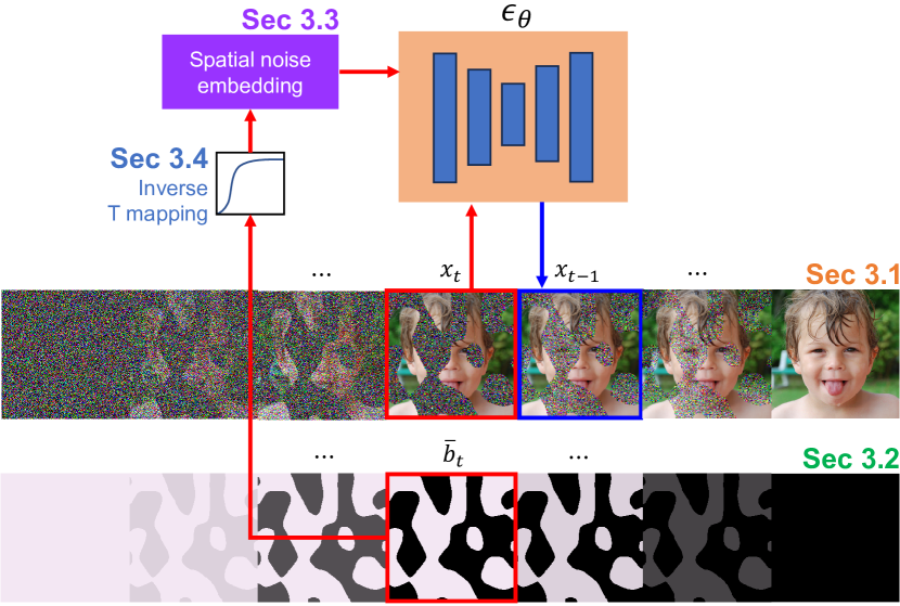
Figure 2: An overview of the proposed method. RAD consists of four components: (1) the forward and reverse processes based on pixel-wise noise (Section 3.1); (2) spatially variant noise schedules (Section 3.2); (3) spatial noise embedding (Section 3.3); and (4) the inverse-mapping of $\bar{b}$ (Section 3.4).

3 Region-Aware Diffusion Models

The core of the region-aware diffusion models (RADs) is redefining diffusion models so that each pixel has a different noise schedule, emulating inpainting scenarios. RADs define spatially variant noise schedules based on given masks (Sec. 3.2), which are utilized to establish both the forward and reverse processes based on pixel-wise noise (Sec. 3.1). This involves an element-wise reformulation of DDPM, of which many parts of the derivation naturally follow, however, there are some important points to consider (Secs. 3.3 and 3.4). This section will focus particularly on these critical points. The overview of RAD is shown in Figure 2.

3.1 Diffusion Models with Spatially Variant Noise

Here, we explain the basic framework of RAD, along with a brief explanation of DDPM [12]. The goal of a diffusion model is to learn to mimic a data distribution $q(x_{0})$, where $x_{0}$ denotes a ‘clean’ image without any noise, based on some model $p_{\theta}(x_{0})$ in an unsupervised manner. This is accomplished by learning an iterative denoising process that reverts a Brownian motion where $x_{0}$ gradually becomes pure Gaussian. This framework can be more tractable than directly learning $q(x_{0})$ because each individual task is to slightly denoise the noisy image at various noise stages.

Given a noise schedule, a sequence $x_{1},x_{2},\dots,x_{T}$ can be generated with some $T$ where the image gradually becomes noisier. The forward process governing this is defined as a Markov process with Gaussian transitions:

$$q\left(x_{1:T}|x_{0}\right)=\prod_{t\geq 1}q\left(x_{t}|x_{t-1}\right).$$ (1)

In DDPM, $q\left(x_{t}|x_{t-1}\right)=\prod_{i}q\left(x_{t,i}|x_{t-1,i}\right)$, $i$ denoting the element index, is assumed to be i.i.d. for the elements of $x_{t}$. At this point, RAD takes a different turn from DDPM, assuming the elements have different noise intensities:

$$q\left(x_{t,i}|x_{t-1,i}\right)=N\left(\sqrt{1-b_{t,i}}x_{t-1,i},\,b_{t,i}\,\right)$$ (2)

where $b_{t,i}$ is the variance of the $i$-th element of $x_{t}$ given $x_{t-1}$, i.e., the covariance matrix of $q\left(x_{t}|x_{t-1}\right)$ is $\text{diag}(b_{t})$. Similarly, the marginal distribution of $x_{t,i}$ can be given as

$$q\left(x_{t,i}|x_{0,i}\right)=N\left(\sqrt{\bar{a}_{t,i}}x_{0,i},1-\bar{a}_{t,i}\right)$$ (3)

with $a_{t,i}\triangleq 1-b_{t,i}$, $\bar{a}_{t,i}\triangleq\prod_{s=1}^{t}a_{s,i}$, and $\bar{b}_{t,i}\triangleq 1-\bar{a}_{t,i}$. This spatially variant noise assumption allows asynchronous generation of regions within the image, i.e., different regions can be subjected to different noise intensities so that the individual regions can be generated at different speeds, not affecting already generated ones. This alternate formulation, despite its simplicity, has proven to be quite effective in our experiments.

Even though the forward process is quite simply defined, the reverse process, i.e., the denoising process, has no closed-form solution. The essential reason is that the data distribution $q(x_{0})$ is not simple, and hence, the Bayes equation cannot be solved easily. Accordingly, we need to learn a model $p_{\theta}(x_{0})$ that approximates the reverse process. In diffusion models, $p_{\theta}(x_{0})$ is also formulated as a Markov process, starting from $x_{T}$, reversing the timesteps:

$$p_{\theta}\!\left(x_{0:T}\right)=p\!\left(x_{T}\right)\prod_{t\geq 1}p_{\theta}\!\left(x_{t-1}|x_{t}\right),$$ (4)

where $p\!\left(x_{T}\right)=N\!\left(0,I\right)$ is pure Gaussian noise. The reverse transition is also modeled as Gaussian, i.e., $p_{\theta}\!\left(x_{t-1}|x_{t}\right)=N\!\left(\mu_{\theta,t}\!\left(x_{t}\right),\text{diag}(s_{t})\right)$, however, the mean $\mu_{\theta,t}$ is a learnable function of $x_{t}$. In practice, the true $\mu_{t}$ of the denoising process can be expressed in terms of $x_{t}$ and the accumulated noise $\epsilon_{t}$ (in $x_{t}$), $\epsilon_{\theta}(x_{t},t)$ is learned to predict $\epsilon_{t}$ instead:

$$\mu_{\theta,t,i}\!\left(x_{t}\right)=\frac{1}{\sqrt{a_{t,i}}}\left(x_{t,i}-\frac{b_{t,i}}{\sqrt{1-\bar{a}_{t,i}}}\epsilon_{\theta,i}(x_{t},t)\right).$$ (5)

Again, this is an element-wise version that can include RAD, while all $a_{t,i}$, $b_{t,i}$, and $\bar{a}_{t,i}$ terms are identical for $i$ in DDPM, and the same goes for $s_{t}$ as well. In RAD, a division-by-zero can happen in the above equation, i.e., $\bar{a}_{t,i}=1$, if no noise has been added to the $i$-th pixel until $t$. In this case, a separate derivation gives $\mu_{\theta,t,i}=x_{t,i}$.

In the above, although the forward process in Eq. 1 has no spatial dependence, $p_{\theta}\!\left(x_{t-1}|x_{t}\right)$ surely has. This is because $q(x_{0})$ also likely has strong spatial dependence. Accordingly, $p_{\theta}$ must take the global context into account in the denoising process. This is why $\mu_{\theta,t,i}\!\left(x_{t}\right)$ and $\epsilon_{\theta,i}(x_{t},t)$ in (5), even though they indicate specific (the $i$-th) elements of $\mu_{\theta,t}$ and $\epsilon_{\theta}$, respectively, take the entire $x_{t}$ as an input.

Given the above forward and reverse processes, a variational loss can be defined as

This basically trains $p_{\theta}\!\left(x_{t-1}|x_{t}\right)$ to match the target $q\!\left(x_{t-1}|x_{t},x_{0}\right)$, except for $t=1$. In [12], a simpler loss has been proposed as

$$\begin{split}&L=\sum_{t\geq 1}\mathbb{E}_{q}\!\left[\left\|\epsilon_{t}-\epsilon_{\theta}(x_{t},t)\right\|^{2}\right],\end{split}$$ (7)

which directly trains $\epsilon_{\theta}$ to predict $\epsilon_{t}$. This has shown to be effective, and in many later works [23, 8], both (6) and (7) have been frequently used. In RAD, the calculation of (6) must be done with the element-wise versions of $q$ and $p_{\theta}$. After training, an image can be generated by performing a reverse process based on the learned $p_{\theta}$ from a randomly generated Gaussian noise.

As can be seen above, the basic framework of RAD is quite simple, i.e., an element-wise reformulation of DDPM. However, this is an easier part of RAD. For this framework to actually work, there are several important issues to consider: (i) What is an appropriate choice for the spatially variant noise ($b_{t}$)? (ii) How can $\epsilon_{\theta}$ successfully learn from the altered problem setting? (iii) How can we reduce additional efforts in training this alternate formulation? For the rest of the section, we will elaborate on the above points.

3.2 Generating Noise Schedules

Seeing RAD, one can quickly notice that the newly introduced flexibility requires careful attention. Unlike DDPM where a fixed noise schedule is applied to all pixels, those are set differently in RAD to allow asynchronous generation of different regions. These schedules must be somehow designed, and they must include various patterns during training so that diverse inpainting scenarios can be handled.

To encompass various noise shapes, we generate $b_{t}$ randomly during training. Now, the noise schedules also form a distribution, and the loss function (6) must include this in the expectation. In other words, we now have $q(x_{0:T}|b_{1:T})$ where $b_{1:T}$ follows some $q(b_{1:T})$. There are infinite choices for $q(b_{1:T})$, which becomes important since it can affect training. A naïve approach, such as selecting a random schedule for each pixel independently, can be problematic because the resulting noise may not have any distinctive spatial pattern, which is inconsistent with the actual inpainting scenarios. Indeed, this was not very successful in our empirical experience, meaning that having too random a noise pattern can be detrimental to the success of RAD.

Considering the above point, we limit the possible shapes of $b_{t}$ strictly to the inpainting scenarios. Specifically, we divide the entire diffusion process into two phases, where noise is filled in only for the pixels in a given inpainting mask in Phase 1 and the rest in Phase 2. This adequately represents an inpainting process, where only a part of an image is generated (Phase 1) while the other parts are already present (phase 2). The order of these phases is set in reverse order because the actual generation is performed in the reverse process. After training, only Phase 1 is utilized in inpainting because this suffices to generate the mask region. In fact, we may only utilize Phase 1 during training as well, but using both phases was better in our experience.

To mimic the noise-filling process of DDPM in each phase, we use the following strategy: Let $T_{1}$ and $T_{2}$ be the numbers of timesteps for Phases 1 and 2, respectively, i.e., $T_{1}+T_{2}=T$. During each phase, each pixel in or outside the mask is filled in by a scalar noise with variance $\beta_{t}$ ($1\leq t\leq T_{1}$) or $\beta_{t}^{\prime}$ ($1\leq t\leq T_{2}$), respectively, with $0<\beta_{t},\beta_{t}^{\prime}<1$. In practice, we use simple linear schedules for $\beta_{t}$ and $\beta_{t}^{\prime}$ as in DDPM. A caveat here is that all pixels must have the same accumulated noise levels after finishing the two phases, which can be satisfied easily by normalizing $\beta_{t}$ and $\beta_{t}^{\prime}$ as explained in the supplementary material. Gathering the above pixel-wise noise schedules, we can form $b_{t}$.

In the above strategy, the quality of inpainting masks during training is crucial. Unlike test conditions, numerous masks must be automatically supplied during training. Accessing the true mask distribution is not viable, so we need to find some sort of surrogate that includes diverse natural patterns mimicking real-world inpainting tasks. To this end, we propose to use Perlin noise [24]. Perlin noise, known for its smooth and naturalistic patterns, allows us to create diverse and realistic masks. To generate binary masks, we utilize black-and-white Perlin noise, which can be obtained by simple thresholding. We sample Perlin noise with various spatial scales by uniformly sampling the scale parameter so that the generated patterns have both finer and coarser structures. We also sample the black-and-white conversion threshold to control the overall area of inpainting. Figure 3 shows examples of generated masks. This surrogate distribution is quite effective, providing SoTA performance.

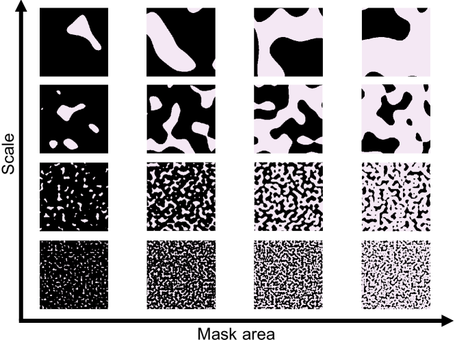
Figure 3: Examples of inpainting masks based on Perlin noise.

An interesting fact is that, even though there is a sharp separation between the mask and non-mask regions in the above strategy, the inpainting results do not exhibit any noticeable boundary effects. We have also tried blurring the boundaries of the masks, with no meaningful improvement in performance. This suggests that RAD is inherently capable of generating content adaptively to existing regions.

3.3 Spatial Noise Embedding

In diffusion models, a deep network $\epsilon_{\theta}(x_{t},t)$ is trained to estimate the accumulated noise $\epsilon_{t}$ in $x_{t}$. RAD does not have any structural difference in this regard, i.e., it shares the same input and output for $\epsilon_{\theta}$. In fact, RAD solves a more difficult problem than that of DDPM, because $\epsilon_{t}$ becomes more complicated. Hence, using this exact same structure might not be as successful as in DDPM, as also confirmed in our ablation study.

To resolve this issue, we focus on the $t$ input in $\epsilon_{\theta}(x_{t},t)$, which helps the network handle different steps adaptively. In practice, $t$ undergoes some embedding, comprising a cos-sin encoding and FC layers, and is added to every pixel of feature maps in the U-Net. Regarding this $t$ input, we conjecture that its main role is to inform $\epsilon_{\theta}$ of the overall intensity of $\epsilon_{t}$. This is somewhat reasonable because the intensity of $\epsilon_{t}$ increases as $t$ progresses in DDPM. Accordingly, we propose to use $\bar{b}_{t}$, the pixel-wise intensity of $\epsilon_{t}$ in RAD, in place of $t$ instead. This is easily accomplished by replacing the FC layers in the embedding module into $1\times 1$ convolutions. In this way, the pixel-wise noise condition can be directly informed to the network, making it easier to learn the spatially variant $\epsilon_{t}$. This actually works without changing any other component, confirming the above conjecture.

The above spatial noise embedding can be viewed as an indirect way of spatial conditioning, which has some similarities with conventional conditioning techniques. However, it is more subtle in that it alters the existing $t$ embedding and is completely determined by the noise schedules.

3.4 Practical Considerations

Although RAD has been explained in terms of DDPM, the proposed approach based on spatially variant noise is not limited to DDPM; it can be similarly applied to other advanced models such as DDIM [31], iDDPM [23], ADM [8], score-based models [32], and stable diffusion [27]. We have successfully tested RAD with many of these. For example, DDIM shares the same training procedure as DDPM, but differs in the reverse process, which we can also apply a similar element-wise reformulation. Similarly, iDDPM and ADM share the forward and reverse processes of DDPM but differ in the denoiser structures and loss functions, which combine (6) and (7). Hence, RAD can be extended to these without an issue, and all examples in the experiments are based on ADM versions. Since the basic framework of RAD is quite simple and universal, we expect it to work on other similar models as well.

One limitation of RAD is that the alternate formulation requires fresh training. Even though this is the reason for the superb generation speed compared to the existing SoTA methods, it can also be a deal-breaker considering the amount of resources required in training. This is why the most recent methods attempt to modify only the generation processes of pretrained models, sacrificing the speed. In this paper, we address this issue by utilizing LoRA [13], which can significantly reduce training efforts by leveraging pretrained models. To train RAD based on LoRA, some minor adjustment is required: The spatial noise embedding in RAD can be too drastic of a change for LoRA. Fortunately, the noise schedules for individual pixels are set to match that in DDPM, so we can inverse-map the elements of $\bar{b}_{t}$ to timestep values based on the accumulated noise levels in the steps of DDPM. We use linear interpolation in this process, meaning that the mapped timestep values can be non-integral. This has proven to be effective in the experiments, where all the examples are actually fine-tuned by LoRA based on pretrained ADMs. This approach makes RAD much more accessible.

In an actual implementation of RAD, singularities in the loss function must be carefully reviewed and avoided. In fact, there is a potential singularity in the variational loss (6), especially in the first step ($t=1$) where $p_{\theta}(x_{0}|x_{1})$ is prone to becoming degenerate. Even though DDPM uses the simplified loss (7) in practice, which has no singularities, later works such as iDDPM and ADM use both (6) and (7), where the singularities become a problem and are handled by some heuristics. This is an often-overlooked problem that can render training unstable, and for RAD, the issue is a little more complicated because the pixels undergo asynchronous noise schedules. The details are explained in the supplementary material.

4 Experiments

4.1 Benchmark Datasets

We validate RAD on the FFHQ [14], LSUN Bedroom [41], and ImageNet [7]. These datasets are well-suited for training and evaluating high-quality image generation models.

• FFHQ (Flickr-Faces-HQ) [14] contains a total of 70,000 high-resolution (1024x1024) images of human faces. This dataset provides greater diversity than traditional facial image datasets, encompassing a wide range of ages, genders, ethnicities, hairstyles, and accessories (e.g., glasses, hats, etc.). All images were resized to $256\times 256$.

• LSUN Bedroom [41] is a large-scale dataset of indoor scenes, containing over 3M bedroom images. Captured from various angles and perspectives, these images represent complex room structures, enabling algorithms to learn and generate intricate scene layouts. We train RAD with 288K samples of the LSUN Bedroom for convenience. All images were resized to $256\times 256$.

• ImageNet [7] is a large-scale image dataset for visual object recognition, containing over 1.2M labeled images across 1,000 categories. This dataset offers extensive diversity, covering a wide range of objects, animals, scenes, and complex visual compositions. All images were resized to $256\times 256$ for consistency in our experiments.

Table 1: Performance (FID and LPIPS) on FFHQ and LSUN Bedroom with various mask types. ^† indicates that the value is quoted from the original paper. Bold: best, under: second best.

Method	FFHQ						LSUN Bedroom
	Box		Extreme		Wide		Box		Extreme		Wide
	FID $\downarrow$	LPIPS $\downarrow$	FID $\downarrow$	LPIPS $\downarrow$	FID $\downarrow$	LPIPS $\downarrow$	FID $\downarrow$	LPIPS $\downarrow$	FID $\downarrow$	LPIPS $\downarrow$	FID $\downarrow$	LPIPS $\downarrow$
LaMa [33]	27.7†	0.086†	61.7†	0.492†	23.2†	0.096†	-	-	-	-	-	-
Score-SDE [32]	30.3†	0.135†	48.6†	0.488†	29.8†	0.132†	23.7	0.648	24.1	0.648	23.2	0.644
DDRM [15]	28.4†	0.109†	48.1†	0.532†	27.5†	0.113†	20.5	0.166	33.1	0.450	26.4	0.190
RePAINT [20]	25.7†	0.093†	35.9†	0.398†	24.2†	0.108†	20.5	0.176	23.5	0.461	21.4	0.161
MCG [4]	23.7†	0.089†	30.6†	0.366†	22.1†	0.099†	19.9	0.131	22.0	0.395	20.9	0.108
DDNM [34]	30.4	0.089	87.7	0.353	30.4	0.089	22.7	0.150	53.3	0.431	23.2	0.126
DeqIR [2]	24.2	0.093	64.2	0.368	27.4	0.099	22.2	0.176	43.9	0.461	22.0	0.153
RAD (ours)	22.1	0.074	33.4	0.317	21.5	0.078	19.2	0.131	21.6	0.399	20.8	0.107

Input	RePaint	MCG	RAD

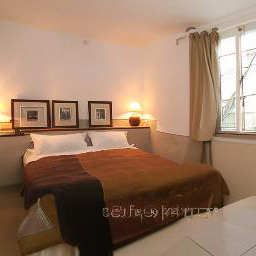
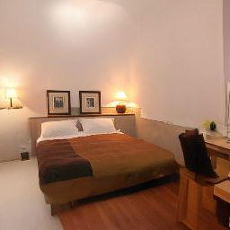
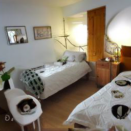
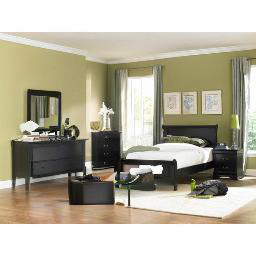
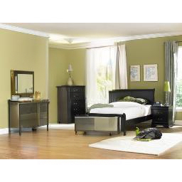
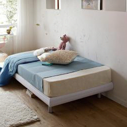
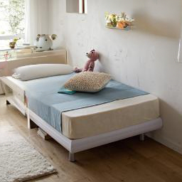
(a) LSUN Bedroom

Input	RePaint	MCG	RAD

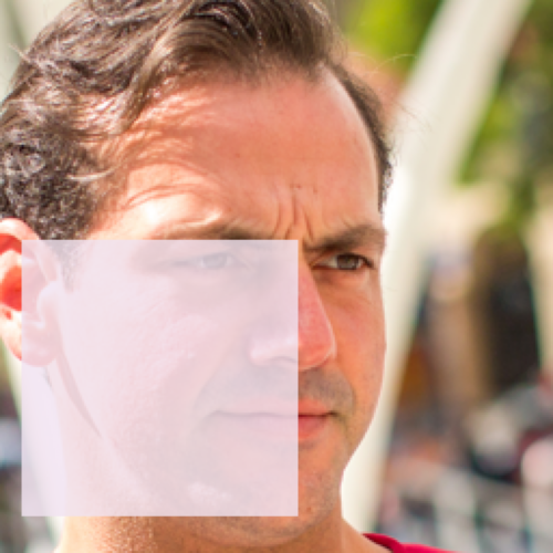
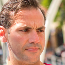
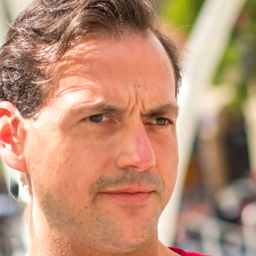
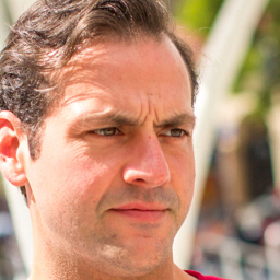
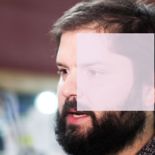
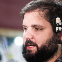
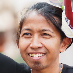
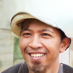
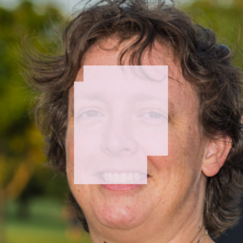
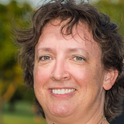
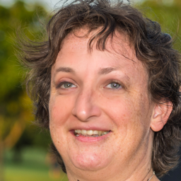
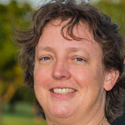
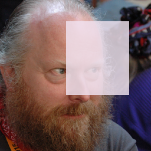
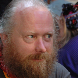
(b) FFHQ

Input	RePaint	MCG	RAD

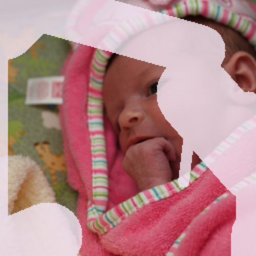
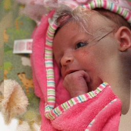
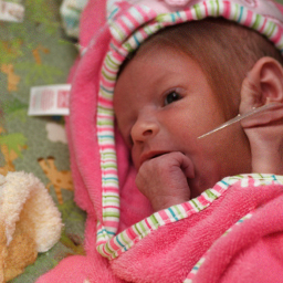
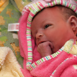
(c) ImageNet

Figure 4: Qualitative comparisons. Colored areas indicate inpainting regions (1st/2nd rows: box, 3rd/4th: extreme, 5th/6th: wide).

4.2 Implementation Details

Training settings.

For all experiments, we set the rank of LoRA [13] to 16 and trained RAD using the Adam optimizer [16] with a learning rate of $10^{-4}$. We used a batch size of 16 for both FFHQ and ImageNet, while that was eight for LSUN Bedroom. The total diffusion steps was 2000, with the initial 1000 steps dedicated to Phase 1. We used predefined linear noise schedules for $\beta_{t},\beta_{t}^{\prime}\in\left(0.0001,0.02\right)$. During inpainting, we used 100 sampling steps. FFHQ was trained on four TITAN RTX GPUs, LSUN Bedroom on eight NVIDIA 3090 GPUs, and ImageNet on eight NVIDIA RTX 6000 ADA GPUs. Pretrained ADM models [8] were used for all datasets. RAD was trained for 300K on FFHQ and LSUN Bedroom, and 800K on ImageNet.

Validation settings.

For validation, we set aside 1000 images from all datasets. We evaluated RAD across three types of mask configurations: box, extreme, and wide, following the practice in [33]. A box mask randomly removes a $128\times 128$ square region. In contrast, an extreme mask retains only a specific $128\times 128$ region, removing all other surrounding areas. A wide mask defines irregular missing regions. For inpainting, we used the reverse process of DDPM rather than DDIM due to its superior quality in generating realistic details.

Baseline.

We chose various inpainting methods based on GANs and diffusion models. For the GAN-based baseline, we used LaMA [33], and for the diffusion-based baselines, we employed RePaint [20], MCG [4], DDRM [15], DDNM [34], and DeqIR [2]. Publicly available pretrained ADM models [8] were used for all methods. Additionally, each method was evaluated using its publicly available codebase to maintain consistency in performance assessment.

Metrics.

To evaluate the performance of the proposed method and compare it with existing approaches, we employed Frechet Inception Distance (FID) [11] and the Learned Perceptual Image Patch Similarity (LPIPS) [43] as the inpainting quality measure.

4.3 Results

Comparisons.

Table 1 shows the inpainting performance of various methods. Reported values are either directly quoted from the original papers or computed by us if publicly available pretrained models exist. For LaMa, no pretrained model was available for LSUN Bedroom. Here, RAD achieves the best performance in terms of LPIPS and demonstrates superior FID scores for FFHQ and LSUN Bedroom compared to most baseline methods. Notably, DDNM and DeqIR exhibit relatively weaker performance in our experiments, even though they are relatively newer methods. The main goal of these methods is image restoration, and they are not specifically designed for challenging inpainting scenarios, particularly those involving large missing areas. Consequently, these methods show worse performance under our experimental settings. Figure 4 shows qualitative comparisons on LSUN Bedroom, FFHQ, and ImageNet. Here, all the methods are compared based on the same combinations of images and inpainting masks. The results confirm that RAD generally produces more natural images than others and has fewer failure cases.

Table 2 shows the inference time of various methods. We evaluated all methods on $256\times 256$ images using a single NVIDIA TITAN RTX GPU. Here, RAD is about 100 times faster than RePaint and 15 times faster than MCG while delivering superior performance. Baseline methods other than RePaint and MCG are much faster, but their inpainting quality is significantly worse.

Table 2: Inference time comparison ($1\times$ NVIDIA TITAN RTX).

Method	Inference time [s]
Score-SDE [32]	41.983
DDRM [15]	12.291
RePAINT [20]	837.136
MCG [4]	128.058
DDNM [34]	6.566
DeqIR [2]	26.443
Ours	8.442

Analysis of diversity.

Figure 5 demonstrates that RAD can generate diverse inpaintings across various mask configurations. Each row in the figure shows the input image with a specific mask, followed by multiple inpainting results (Samples 1 to 4) generated by RAD. These results highlight RAD’s ability to produce various plausible and contextually consistent inpaintings, even under challenging masks.

Input	Sample 1	Sample 2	Sample 3	Sample 4

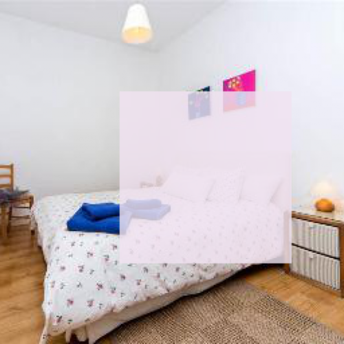
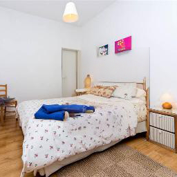
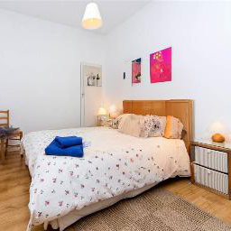
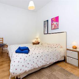
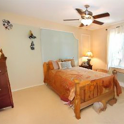
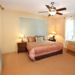
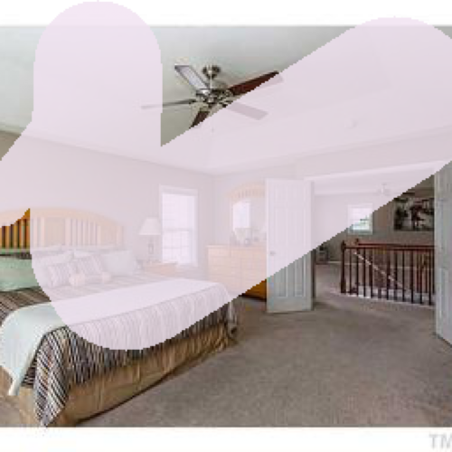
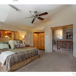
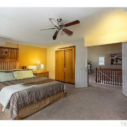
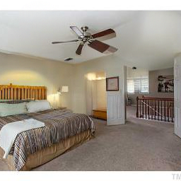
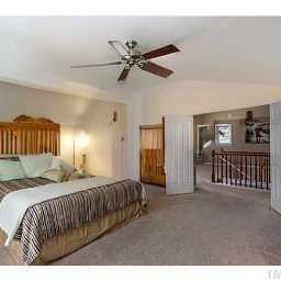
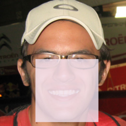
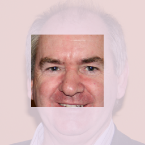
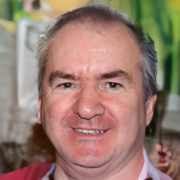
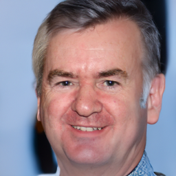
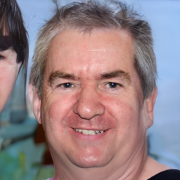
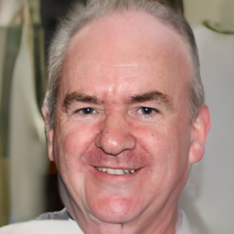
Figure 5: Example results of RAD on LSUN Bedroom and FFHQ.

Table 3: Ablation study of RAD on FFHQ (Cfg. 1: pretrained ADM with RAD reverse steps, Cfg. 2: w/o spatial noise emb.).

Method	Box		Extreme		Wide
	FID $\downarrow$	LPIPS $\downarrow$	FID $\downarrow$	LPIPS $\downarrow$	FID $\downarrow$	LPIPS $\downarrow$
Cfg. 1	128.3	0.279	172.0	0.441	95.7	0.240
Cfg. 2	23.5	0.086	37.0	0.333	26.8	0.085
RAD (ours)	22.1	0.074	33.4	0.317	21.5	0.078

Ablation study.

To verify the effectiveness of the proposed components, we compared RAD with two alternative methods: (1) performing RAD reverse steps directly on a pretrained ADM (i.e., no spatially variant noise training and no spatial noise embedding) and (2) RAD without spatial noise embedding (i.e., using $t$ embedding). As shown in Table 3, the RAD reverse steps do not perform well on a pretrained ADM model, which suggests that training with spatially variant noise is vital for RAD. Moreover, $t$ embedding exhibits inferior performance to spatial noise embedding in RAD, showing the effectiveness of the proposed embedding in inpainting tasks. This conclusion is further supported by qualitative results in Figure 6.

Input	Cfg. 1	Cfg. 2	RAD

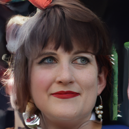
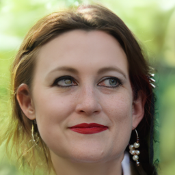
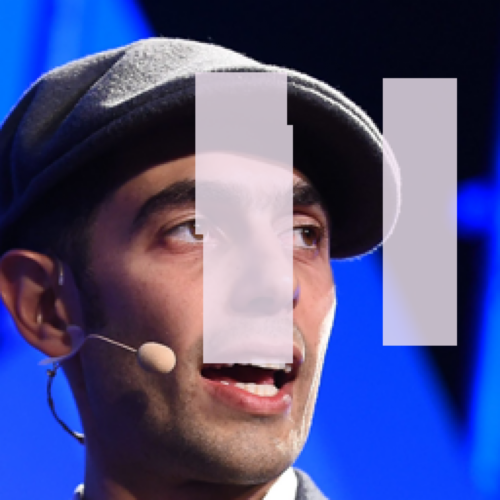
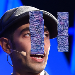
Figure 6: Ablation study examples on FFHQ (Cfg. 1: pretrained ADM with RAD reverse steps, Cfg. 2: w/o spatial noise emb.).

5 Limitations

A limitation of RAD is that it requires explicit training. The burden of training a diffusion model can be significant, and accordingly, we utilized LoRA to mitigate this issue greatly. Additionally, RAD is trained using a spatially variant noise schedule defined based on masks, making it dependent on the mask distribution. Perlin masks proposed in this paper are effective enough to handle most inpainting scenarios. However, there is a possibility that RePaint or MCG might yield better results in drastic cases even though they take much longer inference time.

6 Conclusion

We presented a novel inpainting model, RAD, which utilizes a spatially variant noise schedule to allow asynchronous generation of different regions. RAD handles inpainting by selectively adding noise to the regions specified by a given mask, followed by denoising those areas. This approach enables the selective generation of masked regions while preserving the others. The Perlin noise-based mask generation technique has been presented to generate realistic masks during training. Additionally, we proposed spatial noise embedding, significantly enhancing inpainting quality compared to conventional $t$ embedding. RAD can perform seamless inpainting without any additional module, and a plain reverse process is sufficient to produce high-quality results with orders of magnitude faster sampling speed.

While RAD is mainly described in the context of inpainting, the overall framework has broader implications. By extending the pseudo-targets of diffusion models (the denoising distributions) to spatially variant distributions, RAD offers more means to analyze and manipulate spatial interactions in diffusion models, opening interesting future research directions. Combining RAD with conditions such as text will extend the framework to image editing, a direction for future work.

References

- Avrahami et al. [2023] Omri Avrahami, Ohad Fried, and Dani Lischinski. Blended latent diffusion. ACM transactions on graphics (TOG), 42(4):1–11, 2023.
- Cao et al. [2024] Jiezhang Cao, Yue Shi, Kai Zhang, Yulun Zhang, Radu Timofte, and Luc Van Gool. Deep equilibrium diffusion restoration with parallel sampling. In Proceedings of the IEEE/CVF Conference on Computer Vision and Pattern Recognition, pages 2824–2834, 2024.
- Chen and Zhao [2024] Haiwei Chen and Yajie Zhao. Don’t look into the dark: Latent codes for pluralistic image inpainting. In Proceedings of the IEEE/CVF Conference on Computer Vision and Pattern Recognition, pages 7591–7600, 2024.
- Chung et al. [2022] Hyungjin Chung, Byeongsu Sim, and Jong Chul Ye. Improving diffusion models for inverse problems using manifold constraints. 2022.
- Corneanu et al. [2024] Ciprian Corneanu, Raghudeep Gadde, and Aleix M Martinez. Latentpaint: Image inpainting in latent space with diffusion models. In Proceedings of the IEEE/CVF Winter Conference on Applications of Computer Vision, pages 4334–4343, 2024.
- Couairon et al. [2023] Guillaume Couairon, Jakob Verbeek, Holger Schwenk, and Matthieu Cord. Diffedit: Diffusion-based semantic image editing with mask guidance. In ICLR 2023 (Eleventh International Conference on Learning Representations), 2023.
- Deng et al. [2009] Jia Deng, Wei Dong, Richard Socher, Li-Jia Li, Kai Li, and Li Fei-Fei. Imagenet: A large-scale hierarchical image database. In 2009 IEEE conference on computer vision and pattern recognition, pages 248–255. Ieee, 2009.
- Dhariwal and Nichol [2021] Prafulla Dhariwal and Alexander Nichol. Diffusion models beat gans on image synthesis. Advances in neural information processing systems, 34:8780–8794, 2021.
- Goodfellow et al. [2014] Ian Goodfellow, Jean Pouget-Abadie, Mehdi Mirza, Bing Xu, David Warde-Farley, Sherjil Ozair, Aaron Courville, and Yoshua Bengio. Generative adversarial nets. Advances in neural information processing systems, 27, 2014.
- Hertz et al. [2022] Amir Hertz, Ron Mokady, Jay Tenenbaum, Kfir Aberman, Yael Pritch, and Daniel Cohen-Or. Prompt-to-prompt image editing with cross attention control. arXiv preprint arXiv:2208.01626, 2022.
- Heusel et al. [2017] Martin Heusel, Hubert Ramsauer, Thomas Unterthiner, Bernhard Nessler, and Sepp Hochreiter. Gans trained by a two time-scale update rule converge to a local nash equilibrium. Advances in neural information processing systems, 30, 2017.
- Ho et al. [2020] Jonathan Ho, Ajay Jain, and Pieter Abbeel. Denoising diffusion probabilistic models. Advances in neural information processing systems, 33:6840–6851, 2020.
- Hu et al. [2021] Edward J Hu, Yelong Shen, Phillip Wallis, Zeyuan Allen-Zhu, Yuanzhi Li, Shean Wang, Lu Wang, and Weizhu Chen. Lora: Low-rank adaptation of large language models. arXiv preprint arXiv:2106.09685, 2021.
- Karras et al. [2019] Tero Karras, Samuli Laine, and Timo Aila. A style-based generator architecture for generative adversarial networks. In Proceedings of the IEEE/CVF conference on computer vision and pattern recognition, pages 4401–4410, 2019.
- Kawar et al. [2022] Bahjat Kawar, Michael Elad, Stefano Ermon, and Jiaming Song. Denoising diffusion restoration models. Advances in Neural Information Processing Systems, 35:23593–23606, 2022.
- Kingma and Ba [2015] Diederik P. Kingma and Jimmy Ba. Adam: A method for stochastic optimization. In International Conference on Learning Representations, San Diego, California, 2015.
- Kingma and Welling [2013] Diederik P Kingma and Max Welling. Auto-encoding variational bayes. arXiv preprint arXiv:1312.6114, 2013.
- Liu et al. [2018] Guilin Liu, Fitsum A Reda, Kevin J Shih, Ting-Chun Wang, Andrew Tao, and Bryan Catanzaro. Image inpainting for irregular holes using partial convolutions. In Proceedings of the European conference on computer vision (ECCV), pages 85–100, 2018.
- Liu et al. [2024] Haipeng Liu, Yang Wang, Biao Qian, Meng Wang, and Yong Rui. Structure matters: Tackling the semantic discrepancy in diffusion models for image inpainting. In Proceedings of the IEEE/CVF Conference on Computer Vision and Pattern Recognition, pages 8038–8047, 2024.
- Lugmayr et al. [2022] Andreas Lugmayr, Martin Danelljan, Andres Romero, Fisher Yu, Radu Timofte, and Luc Van Gool. Repaint: Inpainting using denoising diffusion probabilistic models. In Proceedings of the IEEE/CVF conference on computer vision and pattern recognition, pages 11461–11471, 2022.
- Meng et al. [2021] Chenlin Meng, Yutong He, Yang Song, Jiaming Song, Jiajun Wu, Jun-Yan Zhu, and Stefano Ermon. Sdedit: Guided image synthesis and editing with stochastic differential equations. In International Conference on Learning Representations, 2021.
- Nichol et al. [2021] Alex Nichol, Prafulla Dhariwal, Aditya Ramesh, Pranav Shyam, Pamela Mishkin, Bob McGrew, Ilya Sutskever, and Mark Chen. Glide: Towards photorealistic image generation and editing with text-guided diffusion models. arXiv preprint arXiv:2112.10741, 2021.
- Nichol and Dhariwal [2021] Alexander Quinn Nichol and Prafulla Dhariwal. Improved denoising diffusion probabilistic models. In International conference on machine learning, pages 8162–8171. PMLR, 2021.
- Perlin [1985] Ken Perlin. An image synthesizer. ACM Siggraph Computer Graphics, 19(3):287–296, 1985.
- Phung et al. [2023] Hao Phung, Quan Dao, and Anh Tran. Wavelet diffusion models are fast and scalable image generators. In Proceedings of the IEEE/CVF Conference on Computer Vision and Pattern Recognition (CVPR), pages 10199–10208, 2023.
- Poole et al. [2022] Ben Poole, Ajay Jain, Jonathan T Barron, and Ben Mildenhall. Dreamfusion: Text-to-3d using 2d diffusion. arXiv preprint arXiv:2209.14988, 2022.
- Rombach et al. [2022] Robin Rombach, Andreas Blattmann, Dominik Lorenz, Patrick Esser, and Björn Ommer. High-resolution image synthesis with latent diffusion models. In Proceedings of the IEEE/CVF conference on computer vision and pattern recognition, pages 10684–10695, 2022.
- Ronneberger et al. [2015] Olaf Ronneberger, Philipp Fischer, and Thomas Brox. U-net: Convolutional networks for biomedical image segmentation. In Medical image computing and computer-assisted intervention–MICCAI 2015: 18th international conference, Munich, Germany, October 5-9, 2015, proceedings, part III 18, pages 234–241. Springer, 2015.
- Saharia et al. [2022] Chitwan Saharia, William Chan, Saurabh Saxena, Lala Li, Jay Whang, Emily L Denton, Kamyar Ghasemipour, Raphael Gontijo Lopes, Burcu Karagol Ayan, Tim Salimans, et al. Photorealistic text-to-image diffusion models with deep language understanding. Advances in neural information processing systems, 35:36479–36494, 2022.
- Sohl-Dickstein et al. [2015] Jascha Sohl-Dickstein, Eric Weiss, Niru Maheswaranathan, and Surya Ganguli. Deep unsupervised learning using nonequilibrium thermodynamics. In International conference on machine learning, pages 2256–2265. PMLR, 2015.
- Song et al. [2020] Jiaming Song, Chenlin Meng, and Stefano Ermon. Denoising diffusion implicit models. arXiv preprint arXiv:2010.02502, 2020.
- Song et al. [2021] Yang Song, Jascha Sohl-Dickstein, Diederik P Kingma, Abhishek Kumar, Stefano Ermon, and Ben Poole. Score-based generative modeling through stochastic differential equations. In International Conference on Learning Representations, 2021.
- Suvorov et al. [2022] Roman Suvorov, Elizaveta Logacheva, Anton Mashikhin, Anastasia Remizova, Arsenii Ashukha, Aleksei Silvestrov, Naejin Kong, Harshith Goka, Kiwoong Park, and Victor Lempitsky. Resolution-robust large mask inpainting with fourier convolutions. In Proceedings of the IEEE/CVF winter conference on applications of computer vision, pages 2149–2159, 2022.
- Wang et al. [2023] Yinhuai Wang, Jiwen Yu, and Jian Zhang. Zero-shot image restoration using denoising diffusion null-space model. The Eleventh International Conference on Learning Representations, 2023.
- Wu et al. [2024] Jie Wu, Yuchao Feng, Honghui Xu, Chuanmeng Zhu, and Jianwei Zheng. Syformer: Structure-guided synergism transformer for large-portion image inpainting. In Proceedings of the AAAI Conference on Artificial Intelligence, pages 6021–6029, 2024.
- Xiao et al. [2022] Zhisheng Xiao, Karsten Kreis, and Arash Vahdat. Tackling the generative learning trilemma with denoising diffusion GANs. In International Conference on Learning Representations (ICLR), 2022.
- Xie et al. [2023] Shaoan Xie, Zhifei Zhang, Zhe Lin, Tobias Hinz, and Kun Zhang. Smartbrush: Text and shape guided object inpainting with diffusion model. In Proceedings of the IEEE/CVF Conference on Computer Vision and Pattern Recognition, pages 22428–22437, 2023.
- Yang et al. [2023a] Binxin Yang, Shuyang Gu, Bo Zhang, Ting Zhang, Xuejin Chen, Xiaoyan Sun, Dong Chen, and Fang Wen. Paint by example: Exemplar-based image editing with diffusion models. In Proceedings of the IEEE/CVF Conference on Computer Vision and Pattern Recognition, pages 18381–18391, 2023a.
- Yang et al. [2023b] Ruihan Yang, Prakhar Srivastava, and Stephan Mandt. Diffusion probabilistic modeling for video generation. Entropy, 25(10):1469, 2023b.
- Yi et al. [2023] Taoran Yi, Jiemin Fang, Guanjun Wu, Lingxi Xie, Xiaopeng Zhang, Wenyu Liu, Qi Tian, and Xinggang Wang. Gaussiandreamer: Fast generation from text to 3d gaussian splatting with point cloud priors. arXiv preprint arXiv:2310.08529, 2023.
- Yu et al. [2015] Fisher Yu, Ari Seff, Yinda Zhang, Shuran Song, Thomas Funkhouser, and Jianxiong Xiao. Lsun: Construction of a large-scale image dataset using deep learning with humans in the loop. arXiv preprint arXiv:1506.03365, 2015.
- Yu et al. [2019] Jiahui Yu, Zhe Lin, Jimei Yang, Xiaohui Shen, Xin Lu, and Thomas S Huang. Free-form image inpainting with gated convolution. In Proceedings of the IEEE/CVF international conference on computer vision, pages 4471–4480, 2019.
- Zhao et al. [2020] Lei Zhao, Qihang Mo, Sihuan Lin, Zhizhong Wang, Zhiwen Zuo, Haibo Chen, Wei Xing, and Dongming Lu. Uctgan: Diverse image inpainting based on unsupervised cross-space translation. In Proceedings of the IEEE/CVF conference on computer vision and pattern recognition, pages 5741–5750, 2020.
- Zhao and Lian [2024] Yiming Zhao and Zhouhui Lian. Udifftext: A unified framework for high-quality text synthesis in arbitrary images via character-aware diffusion models. In European Conference on Computer Vision, pages 217–233. Springer, 2024.
- Zhuang et al. [2023] Junhao Zhuang, Yanhong Zeng, Wenran Liu, Chun Yuan, and Kai Chen. A task is worth one word: Learning with task prompts for high-quality versatile image inpainting. arXiv preprint arXiv:2312.03594, 2023.