Liquidity Pools as Mean Field Games: A New Framework

Abstract

In this work, we present an innovative application of the probabilistic weak formulation of mean field games (MFG) for modeling liquidity pools in a constant product automated market maker (AMM) protocol in the context of decentralized finance. Our work extends one of the most conventional applications of MFG, which is the price impact model in an order book, by incorporating an AMM instead of a traditional order book. Through our approach, we achieve results that support the existence of solutions to the Mean Field Game and, additionally, the existence of approximate Nash equilibria for the proposed problem. These results not only offer a new perspective for representing liquidity pools in AMMs but also open promising opportunities for future research in this emerging field.

Keywords— Mean field games, Automated market makers, Decentralized finance, Liquidity pools, Approximate Nash equilibrium, Optimal control, Cryptocurrency market dynamics

1 Introduction

In recent years, we have witnessed growing excitement around cryptocurrencies and decentralized exchanges (DEX) based on blockchain technology. This trend has given rise to a new form of market-making known as "automated market makers" (AMMs), which has captured the attention of both academics and financial industry professionals. DEX trading volumes have experienced significant growth since 2020, as shown in the following Figure 1, peaking at over $200 billion in May 2021 during the cryptocurrency bull run. This surge marked a substantial increase from previous levels, reflecting heightened interest in decentralized finance. Post-peak, volumes fluctuated but remained robust, demonstrating the resilience and ongoing adoption of DEX platforms. Recent trends in 2023 and 2024 indicate a recovery and stabilization, with diverse platforms like Uniswap and PancakeSwap contributing significantly to the market.

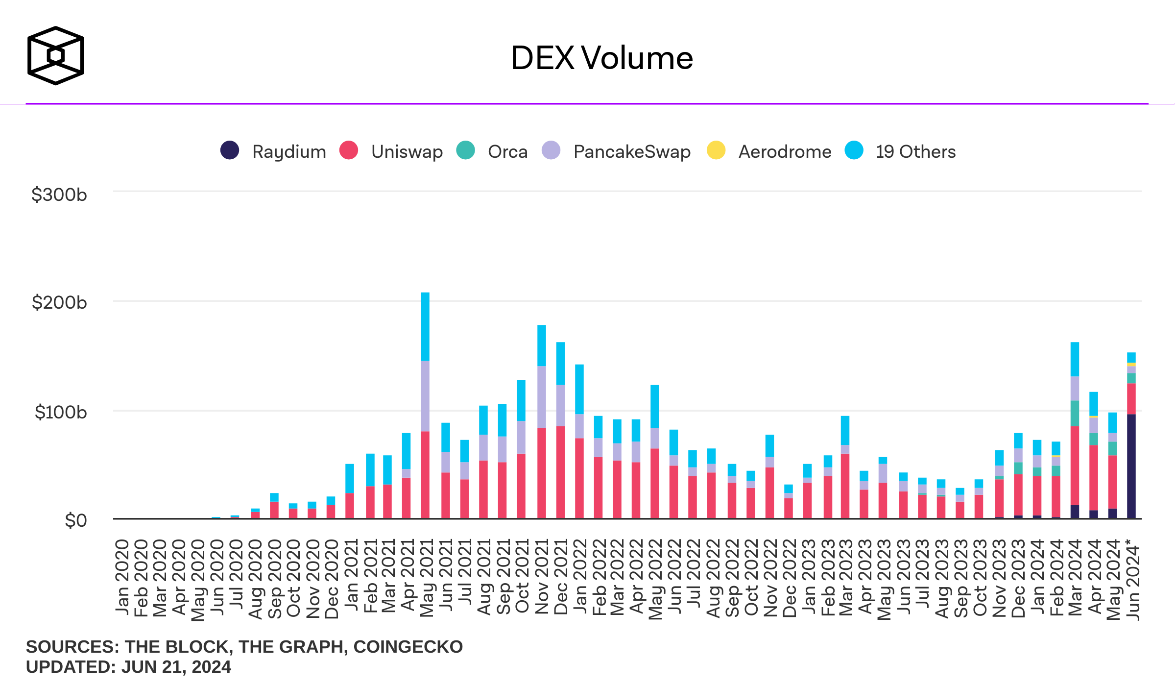
Source: The Block (The Block, The Graph, CoinGecko)

Figure 1: Monthly trading volume on DEXs.

A DEX is a cryptocurrency exchange platform with decentralized information management, based on blockchain technology. In these markets, price formation is carried out through algorithms known as AMMs. AMMs match trading orders and determine asset prices through a mathematical function called the "exchange function." Unlike traditional market-making protocols, such as order books, AMMs do not require the physical presence of market makers or intermediaries for order execution and price setting. In an automated market, traders do not trade directly with each other but transact with assets stored in an exchange, known as "liquidity pool". These liquidity pools are supplied by liquidity providers who wish to facilitate traders’ operations [4, 5, 14, 16].

Suppose that in a liquidity pool, exchanges of assets $X$ and $Y$ occur with initial reserves $x$ and $y$, respectively. When a trader buys an amount $\delta$ of tokens $Y$, paying a value of $p\delta$ in tokens $X$, this affects the pool’s reserves as follows: the value of token $Y$ in the pool decreases ($y_{0}\to y=y_{0}-\delta$), while the adjusted value in tokens $X$ increases ($x_{0}\to x=x_{0}+p\delta$). These changes in the pool’s reserves cause a transition from $(x_{0},y_{0})$ to $(x,y)$. In the particular case of a constant product AMM, it is required that the product of the liquidity pool’s reserves, excluding trading fees, remains constant, i.e., $k=xy=x_{0}y_{0}$ for some fixed value $k$. This equation determines the execution price $p$ for this transaction [2, 5, 14].

Mean field games (MFG) are a theoretical framework that describes strategic interaction in systems with a large number of agents who indirectly influence each other [1, 9, 13]. The MFG formalism focuses on studying interactions in scenarios where the actions of an individual agent have a negligible impact on the whole, but the collective significantly influences each agent’s outcome. This approach has found applications in diverse areas such as economics, engineering, biology, and, more recently, in the analysis of decentralized financial markets. MFGs allow modeling and predicting complex dynamics within these systems, facilitating the search for equilibria that represent stable states of the system under certain decision policies.

Typically, the equilibrium in MFGs is determined by the distribution of the agents’ states. However, in some economic applications, the cost faced by each agent depends on the distribution of the controls rather than the states, a framework known as "mean field games of controls" [8, 15, 7]. Our approach aligns with this framework, as the price discovery in the AMM is inherently linked to the aggregate actions of the traders, affecting the pool’s reserves and thus the price.

In a financial market, especially in the case of cryptocurrencies and digital assets, investors’ and traders’ decision-making can be highly strategic and influenced by a series of factors. The use of mean field game theory is justified in this context due to its ability to provide a robust framework that allows understanding how market participants interact in a decentralized environment and how their collective actions shape the overall market behavior. It was introduced independently by Lasry and Lions and by Huang, Malhamé, and Caines around 2006 [11, 10]. Since then, MFG has been extended to various domains, including price formation models [12, 6]. In traditional financial markets, these models typically treat demand as a function of price or vice versa. In contrast, our model leverages the unique structure of AMMs, where the price is a function of the liquidity reserves. This allows us to account for the direct impact of traders’ actions on price formation.

Our research builds upon the price impact model used in centralized markets, where order books typically serve as the exchange mechanism [3]. We adapt this model to address the control problem each trader faces when seeking to optimize their inventory while accounting for associated costs. However, unlike the traditional setup, our approach captures the price formation arising directly from the interaction of agents within the AMM, leveraging the unique characteristics of decentralized liquidity pools. We establish the existence of solutions to the mean field game and demonstrate the existence of approximate Nash equilibria, which provide a realistic extension to the classical Nash equilibrium concept by accommodating situations where exact equilibria are impractical to achieve. In this setting, an approximate Nash equilibrium is a state where no trader can significantly improve their outcome through a unilateral change in strategy, within a specified tolerance.

This paper advances the literature on AMMs and the use of bonding curves in DeFi by introducing a novel framework for applying mean field game theory to model liquidity pools. Our approach addresses the decentralized nature of AMMs by modeling the actions of "swappers" in a Uniswap v2-style liquidity pool without relying on probabilistic distributions for trader behavior. This direct modeling approach allows us to capture the strategic interactions among agents more accurately and provides new insights into equilibrium dynamics and decision-making processes in decentralized markets.

In Section 2 of this article, we will detail the inventory problem faced by a trader operating in a liquidity pool. We will explore the specific dynamics and constraints that influence these operators’ decision-making and conclude the section with a model for the price of the ETH asset in the liquidity pool.

In Section 3, we will apply the model results to the token price in the liquidity pool, analyzing its behavior and evaluating its impact in the context of the mean field game. Here, we will examine how market participants’ strategies and the dynamics of the liquidity pool influence price formation and decision-making.

Finally, in Section 4, we will present the conclusions derived from our study, summarizing the key findings, highlighting potential areas for improvement, and proposing future research that could expand and enrich the field of study. Our goal is to contribute to the understanding of cryptocurrency market dynamics and provide valuable insights for investors, traders, and academics interested in this exciting and dynamic field.

2 Model Formulation

We work with the filtered probability space $(\Omega,\mathcal{F}_{T},\mathbb{F},\mathbb{P})$ that supports $N+1$ uncorrelated Wiener processes $W_{0},\dotsm,W_{N}$.

We consider $N$ traders who trade their two tokens ETH and DAI in a liquidity pool. Let $X_{t}^{i}$ and $Y_{t}^{i}$ be the inventories of ETH and DAI, respectively, for the $i$-th trader at time $t$. The dynamics of the ETH inventory for the $i$-th trader are defined as

$$dX_{t}^{i}=\alpha_{t}^{i}dt+\sigma^{i}dW_{t}^{i},$$ (1)

where $\alpha_{t}^{i}:[0,T]\to\mathbb{R}$ represents the trading rate, these will be the controls; $\sigma^{i}$ represent the respective volatilities, which for simplicity we assume are independent of $i$; and $\sigma^{i}dW_{t}^{i}$ represents a random change in the trader’s inventory, associated with exogenous market events or inherent wallet usage.

On the other hand, the dynamics of the DAI inventory are

$$dY_{t}^{i}=-(\alpha_{t}^{i}P_{t}+c_{p}(\alpha_{t}^{i}))dt$$

where $P_{t}$ is the price at time $t$ of ETH in DAI units in the liquidity pool. The function $\alpha\to c_{p}(\alpha)$ models the cost for the trading rate $\alpha$ of trading in the pool.

For this first model, we will consider a liquidity pool given by a constant product AMM without transaction costs, i.e., $c_{p}\equiv 0$. Then, we have

$$P_{t}=\frac{Y_{t}}{X_{t}},$$

where $X_{t}$ and $Y_{t}$ are the balances in the pool of ETH and DAI, respectively. Furthermore, since the balances must satisfy the equation $X_{t}Y_{t}=k$ for all $t$, with $k$ constant and positive, we have

$$P_{t}=\frac{k}{X_{t}^{2}}.$$

According to the dynamics of ETH inventories for $N$ agents with $N\in\mathbb{N}$, we model the balance of ETH in the pool as follows

$$X_{t}:=X_{0}-\frac{1}{N}\sum_{i=1}^{N}\int_{0}^{t}\alpha_{s}^{i}ds,$$

where $X_{0}$ is the number of tokens provided by the liquidity provider at an initial time.

A detail to consider is that in a continuous-time trading model with multiple agents, it is unclear how simultaneous trades should be handled. More realistic are continuous-time discrete trading models. In the latter, it is reasonable to assume that agents never trade tokens simultaneously, given that there is a continuum of times to choose from.

In general, considering the average is a common practice in Mean Field Games theory, since when $N$ tends to infinity, the average tends to the empirical distribution of the controls.

A fundamental assumption is that $X_{t}\neq 0$ for all $t\in[0,T]$ because the pool must maintain at least a minimal fraction of tokens at all times. Therefore, we assume there exists $\epsilon_{0}>0$ such that

$$X_{t}\geq\epsilon_{0},\forall t.$$

Finally, the price of ETH is modeled as a martingale plus a drift that represents the permanent price impact

$$P_{t}:=\frac{k}{\left(X_{0}-\int_{0}^{t}\frac{1}{N}\sum_{i=1}^{N}\alpha_{s}^{i}ds\right)^{2}}+\sigma_{0}W_{t}^{0},$$

where $W_{t}^{0}$ is a Wiener process that models the inherent risks of the liquidity pool (slippage, illiquidity, oracle failures, exploits, etc.), and $\sigma_{0}$ is an associated volatility. Then,

$$dP_{t}=\frac{2k\frac{1}{N}\sum_{i=1}^{N}\alpha_{t}^{i}dt}{\left(X_{0}-\int_{0}^{t}\frac{1}{N}\sum_{i=1}^{N}\alpha_{s}^{i}ds\right)^{3}}+\sigma_{0}dW_{t}^{0}.$$

We consider the total inventory of the $i$-th trader at time $t$ with $V_{t}^{i}$ given by the sum of the DAI and ETH holdings in DAI units

$$V_{t}^{i}=Y_{t}^{i}+X_{t}^{i}P_{t}.$$

By Ito’s Lemma, we have

$$dV_{t}^{i} =dY_{t}^{i}+X_{t}^{i}dP_{t}+dX_{t}^{i}P_{t}$$ (2)

$$=\left[X_{t}^{i}\frac{2k\frac{1}{N}\sum_{i=1}^{N}\alpha_{t}^{i}}{\left(X_{0}-\int_{0}^{t}\frac{1}{N}\sum_{i=1}^{N}\alpha_{s}^{i}ds\right)^{3}}\right]dt$$

$$+X_{t}^{i}\sigma_{0}dW_{t}^{0}+P_{t}\sigma^{i}dW_{t}^{i}.$$

We assume the agents are risk-neutral and seek to maximize their expected profit from operating in the decentralized market, equivalently minimizing their trading cost. That is, the $i$-th trader seeks to maximize

$$J^{i}(\alpha^{1},\dots,\alpha^{N})=\mathbb{E}\left[V_{T}^{i}-\int_{0}^{T}h(t,X_{t}^{i})dt-l(X_{T}^{i})\right],$$

where $h:[0,T]\times\mathbb{R}\to\mathbb{R}$, $x\to h(t,x)$ represents the cost of maintaining an inventory $x$ at time $t$ and $l:\mathbb{R}\to\mathbb{R}$ represents a terminal inventory cost.

Remark.

Note that the mean field term in our problem appears in the form of the empirical distribution of the controls $\hat{q}_{t}^{N}=\frac{1}{N}\sum_{i=1}^{N}\alpha_{t}^{i}$, rather than being represented through the empirical distribution of the states, denoted by $\mu$ in the literature. However, in what follows, we will state the more general problem considering both distributions. The results will still hold for our model as it is a particular case of the general problem, where the involved functions are constant in the variable associated with the probability measure over the state space.

Working spaces

In what follows, we will define the spaces and functions involved in the previous mean field game to have the necessary context to use the results of [3].

• Let $\mathcal{C}:=C([0,T];\mathbb{R})$ be the space of continuous functions with values in $\mathbb{R}$ departing from $[0,T]$, equipped with the supremum norm $\|x\|:=\sup_{s\in[0,T]}|x(s)|$.

• Let $\Omega:=\mathbb{R}\times\mathcal{C}$.

• Define $\mathcal{F}_{t}$ as the completion of $\sigma((\xi,W_{s}):0\leq s\leq t)$ by $\mathbb{P}$-null sets of $\mathcal{B}(\Omega)$ and take $\mathbb{F}:=(\mathcal{F}_{t})_{0\leq t\leq T}$, where

  • $\mathbb{P}$ is the product of $\lambda_{0}$ and the Wiener measure, defined on $\mathcal{B}(\Omega)$, with $\lambda_{0}\in\mathcal{P}(\mathbb{R})$ the initial distribution of the infinite state processes of the players.

  • $\xi(x,\omega):=x$ and $W(x,\omega):=\omega$.

• Given $\mathcal{P}(\Omega)$, the space of probability functions over $\Omega$, and a measurable function $\psi:\mathcal{C}\to\mathbb{R}$, define

  $$\mathcal{P}_{\psi}(\Omega)=\left\{\mu\in\mathcal{P}(\Omega):\int\psi d\mu<\infty\right\},$$

  Define $\tau_{\psi}(\Omega)$ as the weakest topology on $\mathcal{P}_{\psi}(\Omega)$ that makes the map $\mu\to\int fd\mu$ continuous for each $f\in\mathcal{B}_{\psi}(\Omega)$.

• Let the control space $A\subset\mathbb{R}$ be a bounded subset and let $\mathbb{A}=\{\alpha:[0,T]\times\Omega\to A:\text{progressively measurable}\}$ be the set of admissible controls.

• Finally, let $\mathcal{P}(A)$ be the space of probability functions over $A$ along with the weak topology $\tau(A)$ that makes the map $q\to\int_{A}fdq$ continuous for each $f\in\mathcal{B}(A)$.

Then $J$ is written as

$$J^{i}(\alpha^{1},\dots,\alpha^{N})=\mathbb{E}\left[\int_{0}^{T}f(t,X_{t}^{i},\mu,\hat{q}_{t}^{N},\alpha_{t}^{i})dt-l(X_{T}^{i})\right],$$

where $\mu$ is a probability measure on the state space, $\hat{q}_{t}^{N}$ denotes the empirical distribution of $\alpha_{t}^{1},\dots,\alpha_{t}^{N}$, and by equation (2), the function $f:[0,T]\times\mathcal{C}\times\mathcal{P}_{\psi}(\Omega)\times\mathcal{P}(A)\times A\to\mathbb{R}$ is defined by

$$f(t,x,\mu,q,\alpha)=x_{t}\frac{2k\int\alpha dq}{\left(x_{0}-\int_{0}^{t}\int\alpha dq\right)^{3}}-h(t,x_{t}).$$

Intuitively, if $N$ is large, due to the symmetry of the model, the contribution of player $i$ to the empirical distribution of controls $\hat{q}_{t}^{N}$ is negligible, and $\hat{q}_{t}^{N}$ can be treated as fixed. We consider the limit when the number of agents $N$ tends to infinity, which simplifies the analysis by reducing the impact of individual fluctuations and focusing on the mean dynamics. Formally, we study the behavior of

$$J^{\mu,q}(\alpha):=\lim_{N\to\infty}J^{i}(\alpha^{1},\dots,\alpha^{N})=\mathbb{E}^{\alpha}\left[\int_{0}^{T}f(t,X,\mu,q_{t},\alpha_{t})dt-l(X_{T}^{i})\right],$$

where $q=\lim_{N\to\infty}\hat{q}_{t}^{N}$ is the limit of the empirical distribution of the controls.

Mean field game

We state the mean field game problem given by the following structure:

1. Fix a probability measure $\mu$ on the state space and a flow $q:t\to q_{t}$ of measures on the control space $\mathcal{P}(A)$;

2. With $\mu$ and $q$ fixed, solve the standard optimal control problem:

   $$\left\{\begin{array}[]{lcc}\sup_{\alpha}\mathbb{E}\left[\int_{0}^{T}f(t,X,\mu_{t},q_{t},\alpha_{t})dt-g(X,\mu)\right]&\text{s.t.}\\ dX_{t}=b(t,x,\mu,\alpha_{t})dt+\sigma dW_{t},&X_{0}=\xi\end{array}\right.$$ (3)

   where $f:[0,T]\times\mathcal{C}\times\mathcal{P}_{\psi}(\mathcal{C})\times\mathcal{P}(A)\times A\to\mathbb{R}$, $g:\mathcal{C}\times\mathcal{P}(\mathcal{C})\to\mathbb{R}$ and $b:[0,T]\times\mathcal{C}\times\mathcal{P}_{\psi}(\mathcal{C})\times A\to\mathbb{R}$.

3. Find an optimal control $\alpha$, incorporate it into the state dynamics $X$, and find the law $\Phi_{X}(\mu,q)$ of the optimally controlled state process, and the flow $\Phi_{\alpha}(\mu,q)$ of the marginal laws of the optimal control process;

4. Find a fixed point $\mu=\Phi_{X}(\mu,q)$, $q=\Phi_{\alpha}(\mu,q)$.

This should be interpreted as the optimization problem faced by a single representative player in a game consisting of an infinite number of independently and identically distributed (i.i.d.) players. In the first three steps, the representative player determines their best response to the states and controls of the other players, which they treat as given. The final step is an equilibrium condition; if each player takes this approach, and there must be some consistency, then there must be a fixed point. Once the existence and, perhaps, the uniqueness of a fixed point are established, the second problem is to use this fixed point to construct approximate Nash equilibrium strategies for the original finite-player game. These strategies will be constructed from the optimal control for the problem in step (2), corresponding to the choice $(\mu,q)$ being the fixed point in step (1).

Solution to the mean field game

We formalize what we mean by a solution to the MFG. Before that, we must specify the spaces we will work with.

Let $t\in[0,T]$, $\mathbb{P}\in\mathbb{P}(\Omega)$ be a probability measure on $\Omega:=\mathbb{R}\times\mathcal{C}$, and $q_{t}\in\mathbb{P}(A)$ be a probability measure on $A$. Given $\alpha\in\mathbb{A}$ and $X$ a $\mathcal{C}$-valued stochastic process, we can think of

$$\alpha_{t}:\Omega\to A,\omega \mapsto\alpha_{t}(\omega),$$

$$X:\Omega\to\mathcal{P}(\mathcal{C}),\omega \mapsto X_{\omega}=\{X_{t}(\omega)\}_{t\in[0,T]}$$

Then, given measurable sets $a\in\mathcal{P}(A)$ and $c\in\mathcal{P}(\mathcal{C})$, we have

$$\alpha_{t}^{-1}(a) =\{\omega\in\Omega:\alpha_{t}(\omega)\in a\},$$

$$X^{-1}(c) =\{\omega\in\Omega:X_{\omega}\subset c\}$$

We can think that $\alpha^{-1}(a)$ returns the events $\omega$ for which the image of $\alpha$ falls in $a$. We interpret this as the ”events induced by $\alpha$” (i.e., the law or distribution of $\alpha$); and that $X^{-1}(c)$ returns the events $\omega$ for which the paths drawn by $X_{\omega}$ are contained in $c$. We can think of ”events induced by $X$” (i.e., the law or distribution of $X$).

For each $\mu\in\mathcal{P}_{\psi}(\mathcal{C})$ and $\alpha\in\mathbb{A}$, a measure $\mathbb{P}^{\mu,\alpha}$ on $(\Omega,\mathbb{F}_{T})$ is defined by

$$\frac{dP^{\mu,\alpha}}{dP}=\mathcal{E}\left(\int_{0}^{\cdot}\sigma^{-1}b(t,X,\mu,\alpha_{t})dW_{t}\right)_{T}.$$

By Girsanov’s theorem and the boundedness of $\sigma^{-1}b$, the process $W^{\mu,\alpha}$ defined by

$$W_{t}^{\mu,\alpha}:=W_{t}-\int_{0}^{t}\sigma^{-1}b(s,X,\mu,\alpha_{s})ds$$

is a Wiener process under $\mathbb{P}^{\mu,\alpha}$, and

$$dX_{t}=b(t,X,\mu,\alpha)dt+\sigma dW_{t}^{\mu,\alpha}.$$

That is, under $\mathbb{P}^{\mu,\alpha}$, $X$ is a weak solution to the state equation. Note that $\mathbb{P}^{\mu,\alpha}$ and $\mathbb{P}$ are equal on $\mathcal{F}_{0}$; in particular, the law of $X_{0}=\xi$ remains $\lambda_{0}$. Moreover, $\xi$ and $W$ remain independent under $\mathbb{P}^{\mu,\alpha}$.

Then $\mathbb{P}^{\mu,\alpha}\circ X^{-1}=\mu$ and $\mathbb{P}^{\mu,\alpha}\circ\alpha_{t}^{-1}=q_{t}$ is asking that the events induced by $\alpha$ be the same as those identified by $q_{t}$; and $\mathbb{P}^{\mu,\alpha}\circ\alpha_{t}^{-1}=q_{t}$ is asking that the events induced by $X$ be the same as those identified by $\mu$.

We take a measure $\mu\in\mathcal{P}_{\psi}(\mathcal{C})$, a control $\alpha\in\mathbb{A}$, and a measurable map $t\in[0,T]\to q_{t}\in\mathcal{P}(A)$, we define the associated expected reward by

$$J^{\mu,q}(\alpha):=\mathbb{E}^{\mu,\alpha}\left[\int_{0}^{T}f(t,X,\mu,q_{t},\alpha_{t})dt+g(X,\mu)\right],$$

where $\mathbb{E}^{\mu,\alpha}$ denotes the expectation with respect to the measure $\mathbb{P}^{\mu,\alpha}$. Given $\mu$ and $q$ fixed, we face a standard stochastic optimal control problem, whose value is given by

$$V^{\mu,q}=\sup_{\alpha\in\mathbb{A}}J^{\mu,q}(\alpha).$$

Formally, we define a solution to the MFG as follows

Definition 2.1.

We say that a measure $\mu\in\mathcal{P}_{\psi}(\mathcal{C})$ and a measurable function $q:[0,T]\to\mathcal{P}(A)$ form a solution of the MFG if there exists $\alpha\in\mathbb{A}$ such that $V^{\mu,q}=J^{\mu,q}(\alpha)$, $\mathbb{P}^{\mu,\alpha}\circ X^{-1}=\mu$, and $\mathbb{P}^{\mu,\alpha}\circ\alpha_{t}^{-1}=q_{t}$ for almost every $t$.

3 Application

We will now prove the existence of a MFG solution for the token price model in a liquidity pool with infinite traders and, additionally, find approximate Nash equilibria when the pool operates with a finite number of traders.

Suppose $A\subset\mathbb{R}$ is a compact interval containing the origin, $\sigma>0$, $h:[0,T]\times\mathbb{R}\to\mathbb{R}$ and $l:\mathbb{R}\to\mathbb{R}$ are measurable, and finally that there exists $c_{1}>0$ such that

$$|h(t,x)|+|l(x)|\leq c_{1}e^{c_{1}|x|}\hskip 8.5359pt\text{ for all }(t,x)\in[0,T]\times\mathbb{R}.$$ (4)

We assume that $X_{0}^{i}$ are i.i.d and have a common distribution $\lambda_{0}\in\mathcal{P}(\mathbb{R})$ satisfying $\int_{\mathbb{R}}e^{p|x|}\lambda_{0}(dx)<+\infty$ for all $p>0$. With the notation of the previous sections, we have that if $(t,x,\mu,q,a)\in[0,T]\times\mathcal{C}\times\mathcal{P}_{\psi}(\mathcal{C})\times\mathcal{P}(A)\times A$, then we define the following functions:

$$b(t,x,\mu,a) :=a$$

$$f(t,x,\mu,q,a) :=x_{t}\frac{2k\int_{A}rdq_{t}(r)}{(x_{0}-\int_{0}^{t}\int_{A}rdq_{s}(r)ds)^{3}}-h(t,x_{t})$$

$$g(\mu,x) :=l(x_{T})$$

$$\psi(x_{t}) :=e^{c_{1}|x_{t}|}$$

Let us see that the hypotheses of Th. 3.5 from [3] are satisfied, which guarantees the existence of a MFG solution:

Corollary 3.1.

The following conditions are satisfied:

1. The control space $A$ is a compact and convex subset of $\mathbb{R}$ and the drift $b:[0,T]\times\mathcal{C}\times\mathcal{P}_{\psi}(\mathcal{C})\times A\to\mathbb{R}$ is continuous.

2. There exists a strong solution $X$ to the driftless state equation

   $$dX_{t}=\sigma dW_{t},\hskip 14.22636ptX_{0}=\xi,$$ (5)

   such that $\mathbb{E}[\psi^{2}(X)]<+\infty$, $\sigma>0$, and $\sigma^{-1}b(a)$ is uniformly bounded.

3. The cost/benefit function $f:[0,T]\times\mathcal{C}\times\mathcal{P}_{\psi}(\mathcal{C})\times\mathcal{P}(A)\times A\to\mathbb{R}$ is such that $(t,x)\to f(t,x,\mu,q,a)$ is progressively measurable for each $(\mu,q,a)$ and $a\to f(t,x,q,a)$ is continuous for each $(t,x,\mu,q)$. The terminal cost/reward function $g:\mathcal{C}\times\mathcal{P}_{\psi}(\mathcal{C})\to\mathbb{R}$ is Borel measurable for each $\mu$.

4. There exists $c>0$ such that

   $$|g(x,\mu)|+|f(t,x,\mu,q,a)|\leq c\psi(x)\hskip 5.69046pt\forall(t,x,\mu,q)\in[0,T]\times\mathcal{C}\times\mathcal{P}_{\psi}(\mathcal{C})\times\mathcal{P}(A).$$

5. The function $f$ is of the form

   $$f(t,x,\mu,q,a)=f_{1}(t,x,\mu,a)+f_{2}(t,x,\mu,q).$$

Proof.

Let us verify each of the above statements one by one.

1. The quantities of tokens traded by the agents cannot be infinite since $A$ is bounded, i.e., there exists $M$ such that $|\alpha(t,\omega)|\leq M,\forall(t,\omega)\in[0,T]\times\Omega$. We consider the control space $A$ as a closed interval containing the origin, therefore it is compact and convex. The drift is a continuous function, as it is the identity.

2. The function $\sigma^{-1}b(a)=\sigma^{-1}a$ is uniformly bounded since $A$ is compact. Moreover, since $\psi_{0}(x)=e^{p|x|}$, $\lambda_{0}$ is such that $\int_{\mathbb{R}^{d}}\psi_{0}(x)^{2}\lambda_{0}(dx)<\infty$ and $\sigma$ is constant, the hypotheses of Lemma 5.2 from [3] are verified.

For (S.3) and (S.4), observe that:

Remark.

• To ensure the model is well-posed, we assumed there exists $\epsilon_{0}>0$ such that $X_{t}\geq\epsilon_{0},\forall t\in\mathbb{R}$. Then,

  $$X_{0}-\int_{0}^{t}\int_{A}rdq_{s}(r)ds \geq X_{0}-\left(\max_{a\in A}|a|\right)\int_{0}^{t}\int_{A}1dq_{s}(r)ds=X_{0}-\left(\max_{a\in A}|a|\right)t.$$

  It suffices to require that the set of admissible controls be such that

  $$\left(\max_{a\in A}|a|\right)<\frac{X_{0}-\epsilon_{0}}{T}$$

• Using the above, we have

  $$\left|\frac{2k\int_{A}rdq_{t}(r)}{(X_{0}-\int_{0}^{t}\int_{A}rdq_{s}(r)ds)^{3}}\right| \leq\frac{2k\left(\max_{a\in A}|a|\right)}{\epsilon_{0}^{3}}$$

1. The function $f(t,x,\mu,q,a)=x\frac{2k\int_{A}rdq_{t}(r)}{(X_{0}-\int_{0}^{t}\int_{A}rdq_{s}(r)ds)^{3}}-h(t,x)$ is progressively measurable as a function of $(t,x)$ since it is well-defined and continuous, and is continuous as a function of $a$ since it is constant. Furthermore, the terminal cost $g(x,\mu)$ is continuous and hence Borel measurable.

2. By equation (4), we have

   $$|h(t,x)|+|l(x)|\leq c_{1}e^{c_{1}|x|}\hskip 8.5359pt\text{ for all }(t,x)\in[0,T]\times\mathbb{R},$$

   then if $x\in\mathcal{C}$,

   $$|g(x,\mu)+f(t,x,\mu,q,a)|\leq c_{1}e^{c_{1}|x|}+|x_{t}|\frac{2k\left(\max_{a\in A}|a|\right)}{\epsilon_{0}^{3}}\leq\tilde{c}e^{\tilde{c}|x|}$$

   for $\tilde{c}=\max\left\{c_{1},\frac{2k\left(\max_{a\in A}|a|\right)}{\epsilon_{0}^{3}}\right\}$. We have what we wanted for $\psi(x)=e^{\tilde{c}|x|}$.

3. Note that $f(t,x,\mu,q,a)=f_{1}(t,x,\mu,a)+f_{2}(t,x,\mu,q)$ where $f_{1}(t,x,\mu,a)=0$ and $f_{2}(t,x,\mu,q)=x\frac{2k\int_{A}rdq_{t}(r)}{(X_{0}-\int_{0}^{t}\int_{A}rdq_{s}(r)ds)^{3}}-h(t,x)$.

∎

Some additional conditions are needed for the existence results. The Hamiltonian $h:[0,T]\times\mathcal{C}\times\mathcal{P}_{\psi}(\mathcal{C})\times\mathcal{P}(A)\times\mathbb{R}^{d}\times A\to\mathbb{R}$, the maximized Hamiltonian $H:[0,T]\times\mathcal{C}\times\mathcal{P}_{\psi}(\mathcal{C})\times\mathcal{P}(A)\times\mathbb{R}^{d}\to\mathbb{R}$, and the set where the supremum is attained are defined by

$$h(t,x,\mu,q,z,a) =f(t,x,\mu,q,a)+z\sigma^{-1}b(t,x,\mu,a),$$

$$H(t,x,\mu,q,z) :=\sup_{a\in A}h(t,x,\mu,q,z,a),$$

$$A(t,x,\mu,q,z) :=\{a\in A:h(t,x,\mu,q,z,a)=H(t,x,\mu,q,z)\},$$

respectively. Note that by assumption (S.5), $A(t,x,\mu,q,z)$ does not depend on $q$, so we will use the notation $A(t,x,\mu,z)$. Furthermore, by assumptions (S.1) and (S.3), the compactness of $A$ and the continuity of $h$ in the variable $a$, we have that $A(t,x,\mu,z)$ is non-empty.

Corollary 3.2.

The following condition holds:

(C)

For each $(t,x,\mu,z)$, the set $A(t,x,\mu,z)$ is convex.

Proof.

It holds whenever $b$ is affine as a function of $a$ and $f$ is also concave as a function of $a$. The first condition follows from $b(a)=a$; the second because it is constant. ∎

It will be useful to have a notation for the law without drift and the set of equivalent laws,

$$\mathcal{X} :=\mathbb{P}\circ X^{-1}\in\mathcal{P}_{\psi}(\mathcal{C})$$

$$\mathcal{P}_{X} :=\{\mu\in\mathcal{P}_{\psi}(\mathcal{C}):\mu\sim\mathcal{X}\}$$

Corollary 3.3.

The following holds:

(E)

For each $(t,x)\in[0,T]\times\mathcal{C}$, the following maps are sequentially continuous, using $\tau_{\psi}(\mathcal{C})$ on $\mathcal{P}_{X}$ and the weak topology on $\mathcal{P}(A)$:

$$\mathcal{P}_{X}\times A \ni(\mu,a)\mapsto b(t,x,\mu,a),$$

$$\mathcal{P}_{X}\times\mathcal{P}(A)\times A \ni(\mu,q,a)\mapsto f(t,x,\mu,q,a),$$

$$\mathcal{P}_{X} \ni\mu\to g(x,\mu)$$

Proof.

For each $(t,x)\in[0,T]\times\mathcal{C}$, we have that $a\mapsto b(\mu,a)=a$ is sequentially continuous since it is continuous. Additionally, given that $q\mapsto\int_{A}rdq(r)$ is continuous, the map $(\mu,q,a)\mapsto f(t,x,\mu,q,a)=x_{t}\frac{2k\int_{A}rdq_{t}(r)}{(X_{0}-\int_{0}^{t}\int_{A}rdq_{s}(r)ds)^{3}}-h(t,x_{t})$ is also continuous. Finally, $g$ is constant with respect to $\mu$. ∎

Proposition 3.4.

There exists a solution to the MFG.

Proof.

By theorem Th. 3.5 from [3], since conditions (S) and (E) are satisfied, there exists a solution to the MFG. ∎

The failure to satisfy the necessary assumptions for uniqueness results (Th. 3.8, [3]) does not imply its inexistence; rather, it indicates that our model does not fit these specific hypotheses. It would be necessary to adjust the existing model or explore new results to address this discrepancy.

4 Approximation to Nash

We define the empirical measure map $e_{n}:\Omega^{n}\to\mathcal{P}(\Omega)$ by

$$e_{n}(\omega_{1},...,\omega_{n})=\frac{1}{n}\sum_{j=1}^{n}\delta_{\omega_{j}}$$

Definition 4.1.

Given the measurable spaces $E$ and $F$, we say that a function $f:\mathcal{P}(\Omega)\times E\to F$ is empirically measurable if

$$(x,y)\in\Omega^{n}\times E\to f(e_{n}(x),y)\in F$$

is jointly measurable for all $n\geq 1$.

Corollary 4.2.

The following hypotheses are satisfied:

1. The drift $b=b(t,x,a)$ has no mean field term.

2. The functions $b$, $f$, and $g$ are empirically measurable using the progressive $\sigma$-field on $[0,T]\times\mathcal{C}$ and the Borel $\sigma$-fields elsewhere.

3. For each $(t,x)$, the following functions are continuous at each point satisfying $\mu\sim\mathcal{X}$:

   $$\mathcal{P}_{\psi}(\mathcal{C})\times\mathcal{P}(A)\times A\ni(\mu,q,a)\mapsto f(t,x,\mu,q,a),$$

   $$\mathcal{P}_{\psi}(\mathcal{C})\ni\mu\to g(x,\mu);$$

4. There exists $c>0$ such that, for all $(t,x,q,a)$,

   $$|g(x,\mu)|+|f(t,x,\mu,q,a)|\leq c\left(\psi(x)+\int\psi d\mu\right).$$

Proof.

Note that (F.1) is clear. Let $E=[0,T]\times\mathcal{C}\times\mathcal{P}(A)\times A$ and let $(\vec{x},t,x,q,a)\in\mathcal{C}^{n}\times E$. We want to see that

$$(\vec{x},t,x,a) \mapsto b(t,x,e_{n}(\vec{x}),a),$$

$$(\vec{x},t,x,q,a) \mapsto f(t,x,e_{n}(\vec{x}),q,a),$$

$$(\vec{x},x) \mapsto g(x,e_{n}(\vec{x}))$$

are measurable, where $\vec{x}\in\mathcal{C}^{n}\mapsto e_{n}(\vec{x}):=\frac{1}{n}\sum_{i=1}^{n}\delta_{x_{i}}\in\mathcal{P}_{\psi}(\mathcal{C})$.

Since $b$ and $g$ in our case do not depend on the state law coordinate and are continuous, particularly measurable, and we are considering the progressive $\sigma$-fields on $[0,T]\times\mathcal{C}$ and the Borel $\sigma$-fields on the remaining coordinates, the composition with $e_{n}$ results in a measurable function. Moreover, since the function $f$ also does not depend on the state law coordinate and is based on the benefit function of the price impact model (see [3]), it follows that it is empirically measurable. Therefore, (F.2) is satisfied.

Furthermore, since $q\to\int_{A}rdq(r)$ is continuous, (F.3) follows.

Finally, using that $\int\psi d\mu$ is positive if we consider $\psi(x)=e^{c|x|}$ and performing the same computation as in (S.4), we see that (F.4) is also satisfied. ∎

Proposition 4.3.

There exists an approximate Nash equilibrium for the game with finite players in the sense that there exists a sequence $\varepsilon_{n}\geq 0$ with $\varepsilon_{n}\to 0$ such that, for $1\leq i\leq n$ and $\beta\in\mathbb{A}_{n}$,

$$J_{n,i}(\alpha^{1},...,\alpha^{i-1},\beta,\alpha^{i+1},...,\alpha^{n})\leq J_{n,i}(\alpha^{1},...,\alpha^{n})+\varepsilon_{n}.$$

Proof.

By theorem Th. 5.1 from [3], given $(\hat{\mu},\hat{q})$ a solution to the MFG that exists by the previous result, the strategies $\alpha_{t}^{i}:=\hat{\alpha}(t,X_{i})$ form an approximate Nash equilibrium for the finite player game. ∎

5 Discussion

The results obtained in this work provide a new framework for understanding price formation in decentralized finance through the lens of mean field game theory. By modeling the interactions of traders in a liquidity pool governed by a constant product automated market maker, we have characterized the existence of approximate Nash equilibria, thus providing insights into the strategic behavior of traders in these settings. This framework extends traditional mean field game approach by directly incorporating the mechanics of decentralized exchanges.

Moreover, by linking the trading activities to changes in the pool’s reserves, the model effectively reflects how individual trades can influence the execution price, thereby providing a more realistic representation of price dynamics in automated market makers. This aspect is crucial for understanding how strategic trading decisions shape the liquidity and pricing environment in decentralized markets.

However, the model has limitations. One key simplification is the exclusive focus on traders, without considering other essential participants in a liquidity pool, such as liquidity providers and arbitrageurs. These agents play crucial roles in maintaining the stability and efficiency of the pool, and their inclusion in future models could significantly improve the accuracy of the results. Additionally, the absence of transaction costs in the current model is another limitation, as these costs are an important factor in real-world trading. Incorporating non-zero transaction fees and modeling the behavior of additional market participants would enhance the applicability and realism of the framework.

The implications of this study are primarily theoretical, providing a better understanding of the internal dynamics of automated market makers and the incentives that drive traders to participate in these markets. The results show that the model is consistent with observed behaviors and lay the groundwork for further development of mean field game applications in the decentralized finance space.

6 Conclusion

In this paper, we have developed a novel application of mean field game theory to model price formation in decentralized liquidity pools, governed by a constant product market maker. Our approach adapts traditional price models from order book-based markets to a decentralized context, taking into account the strategic interactions of traders and the unique price discovery mechanisms of automated market makers. We have demonstrated the existence of solutions to the mean field game problem and approximate Nash equilibria for the system, providing a theoretical foundation for understanding trader interactions in real-world decentralized finance pools.

The approximate Nash equilibrium results offer a practical extension to classical equilibrium concepts, capturing situations where exact solutions may be difficult to achieve. These results highlight the model’s consistency and open the door to further exploration of mean field games techniques in decentralized finance, paving the way for more sophisticated models that could include numerical simulations and empirical validations.

References

- [1] Lachapelle A. and Wolfram M.T. “On a mean field game approach modeling congestion and aversion in pedestrian crowds” In Transp. Res., Part B: Methodol. 45, 2011, pp. 1572–1589
- [2] Guillermo Angeris et al. “An analysis of Uniswap markets” In Cryptoeconomic Systems Journal, 2019
- [3] R. Carmona and D. Lacker “A probabilistic weak formulation of mean field games and applications” In The Annals of Applied Probability 25.3, 2015, pp. 1189–1231
- [4] E. A. Cohen and A. Nellis “DEX Specs: A Mean Field Approach to DeFi Currency Exchanges” In arXiv preprint arXiv:2404.09090v1, 2024
- [5] J. K. S. Cousaert and Y. Feng “SoK: Decentralized Exchanges (DEX) with Automated Market Maker (AMM) Protocols” In ACM Computing Surveys 55.238, 2023, pp. 1–50
- [6] D.A. Gomes and J. Saúde “A Mean-Field Game Approach to Price Formation” In Dynamic Games and Applications 11, 2021, pp. 29–53
- [7] D.A. Gomes and V. Voskanyan “Extended deterministic mean-field games” In SIAM Journal on Control and Optimization 54.2, 2016, pp. 1030–1055
- [8] P.J. Graber and C. Mouzouni “Variational mean field games for market competition” In ESAIM: Control, Optimisation and Calculus of Variations 26, 2020, pp. 11
- [9] G. P.P. Hager and U. Horst “Mean-Field Liquidation Games with Market Drop-out” In Mathematical Finance, 2023, pp. 1–44
- [10] Malhamé R.. Huang M. and Caines P. E. “Large population stochastic dynamic games: Closed-loop McKean–Vlasov systems and the Nash certainty equivalence principle” In Commun. Inf. Syst. 6, 2006, pp. 221–251
- [11] Lasry J.M. and Lions P.L. “Mean field games” In Jpn. J. Math 2, 2007, pp. 229–260
- [12] A. J.-M. C.-A. Lehalle and P.-L. Lions “Efficiency of the price formation process in presence of high frequency participants: a mean field game analysis” In Mathematics and Financial Economics 10.3, 2016, pp. 223–262
- [13] Lasry J.M. Lions P.L. and Guéant O. “Mean field games and applications” In Paris–Princeton Lectures on Mathematical Finance 2010. Lecture Notes in Math 2003 Springer, 2011, pp. 205–266
- [14] V. Mohan “Automated market maker and decentralized exchanges: a DeFi primer” In Financ Innov 8.20, 2022
- [15] D.A. S. Patrizi and V. Voskanyan “On the existence of classical solutions for stationary extended mean field games” In Nonlinear Analysis: Theory, Methods & Applications 99, 2014, pp. 49–79
- [16] X.D. C. Yang and Y. Zhou “Liquidity Pool Design on Automated Market Makers” In SSRN Electronic Journal, 2024