Interplay between topology and electron-electron interactions in the moiré MoTe2/WSe2 heterobilayer
Abstract
We study, the interplay between topology and electron-electron interactions in the moiré MoTe2/WSe2 heterobilayer. In our analysis we apply an effective two-band model with complex hoppings that incorporate the Ising-type spin-orbit coupling and lead to a non-trivial topology after the application of perpendicular electric field (displacement field). The model is supplemented by on-site and inter-site Coulomb repulsion terms and treated by both Hartree-Fock and Gutzwiller methods. According to our analysis, for the case of one hole per moiré unit cell, the system undergoes two phase transitions with increasing displacement field. The first one is from an in-plane 120∘ antiferromagnetic charge transfer insulator to a topological insulator. At the second transition, the system becomes topologically trivial and an out-of-plane ferromagnetic metallic phase becomes stable. In the topological region a spontaneous spin-polarization appears and the holes are distributed in both layers. Moreover, the hybridization of states from different layers and different valleys is allowed near the Fermi level. Those aspects are in qualitative agreement with the available experimental data. Additionally, we analyze the influence of the intersite Coulomb repulsion terms on the appearance of the topological phase as well as on the formation of the charge density wave state.
I Introduction
In recent years, the moiré transition metal dichalcogenide (TMD) bilayers have emerged as a promising platform to study the interplay between non-trivial topology, strong electron-electron correlations, and spin-orbit coupling. In those systems the moiré pattern is obtained due to rotational misalignment like in the twisted WSe2 bilayer, or due to lattice mismatch as in the MoTe2/WSe2 heterobilayer. For the latter case and at zero out-of-plane electric field the system is a Mott (or charge-transfer) insulator with one hole per moiré unit cellGhiotto et al. (2021); Wang et al. (2020); Zhao et al. (2023). This effect points to a significant role played by the electron-electron interactions which are relatively large in comparison with the single-particle energy, due to the appearance of flat electronic bands. Interestingly, within some range of non-zero perpendicular electric fields a quantum anomalous Hall insulator (QAHI) is developedLi et al. (2021a); Tao et al. (2024a, b) which indicates non-trivial topology. By probing the magnetic properties, it has been determined that the QAHI ground state realizes a valley-coherent state with a spontaneous spin polarization and holes distributed in both TMD layersTao et al. (2024a).
The physics of the MoTe2/WSe2 heterobilayer is determined by the two moiré valence bands, with the first band originating from a Wannier orbital centered at the stacking in the MoTe2 layer, and the second band from a orbital at the stacking point in the WSe2 layer. Here =Mo,W and =Te,Se. This results in a two-sublattice honeycomb structure with the and orbitals sitting at the two lattice sites of a single unit cell. Along these lines, a two-band model has been formulated with complex intra- and inter-layer hoppings which incorporate the Ising-type spin-valley locking in each of the two bandsRademaker (2022); Devakul and Fu (2022). Additionally, by changing the out-of-plane electric field (displacement field) one can tune the relative energy of the two bands. In particular, for large enough values of the displacement field, band inversion appears leading to non-trivial topology. For two holes per moiré unit cell, when the upper band is empty, such physical picture leads to transition from a band insulator to a quantum spin Hall insulator (QSH) with increasing displacement field, which is in agreement with the experimental reportsZhao et al. (2022).
However, the observed transition from the Mott (or charge transfer) insulator to QAHI at one hole per moiré unit cell requires going beyond single-particle physics. In such case one has to supplement the model at least with the onsite Coulomb interaction terms. This leads to a Hubbard model description, in which both correlation effects and non-trivial topology play a significant role. Such description has been theoretically investigated in the context of interplay between the magnetically ordered states and its topological propertiesDevakul and Fu (2022) as well as the appearance of Kondo effectGuerci et al. (2023); Xie et al. (2024). Also, both the Hubbard and - models have been recently applied to propose that an excitonic Chern insulator can be realized in MoTe2/WSe2.Dong and Zhang (2023) Theoretical investigations of various magnetically and charge ordered states have also been carried out with the use of a plane-wave method without the projection to a few selected moiré bandsPan et al. (2022); Chang and Chang (2022).
In this paper we study the extended Hubbard Hamiltonian appropriate for an effective description of the AB-stacked MoTe2/WSe2 heterobilayer and focus on the evolution of the electronic properties of the system at half-filling with increasing displacement field. We aim at reproducing the recent experimental data which indicate two critical values of the displacement field: the first one corresponds to a transition from a Mott/charge transfer insulating to a Chern insulating state, while at the second critical value the system becomes topologically trivial showing a metallic behavior. We also analyze the hole distribution across the layers together with magnetic ordering, and discuss whether the obtained theoretical result is consistent with the experimentally proposed valley-coherent QAHI state. Additionally, we supplement our paper with the analysis of the charge-density-wave formation induced by the long-range Coulomb repulsion term away from half-filling. The bulk of the calculations are carried out within the mean-field Hartree-Fock method. However, since we reach relatively large values of Coulomb repulsion terms we also provide corresponding results stemming from the Gutzwiller approximation method.
Our main result is summarized in Fig. 3. At a density of one hole per moiré unit, we first find an insulating state with 120∘ antiferromagnetic order, with the spin moments completely localized in the MoTe2 layer. Increasing the displacement field induces a transition to a quantum anomalous Hall state whereby the spin become canted in the direction. This is consistent with the picture obtained from recent experimentsTao et al. (2024b). When the system loses its antiferromagnetic order, a second transition is induced towards a ferromagnetic metal.
The paper is organized as follows. In Sec. II we provide the details of the model itself and show the implementation of the the Hartree-Fock and Gutzwiller approaches. In Sec. IIIA we focus on the analysis of the topological and magnetic features of the system limiting to the onsite Coulomb repulsion only, whereas, the influence of the intersite repulsion as well the analysis of the charge ordered states is deferred to Sec. IIIB. Finally, in Section IV we summarize and conclude our most important results. Additionally, the details of the Chern number calculations as well as the obtained Berry curvature maps are presented in the Appendix.
II Model And Method
We start with the two-band extended Hubbard Hamiltonian of the following form
| (1) |
where the first term represents the tight-binding model provided in Ref. Rademaker, 2022, which describes effectively the bare band structure of the AB-stacked MoT/WS heterobilayer,
| (2) |
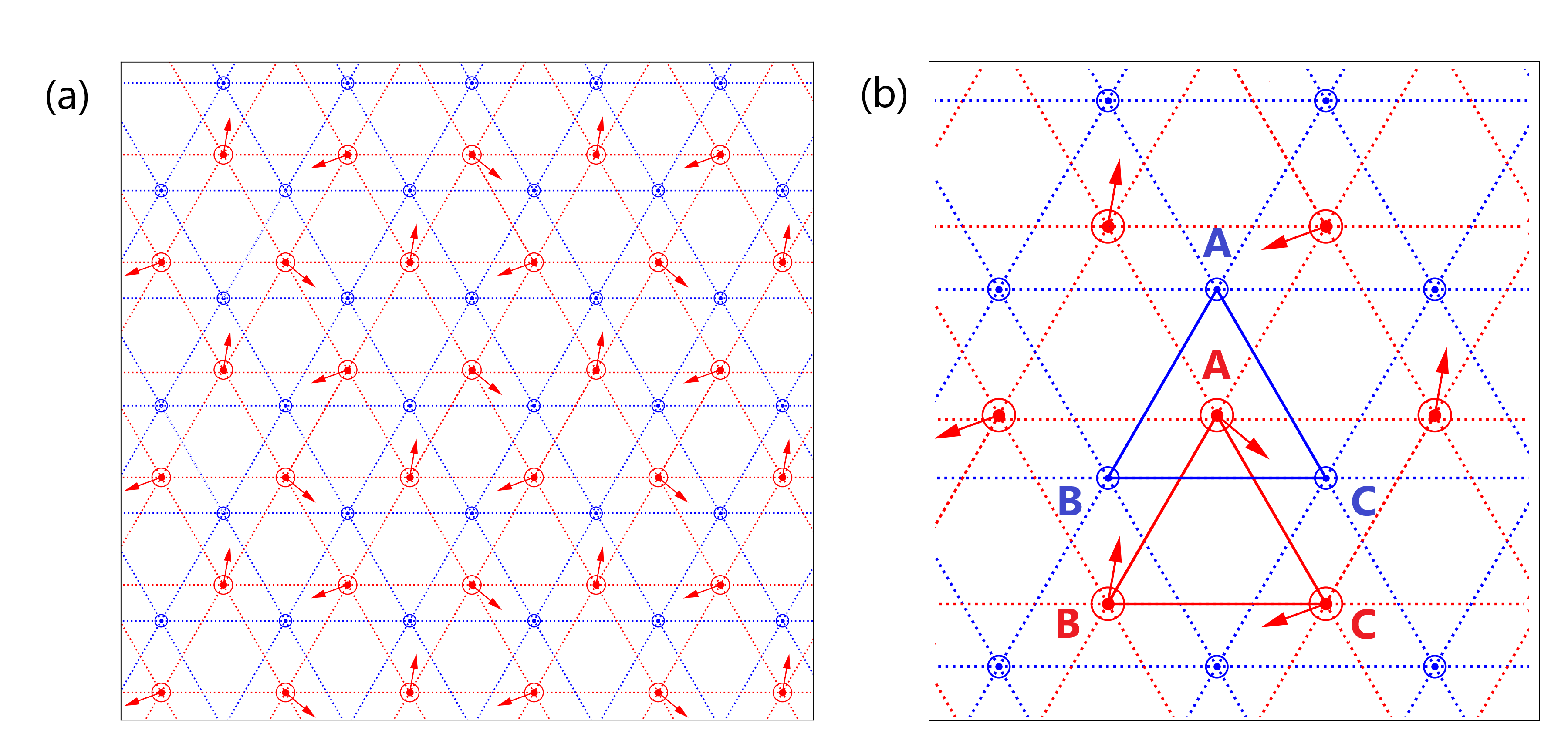
where () creates (annihilates) an electron at the Wannier orbital centered at the -th lattice site of sublattice with spin . Index distinguishes between two triangular sublattices consisting of the () and () stacking points in the MoTe2 and WSe2 layers, respectively (with and ). This results in a two-sublattice honeycomb structure [cf. Fig. 2(a)]. For () the summation over corresponds to the next-nearest-neighbor (nearest-neighbor) hopping at the honeycomb lattice. The intra- and inter-layer hoppings are complex and have the following form
| (3) |
| (4) |
where with () for () as well as () for () and for . Moreover, depending on the direction of the hopping while and increases counterclockwise when going around the MoTe2 lattice sites. The absolute values of the hopping amplitudes are set to =4.03 meV, =3.4 meV and =4 meV and have been taken from Ref. Rademaker, 2022.
It is worth emphasizing that this model includes same-spin interlayer hopping, which, by nature of the AB-stacking, implies also intervalley hoppping, as the spin-up valley in MoTe2 is at the opposite -point as the spin-up valley in WSe2. In a lowest order continuum model without interactions or lattice relaxation, such intervalley hopping would be vanishingly small. However, it has been argued that such hopping can arise through lattice relaxation,Zhao et al. (2022) or interaction effects.Dong and Zhang (2023) In this work we take the existence of interlayer/intervalley hopping as a starting point to study the effect of further interactions, without discussing the origin of such hopping.
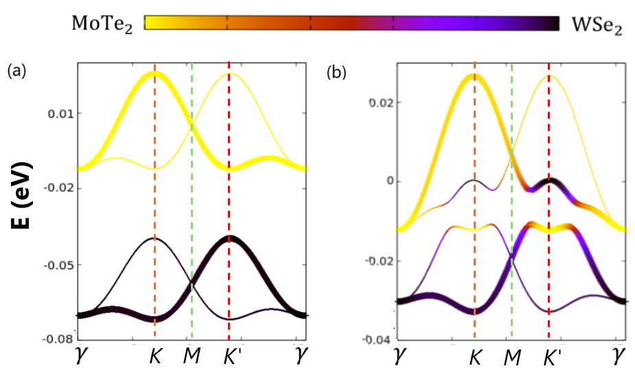
The last term of Eq. (2) represents the onsite contribution where , , meV, and introduces the effect of displacement field. For the top (bottom) band is composed only of the MoTe2 (WSe2) states while with increasing one pushes the bottom band to the upper which at some point initiates band inversion (cf. Fig. 1).
The second and the third terms in Eq. (1) introduce the onsite and intersite Coulomb repulsion and have the following form,
| (5) |
| (6) |
where determines the strength of the onsite repulsion while and correspond to the intra- and inter-layer Coulomb repulsion, respectively.
We implement the Hartree-Fock (HF) approximation for the interaction terms. The principal insights derived from our HF investigation are firmly validated by subsequent variational Gutzwiller approach, which we detail further below. After applying the HF treatment to the onsite interaction term given by Eq. (5), one obtains,
| (7) |
where, and . In the above equation we have introduced the following notation for the expectation values: and .
Application of the same approach to the intersite Coulomb repulsion given by Eq. (6) leads to,
| (8) |
where for and .
As one can see from Eq. (7), already at the level of such mean-field picture, the -term can lead to effective shift of the spin-up and spin-down onsite energies as well as to non-zero expectation values of the onsite spin rising and/or lowering operators. That points to a possible spin-ordered states that can be stabilized due to electron-electron interaction effects. In this study, we focus on the situation corresponding to one hole per moiré unit cell. In such case and for , one can project out the completely filled WSe2 band, which is separated by an energy gap from the half-filled MoTe2. That leads to an effective single-band model on a triangular lattice with nearest neighbor complex hoppingsRademaker (2022). It has been reported previously that in such situation the onsite Coulomb repulsion leads to a tendency towards an in-plane 120∘ antiferromagnetic alignmentBiborski et al. (2024). Additionally, for sufficiently high value of the single-band model can be transformed into a Heisenberg model supplemented with the Dzyaloshinskii-Moriya (DM) term which also points to a possible antiferromagnetic orderingPan et al. (2020). Based on those considerations, one should expect that for , also for the two band model considered here, the in-plane 120∘ AF alignment should appear at the MoTe2 layer [cf. Fig.2(a)]. Such ordered state can than evolve with increasing value of the displacement field. To allow for an initial AF alignment in our calculations we introduce a supercell containing 3 moiré unit cells, each consisting of one lattice site from the MoTe2 layer and one from the WSe2 layer [bold lines in Fig.2(b)]. Now, the expectation values of the occupation operator as well as the spin rising and lowering operators can vary within the supercell, but they need to repeat themselves when moving from one supercell to another. Namely, , , , where enumerates the supercells, determines the lattice site within the supercell with correspond to the two layers. In such notation the number of electrons per MoTe2 and WSe2 moiré orbitals is: and , respectively. Also, the total number of particles per lattice site takes the form . The relation between , and the components of the magnetization vectors are the following
| (9) |
As one can see, in principle, such approach allows for different orientations of the magnetization vector, , at each of the 6 lattice sites of the chosen supercell. In particular, the mentioned in-plane antiferromagnetic alignment at the MoTe2 layer can be realized, for which all the three vectors , for and , have equal module, no -component, and they form an angle of between each other.
In order to be able to effectively diagonalize the mean-field hamiltonian composed of Eqs. (2), (7) and (8), one can first carry out the transformation to the reciprocal space, which leads to
| (10) |
where is the number of supercells in the system and we have kept the scalar terms in the real-space representation. Also, we introduced a -dimensional composite creation and annihilation operators in -space defined by
| (11) |
and . Note that, the three moiré lattice sites per each layer are labeled by and , with distinctions between layers indicated by the respective layer indices, [cf. Fig. 2 (b)]. The matrix form of the Hamiltonian appearing in Eq. (10) is the following
| (14) |
As one can see, the resulting matrix is composed of two spin-conserving submatrices and two spin-mixing components, . The latter correspond to the onsite spin-flip operators and result from the onsite Coulomb repulsion. Those terms are responsible for the tendency towards in-plane 120∘ AF alignment. Each spin-conserving submatrices in Eq. (14) are defined as,
| (15) |
where takes the form
| (22) |
with and being the dependent inter- and intra-layer hopping contributions between the , , and lattice sites of both layers indicated by [cf. Eq. (2)]. All the onsite energies are now contained in the submatrices of the form
| (23) |
where
| (24) |
with being the chemical potential and , . Having the matrix form of our hamiltonian, one can diagonalize it and derive the self-consistent equations for all the mean-fields ( and ) as well as the chemical potential in a standard manner.
Since the system is characterized by significant Coulomb repulsion, the electron-electron correlations may play a role. To take that into account, apart from the HF approximation we additionally apply the Gutzwiller method which is based on the variational wave function of the form
| (25) |
where is the non-correlated state of the system and the correlation operator takes the form
| (26) |
with ’s being the variational parameters and being the states from the local basis (cf. Table 1).
| Combinations | ||
|---|---|---|
| 0 | ||
| 1 | ||
| 2 |
The parameters appearing in Eq. (26) can be cast in a matrix form
| (27) |
where we have assumed that the variational parameters do not depend on the index but only on the layer index () and the site index within the supercell (). Additionally, since we do not consider superconductivity here, we have set to zero the variational parameters corresponding to an onsite pairing terms. We consider Hermitian Gutzwiller operators [], thus the diagonal terms in Eq. (27) are real and . As shown in Ref. Bünemann et al., 1998 within such approach it is convenient to impose additional constraints to the correlation operator in order to eliminate the local contributions at the inner vertices which arise after the application of the Wick’s theorem. Namely,
| (28) |
| (29) |
where . After taking into account the above constraints, we are left with only one ’true’ variational parameter per lattice site. In our calculations we determine by minimizing the free energy of the system and all the remaining ’s are determined by using Eqs. (28) and (29).
In order to derive the expression for the energy expectation value we apply the so-called Gutzwiller approximation which is exact in the limit of infinite dimensions. The resulting formulas are the following
| (30) |
| (31) |
where = and
| (32) |
In the above Equation the diagonal and off-diagonal renormalization hopping factors have the form,
| (33) |
| (34) |
where () when (). For the calculations carried out with the use of the Gutzwiller approximation, we restrict ourselves to the situation with onsite interactions only, therefore, we do not provide the expectation value of the part of the Hamiltonian in the state.
As one can see from Eqs. (30) and (31), the expectation value of the original Hamiltonian in the correlated state can be expressed in terms of the expectation values in the non-correlated state. Therefore, one can construct an effective Hamiltonian so that within the Gutzwiller approximation. In such approach, hamiltonian can be treated within the mean field method with the correlation effects taken into account via the renormalization factors given by Eqs. (33), (34), and . Of course, in such approach the procedure of solving the self consistent equations has to be coupled with the minimization of the system energy over the variational parameters. It should be noted that here we are mainly focused on the situation with one hole per moiré lattice site, when the lower band is completely filled and the upper one is half-filled. In general it is expected that the renormalization is significant close to the half-filled situation. While moving away from half-filling the renormalization parameters are becoming close to one. Therefore, for the sake of simplicity, we only take into account the renormalization in the MoTe2 band.
The restricting conditions Eq. (28) and (29) are used to generate the necessary equations, which are solved numerically using a hybrid subroutine from the MINPACK library Devernay (2007), where is varied self-consistently in our calculations. It uses finite difference approximation of the Jacobian to estimate the Jacobian matrix when solving systems of nonlinear equations.
III Results
Within this Section we show the results of our calculations devided to two subsection. In subsection A we focus on the analysis of the topological and magnetic features of the system limiting to the onsite Coulomb repulsion only, whereas, the influence of the intersite repulsion as well the analysis of the charge ordered states is deferred to subsection B. For the sake of clarity while analyzing our results we replace the and indices which correspond to MoTe2 and WSe2 layers with and subscripts, respectively.
III.1 QAHI state formation
We first apply the Hartree-Fock approximation in order to analyze the formation of a non-trivial topological state within the Hubbard model of heterobilayer for one hole per moiré unit cell. At this filling, the QAHI behavior has been reported experimentally indicating the appearance of conductive edge states and an insulating bulk of the sampleDevakul and Fu (2022). In our analysis, we use the electron language, for which is equivalent to one hole per moiré unit cell and corresponds to completely filled lower band and half-filled upper band (cf. Fig. 1). For the sake of simplicity, we initially focus on the on-site Coulomb repulsion, taking , and introduce the following relation . Following the recent experimental reportZhao et al. (2023) we aim at reconstructing the band structure corresponding to a charge transfer insulator induced by substantial Hubbard . Hence, we set a relatively large value of , which is comparable to the one taken in Ref. Xie et al., 2024.
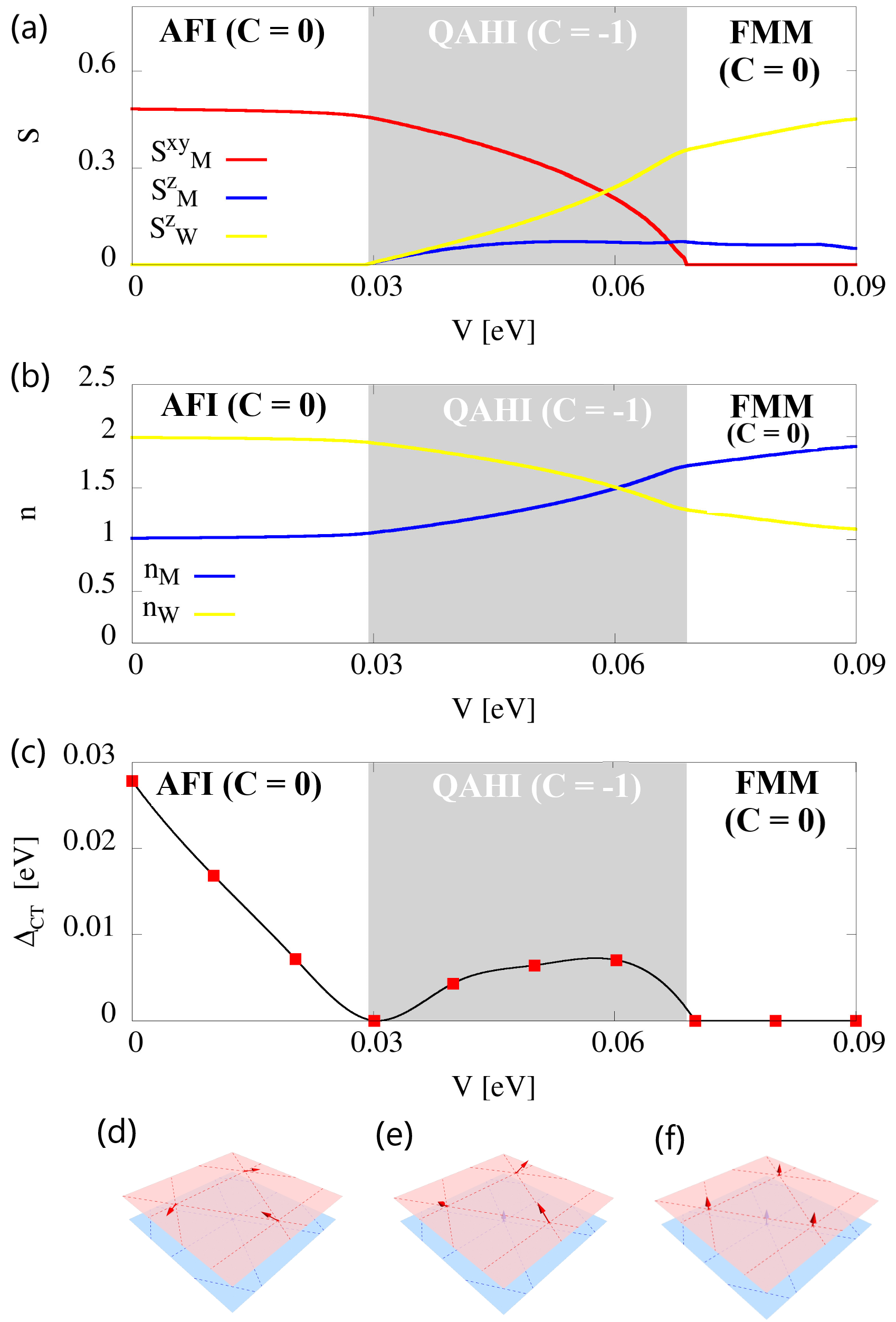
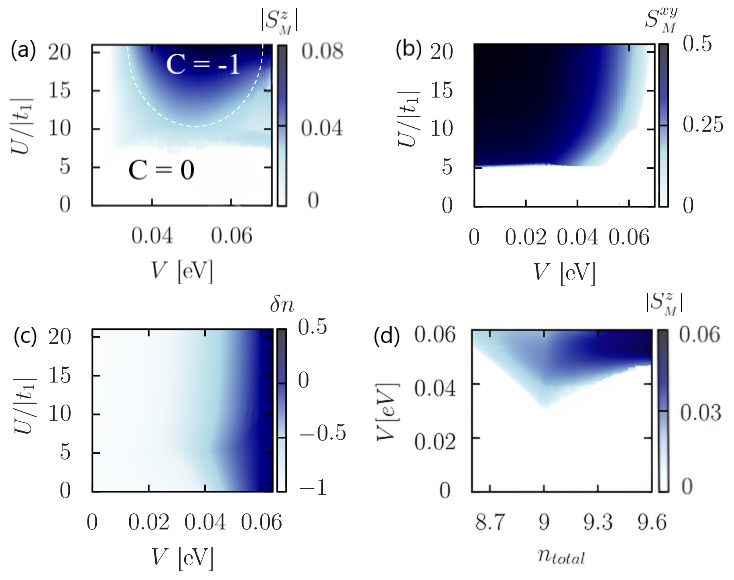
The calculated evolution of the magnetically ordered states with increasing displacement field is shown in Fig. 3(a). Initially, for small values of an in-plane 120∘ antiferromagnetic ordering is realized at the MoTe2 layer with the in-plane magnetization playing the role of the order parameter. No magnetic ordering appears at the WSe2 layer since its band is fully filled. At some critical value of the displacement field the out-of-plane magnetization in both layers become non-zero ( and ), leading to a superposition of in-plane AF ordering and out-of-plane FM ordering (canted AF order). According to our analysis this region corresponds to a Chern number indicating a quantum anomalous Hall insulating (QAHI) state. The details of the Chern number calculations together with the Berry curvature maps are provided in the Appendix. Finally, a second transition appears where the in-plane AF ordering is destroyed and only out-of-plane magnetization survives leading to a ferromagnetic metallic state (FMM). Additionally, in Fig. 3(b) we show the calculated number of electrons per MoTe2 and WSe2 moiré orbitals (, ). As one can see in the Figure, in the AFI state we start from the half-filled MoTe2 band () and completely filled WSe2 band (). After entering the QAHI region, due to band band mixing, the electrons are starting to be transferred from the WSe2 layer to the MoTe2 layer leading to a more homogeneous distribution of charge between the layers. However, close to the transition to the FMM state the situation becomes inverted. It should be noted that the appearance of canted 120∘ AF magnetic ordering with non-trivial topological features characterized by , has been reported quite recently and discussed in the context of MoTe2/WSe2 in Ref. Devakul and Fu, 2022.
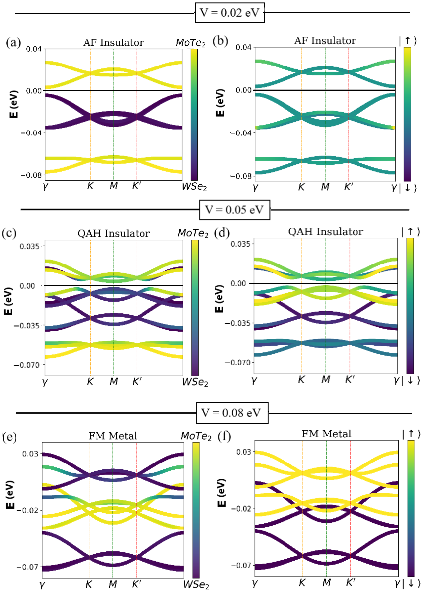
In order to gain some more insight in the origin of the obtained sequence of phases, in Fig. 4, we show the band structure for the three representative values of the displacement field corresponding to the three regimes seen in Fig. 3. The colored scale indicates the layer and spin state contribution in a given band. It should be noted that we plot the bands along the high symmetry points of the reduced mini Brillouin zone. The reduction is due to the introduction of the supercell which allows for the AF alignment in our calculations (cf. Sec. II). As one can see in the AFI state the upper MoTe2 band seen in Fig. 1 has spit into two subbands with the bottom one being located below the WSe2 band. For the upper MoTe2 subband is completely empty and separated by an energy gap from the fully occupied WSe2 band and the lower MoTe2 subband. Such band structure is consistent with the charge transfer insulating scenario. As the displacement field is increased the WSe2 band moves up, which from some point induces band mixing and emergence of the spin splitting due to the out-of-plane magnetization discussed earlier. In this state the gap is still open, but now the calculated Chern number of the upper MoTe2 subband is , which induces the QAHI behavior. It should be noted that due to the AF alignment in the QAHI state the spin lowering () and rising () expectation values are non-zero which together with the band mixing term allows for the realization of the valley coherent state indicated by the experimentsTao et al. (2024b) in which the hybridization of states from different layers and different valleys is allowed near the Fermi level. Nevertheless, for relatively large values of the displacement field the AF ordering is destroyed and the band splitting of the MoTe2 band disappears which results in gap closing and one is left with an out-of-plane FM metallic state. The two extreme situations of very low and very high displacement fields correspond to layer state separation [Fig. 4(a)] and spin state separation [Fig. 4(f)], respectively. In the intermediate region of QAHI, all states are mixed.
The results shown in Figs. 3 and 4 agree qualitatively with the available experimental data in the following aspects: (i) with increasing displacement field the system undergoes, first, a transition from the topologically trivial insulting to the QAH insulating state and than, a transition from the QAH to the metallic state appearsTao et al. (2024b); Li et al. (2021a); (ii) the QAH state possesses a spontaneous spin-polarization in both layers and the holes are distributed in both layersTao et al. (2024b); (iii) the QAH state realizes a valley-coherent state in which hybridization of states from different layers and different valleys is allowed near the Fermi levelTao et al. (2024b). One significant difference between our calculation and the experiment is the fact that we see a continuous gap-closing while approaching to the QAHI state, whereas in the experiments the gap seems to stay finite at the transitionLi et al. (2021a).
For the sake of completeness in Fig. 5 we show the in-plane and out-of-plane magnetization in the MoTe2 layer as functions of onsite Coulomb repulsion and displacement field. Since, the magnetically ordered states are induced spontaneously due to electron-interactions, some minimal value of is needed to stabilize them. One should note that the topologically nontrivial state on the -plane is obtained for the area in which both and [marked by the dashed white line in (a)]. As one can see, the range of displacement fields in which the QAHI state is stable, is getting narrower with decreasing . The minimal value for the appearance of QAHI is , where is the bare bandwidth of the upper band, which is in our case. Additionally, in (d) we show how the out-of-plane magnetization on the MoTe2 layer changes as one moves away from the half-filled situation. The results shown in (d) have been obtained for , which still leads to the appearance of the QAH but due to relatively smaller value of allows for better numerical convergence. One should note, that in this case only corresponds to an insulating state, since only than the fully occupied subbands/bands are separated by an energy gap from the fully empty subband (cf. Fig. 4).
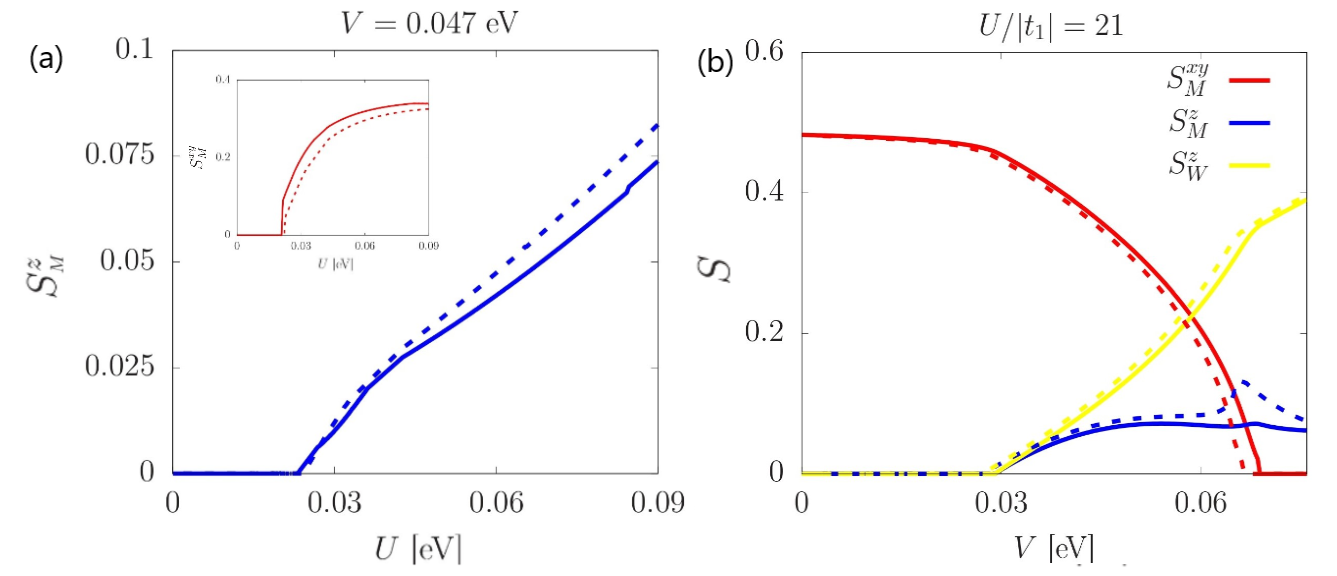
The comparison between the GA and HF methods is provided in Fig. 6. As one can see in the considered case both methods give similar results. It should be noted that within the Gutzwiller approximation the wave function is renormalized the most for the case of one electron per lattice site since in such case electron hopping leads to creation of double occupancy which in turn corresponds to significant increase of system energy due to strong onsite Coulomb repulsion. For a single band model half-filling always corresponds to such scenario. However, in a two band model analyzed here, where band mixing appears, even for half-filling of the upper band (), the electrons can be distributed in the layers in such case that and (cf. fig. 3). That diminishes the the effect of the correlation operator most probably leading to similarities between the HF and GA calculations. Also, for when the band mixing is absent we are dealing with nearly saturated 120∘ AF state and again both in GA and HF are close.
III.2 Influence of the intersite Coulomb repulsion
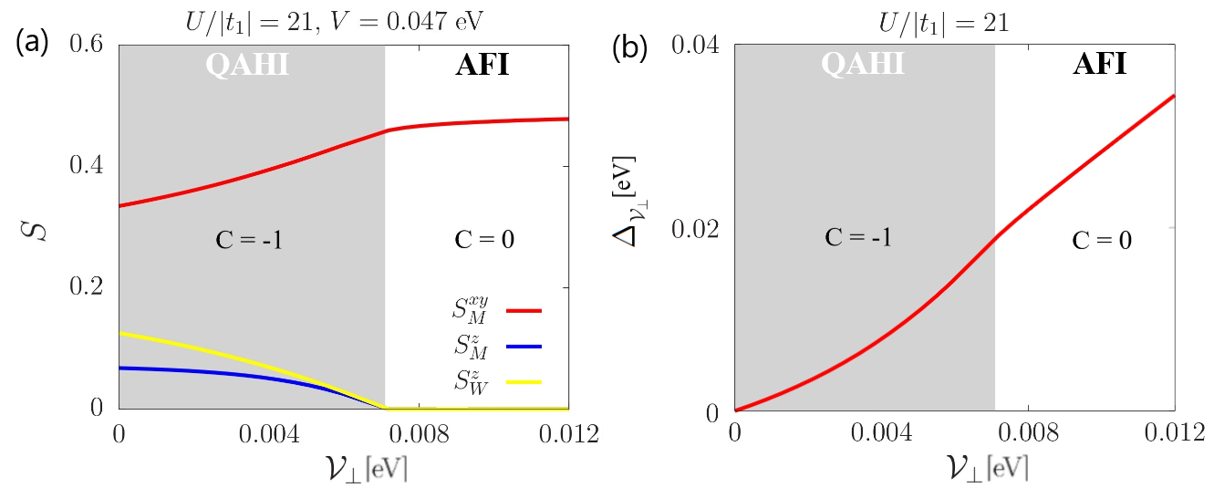
Here we analyze the influence of the intersite Coulomb repulsion terms. We first set the displacement field to the value of meV, which corresponds to the stability of the QAHI, and analyze the evolution of this state with increasing interlayer Coulomb term . In Fig. 7 we show the -dependence of both in-plane and out-of-plane magnetizations together with the value of the Chern number corresponding to particular considered regimes. It should be noted that within the HF approach, the -term leads to an effective onsite energies at the two layers [cf. Eq. (8)]. The difference between the MoTe2 and WSe2 onsite energies resulting from the considered effect is shown in Fig. 7(b) and can be expressed in the following manner
| (35) |
With increasing one actually increases the charge transfer gap between the upper MoTe2 subband and the WSe2 band (cf. Fig. 4). Such effect is equivalent to decreasing the displacement field shown in the previous part of our analysis (cf. Fig. 3). Consequently, by enhancing one eventually can destroy the QAHI state by suppressing the band mixing.
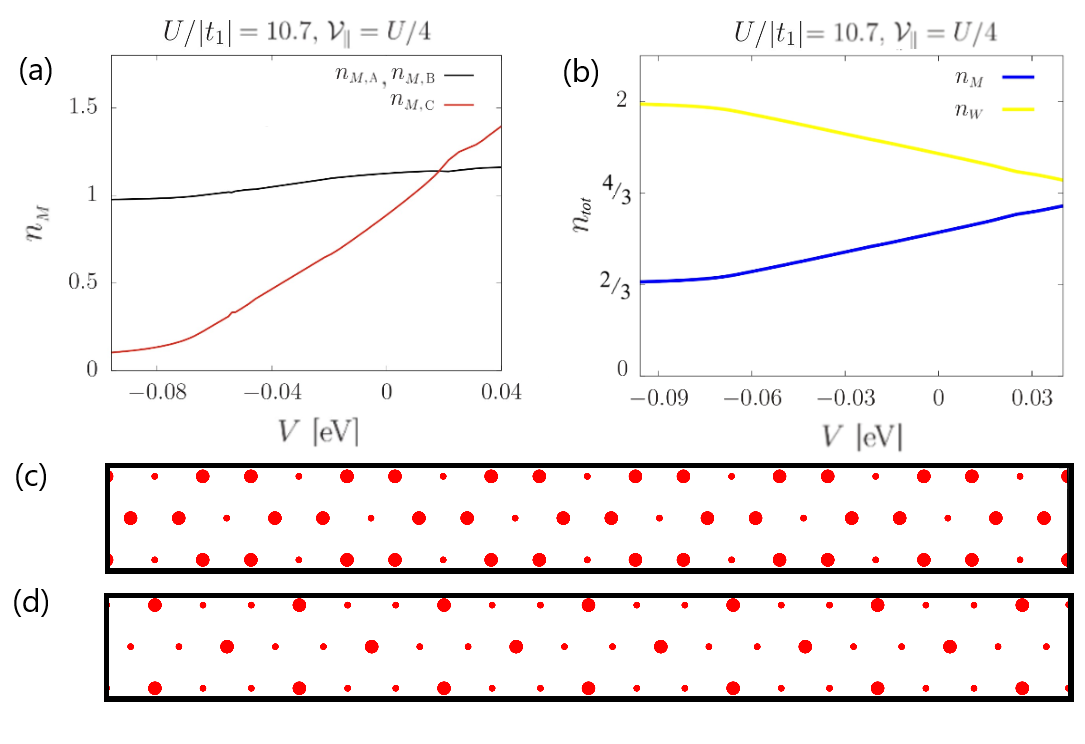
Next we include the intralayer intersite Coulomb repulsion and focus on the scenario of in order to study the formation of the charge ordered phase. In this part of the analysis, we have decreased the value of onsite Coulomb repulsion to which leads to relatively better convergence of the numerical procedure. Following Ref. Xie et al., 2024 we set and initially consider a relatively large negative bias voltage to separate significantly the MoTe2 and WSe2 bands leading to a fractional filling of and , as shown in Fig. 8 (b). In Fig. 8(a) we show the average number of particles on the three lattice sites () of the MoTe2 layer (cf. Fig. 2) as functions of the displacement field. As one can see for large negative , the lattice site of the MoTe2 layer becomes nearly vacant, with two remaining sites ( and ) being singly occupied. Such charge distribution minimizes the interaction energy resulting from the -term.
Similarly as before, by increasing the displacement field we change the distribution of carriers among the two layers [cf. Fig. 8(b)]. As shown in Fig. 8(a), this weakens the amplitude of the charge modulation since with increasing we are moving away from the fractional filling of . Consequently, at some point the situation becomes inverted, meaning that a transition appears from a honeycomb structure of increased carrier concentration, shown in Fig. 8(c), to a honeycomb structure of decreased carrier concentration shown as in Fig. 8(d).
It should be noted that different forms of charge ordered states have been experimentally evidenced in TMD based moiré systems at fractional fillingsRegan et al. (2020); Li et al. (2021b, c, 2024). In particular in WSe2/WS2, a honeycomb charge pattern, similar to the one analyzed here, has been imaged by using a non-invasive STM spectroscopy techniqueLi et al. (2021b). It should be noted that the WSe2/WS2 system should correspond a very similar single particle model as the one considered here for the case of the MoTe2/WSe2 as shown in Ref. Rademaker, 2022.
IV Conclusions
We applied the effective two-band moiré Hubbard model to analyze the interplay between electron-electron interactions and the topological features of MoTe2/WSe2 heterobilayer. According to our calculations, at half filling () and for large enough values of the onsite Coulomb repulsion the upper MoTe2 band splits into two subbands creating an in-plane 120∘ AF charge transfer insulator. However, by increasing the displacement field one decreases the charge transfer gap leading to band inversion as well as the appearance of an out-of-plane magnetization. These two effects result in a formation of charge transfer QAH insulating state. By a further increase of the displacement field, one suppresses the in-plane AF insulating state leading to a out-of-plane FM metallic state. Such sequence of phases agrees qualitatively with the available experimental data Li et al. (2021a); Tao et al. (2024b). Another aspect which is seen both here and in the experiments is that the QAHI state possesses a spontaneous spin-polarization in both layers and the holes are distributed in both layersTao et al. (2024b).
It should be noted that recent layer- and helicity-resolved optical spectroscopy measurements suggest that the QAH state correspond to a valley-coherent scenario, in which the hybridization of states from different layers and different valleys is allowed near the Fermi levelTao et al. (2024b). In our case, as we show in Fig. 3, the two limiting situations of very small and very large displacement fields correspond to no-layer mixing (but spin mixing allowed) and no-spin mixing (but layer mixing allowed), respectively. The QAH state correspond to an intermediate region between the two, leading to both spin and layer mixing. Such situation is in agreement with the mentioned valley-coherent state indicated by the experiments.
Additionally, we have analyzed the influence of the inter-site Coulomb repulsion terms. In particular, as we show the intersite interlayer Coulomb term () leads to a similar effect as the one induced by decreasing the displacement field. As such it might have a destructive influence on the QAHI state. Such effect can be understood in terms of effective onsite energies tuned by the after the Hartree-Fock decomposition. Namely by increasing one increases the charge transfer gap removing the band inversion which is crucial for the QAHI state formation.
After the inclusion of the intersite intralayer Coulomb repulsion term (), we have considered the fractional filling of the upper band, in order to analyze the possibility of charge ordering. According to our calculations the charge density wave state realizing a pattern of honeycomb lattice sites of increased electron concentration at the MoTe2 layer, is realized in the regime of low displacement fields. However, since by displacement field one changes the distribution of charge between the layers the CDW amplitude is decreased with increasing . At some point a inverse situation of a pattern of honeycomb lattice sites of decreased electron concentration at the MoTe2 layer appears.
For the sake of completeness we have also supplemented our Hartree-Fock result with those stemming from the Gutzwiller approximation method. According to this part of the analysis the changes seems to be quantitative with stronger tendency towards magnetic ordering appearing for the GA solution. However, from the qualitative point of view both methods lead to similar physical picture of the considered model .
The code which was written to carry out the numerical calculations as well as the data behind the figures are available in the open repositoryZegrodnik (2024).
Acknowledgements.
This research was partly supported by National Science Centre, Poland (NCN) according to Decision No. 2021/42/E/ST3/00128 and partly by program “Excellence initiative–research university” for the AGH University of Krakow. For the purpose of Open Access, the author has applied a CC-BY public copyright licence to any Author Accepted Manuscript (AAM) version arising from this submission.Appendix A Second Chern Number
Here, we present a comprehensive numerical methodology which has been applied here to accurately compute the second Chern number characterizing the considered system. Note, that due to introduction of the supercell consisting of six moiré orbitals (cf. Fig. 2), the resulting band structure consists of nine dispersion relation branches in the folded mini Brillouin zone (cf. Fig. 4). For the upper three branches correspond to empty states, which in the QAHI state are separated by a band gap from the occupied bands. In order to calculate the Chern number effectively one can focus on those three dispersion relation branches collectively. This approach leverages some basics of numerical approximations in lattice gauge theory. Instead of a single state, we will consider a subspace spanned by a set of three degenerate states () with the same quantum number .
For the adiabatic evolution of a quantum state, the superimposed state is obtained from a unitary transformation of the original states,
| (36) |
This is the U(3) gauge transformation applied to describe transformation properties of gauge potential and quantum state during it’s evolution. With the time dependence of the parameter space, a dynamical phase factor is simply multiplied with the final state,
| (37) |
where, the unitary matrix Wilczek and Zee (1984) contains all the connection terms along a closed contour given by,
| (38) |
The path ordering is crucial so that the non-Abellian gauge potential can remain non-commutative, thus following the properties of a matrix with each element given by,
| (39) |
Such unitary transformation rule is operative in continuous parameter or -space. To recover the discrete formula, we use the method used by Fukui-Hatsugai-Suzuki Fukui et al. (2005). We need to define a U(1) link variable for parallel transport between any two neighboring points and in the base manifold,
| (40) |
where, and is the normalization constant.
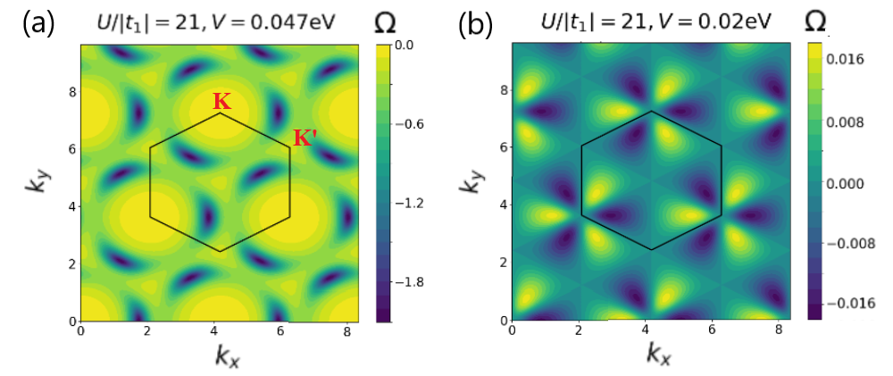
In Fig. 9 we show the calculated Berry curvature maps in momentum space for two selected values of the displacement field eV and eV, corresponding to the (QAHI) and (AFI), respectively.
In this numerical calculation, we broke the entire Brillouin zone into small rectangular plaques and calculated the winding number for each of them which is given by,
| (41) |
Consequently, the above equation can be written in terms of the link variables by applying the periodic gauge potential,
| (42) |
By carefully evaluating each -point across the entire Brillouin zone, we arrive at the final result presented below,
| (43) |
where, . We can write the compact form of the above term by summing up not all the points but all the small plaques,
| (44) |
where, represents the determinant of product of the four link variables.
Using Eq. (44), the non-Abelian Berry curvature in -space is identified as the phase, divided by the area of each small plaque . When is on the higher side, the phase diagram for the top three moiré bands can be obtained by carefully comparing the results.
References
- Ghiotto et al. (2021) A. Ghiotto, E.-M. Shih, G. S. S. G. Pereira, D. A. Rhodes, J. Kim, Bumho Zang, A. J. Millis, K. Watanabe, T. Taniguchi, J. C. Hone, L. Wang, C. R. Dean, and A. N. Pasupathy, Nature 597, 345 (2021).
- Wang et al. (2020) L. Wang, E.-M. Shih, A. Ghiotto, L. Xian, D. A. Rhodes, C. Tan, M. Claassen, D. M. Kennes, Y. Bai, B. Kim, K. Watanabe, T. Taniguchi, X. Zhu, J. Hone, A. Rubio, and C. R. Pasupathy, Abhay N. amd Dean, Nature Materials 19, 861 (2020).
- Zhao et al. (2023) W. Zhao, B. Shen, Z. Tao, Z. Han, K. Kang, K. Watanabe, T. Taniguchi, K. Mak, Fai, and J. Shan, Nature 616, 61 (2023).
- Li et al. (2021a) T. Li, S. Jiang, B. Shen, Y. Zhang, L. Li, Z. Tao, T. Devakul, K. Watanabe, T. Taniguchi, L. Fu, J. Shan, and K. F. Mak, Nature 600, 641–646 (2021a).
- Tao et al. (2024a) Z. Tao, B. Shen, S. Jiang, T. Li, L. Li, L. Ma, W. Zhao, J. Hu, K. Pistunova, K. Watanabe, T. Taniguchi, T. F. Heinz, K. F. Mak, and J. Shan, Phys. Rev. X 14, 011004 (2024a).
- Tao et al. (2024b) Z. Tao, B. Shen, W. Zhao, C. Hu, Nai, T. Li, S. Jiang, L. Li, K. Watanabe, T. Taniguchi, A. H. MacDonald, J. Shan, and F. Mak, Kin, Nature 19, 28 (2024b).
- Rademaker (2022) L. Rademaker, Phys. Rev. B 105, 195428 (2022).
- Devakul and Fu (2022) T. Devakul and L. Fu, Phys. Rev. X 12, 021031 (2022).
- Zhao et al. (2022) W. Zhao, K. Kang, Y. Zhang, P. Knüppel, Z. Tao, L. Li, C. L. Tschirhart, E. Redekop, K. Watanabe, T. Taniguchi, A. F. Young, J. Shan, and K. F. Mak, Nature Physics , 1 (2022).
- Guerci et al. (2023) D. Guerci, J. Wang, J. Zang, J. Cano, J. H. Pixley, and A. Millis, Science Advances 9, eade7701 (2023).
- Xie et al. (2024) F. Xie, L. Chen, and Q. Si, Phys. Rev. Res. 6, 013219 (2024).
- Dong and Zhang (2023) Z. Dong and Y.-H. Zhang, Phys. Rev. B 107, L081101 (2023).
- Pan et al. (2022) H. Pan, M. Xie, F. Wu, and S. Das Sarma, Phys. Rev. Lett. 129, 056804 (2022).
- Chang and Chang (2022) Y.-W. Chang and Y.-C. Chang, Phys. Rev. B 106, 245412 (2022).
- Biborski et al. (2024) A. Biborski, P. Wójcik, and M. Zegrodnik, Phys. Rev. B 109, 125144 (2024).
- Pan et al. (2020) H. Pan, F. Wu, and S. Das Sarma, Phys. Rev. Res. 2, 033087 (2020).
- Bünemann et al. (1998) J. Bünemann, W. Weber, and F. Gebhard, Phys. Rev. B 57, 6896 (1998).
- Devernay (2007) F. Devernay, “C/c++ minpack,” http://devernay.github.io/cminpack (2007).
- Regan et al. (2020) E. C. Regan, D. Wang, C. Jin, M. I. Bakti Utama, B. Gao, X. Wei, S. Zhao, W. Zhao, Z. Zhang, K. Yumigeta, M. Blei, J. D. Carlström, K. Watanabe, T. Taniguchi, S. Tongay, M. Crommie, A. Zettl, and F. Wang, Nature 579, 359 (2020).
- Li et al. (2021b) H. Li, S. Li, E. C. Regan, D. Wang, W. Zhao, S. Kahn, K. Yumigeta, M. Blei, T. Taniguchi, K. Watanabe, S. Tongay, A. Zettl, M. F. Crommie, and F. Wang, Nature 597, 650 (2021b).
- Li et al. (2021c) T. Li, J. Zhu, Y. Tang, K. Watanabe, T. Taniguchi, V. Elser, J. Shan, and K. F. Mak, Nature 16, 1068 (2021c).
- Li et al. (2024) H. Li, Z. Xiang, A. P. Reddy, T. Devakul, R. Sailus, R. Banerjee, T. Taniguchi, K. Watanabe, S. Tongay, A. Zettl, L. Fu, M. F. Crommie, and F. Wang, Science 385, 86 (2024).
- Zegrodnik (2024) M. Zegrodnik, “Quantum anomalous hall state in mote2/wse2 heterobilayer [data set]. zenodo. https://doi.org/10.5281/zenodo.14410816,” (2024).
- Wilczek and Zee (1984) F. Wilczek and A. Zee, Phys. Rev. Lett. 52, 2111 (1984).
- Fukui et al. (2005) T. Fukui, Y. Hatsugai, and H. Suzuki, Journal of the Physical Society of Japan 74, 1674 (2005).