High-energy Coulomb scattering of spatially extended particles

Abstract

We analyze pure Coulomb high-energy elastic scattering of charged particles (hadrons or nuclei), discarding their strong interactions. We distinguish three scattering modes, determined by the magnitude of the momentum transfer, in which particles behave as point-like, structureless extended, and structured composite objects. The results are compared in the potential and QFT approaches of the eikonal model.

1 Introduction

At low momentum transfer the Coulomb and strong interactions make compete contributions to the elastic scattering of charged particless. In this regard, the determination of Coulomb contributions and then the description of Coulomb-nuclear interference (CNI) is an essential part of the study of strong interactions of hadrons in the small-transfer region. Meanwhile, despite the impressive history of the issue [1]-[11] the problem of the Coulomb contributions has not yet been completely solved. In particular, there is no consensus on how to account for the spatial sizes of charged particles, such as protons. Similar problems arise when describing the Coulomb scattering of heavy nuclei with large electric charges on each other.

At high energies, the generally accepted method for describing Coulomb scattering is based on the eikonal model, which ensures the summation of Coulomb contributions in scattering at small angles. However, in different versions of this model, the eikonal phase is defined differently. Most studies use the potential version, see e.g. [4]-[10] and references therein, in which the eikonal phase, as well as the Born contribution, are determined through the classical potential interaction of electric charges. In the quantum field theory (QFT) version of the model, the eikonal phase and the Born contribution are determined by the simplest diagram with the one-photon exchange in the $t$-channel, see e.g. [12, 13]. In the case of point-like particles the mentioned difference is ultimately unimportant. However, in the case of spatially extended particles it leads to different prescriptions for taking into account the electromagnetic form factors. Namely, in the potential approach, particle form factors directly enter the eikonal phase, while in the QFT form factors arise when averaging the full amplitude operator between the wave functions of in- and out-states, and therefore appear as factors in the full amplitude.

In fact, both above approaches are based on the idea of particles as extended structureless objects. However, the mode of multiple Coulomb scattering on their structural components is also possible. We mean the scattering on charged partons in the case of hadrons and on charged protons in the case of scattering of nuclei. In both cases, each act of elementary scattering must contribute to the Born amplitude. Such a scattering mode was described by Glauber [14] in relation to elastic scattering due to strong interactions of a fast point-like particle off a nucleus. Subsequently, many attempts were made to generalize this approach to the case of nucleus-nucleus scattering, each time using the short-range property of nuclear forces, see e.g. [15]-[20]. However, the generalization that is important for heavy nuclei to the case of scattering due to long-range Coulomb forces has not yet been consistently obtained. Accordingly, there is no generalization to the case of Coulomb scattering of hadrons on charged partons.

In this article, we explore the above issues and determine which scattering mode actually occurs and under what conditions. The key point will be the idea that the scattering mode is determined by the magnitude of the momentum transfer. In particular, at the very small transfers ($q^{2}\lesssim 10^{-2}\,\mbox{GeV}^{2}$ in the case of protons) the wavelength of the exchanged photons is of the order or exceeds the transverse sizes of colliding particles. In this case they scatter as structureless objects. At higher transfers, the scattering can occur on the charged components of the particles. In the latter case, the scattering must be described by the Glauber theory. We consistently construct its generalization to the case of Coulomb scattering of composite objects and show that the so-called optical approximation is indeed the leading one if the scattering objects contain a large number of charged components.

In the next section we discuss Coulomb scattering of point-like particles. The generalization to the case of extended particles in different scattering modes is given in Sect. 3. There we also carry out numerical simulations with different methods of accounting form factors. In the final section we discuss the results.

2 Coulomb scattering of point-like particles

Following the notation of [5, 11], we define the amplitude of elastic scattering of point-like particles at high energies in the eikonal approach as follows:

$$F(s,q^{2})=\frac{s}{4\pi\mbox{i}}\int\mbox{d}^{2}{\bf b}\;\;e^{\mbox{\scriptsize{i}}{\bf qb}}\left[e^{2\mbox{\scriptsize{i}}\delta(s,{\bf b})}-1\right].$$ (1)

Here $s$ is the square of the energy of colliding particles in the center-of-mass system, ${\bf q}$ is the momentum trasfer, $q^{2}={\bf q}^{2}=-t$, ${\bf b}$ is the impact parameter, $\delta(s,{\bf b})$ is the phase shift. From here on, two-dimensional vectors in the plane of impact parameter are denoted in bold without an arrow at the top. Amplitude (1) corresponds to the definition of the differential cross section as

$$\frac{\mbox{d}\sigma}{\mbox{d}t}=\frac{\pi}{sp^{2}_{cm}}|F|^{2}\,,$$ (2)

where $p^{2}_{cm}=s/4$. Expression (1) is a consequence of the well-known formula for the expansion of the amplitude in partial waves at large momenta and small scattering angles. Up to this limitation, formula (1) is model-free.

A specific model is determined by the phase shift $\delta(s,{\bf b})$. In the potential approach, it is determined by the interaction potential of particles [14, 21],

$$\delta(s,{\bf b})=-\,\frac{1}{2}\,\int_{-\infty}^{+\infty}\mbox{d}z\;V(s,\vec{\bf r})\,.$$ (3)

Hereinafter $\vec{\bf r}=({\bf b},z)$, where $z$ is the longitudinal coordinate. The potential $V(s,\vec{\bf r})$ simultaneously defines the Born amplitude,

$$F_{\mbox{\scriptsize Born}}(s,{\bf q}^{2})=-\frac{s}{4\pi}\,\int\mbox{d}^{3}\vec{\bf r}\;e^{\mbox{\scriptsize{i}}\vec{\bf q}\vec{\bf r}}\;V(s,\vec{\bf r}){\bigl{|}_{q_{z}=0}\bigr{.}}\,.$$ (4)

So $\delta(s,{\bf b})$ may be written as

$$\delta(s,{\bf b})=\frac{2\pi}{s}\int\frac{\mbox{d}^{2}{\bf q}}{(2\pi)^{2}}\;e^{-\mbox{\scriptsize{i}}{\bf qb}}F_{\mbox{\scriptsize Born}}(s,{\bf q}^{2})\,.$$ (5)

It should be noted here that the derivation of formula (3) is based on the non-relativistic Schrödinger equation. This implies that the total energy of the system is divided into potential and kinetic parts, and the kinetic energy of the scattering particles is determined, in particular, in the center-of-mass system by the non-relativistic formula $E_{kin}=p^{2}_{cm}/2m$, where $m$ is the reduced mass. We emphasize that the latter condition is essential for deriving formula (3). For this reason, extending the scope of application of this formula to the case of relativistic scattering is, at least, a strong model assumption. Fortunately, the final formulas for the amplitude turn out to be (formally) relativistically invariant. A posteriori, this justifies the use of this approach, but only until another, more suitable approach appears. (We will return to discuss this issue below.)

In QFT models, of course, there are no problems with relativistic invariance. In this case the phase shift $\delta(s,{\bf b})$ is determined directly by formula (5), where $F_{\mbox{\scriptsize Born}}$ is the simplest contribution to the amplitude due to the exchange in the $t$-channel by the appropriate particle acting as a quantum of interaction. Formula (1) in this case describes the result of summing a generalized ladder of similar exchanges in the approximation of large $s$ and restricted $t$ [12, 13].

In the specific case of Coulomb interaction, if we assume that the potential for point-like particles is $V^{C}(\vec{\bf r})=\alpha/|\vec{\bf r}|$, where $\alpha$ is the fine-structure constant, then the corresponding Born amplitude according to (4) is

$$F^{C}_{\mbox{\scriptsize Born}}=-\frac{\alpha s}{{\bf q}^{2}+\lambda^{2}}\,.$$ (6)

Here $\lambda$ is a parameter introduced to regularize IR divergences, which should eventually be directed to zero. In the QFT approach, the Coulomb Born amplitude is described by the same formula (6). So, in the case of point-like particles, the formulations of the eikonal model for Coulomb scattering in the potential and QFT approaches completely coincide.

Substituting (6) into (5), we get the phase shift

$$\delta^{C}({\bf b})=\frac{1}{2\pi}\int\mbox{d}^{2}{\bf q}\;e^{-\mbox{\scriptsize{i}}{\bf qb}}\frac{-\alpha}{q^{2}+\lambda^{2}}=-\alpha\mbox{K}_{0}(b\lambda)\,,$$ (7)

where $\mbox{K}_{0}(z)$ is the McDonald function of the zero order. Substituting (7) into formula (1), we obtain (see details in [11]) the following result:

$$F^{C}(s,q^{2}){\bigl{|}_{\lambda\to 0}\bigr{.}}=-\,\frac{s\alpha}{q^{2}}\,e^{\mbox{\scriptsize{i}}\alpha\ln(\lambda^{2}/q^{2})}e^{\mbox{\scriptsize{i}}\Phi(\alpha)}+\mbox{i}s\pi\delta({\bf q})\,.$$ (8)

Here $\delta({\bf q})$ is the delta-function and $\Phi(\alpha)=2\alpha\gamma-\mbox{i}\ln\left\{\Gamma(1+\mbox{i}\alpha)/\Gamma(1-\mbox{i}\alpha)\right\}$ is a real value. Correspondingly, $[\mbox{i}\alpha\ln(\lambda^{2}/q^{2})+\mbox{i}\Phi(\alpha)]$ determines a phase that accumulates IR-divergent contributions in accordance with general theorems on the elimination of IR divergences. The emergence of the phase is a consequence of the summation of the generalized ladder of Born contributions. For ${\bf q}\not=0$ the phase does not contribute to the cross section and can be omitted along with the $\delta$-function.

3 Spatially extended particles

The formalism considered above is quite applicable for describing scattering of extended charged particles in the case of extremely small values of transferred momenta, when the wavelengths of the exchanged photons significantly exceed the transverse sizes of colliding particles. As the transfer increases and the wavelengths of photons become comparable to the particle sizes, their sizes must be taken into account. In particular, if the wavelength of a photon exceeds but is comparable to the sizes of the particles, then the time of emission and absorption of the photon exceeds the time of interaction between internal parts of the particles. As a result, the scattering occurs immediately on all of their charged parts, and the photon exchange occurs between the volumes of particles without reference to specific points of emission and absorption. (In essence, these points are of a probabilistic nature.) Colliding particles in this case look like structureless objects equipped with a continuous charge distribution density. With a further increase in $q^{2}$, when the wavelength of photons becomes smaller than the distance between centers of charged components of the particles, Coulomb scattering should increasingly occur on these components. In the case of nuclei such charged components are protons, and in the case of hadrons they are charged partons.

Both the above modes can be analyzed in the potential and QFT approaches, and the results, generally speaking, may not coincide. In case of discrepancy, its cause should be understood. Below we begin to analyse this issue, starting with the scattering mode in which particles behave as structureless extended objects. In the case of protons, this mode occurs at $q^{2}\lesssim 10^{-2}\,\mbox{GeV}^{2}$, which roughly corresponds to distances of two or more of their radii. (In the same range of the transfer CNI effect is significant at the LHC energies [22, 23, 24].) In the case of nuclei, for example Pb-Pb Coulomb scattering, a similar estimate is $q^{2}\lesssim 2\times 10^{-4}\,\mbox{GeV}^{2}$. The cases with higher momentum transfers, we consider in further subsections.

3.1 Particles with continuous charge distribution

In the potential approach, a generally accepted way to generalize eikonal model to the case of scattering of extended particles is to introduce form factors in the eikonal phase. Actually, such a generalization should follow from the appropriate modification of the definition of potential in formula (3). Below we show this in the case when scattering particles are structureless objects characterized by a continuous charge distribution.

In doing so, we will pay special attention to issues of relativistic invariance. Namely, we will give a consistent derivation of the formula for the Coulomb shift proceeding from formula (3), based on the laws of classical electrodynamics. In particular, we will take into account the phenomenon of potential retardation in reference frames where both particles are moving.

So, let particles $a$ and $b$, each with electric charge $\sqrt{\alpha}$, are characterized by charge distribution densities $\mbox{\eulerRM\char 26\relax}_{\kappa}(\vec{\bf r}_{\kappa})$, $\kappa=a,b$. In this case $\mbox{d}q_{\kappa}=\sqrt{\alpha}\,\mbox{d}\vec{\bf r}_{\kappa}\mbox{\eulerRM\char 26\relax}_{\kappa}(\vec{\bf r}_{\kappa})$ is the elementary electric charge located in the spatial volume $\mbox{d}\vec{\bf r}_{\kappa}$, and in any reference frame the charge distribution density $\mbox{\eulerRM\char 26\relax}_{\kappa}(\vec{\bf r}_{\kappa})$ is normalized by the condition

$$\int\mbox{d}\vec{\bf r}_{\kappa}\mbox{\eulerRM\char 26\relax}_{\kappa}(\vec{\bf r}_{\kappa})=1\,.$$ (9)

First, we consider the rest frame of particle $a$. In this case, the elementary charge $\mbox{d}q_{a}$ forms a static electric potential $\mbox{d}\phi_{a}(\vec{\bf r})=\mbox{d}q_{a}/|\vec{\bf r}|$, where $\vec{\bf r}$ specifies a point in space relative to the location $\mbox{d}q_{a}$. Now let particle $b$ move in the direction of particle $a$ along the $z$ axis with impact parameter ${\bf b}$. If an elementary charge $\mbox{d}q_{b}$ appears in the point $\vec{\bf r}$, then the potential energy of interaction of these elementary charges is $\delta V^{C}_{ab}(\vec{\bf r})=\mbox{d}q_{a}\mbox{d}q_{b}/|\vec{\bf r}|$. Hence, the potential energy of interaction of particles $a$ and $b$ in this reference frame is

$$V^{C}_{ab}(\vec{\bf r})=\int\mbox{d}\vec{\bf r}_{a}\mbox{\eulerRM\char 26\relax}_{a}(\vec{\bf r}_{a})\,\mbox{d}\vec{\bf r}_{b}\mbox{\eulerRM\char 26\relax}_{b}(\vec{\bf r}_{b})\,\frac{\alpha}{|\vec{\bf r}-\vec{\bf r}_{a}+\vec{\bf r}_{b}|}\,,$$ (10)

where $\vec{\bf r}$ determines the position of the center of particle $b$ relative to the center of particle $a$, $\vec{\bf r}_{a}$ and $\vec{\bf r}_{b}$ are the radius-vectors of elementary charges relative to the centers of the corresponding particles. Next, we put $\vec{\bf r}=({\bf b},z)$, $\vec{\bf r}_{a}=({\bf s}_{a},z_{a})$, $\vec{\bf r}_{b}=({\bf s}_{b},z_{b})$, substitute (10) into (3) assuming that the latter formula is valid in the rest frame of particle $a$, and integrate first over $\mbox{d}z$. Then we obtain a formula for the Coulomb shift in the case of spatially extended particles,

$$\delta^{C}_{ab}({\bf b})=\int\mbox{d}{\bf s}_{a}\mbox{d}{\bf s}_{b}\,\rho_{a}({\bf s}_{a})\rho_{b}({\bf s}_{b})\,\delta^{C}({\bf b}-{\bf s}_{a}+{\bf s}_{b})\,.$$ (11)

Here $\rho_{a}({\bf s}_{a})$ and $\rho_{b}({\bf s}_{b})$ are the result of integration $\mbox{\eulerRM\char 26\relax}_{a}(\vec{\bf r}_{a})$ and $\mbox{\eulerRM\char 26\relax}_{b}(\vec{\bf r}_{b})$ over $\mbox{d}z_{a}$ and $\mbox{d}z_{b}$, respectively, and $\delta^{C}$ is the elementary Coulomb shift, specified in (7). In fact, formula (11) is a double convolution. Therefore, passing to momentum space and taking into account (5) and (6), we obtain

$$\delta^{C}_{ab}({\bf b})=\frac{1}{2\pi}\!\int\mbox{d}^{2}{\bf q}\,e^{-\mbox{\scriptsize{i}}{\bf qb}}\frac{-\alpha}{{\bf q}^{2}+\lambda^{2}}\;{\cal F}_{a}(q^{2}){\cal F}_{b}(q^{2})\,.$$ (12)

Here ${\cal F}_{a}(q^{2})$ and ${\cal F}_{b}(q^{2})$ are the Fourier of the transverse charge densities ${\rho}_{a}({\bf s})$ and ${\rho}_{b}({\bf s})$, i.e. particle form factors. Formula (12) is usually postulated in studies within the potential approach.

With the phase shift (12), the Coulomb scattering amplitude is written as

$$F^{C}(s,q^{2})=\frac{s}{4\pi\mbox{i}}\int\mbox{d}^{2}{\bf b}\;\;e^{\mbox{\scriptsize{i}}{\bf qb}}\left[e^{2\mbox{\scriptsize{i}}{\delta}^{C}_{ab}(b)}-1\right].$$ (13)

The IR divergence in (13) can be extracted into a phase coefficient. At ${\bf q}\not=0$ the result can be written as [7]

$$F^{C}(s,q^{2})e^{-2\mbox{\scriptsize{i}}{\delta}^{C}_{ab}(0)}=\frac{s}{4\pi\mbox{i}}\int\mbox{d}^{2}{\bf b}\;\;e^{\mbox{\scriptsize{i}}{\bf qb}}e^{2\mbox{\scriptsize{i}}\hat{\delta}^{C}_{ab}(b)}\,.$$ (14)

Here $\delta^{C}_{ab}(0)$ accumulates IR divergences, while $\hat{\delta}^{C}_{ab}(b)$ is IR finite. At $\lambda\to 0$ it is equal to

$$\hat{\delta}^{C}_{ab}(b)=-\alpha\!\int_{0}^{\infty}\frac{\mbox{d}q}{q}\,{\cal F}_{a}(q^{2}){\cal F}_{b}(q^{2})\left[J_{0}(qb)-1\right]\,,$$ (15)

where $J_{0}(z)$ is the Bessel function of the zero order.

Now note that the amplitude (14) is formally relativistically invariant. However, it is not clear why this happened, since expressions (11) and (12) were derived from a formula obtained in the relativistically non-invariant approach, and then this formula was applied in a particular reference frame.

To understand the reason, let us derive above formulas in another reference frame, in which both particles are moving along $z$ axis. Since from the point of view of this reference frame our previous reference frame is moving, we prime all non-invariant variables in formula (10). So, we write

$$V^{C\prime}_{ab}(\vec{\bf r}\,^{\prime})=\int\mbox{d}\vec{\bf r}\,^{\prime}_{a}\mbox{\eulerRM\char 26\relax}^{\prime}_{a}(\vec{\bf r}\,^{\prime}_{a})\,\mbox{d}\vec{\bf r}\,^{\prime}_{b}\mbox{\eulerRM\char 26\relax}^{\prime}_{b}(\vec{\bf r}\,^{\prime}_{b})\,\frac{\alpha}{|\vec{\bf r}\,^{\prime}-\vec{\bf r}\,^{\prime}_{a}+\vec{\bf r}\,^{\prime}_{b}|}\,.$$ (16)

Now we take into account that under Lorentz transformations the electric potential is transformed as the time component of 4-vector. Therefore, since the vector potential in the rest frame of particle $a$ is equal to zero, in the new reference frame the energy of interaction of elementary charges is $\delta V^{C}_{ab}(\vec{\bf r}\,^{\prime})=\gamma\,\mbox{d}q_{a}\mbox{d}q_{b}/|\vec{\bf r}\,^{\prime}|$, where $\gamma=(1-\beta^{2})^{-1/2}$ and $\beta$ is the velocity of particle $a$. So, in the new reference frame the potential energy of interaction of the particles is equal to

$$V^{C}_{ab}=\gamma\int\mbox{d}\vec{\bf r}\,^{\prime}_{a}\mbox{\eulerRM\char 26\relax}^{\prime}_{a}(\vec{\bf r}\,^{\prime}_{a})\,\mbox{d}\vec{\bf r}\,^{\prime}_{b}\mbox{\eulerRM\char 26\relax}^{\prime}_{b}(\vec{\bf r}\,^{\prime}_{b})\,\frac{\alpha}{\sqrt{({\bf b}-{\bf s}_{a}+{\bf s}_{b})^{2}+(z^{\prime}-z^{\prime}_{a}+z^{\prime}_{b})^{2}}}\,.$$ (17)

Here the r.h.s. is written in terms of coordinates in the rest frame of particle $a$. We have to express them in terms of coordinates in the new reference frame which is considered now to be at rest. To do this, we synchronize both frames in such a way that at the initial moment of time the origins of the coordinates of both frames coincide with the center of particle $a$. Let, further, in the previous reference frame the longitudinal coordinate of the center of particle $b$ is $z^{\prime}$ at time $t^{\prime}$. Then in the new reference frame the corresponding coordinate and time are $z=\gamma(z^{\prime}+\beta t^{\prime})$ and $t=\gamma(t^{\prime}+\beta z^{\prime})$, and therefore $z^{\prime}=\gamma(z-\beta t)$. In addition, since the elementary charge $\mbox{d}q_{a}$ at the moment $t^{\prime}$ occupies the position $z^{\prime}_{a}$, we similarly have $t_{a}=\gamma(t^{\prime}+\beta z^{\prime}_{a})$ and $z_{a}=\gamma(z^{\prime}_{a}+\beta t^{\prime})$, and therefore $z^{\prime}_{a}=\gamma(z_{a}-\beta t_{a})$. The situation with the coordinate $z^{\prime}_{b}$ of the elementary charge $\mbox{d}q_{b}$ is a little more complicated, since $z^{\prime}_{b}=\tilde{z}^{\prime}_{b}-z^{\prime}$, where $\tilde{z}^{\prime}_{b}$ is the position of $\mbox{d}q_{b}$ relative to the center of particle $a$. With this in mind, similar calculations lead to $z^{\prime}_{b}=\gamma(z_{b}-\beta t_{b}+\beta t)$, where $t_{b}=\gamma(t^{\prime}+\beta\tilde{z}^{\prime}_{b})$. Substituting all this into (17) and taking into account $\mbox{d}\vec{\bf r}\,^{\prime}_{\kappa}\mbox{\eulerRM\char 26\relax}^{\prime}_{\kappa}(\vec{\bf r}\,^{\prime}_{\kappa})=\mbox{d}\vec{\bf r}_{\kappa}\mbox{\eulerRM\char 26\relax}_{\kappa}(\vec{\bf r}_{\kappa})$, we get

$$V^{C}_{ab}=\gamma\int\mbox{d}\vec{\bf r}_{a}\mbox{\eulerRM\char 26\relax}_{a}(\vec{\bf r}_{a})\,\mbox{d}\vec{\bf r}_{b}\mbox{\eulerRM\char 26\relax}_{b}(\vec{\bf r}_{b})\,\frac{\alpha}{\sqrt{({\bf b}-{\bf s}_{a}+{\bf s}_{b})^{2}+\gamma^{2}(z-z_{a}+z_{b}+\beta t_{a}-\beta t_{b})^{2}}}\,.$$ (18)

Let us again substitute (18) into formula (3) and assume that this formula is valid in the new reference frame. Then, as before, by first integrating over $\mbox{d}z$, we arrive at (11) and (12), and then to the final formula (14).

So, despite the non-relativistic origin of formula (3), the Coulomb shift $\delta^{C}_{ab}({\bf b})$ obtained on its basis is a relativistic invariant. The reason for this is the integration over the longitudinal coordinate in this formula. Unfortunately, this does not eliminate the problem of the non-relativistic genesis of formula (3), since its derivation is based on non-relativistic Schrödinger equation. Of course, there may be another equation that uses the concept of particle interaction potential, but we do not know of a derivation of formula (3) based on such an equation. In this regard, formulas (11) and (12) for the Coulomb shift need to be confirmed or refuted in a completely relativistic theory.

As such a theory, we consider quantum electrodynamics. The relevant studies were carried out in [11]. In this case the Born amplitude is defined in (6), and the total amplitude is determined by averaging the result of the eikonal summation of the generalized ladder of similar contributions with the wave functions of the initial and final states. The result is a simple modification of formula (8) by multiplying it by the product of form factors,

$$F^{C}(s,q^{2}){\bigl{|}_{\lambda\to 0}\bigr{.}}=-\,\frac{s\alpha}{q^{2}}{\cal F}_{a}(q^{2}){\cal F}_{b}(q^{2})\,e^{\mbox{\scriptsize{i}}\alpha\ln(\lambda^{2}/q^{2})}e^{\mbox{\scriptsize{i}}\Phi(\alpha)}+\mbox{i}s\pi\delta({\bf q})\,.$$ (19)

So, at $q^{2}\to 0$, since in this case ${\cal F}_{\kappa}(q^{2})\to 1$, the amplitude (19) turns into into the amplitude of point-like particles.

Note now that amplitude (19) is linear in the product of form factors. This is fundamentally different from the result (14) in the potential approach, which is characterized by an exponential dependence on the product of form factors. To quantify the difference, we compare the differential cross sections in both approaches. In the dipole parameterization of form factor, ${\cal F}(q^{2})=\left(1+q^{2}/\Lambda^{2}\right)^{-2}$, $\Lambda=\sqrt{0.71}$ GeV, amplitude (14) takes the form [10]

$$F^{C}(s,q^{2})e^{-2\mbox{\scriptsize{i}}{\delta}^{C}_{ab}(0)}=-\,\frac{s\alpha}{q^{2}}\left[\frac{2}{\Gamma(1\!-\!\mbox{i}\alpha)}\left(\frac{q}{2\mu}\right)^{1-\mbox{\scriptsize{i}}\alpha}\!K_{1+\mbox{\scriptsize{i}}\alpha}\left(\frac{q}{\mu}\right)\right].$$ (20)

Here $K_{\nu}$ is the McDonald function of the order $\nu$, and $\mu=3\Lambda/10$. The part in front of the square brackets represents the amplitude for point-like charges (up to the phase factor), and the expression in square brackets defines the correction due to the finite sizes of the particles. When $q^{2}\to 0$ this expression goes into $\exp\{\mbox{i}\alpha\ln(4\mu^{2}/q^{2})+\ln\left[\Gamma(1+\mbox{i}\alpha)/\Gamma(1-\mbox{i}\alpha)\right]\}$, which is a pure phase. Fig. 1 presents the differential cross sections with amplitudes (19) and (20) in relation to the differential cross section of point-like particles. We show region $|t|<10^{-2}\,\mbox{GeV}^{2}$ relevant to the scattering mode considering here in the case of $p$-$p$ scattering. In this region the Coulomb interaction plays an important role and CNI effect is significant at the LHC energies [22]. At its right end, the discrepancy between the cross sections is approximately 19%. At $|t|=0.002$ GeV², where the Coulomb contribution begins to dominate over the strong interaction [23, 24], the discrepancy is 6%. At the same time, the statistical error of the cross section measured at the LHC in this region is about 1%.

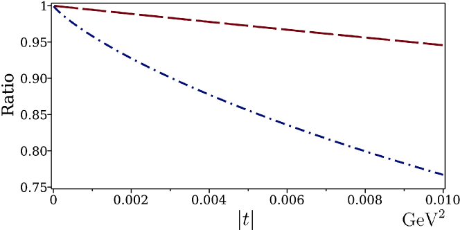
Figure 1: Ratios of the differential cross sections with amplitudes (19) [dashed curve] and (20) [dot-dashed curve] to the differential cross section for scattering of point-like particles.

So, in the case of proton scattering the difference is significant. This means that it is not reasonable to use the potential approach to describe CNI effect in proton scattering at the LHC. At the same time, in the region $|t|\lesssim 2\times 10^{-4}\,\mbox{GeV}^{2}$, where the Pb-Pb Coulomb scattering is occurring in the same mode, the difference between the two approaches is less than 1%. This means that the description of Pb-Pb Coulomb scattering in the indicated region is practically indistinguishable in both approaches.

3.2 Composite extended particles

As the transferred momenta increase from the above values, the internal structure of colliding particles becomes increasingly significant and the mode of multiple scattering on their charged components becomes prevailing. This mode was described by Glauber [14] in relation to the elastic scattering due to strong interactions of a fast point-like particle off a nucleus composed of nucleons. However, a generalization to the case of nucleus-nucleus scattering has not yet been found in a compact form. Below we construct the corresponding generalization applicable to Coulomb scattering of composite particles, using the terms of nuclear physics for definiteness. A special case of hadron scattering in this mode, we consider in the next subsection.

So, following the Glauber theory, we assume that protons in colliding nuclei are “frozen” as they pass each other, and the impacts of any proton of one nucleus on protons of another nucleus are independent of each other. The former condition means that nuclei are characterized by certain positions of the protons in the transverse projection. The latter condition means the absence of interaction correlations. In this case, the eikonal phase is the sum of individual phase shifts,

$$\delta_{ab}^{C}({\bf b},\{{\bf s}_{a},{\bf s}_{b}\})=\sum_{{}^{i=1,\dots N_{a}}_{j=1,\dots N_{b}}}\delta^{C}({\bf b}-{\bf s}_{a_{i}}\!+{\bf s}_{b_{j}})\,.$$ (21)

Here ${\bf s}_{a_{i}}$ and ${\bf s}_{b_{j}}$ are the positions of the protons $i$ and $j$ in the transverse projection relative to the centers of scattering nuclei $a$ and $b$, respectively, $N_{a}$ and $N_{b}$ are the numbers of charged protons inside them, and $\delta^{C}$ is the elementary Coulomb shift (7). For a given eikonal phase, the scattering amplitude operator acting in the space of variables $\{{\bf s}_{a},{\bf s}_{b}\}$ is defined as

$$F^{C}(s,q^{2};\{{\bf s}_{a},{\bf s}_{b}\})=\frac{s}{4\pi\mbox{i}}\int\!\mbox{d}^{2}{\bf b}\,e^{\mbox{\scriptsize{i}}{\bf q}{\bf b}}\left[e^{2\mbox{\scriptsize{i}}\delta_{ab}^{C}({\bf b},\{{\bf s}_{a},{\bf s}_{b}\})}-1\right].$$ (22)

The actual amplitude is determined by averaging (22) with the square of the product of wave functions of colliding particles. Practically this means taking integrals $\mbox{d}^{2}\{{\bf s}_{a_{i}}\!\}$ and $\mbox{d}^{2}\{{\bf s}_{b_{j}}\!\}$ of (22) with weights defined as the distributions of proton charges that specify the probability distribution of photon emission and absorption. So, the actual amplitude is

$$\displaystyle F^{C}(s,q^{2})=\int\mbox{d}^{2}\{{\bf s}_{a}\}\mbox{d}^{2}\{{\bf s}_{b}\}\;\varrho_{a}(\{{\bf s}_{a}\})\varrho_{b}(\{{\bf s}_{b}\})\,F^{C}(s,q^{2};\{{\bf s}_{a},{\bf s}_{b}\}).$$ (23)

Here $\mbox{d}^{2}\{{\bf s}_{\kappa}\}=\mbox{d}^{2}{\bf s}_{\kappa_{1}}\dots\mbox{d}^{2}{\bf s}_{\kappa_{N_{\kappa}}}$, $\varrho_{\kappa}(\{{\bf s}_{\kappa}\})=\varrho_{\kappa}({\bf s}_{\kappa_{1}},\dots\bf s_{\kappa_{N_{\kappa}}})$, where $\kappa=a,b$ and $\varrho_{\kappa}$ is the multi-proton density normalized to unity,

$$\int\mbox{d}^{2}\{{\bf s}_{\kappa}\}\,\varrho_{\kappa}(\{{\bf s}_{\kappa}\})=1\,.$$ (24)

Following [14], we further assume that the protons are distributed uncorrelatedly and their spatial densities are factorized:

$$\varrho_{\kappa}(\{{\bf s}_{\kappa}\})=\prod_{i=1,\dots N_{\kappa}}\hat{\rho}_{\kappa_{i}}({\bf s}_{\kappa_{i}}\!)\,,$$ (25)

where $\hat{\rho}_{\kappa_{i}}({\bf s}_{\kappa_{i}}\!)$ are the one-proton densities normalized to 1.

In terms of the profile functions of the Coulomb interaction of the protons

$$\gamma^{C}({\bf b}-{\bf s}_{a_{i}}+{\bf s}_{b_{j}})=e^{2\mbox{\scriptsize{i}}\delta^{C}({\bf b}-{\bf s}_{a_{i}}+{\bf s}_{b_{j}})}-1$$ (26)

the scattering amplitude operator (22) is written as

$$F^{C}(s,q^{2};\{{\bf s}_{a_{i}},{\bf s}_{b_{j}}\})=\frac{s}{4\pi\mbox{i}}\int\mbox{d}^{2}{\bf b}\;e^{\mbox{\scriptsize{i}}{\bf q}{\bf b}}\left\{\prod_{i=1}^{N_{a}}\prod_{j=1}^{N_{b}}\left[1+\gamma^{C}({\bf b}-{\bf s}_{a_{i}}+{\bf s}_{b_{j}})\right]-1\right\}.$$ (27)

Then amplitude (23) takes the form

$$F^{C}(s,q^{2})=\frac{s}{4\pi\mbox{i}}\int\mbox{d}^{2}{\bf b}\;e^{\mbox{\scriptsize{i}}{\bf q}{\bf b}}\;\Gamma^{C}({\bf b})\,,$$ (28)

where $\Gamma^{C}({\bf b})$ is the Coulomb profile function of the scattering nuclei,

$$\!\Gamma^{C}({\bf b})=\int\mbox{d}^{2}\{{\bf s}_{a}\}\mbox{d}^{2}\{{\bf s}_{b}\}\;\varrho_{a}(\{{\bf s}_{a}\})\varrho_{b}(\{{\bf s}_{b}\})\prod_{i=1}^{N_{a}}\prod_{j=1}^{N_{b}}\left[1+\gamma^{C}({\bf b}-{\bf s}_{a_{i}}+{\bf s}_{b_{j}})\right]-1.$$ (29)

Opening square brackets in (29), we obtain an expansion in the number of interactions of the protons. Symbolically, it has the form

$$\Gamma^{C}({\bf b})=\left\{\gamma^{C}\right\}+\left\{\gamma^{C}\gamma^{C}\right\}+\left\{\gamma^{C}\gamma^{C}\gamma^{C}\right\}+\cdots$$ (30)

Here the first term is the coherent sum of contributions from single elastic scatterings, the terms with two $\gamma^{C}$ are contributions from twofold scatterings, etc.

Formula (29) describes the general structure of the elastic scattering profile function in the case of multiple Coulomb scattering. A similar formula takes place in the case of nuclear scattering due to strong interactions. Unfortunately, contributions with a number of profile functions greater than 2 are characterized by very complicated combinatorics and are analytically resolved only for the lightest nuclei with a number of nucleons $\leq 4$ [17]. If the nuclei are heavier, then either the Monier-Carlo method or some approximation must be used.

For heavy nuclei, the so-called optical approximation was proposed [15, 16], which implies a formal transition to an infinite number of nucleons. In view of this, it is sometimes believed that for a large number of nucleons this approximation defines the leading contribution to the amplitude. This is certainly true if a point-like particle is scattered off a nucleus. However, in the case of scattering of two composite objects on each other a certain set of contributions that do not contain any small parameters is discarded in this approximation [18, 19]. Below we show that in the case of Coulomb scattering such a small parameter does exist and it is the fine structure constant $\alpha$.

So, following the general methodology of Glauber theory, we assume that all one-proton densities are the same, and introduce the charge density of the nucleus containing $N_{\kappa}$ protons,

$$\rho_{\kappa}({\bf s})=N_{\kappa}\times\hat{\rho}_{\kappa}({\bf s})\,.$$ (31)

So, $\rho_{\kappa}({\bf s})$ is normalized to $N_{\kappa}$, and $N_{\kappa}$ is the charge number of the nucleus. Given (31) and taking into account (25), we write (29) as

$$\Gamma^{C}({\bf b})=\int\mbox{d}^{2}\{{\bf s}_{b}\}\varrho_{b}(\{{\bf s}_{b}\})\left[1+\frac{1}{N_{a}}\int\mbox{d}^{2}{\bf s}_{a}\,{\rho_{a}}({\bf s}_{a})\,\Gamma^{C}_{N_{b}}({\bf b}-{\bf s}_{a};\{{\bf s}_{b}\})\right]^{N_{a}}\!\!-1\,.$$ (32)

Here ${\bf s}_{a}$ is an integration variable in the product of $N_{a}$ identical integrals, and

$$\Gamma^{C}_{N_{b}}({\bf b}-{\bf s}_{a};\{{\bf s}_{b}\})=\prod_{j=1}^{N_{b}}[1+\gamma^{C}({\bf b}-{\bf s}_{a}+{\bf s}_{b_{j}})]-1\,.$$ (33)

If $N_{a}$ is large enough, then integrand in (32) is well approximated by the exponent, and we arrive at

$$\Gamma^{C}({\bf b})=\int\mbox{d}^{2}\{{\bf s}_{b}\}\varrho_{b}(\{{\bf s}_{b}\})\,\exp\!\left[\int\mbox{d}^{2}{\bf s}_{a}\,{\rho_{a}}({\bf s}_{a})\Gamma^{C}_{N_{b}}({\bf b}-{\bf s}_{a};\{{\bf s}_{b}\})\right]-1\,.$$ (34)

This transformation is called the optical approximation in Glauber theory. In the given case, it was done for proton contributions of the nucleus $a$. A remarkable property of (34) is the disappearance of the dependence on $N_{a}$ and the transition of charge density ${\rho_{a}}({\bf s}_{a})$ to the exponent. This can be interpreted in such a way that protons of nucleus $a$ form a kind of continuous medium (cloud) on which the protons of nucleus $b$ are scattered. Accordingly, the expression in the exponent in (34) can be considered as the phase shift of this scattering.

Now we linearize $\Gamma^{C}_{N_{b}}({\bf b}-{\bf s}_{a};\{{\bf s}_{b}\})$ in (34) with respect to the fine structure constant $\alpha$, i.e. retain in the phase shift in (34) only the leading term in its expansion in powers of $\alpha$. Then due to (26) and (33) expression (34) takes the form

$$\Gamma^{C}({\bf b})=\int\mbox{d}^{2}\{{\bf s}_{b}\}\varrho_{b}(\{{\bf s}_{b}\})\,\exp\!\left[2\mbox{i}\!\int\!\mbox{d}^{2}{\bf s}_{a}\,{\rho_{a}}({\bf s}_{a})\sum_{j=1}^{N_{b}}\delta^{C}({\bf b}-{\bf s}_{a}+{\bf s}_{b_{j}})\right]-1\,.$$ (35)

It is worth noting that as a result of the linearization, each proton of nucleus $b$ interacts with the cloud of protons of nucleus $a$ only once.

Next, we introduce the profile function of scattering of protons of nucleus $b$ on the above-mentioned charged cloud of the nucleus $a$,

$$\bar{\gamma}^{C}_{a}({\bf b}+{\bf s}_{b_{j}})=\exp\!\left[2\mbox{i}\!\int\!\mbox{d}^{2}{\bf s}_{a}\,{\rho_{a}}({\bf s}_{a})\,\delta^{C}({\bf b}-{\bf s}_{a}+{\bf s}_{b_{j}})\right]-1\,,$$ (36)

and rewrite (35) in the form

$$\Gamma^{C}({\bf b})=\int\mbox{d}^{2}\{{\bf s}_{b}\}\varrho_{b}(\{{\bf s}_{b}\})\,\prod_{j=1}^{N_{b}}\left[1+\bar{\gamma}^{C}_{a}({\bf b}+{\bf s}_{b_{j}})\right]-1.$$ (37)

Passing, in accordance with (25) and (31) to the charge distribution density of nucleus $b$, we arrive at

$$\Gamma^{C}({\bf b})=\left[1+\frac{1}{N_{b}}\int\mbox{d}^{2}{\bf s}_{b}\,{\rho_{b}}({\bf s}_{b})\,\bar{\gamma}^{C}_{a}({\bf b}+{\bf s}_{b})\right]^{N_{b}}\!\!-1\,.$$ (38)

Passing, in turn, to the optical approximation in (38) and linearizing $\bar{\gamma}^{C}_{a}$ in $\alpha$, we obtain

$$\Gamma^{C}({\bf b})=\exp\!\left[2\mbox{i}\!\int\!\mbox{d}^{2}{\bf s}_{a}\mbox{d}^{2}{\bf s}_{b}\;\rho_{a}({\bf s}_{a})\rho_{b}({\bf s}_{b})\,\delta^{C}({\bf b}-{\bf s}_{a}+{\bf s}_{b})\right]-1\,.$$ (39)

This formula defines the leading non-trivial contribution to the Coulomb profile function of heavy nuclei. Note that the symmetry between $a$ and $b$ is restored, both charge density functions are exponentiated, and the dependence on the number of protons in the scattered nuclei disappears.

Based on (39) and (28), we arrive at the final result for the scattering amplitude, which repeats formula (13) but with $\delta^{C}_{ab}(b)$ defined using the densities $\rho_{a}({\bf s}_{a})$ and $\rho_{b}({\bf s}_{b})$ normalized to $N_{a}$ and $N_{b}$, respectively. Since the formulas for the amplitude coincides, the elimination of IR divergences is carried out in the same way as in the previous subsection.

In conclusion, we recall that in the previous subsection formula (13) was obtained in the potential approach in the case of particles as structurless objects with a continuous charge distribution. Here we obtained this formula in the QFT approach in a different kinematic region and in a different scattering mode, when the scattering occurs on a large number of charged components of the particles. The coincidence of the final formula here with the previous one occurred after a double transition to the optical approximation and linearization in $\alpha$ of the resulting phase shift. Performing these operations twice leads to an effective scattering pattern as a scattering of charged clouds with a continuous charge distribution. What is important is that this pattern corresponds to the leading approximation for Coulomb scattering of heavy nuclei.

3.3 Hadrons as composite extended particles

The case of elastic Coulomb scattering of hadrons on charged partons is in many ways analogous to the case with nuclei considered above. However, there are differences due to the fact that the number of partons in fast-moving hadrons is not fixed and the partons have different electric charges. In this regard, we introduce to the eikonal phase the electric charges $\varepsilon_{i}$ and $\varepsilon_{j}$ of the partons in units of $\sqrt{\alpha}$. So instead of (21) we write

$$\delta_{ab}^{C}({\bf b},\{{\bf s}_{a},{\bf s}_{b}\})=\sum_{{}^{i=1,\dots N_{a}}_{j=1,\dots N_{b}}}\varepsilon_{i}\varepsilon_{j}\,\delta^{C}({\bf b}-{\bf s}_{a_{i}}\!+{\bf s}_{b_{j}})\,.$$ (40)

Furthermore, since the number of partons is not fixed, the amplitude is now defined as

$$F^{C}(s,q^{2})=\sum_{\{N_{a}\},\{N_{b}\}}W_{\{N_{a}\}}W_{\{N_{b}\}}\;F^{C}_{\{N_{a},N_{b}\}}(s,q^{2})\,,$$ (41)

where

$$F^{C}_{\{N_{a},N_{b}\}}(s,q^{2})=\int\mbox{d}^{2}\{{\bf s}_{a}\}\mbox{d}^{2}\{{\bf s}_{b}\}\;\varrho_{a}(\{{\bf s}_{a}\})\varrho_{b}(\{{\bf s}_{b}\})\,F^{C}(s,q^{2};\{{\bf s}_{a},{\bf s}_{b}\})\,.$$ (42)

Here $\{N_{\kappa}\}$ is a certain set of $N_{\kappa}$ charged partons. The probabilities $W_{\{N_{\kappa}\}}$ satisfy the conditions $\sum_{\{N_{\kappa}\}}W_{N_{\{N_{\kappa}\}}}=1$, where the summation is performed over the specific sets and the numbers of partons in the sets.

In accordance with (40), the profile functions of the Coulomb interaction of the partons we now define as,

$$\gamma^{C}_{ij}({\bf b}-{\bf s}_{a_{i}}+{\bf s}_{b_{j}})=e^{2\mbox{\scriptsize{i}}\varepsilon_{i}\varepsilon_{j}\delta^{C}({\bf b}-{\bf s}_{a_{i}}+{\bf s}_{b_{j}})}-1\,.$$ (43)

Accordingly, the partial amplitude (42) is written as

$$F^{C}_{\{N_{a},N_{b}\}}(s,q^{2})=\frac{s}{4\pi\mbox{i}}\int\mbox{d}^{2}{\bf b}\;e^{\mbox{\scriptsize{i}}{\bf q}{\bf b}}\;\Gamma^{C}_{\{N_{a},N_{b}\}}({\bf b})\,,$$ (44)

where $\Gamma^{C}_{\{N_{a},N_{b}\}}({\bf b})$ is the partial profile function of scattering hadrons,

$$\!\Gamma^{C}_{\{N_{a},N_{b}\}}({\bf b})=\int\mbox{d}^{2}\{{\bf s}_{a}\}\mbox{d}^{2}\{{\bf s}_{b}\}\;\varrho_{a}(\{{\bf s}_{a}\})\varrho_{b}(\{{\bf s}_{b}\})\prod_{i=1}^{N_{a}}\prod_{j=1}^{N_{b}}\left[1+\gamma^{C}_{ij}({\bf b}-{\bf s}_{a_{i}}+{\bf s}_{b_{j}})\right]-1.$$ (45)

In view of the need for subsequent averaging over the sets of partons, the combinatorics in (45) must be resolved for arbitrary $N_{a}$ and $N_{b}$. However, in the general case this is hardly possible. So, apparently the only way to obtain a workable solution is to use the optical approximation, which implies effective disappearance of the dependence on $N_{a}$ and $N_{b}$. Unfortunately, the condition of a large number of scattering components faces a serious problem in the case of hadrons.

Really, in a proton at rest the average number of charged partons is 3. In a fast-moving proton their average number is increasing with increasing the energy (due to the increase in the length of parton splitting cascades). In collisions with increasing $q^{2}$ the effect of parton dissociation is additionally activated. However, in both cases the growth of the average number of partons is very slow (logarithmic). As a result, with restricted momentum transfers the condition for the applicability of the optical approximation in the case of hadrons is extremely high collision energies. Moreover, the energies must be so high that they can hardly be achieved at colliders. Nevertheless, if there is an effect, it is worth studying.

So, we proceed to constructing the optical approximation in the case of Coulomb scattering of hadrons. We will carry out the analysis in two stages. At the first stage, as a methodological technique, we assume that the colliding hadrons $a$ and $b$ contain partons of only one type, i.e. their partons have common charges and common one-parton densities, although in different hadrons they may be different. In this case the charges of our hypothetical hadrons are $N_{\kappa}\times\varepsilon_{\kappa}$, where $\kappa=a,b$, and their charge distribution densities in units of $\varepsilon_{\kappa}\sqrt{\alpha}$ are enhanced by $N_{\kappa}$ times the one-parton densities,

$$\widetilde{\rho_{\kappa}}({\bf s})=N_{\kappa}\times\hat{\rho}_{\kappa}({\bf s})\,.$$ (46)

So, $\widetilde{\varrho_{\kappa}}({\bf s})$ are normalized to $N_{\kappa}$. Here the tilde means that we are considering hypothetical particles. Given (46) and repeating the calculations of the previous subsection, we arrive at the following expression for the partial profile function,

$$\Gamma^{C}_{\{N_{a},N_{b}\}}({\bf b})=\exp\!\left[\int\!\mbox{d}^{2}{\bf s}_{a}\mbox{d}^{2}{\bf s}_{b}\;\widetilde{\rho_{a}}({\bf s}_{a})\widetilde{\rho_{b}}({\bf s}_{b})\,2\mbox{i}\varepsilon_{a}\varepsilon_{b}\,\delta^{C}({\bf b}-{\bf s}_{a}+{\bf s}_{b})\right]-1\,.$$ (47)

At the second stage, we return to the case of real hadrons. Namely, we “allow” them to consist of partons of certain types and charges. At the same time, we require that the number of partons of each type be large enough. This will allow us to go to the optical approximation separately for each group of partons. In this case, under the exponent sign in the corresponding analogue of formula (47) the sum of contributions of partons of all types will appear. (The transition to the real case can be made first for one particle and then for another.) As a result, $\varepsilon_{a}\widetilde{\rho_{a}}({\bf s}_{a})\,\varepsilon_{b}\widetilde{\rho_{b}}({\bf s}_{b})$ in (47) will move into the sum of the products of contributions of groups of partons of certain types, and then into the product of charge densities of real hadrons:

$$\varepsilon_{a}\widetilde{\rho_{a}}({\bf s}_{a})\,\varepsilon_{b}\widetilde{\rho_{b}}({\bf s}_{b})\;\longrightarrow\;\sum_{I}\varepsilon_{a_{I}}\rho_{a_{I}}({\bf s}_{a})\sum_{J}\varepsilon_{b_{J}}\rho_{b_{J}}({\bf s}_{b})={\rho}_{a}({\bf s}_{a}){\rho}_{b}({\bf s}_{b})\,.$$ (48)

Here, in the middle expression summation is carried out over the groups of partons, and $\rho_{\kappa_{I}}({\bf s}_{\kappa})$ are the charge distribution densities of the groups. In the final expression ${\rho}_{\kappa}({\bf s})=\sum_{I}\varepsilon_{\kappa_{I}}\rho_{\kappa_{I}}({\bf s})$, which is the charge density of the real hadron $\kappa$ in units of $\sqrt{\alpha}$.

Now note that due to the absence of dependence on $\{N_{a}\}$ and $\{N_{b}\}$ in the final formula for the partial profile function, which is obtained by combining (47) and (48), the partial amplitude (44) is also independent of $\{N_{a}\}$ and $\{N_{b}\}$. Hence, averaging with probabilities $W_{\{N_{a}\}}$ and $W_{\{N_{b}\}}$ in (41) is trivial.

So, we again arrive at formula (13), in this case for the amplitude of Coulomb scattering of hadrons as structured composite particles. The $\delta^{C}_{ab}(b)$ in this formula is defined with the charge densities of real hadrons, as defined above. Our concluding remarks repeat the last paragraph of the previous subsection, with “heavy nuclei” replaced by “hadrons at extremely high energies”.

4 Discussion and conclusion

We have carried out a description of high-energy Coulomb elastic scattering of extended particles in three scattering modes determined by the magnitude of the momentum transfer, and we have compared the predictions of the eikonal model in the potential and QFT approaches.

In the limit of small transfers, particles are scattered as point-like objects, and the description of their scattering coincides in the potential and QFT versions of the eikonal model. In essence, this is a trivial result, and we present it for completeness. However, if the wavelength of the exchanged photons becomes comparable to the size of the particles, then the scattering occurs immediately on all charged parts of the colliding particles. In the case of protons, this scattering mode occurs at $q^{2}\lesssim 10^{-2}\,\mbox{GeV}^{2}$. (In this region CNI effect is significant at the LHC energies.) In the case of nuclei, a similar limitation is determined by the value inverse to their transverse sizes. For example, in the case of Pb-Pb scattering a similar estimate is $q^{2}<2\times 10^{-4}\,\mbox{GeV}^{2}$. Coulomb scattering in this mode is described differently in the potential and QFT versions of the eikonal model. The difference manifests itself in different ways of accounting for electromagnetic form factors. The reason for the difference is related to the relativistic non-invariance of the Schrödinger equation which underlies the potential approach. In particular, the expression for the kinetic energy of particles of the type $\vec{\,p}^{\,2}/2m$ is incorrect in the relativistic region. However, this expression is used significantly in the derivation of formula (3) for the eikonal shift. At the same time, the relativistic non-invariance of the potential is irrelevant. In classical electrodynamics it transforms in a covariant manner, and this effect together with the potential retardation effect, can be consistently taken into account. Both of them do not affect the eikonal shift due to the integration of the potential in formula (3) over the longitudinal coordinate. In quantitative terms, the difference between the descriptions in the potential and QFT approaches is significant in the CNI region in the case of proton scattering at the LHC. We interpret this as an inappropriateness of the potential approach to the description of the proton Coulomb scattering. At the same time, in the case of Coulomb scattering of heavy nuclei in the relevant region of the momentum transfer, the quantitative discrepancy between the descriptions in the above approaches is insignificant.

As $q^{2}$ increases from the above specified values, the Coulomb scattering gradually switches to the mode with scattering on individual charged components of colliding particles. As a result, the scattering takes on a multiple character, which is described by Glauber theory. In the case of nuclei, the mentioned components are first protons and with further increase in $q^{2}$ are charged partons in the nucleons. If nuclei contain a large number of protons, then in both cases the amplitude is determined by formula (13) with the modification indicated in the end of Section 3.2. The essential innovation achieved in this study is that this formula in the case of Coulomb scattering of heavy nuclei actually defines the leading approximation for the amplitude.

In hadron collisions, the situation with increasing $q^{2}$ beyond the limit specified above is more complicated, since in this case an analogue of a large number of protons in nuclei is a large number of charged partons in the colliding hadrons. For restricted $q^{2}$ this can be achieved at extremely high collision energies, certainly above 100 TeV, since the growth with the energy of the average number of partons is very slow (logarithmic). At realistic energies achievable at colliders, Coulomb scattering of hadrons falls into an intermediate zone, in which a compact solution has not yet been found. Fortunately, the solution in this region has no practical significance, since at $q^{2}>10^{-2}\,\mbox{GeV}^{2}$ the Coulomb interaction of hadrons becomes negligible against the background of their strong interactions. Nevertheless, theoretical description of this scattering mode is of interest, because it sheds light on the conditions under which the potential scattering formula could become relevant for describing Coulomb scattering of hadrons.

In conclusion, we recall that in the region of very small momentum transfers Coulomb contributions become dominant in the elastic scattering of strongly interacting charged particles. In this regard, description of the Coulomb scattering is an essential component of the study of hadron interactions. Meanwhile, until now there was no understanding of how to correctly take into account the finite sizes of colliding particles when describing their Coulomb interactions. There was also no understanding whether the use of the optical approximation in describing Coulomb scattering of heavy nuclei was correct. This work brings a certain clarity to these issues.

Acknowledgments: The author is grateful to V.A. Petrov for stimulating discussions.

References

- [1] H. Bethe, Ann. Phys. 3 (1958) 190.
- [2] L.D. Solov’ev, JETP 22 (1966) 205.
- [3] G.B. West, D.R. Yennie, Phys. Rev. 172 (1968) 1413.
- [4] M.M. Islam, Phys. Rev. 162 (1967) 1426.
- [5] R. Cahn, Z. Phys. C15 (1982) 253.
- [6] V. Kundrát, M. Lokajiček, Z. Phys. C 63 (1994) 619.
- [7] V.A. Petrov, Eur. Phys. J. C 78 (2018) 221, [Erratum, Eur.Phys.J. C 78 (2018) 414].
- [8] L. Durand, P. Ha, Phys. Rev. D 102 (2020) 036025.
- [9] J. Kašpar, Acta Phys. Pol. B 52 (2021) 85.
- [10] V.A. Petrov, N.P. Tkachenko, Nucl. Phys. A 1042 (2024) 122807.
- [11] M.L. Nekrasov, Phys. Lett. B 849 (2024) 138485.
- [12] H. Cheng, T.T. Wu, Phys. Rev. 186 (1969) 1611.
- [13] M. Lévy, J. Sucher, Phys. Rev. 186 (1969) 1656.
- [14] R.J. Glauber, Lectures in Theoretical Physics, Vol. I, edited by W.E. Brittin et al. (Interscience, N.Y., 1959) p. 315.
- [15] W. Czyz and L.C. Maximon, Ann. Phys. 52 (1969) 59.
- [16] J. Formánek, Nucl. Phys. B 12 (1969) 441.
- [17] V. Franco, Phys. Lett. B 64 (1976) 13.
- [18] I.V. Andreev and A.V. Chernov, Yad. Fiz. 28 (1978) 477.
- [19] K.G. Boreskov and A.B. Kaidalov. Yad. Fiz. 48 (1988) 575.
- [20] Yu.M. Shabelski, A.G. Shuvaev, Phys. Rev. C 104 (2021) 064607.
- [21] G.Z. Moliere, Naturforsch, 1947, 2A, 133
- [22] J. Kašpar, V. Kundrát, M. Lokajiček, J. Procházka, Nucl. Phys. B 843 (2011) 84.
- [23] G. Antchev et al. (TOTEM Collaboration), Eur. Phys. J. C76 (2016) 661.
- [24] G. Antchev et al. (TOTEM Collaboration), Eur. Phys. J. C 79 (2019) 785.
- [25] M.L. Nekrasov, Mod. Phys. Lett. A 35 (2020) 2050314.
- [26] M.L. Nekrasov, Particles 4 (2021) 381.
- [27] M.L. Nekrasov, Phys. Rev. D 106 (2022) 014028.
- [28] A.V. Tarasov, Fiz.Elem.Chast.Atom.Yadra 7 (1976) 771.