On sums of dependent random lifetimes under the Time Transformed Exponential model
Abstract
Considered a pair of random lifetimes whose dependence is described by a Time Transformed Exponential model, we provide analytical expressions for the distribution of their sum. These expressions are obtained by using a representation of the joint distribution in terms of multivariate distortions, which is an alternative approach to the classical copula representation. Since this approach allows to obtain conditional distributions and their inverses in simple form, then it is also shown how it can be used to predict the value of the sum from the value of one of the variables (or vice versa) by using quantile regression techniques.
Keywords: Dependence models, C-convolution, distorted distributions, quantile regression, confidence bands.
1 Introduction
Let be a pair of dependent lifetimes. The vector is said to be described by a Time Transformed Exponential model (shortly, TTE model) if its joint survival function can be written as
| (1.1) |
for a suitable one-dimensional, continuous, convex and strictly decreasing survival function and two suitable continuous and strictly increasing functions such that and , for . Clearly, the marginal survival functions for the lifetimes are given by , , .
TTE models have been considered in literature as an appropriate manner to describe bivariate lifetimes (see, e.g., [1, 8, 13] and references therein). Their main characteristic is that they “separate”, in a sense, aging of single lifetimes through the functions , and dependence properties through , the copula being a transformation of only (see Eq. (2) below and the reference above for details). This model is of interest in a variety of applicative fields since it is equivalent to the random frailty model, which assumes that the two lifetimes are conditionally independent given a random parameter that represents the risk due to a common environment; the well-known proportional hazard rate Cox model, where the proportional factor is not fixed but random, is an example. In this case, the different choices for the function are obtained just by changing the distribution of random parameter.
For a number of applicative purposes, one can be interested in the sum . This happens, for example, in considering the total lifetime in stand-by systems, where a component is replaced by a new one under the same environmental stress after its failure, or in insurance theory, where the sum of two depended claims, due to common risks, may be evaluated. In this case, because of the dependence between and , the classical convolution can not be applied to determine the distribution of , and C-convolutions must be used (see, e.g., [2, 4, 17] for definition and examples of C-convolutions). That is, one can calculate the survival function of as
| (1.2) |
where and are the marginal survival functions of and , respectively, is the density function of (assuming its existence) and is the survival copula of the vector . Here, means the partial derivative of with respect to its first argument. Note that, in particular, for nonnegative random variables Eq. (1.2) reduces to
Since usually the integrals appearing in previous formulas are not easy to be solved, we describe in this paper an alternative tool to deal with the sum that can be used when the joint distribution of is defined as in Eq. (1.1). This approach is based on an alternative representation for the survival function of , which make use of the distortion representations of multivariate distributions recently introduced in [11], whose definition is provided in the next section. The advantage of this approach is twofold: it is particularly useful when the inverse of is not available in closed form, thus also , and it also provides simple representations of the conditional distribution of given one of the , and of its inverse, so that one can use it to predict the value of the sum from the value of one of the variables (or vice versa) by using quantile regression techniques. The purpose of this paper is to describe such an approach.
The rest of the paper is structured as follows. Basic definitions, notations and some preliminary results are introduced in Section 2. The main results for the representation of the distribution of the sum are provided in Section 3, while examples of their application in prediction are presented in Section 4 and Section 5.
Throughout the paper the notions increasing and decreasing are used in a wide sense, that is, they mean non-decreasing and non-increasing, respectively, and we say that is increasing (decreasing) if for all (where this last inequality means that for every -th component of the vectors one has ). Also, if is a real valued function in more than one variables, then denotes the partial derivative of with respect to its -th variable. Analogously, and so on. Whenever we use a partial derivative we are tacitly assuming that it exists.
2 Notation and preliminary results
To simplify the notation we just consider here the bivariate case; the extension to the -dimensional case is straightforward. Moreover, we just consider nonnegative random variables with absolutely continuous distributions even if many of the properties described below can be extended to arbitrary random variables.
Thus, let be a random vector with two possibly dependent nonnegative random variables having an absolutely continuous joint distribution function and marginal distributions and . Let be the joint probability density function (PDF) of and let and be the PDFs of and , respectively. Then it is well known (see, e.g., [18]) that, from Sklar’s Theorem, there exists a unique absolutely continuous copula such that can be written as
| (2.1) |
for all . As a consequence, the PDF function can be obtained as
where is the PDF of the copula . A similar representation holds for the joint survival function
for all , where and are the marginal survival functions and is another suitable copula, called survival copula.
In the particular case of TTE models, i.e., in the case that the joint survival function is defined as in Eq. (1.1), then the corresponding survival copula is the strict bivariate Archimedean copula (see, e.g., [18], p. 112) defined as
for all . This model contains many families of copulas (see, [18], p. 117), thus it is a very general dependence model. The inverse function is called the additive generator of the copula..
However, an alternative representation of based on distortion representations of multivariate distributions can be given. In some cases, and for specific applications, such an alternative representation can be preferable to classical copula approach.
For it first recall that a function is said to be a distortion function if it is continuous, increasing and satisfies and . If is a distribution function, we say that is a distorted distribution from if there exists a distortion function such that for all , and similarly for the survival functions. This kind of representations were introduced in the theory of decision under risk (see e.g. [20, 21]) and they were also applied in the fields of coherent systems, order statistics and conditional distributions (see, e.g., [12, 16] and the references therein).
These representations were further extended to the multivariate case in the recent paper [11]. According to what defined there, and restricting to the bivariate case, a function is a bivariate distortion if it is a continuous -dimensional distribution with support included in , and a bivariate distribution function is a distortion of the univariate distribution functions and if there exists a bivariate distortion such that
| (2.2) |
for all .
This representation is similar to the copula representation, but here the are not necessarily the marginal distribution of and is not necessarily a copula. Actually, in some situations, we can choose a common univariate distribution , and some examples will be provided later (see also [10, 11]). Moreover, if has uniform univariate marginal distributions over the interval , then is a copula, are the marginal distributions and (2.2) is the same as the copula representation (2.1) (but only in this case).
The main properties of model (2.2) were given in [11] and they are very similar to that of copulas. For example, if is a distortion function, then the right-hand side of (2.2) defines a proper multivariate distribution function for any univariate distribution functions and . Moreover, a similar representation holds for the joint survival function, that is, one can write
| (2.3) |
where , for , and is another suitable distortion function.
For TTE model note that, defining
| (2.4) |
one has
for all , where
| (2.5) |
The function satisfies the property to be a bivariate distortion if satisfies the properties mentioned above, i.e., if it is an absolutely continuous strictly decreasing convex function in with and . Note that if we add for , then is the survival function of a nonnegative random variable. Also note that and are two arbitrary survival functions satisfying . Thus, a representation through multivariate distortions as in (2.2) holds for the TTE models, with defined as in (2.5).
It must be pointed out that with this representation the marginal survival functions are not explicitly displayed, but can be obtained as
where , is a univariate distortion function. Finally, note that the representation through the multivariate distortion (2.5) and the univariate survivals (2.4) is a copula representation if and only if that is, for . This property leads to for and for which is the product copula that represents the independence case. For other (non-exponential) survival functions , we obtain models with dependent variables, whose dependence is described by .
As an interesting particular case, this dependence model includes the one recently proposed in [5] for nonnegative random variables, which is characterized (see Proposition 3.1 in [5]) by the joint survival function
| (2.6) |
for , where are two positive scale parameters and satisfies the above mentioned properties. This model, that from now on will be referred as GK-model (where the letters G and K indicates the initials of the authors Genev and Kolev of reference [5]) is an extension of the well known Schur-constant model which is obtained when (see [3] and references therein). Properties of this model and of the corresponding sum are studied also in [19]. It must be observed that the marginal survival functions are and for , and both of them belong to the scale parameter model defined by . Actually, this model is obtained by the distortion of univariate exponential distributions, i.e., if (2.6) holds, then
for all , where , and is defined as in Eq. (2.5).
3 Distribution and conditional distribution of the sum
In this section we use the distortion representation (2.3), with the multivariate distortion defined as in (2.5), to study the sum under the dependence model defined in the preceding section. As a consequence, we also obtain the analogous properties for the GK-model, i.e., the generalization (2.6) of the Schur-constant model.
Proposition 3.1.
Proof.
From (2.3), the joint PDF of is
for , where and . Then the joint PDF of is
for . The PDF of our specific distortion function is
and
for which concludes the proof. ∎
Remark 3.1.
In particular, for the GK-model in (2.6), that is, with exponential survival functions and with shape parameters (hazard rates) and , the PDF reduces to
for (zero elsewhere). Therefore its joint distribution function is
where . To solve this integral we consider two cases. If , then
| (3.2) |
while if , then
| (3.3) |
for . In both cases, (3.2) and (3.3) can be represented as distorted distributions from by replacing with and with .
In particular, as immediate consequence one can obtain the distribution of the sum (C-convolution) for the GK-model as
If , then
or if , then
for . Note that the first expression is a negative mixture (i.e. a linear combination with a negative weight) with PDF
| (3.4) |
for , where . In the second case, one gets
| (3.5) |
for , which is the expression in Remark 2.7 of [3] (i.e. for the Schur-constant model).
The joint survival function of under the model (2.3) and (2.5) in the non-exponential case for the is obtained in the following proposition. Unfortunately, an explicit expression can not be provided in general, but it is available in some cases, or easily available numerically (see the examples in the next sections).
Proposition 3.2.
Proof.
Therefore, the survival function of can be obtained as
| (3.6) |
and its PDF as .
To get the explicit expression for we need to explicitate and/or and to solve this integral, eventually numerically. For example, if for , then
and for which is the expression in Remark 2.7 of [3] for the Schur-constant model.
4 Predictions
The purpose of this section is to show how to predict the value of the sum from or vice versa by making use of the results in the previous section. To this purpose we need the conditional distribution of in the TTE dependence model, that is obtained in the following proposition.
Proposition 4.1.
Proof.
From (3.1), the PDF of is
for . Moreover, the first marginal survival function is
and its PDF is , for .
Hence, the PDF of for such that , can be obtained as
for (zero elsewhere).
Then the associated distribution function is
for and we conclude the proof. ∎
Hence, the conditional survival function is
Clearly, this is a distortion representation from , since
for , where
for is a distortion function for all .
Note that the inverse function of (i.e. its quantile function) can be obtained from the inverse functions of and as
| (4.2) |
for . The inverse function of can be obtained in a similar way.
One can thus predict from by using the quantile (or median) regression curve with
Moreover, one can compute the centered confidence bands for these estimations as
For example, the centered confidence band for is
Such an interval is computed below in some illustrative examples.
Remark 4.1.
In particular, for the GK-model in (2.6) we get
| (4.3) |
and
| (4.4) |
for and . Note that these expressions hold both for and for .
The other conditional distribution can be obtained in a similar manner. However, it is more difficult to get an explicit expression since we need the PDF of . It is stated in the following proposition.
Proposition 4.2.
Proof.
From (3.1), the PDF of is
for . Its second marginal survival function was obtained in (3.6). It can also be obtained as in (4.6).
Hence, the conditional PDF of is
Then the associated distribution function is the one given in (4.5) for and the assertion is proved. ∎
In particular, for the GK-model we have the following explicit expressions.
Proposition 4.3.
Proof.
From the preceding proposition we have
for (zero elsewhere). Its second marginal PDF function was obtained in (3.4) () and in (3.5) ().
In the first case we get
and in the second
for .
Then the associated distribution functions are
(in the first case) and
(in the second case) for . ∎
Note that the expression (4.8) was obtained previously in Proposition 2.3 of [3] for the Schur-constant model (which is equivalent to (2.6) with ).
As in the preceding case, expressions (4.7) and (4.8) can be used to obtain quantile regression curves to predict from . An illustrative example is given in the following section. In both cases, they can be represented as distorted distributions from by replacing with and with .
In the second case (), the inverse function is for and the trivial median regression curve is (which in this case coincides with the classic mean regression curve ).
5 Examples
In this section we provide some examples to illustrate the theoretical findings described in previous sections. In the first one we consider the sum of two dependent random variables satisfying the GK-model proposed in [5], i.e., the model (2.6).
Example 5.1.
Let us assume that satisfies (2.6) for and for (Pareto type II survival function) and . This model is equivalent to consider an Archimedean Clayton copula with and Pareto type II marginals. Then, from (3.2), the joint distribution function of is
for . Hence, the distribution function of (i.e. the C-convolution) is
for . Its PDF is
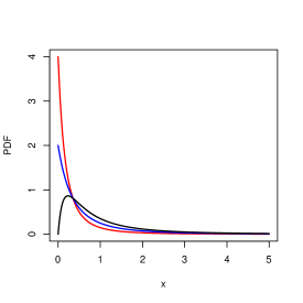
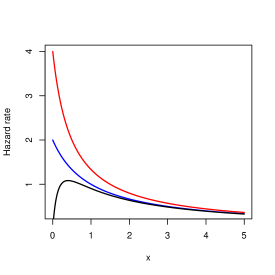
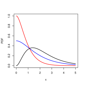
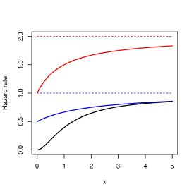
for . The distribution of is a negative mixture of two Pareto type II distributions and so its hazard rate goes to zero when (which is the limit of the hazard rates of the members of the C-convolution). They are plotted in Figure 1 (right) jointly with the associated PDF functions (left) for and . Note that the hazard rates of and are decreasing while the one of is not monotone (showing that the IFR class is not preserved by the sum of dependent r.v.).
If we want to predict from , we need the conditional distribution obtained from (4.7) as
for . Its inverse function is then
for . The median regression curve is obtained by replacing with . It is plotted in Figure 2, jointly with a sample from and the associated and centered confidence bands. We also include there the parametric (left) and non-parametric (right) estimations for these curves. Here, non-parametric means that we use the linear quantile regression procedure in R.
To estimate the parameters in the model from the sample we use recall the Kendall’s tau coefficient of is
(see [18], p. 163). Therefore, is estimated by
Then we recall that and to estimate and , obtaining
and
For the non-parametric linear estimators of the quantile regression curves, we used the R library quantreg (see [6, 7, 9]). The estimated median regression line to estimate from obtained from our sample is
The procedure to predict from is analogous.
In the next example we consider the general dependence model defined in (2.3) and (2.5). In this case we show how to predict from .
Example 5.2.
Recall that in (2.3) we assume that the joint survival function of can be written as
where and are two absolutely continuous survival functions with , while (2.5) asserts that
| (5.1) |
for , where satisfies the properties stated after Eq. (2.5). This model is a bivariate distorted distribution, for which the marginal survival functions are , for Thus, we can use the expressions obtained in Section 4, (4.1) and (4.2), to predict from .
For example, we can choose
for , where is the standard normal distribution and (i.e. is a truncated Normal distribution). Hence where is the PDF of a standard normal distribution. Note that, in this case, the associated Archimedean copula (that we could call Gaussian Archimedean copula) does not have an explicit expression (since it depends on and on ). Thus, this is a practical example where the distortion representation (5.1) can be used as a proper alternative.
Its inverse functions are
and
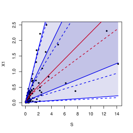
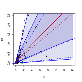
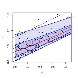
By using these expressions we compute as in (4.2), obtaining the quantile regression curve plotted in Figure 3, left. The same figure also includes a sample of points from and the exact centered and (blue) confidence bands. Moreover, it shows the plot of the non-parametric linear quantile estimate (dashed lines) obtained from this sample.
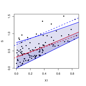
As we know that , we could also provide bottom and confidence bands obtained as and , respectively. They are plotted in Figure 3, right. In this case, the median regression curve is also the upper limit for the confidence band. In our sample we obtain data above the upper (exact) limit and above the median regression curve (i.e. data in the exact bottom confidence band). The estimated median regression line obtained from our sample is
for .
In the next example we show a case of model (2.6) that cannot be represented with an explicit Archimedean copula, thus for which the distortion representations consists in a useful alternative tool. In fact, in this example is convex and an explicit expression for its inverse is not available. For this model we compute the explicit expressions for the C-convolution and the two conditional survival functions.
Example 5.3.
Consider (2.6) with and the survival function
for . Its PDF is
for , that is, it is a translated Gamma (Erlang) distribution. The joint survival function of is
for . The marginals have also translated Gamma distributions.
The joint distribution of can be obtained from (3.2). From this expression, one can obtain the survival function of (C-convolution) as
for . Note that it is a negative mixture of two translated Gamma distributions.
The conditional survival function of can be obtained from (4.3) as
for . Analogously, from (4.7), the conditional survival function of is
for .
In Figure 4 we plot the probability density (left) and hazard rate (right) functions of (red), (blue) and (black) when and . Note that both marginals are IFR and the same holds for . Also note that the limiting behaviour of the hazard rate of coincides with that of the best component () in the sum. This is according with the results on mixtures obtained in Lemma 3.3 of [15] (or Lemma 4.6 in [17]) and that in Theorem 1 of [2] on usual convolutions.
In the last example we show a case dealing with the GK model (2.6) where the inverse of the conditional distribution function of cannot be obtained in a closed form. Then we need to use numerical methods (or implicit functions plots). It also shows that the quantile (median) regression curve is not always increasing.
Example 5.4.
Let us consider the model (2.6) which leads to a survival copula in the family of Gumbel-Barnett copulas (see (4.2.9) in [18], p. 116). In this case, the additive generator of the copula is for and . These copulas are strict Archimedean copulas and the independence (product) copula is obtained for . Hence,
and
for . Note that the inverse of has not an explicit form, thus one cannot use (4.9) to compute the quantile functions of . The same happens in (4.4) for the quantile functions of .
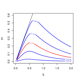
However, it is possible to plot the level curves of the conditional distribution function by using (4.7), obtaining
| (5.2) |
when . For example, if we choose , and in (5.4), we get
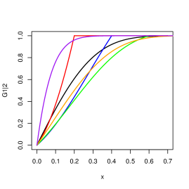
for . These level curves for are plotted in Figure 5, left. Note that the median regression curve (red line, left) is first increasing and then decreasing. To explain this surprising fact we plot in Figure 5, right, for different values of , where one can observe that these distribution functions are not ordered in , that is, is not stochastically increasing in . Here the greater values for are obtained when (green line). Also note that and that and are negatively correlated. Therefore, the greater values of are mainly obtained from the greater values of and the smaller values of . Thus is decreasing at the end.
Also note that
Therefore, when and, in particular, when and are independent. However, the covariance will be negative if . In our case, the marginal reliability functions of and are and , respectively. Their means are and , their variances and and their covariance . Hence
6 Conclusions
We formulated the TTE dependence model by using a distortion representation based on a specific fixed distortion function . This representation is useful to compute the joint distribution of and the sum , as well as to provide expressions for the survival function of and the conditional distributions of given or given . They can be used also to predict one value from the other by using quantile regression. Some examples illustrate these facts, showing that sometimes the classical copula approach can not be applied.
This paper is a first step on applications of distortion representations for dependence models. Thus, there are several tasks for future research. The main one could be to get explicit models by choosing appropriate functions , and , to study their main properties and how they fit to real data sets, allowing for the use of the prediction techniques developed here for these data sets. Other interesting questions deal with dependence models for which the multivariate distortion function differs from the one in Eq. (2.5), or how to get explicit expressions for the multivariate case.
Acknowledgements
JN and JM are supported by Ministerio de Ciencia e Innovación of Spain under grant PID2019-103971GB-I00/AEI/10.13039/501100011033. FP is partially supported by the grant Progetto di Eccellenza, CUP: E11G18000350001 and by the Italian GNAMPA research group of INdAM (Istituto Nazionale Di Alta Matematica).
References
- [1] Bassan B., Spizzichino F. (2005). Relations among univariate aging, bivariate aging and dependence for exchangeable lifetimes. Journal of Multivariate Analysis 93, 313–339.
- [2] Block H., Langberg N., Savits T. (2015). The limiting failure rate for a convolution of life distributions. Journal of Applied Probability 52, 894–898.
- [3] Caramellino L., Spizzichino F. (1994). Dependence and aging properties of lifetimes with Schur-constant survival functions. Probability in the Engineering and Informational Sciences 8, 103–111.
- [4] Cherubini U., Gobbi F., Mulinacci S. (2016). Convolution Copula Econometrics. Springer, Cham.
- [5] Genest C., Kolev N. (2021). A law of uniform seniority for dependent lives. Scandinavian Actuarial Journal 2021, 726–743. DOI: 10.1080/03461238.2021.1895299.
- [6] Koenker R. (2005). Quantile Regression. Cambridge University Press.
- [7] Koenker R., Bassett Jr, G. (1978). Regression quantiles. Econometrica 46, 33–50.
- [8] Mulero J., Pellerey F., Rodríguez-Griñolo R. (2010). Stochastic comparisons for time transformed exponential models. Insurance: Mathematics and Economics 46, 328–333.
- [9] Navarro J. (2020). Bivariate box plots based on quantile regression curves. Dependence Modeling 8, 132–156.
- [10] Navarro J (2021). Prediction of record values by using quantile regression curves and distortion functions. To appear in Metrika. Accepted Oct. 2021.
- [11] Navarro J., Calì C., Longobardi M., Durante F. (2020). Distortion representations of multivariate distributions. Submitted.
- [12] Navarro J, del Águila Y., Sordo M. A., Suárez-Llorens A. (2013). Stochastic ordering properties for systems with dependent identically distributed components. Applied Stochastic Models in Business and Industry 29, 264–278.
- [13] Navarro J, Mulero J (2020). Comparisons of coherent systems under the time-transformed exponential model. Test 29, 255-281.
- [14] Navarro J, Pellerey F, Sordo MA (2021). Weak dependence notions and their mutual relationships. Mathematics 2021, 9(1), 81.
- [15] Navarro J., Shaked M. (2006). Hazard rate ordering of order statistics and systems. Journal of Applied Probability 43, 391–408.
- [16] Navarro J., Sordo M.A. (2018). Stochastic comparisons and bounds for conditional distributions by using copula properties. Dependence Modeling 6, 156?-177.
- [17] Navarro J., Sarabia J.M. (2020). Copula representations for the sums of dependent risks: models and comparisons. To appear in Probability in the Engineering and Informational Sciences. Published online first. Doi:10.1017/S0269964820000649.
- [18] Nelsen R.B. (2006). An introduction to copulas. Second edition. Springer, New York.
- [19] Pellerey F., Navarro J. (2021). Stochastic monotonicity of dependent variables given their sum. To appear in Test. Published online first Oct, 2021. DOI: 10.1007/s11749-021-00789-5.
- [20] Wang S. (1996). Premium calculation by transforming the layer premium density. Astin Bulletin 26, 71-92.
- [21] Yaari M.E. (1987). The dual theory of choice under risk. Econometrica 55, 95–115.