Chemical Evolution of R-process Elements in Stars (CERES)

Abstract

Context. The chemical abundances of elements such as barium and the lanthanides are essential to understand the nucleosynthesis of heavy elements in the early Universe as well as the contribution of different neutron capture processes (for example slow versus rapid) at different epochs.

Aims. The Chemical Evolution of R-process Elements in Stars (CERES) project aims to provide a homogeneous analysis of a sample of metal-poor stars ([Fe/H]$<$$-1.5$) to improve our understanding of the nucleosynthesis of neutron capture elements, in particular the $r$-process elements, in the early Galaxy.

Methods. Our data consist of a sample of high resolution and high signal-to-noise ratio UVES spectra. The chemical abundances were derived through spectrum synthesis, using the same model atmospheres and stellar parameters as derived in the first paper of the CERES series.

Results. We measured chemical abundances or upper limits of seven heavy neutron capture elements (Ba, La, Ce, Pr, Nd, Sm, and Eu) for a sample of 52 metal-poor giant stars. We estimated through the mean shift clustering algorithm that at [Ba/H]=$-2.4$ and [Fe/H]=$-2.4$ a variation in the trend of [X/Ba], with X=La,Nd,Sm,Eu, versus [Ba/H] occurs. This result suggests that, for [Ba/H]$<$$-2.4$, Ba nucleosynthesis in the Milky Way halo is primarily due to the $r$-process, while for [Ba/H]$>$$-2.4$ the effect of the $s$-process contribution begins to be visible. In our sample, stars with [Ba/Eu] compatible with a Solar System pure $r$-process value (hereafter, $r$-pure) do not show any particular trend compared to other stars, suggesting $r$-pure stars may form in similar environments to stars with less pure $r$-process enrichments.

Conclusions. Homogeneous investigations of high resolution and signal-to-noise ratio spectra are crucial for studying the heavy elements formation, as they provide abundances that can be used to test nucleosynthesis models as well as Galactic chemical evolution models.

1 Introduction

Since the first observations of very metal-poor stars ([Fe/H]$<$$-2$) enriched in rapid ($r$-) neutron capture (n-capture) process elements (Pagel 1965; Spite & Spite 1978), it has become clear that the heavy element (Z$>$30) production in the early Galaxy followed a different path from that followed in the Galactic disc at solar metallicity. The observed trends with [Fe/H] for [Ba/Fe] and [Eu/Fe] at low metallicities as well as the chemical abundance patterns of very metal-poor stars seem to suggest that heavy elements in the early Universe are mostly produced by the $r$-process, as first proposed by Truran (1981). This scenario is supported by the fact that the primary source of slow neutron capture ($s$-) process at solar metallicity, namely low- and intermediate-mass (1-8 $\rm M_{\odot}$) asymptotic giant branch (AGB) stars, have lifetimes too long to significantly enrich the interstellar medium at very low metallicities (see e.g. Busso et al. 1999; Käppeler et al. 2011; Karakas & Lattanzio 2014).

Observations at high resolution show that very metal-poor stars are characterised by a broad range of heavy elements’ abundances, from stars with [Eu/Fe]$<$$-0.3$ such as HD 122563 (Butcher 1975; Honda et al. 2006) and HD 88609 (Honda et al. 2007) to stars with [Eu/Fe]=+1.6 such as CS 22892-052 (Sneden et al. 2003), and even [Eu/Fe]$>$2 such as the recently discovered 2MASS J22132050–5137385 (Roederer et al. 2024), but seemingly robust chemical patterns in the lanthanide region (56$<$Z$<$72) (see e.g. Sneden et al. 2008) are found. This so-called “robustness” or “universality” of the $r$-process is, however, not observed for the light n-capture elements (30$<$Z$<$50). Such abundance pattern variations can only occur if the physical conditions vary during the $r$-process event, or if multiple different formation sites contribute (see e.g. Travaglio et al. 2004; Qian & Wasserburg 2008; Hansen et al. 2014; Frischknecht et al. 2016; Spite et al. 2018).

The large neutron densities required to sustain the $r$-process can be reached in several astrophysical environments, such as magneto-rotational driven supernovae (MRD SNe), collapsars, and compact mergers of two neutron stars or of a neutron star and a black hole (see e.g. the review from Cowan et al. 2021, and references therein). The recent discovery of the $r$-process signature in the kilonova following the neutron star merger (NSM) event GW170817 strongly supports NSM as $r$-process site (see e.g. Abbott et al. 2017; Watson et al. 2019, and references therein). However, the scenario in which NSM are the only $r$-process source cannot explain the entire production of heavy elements in the Galaxy, as it faces problems in reproducing the chemical abundances observed in metal-poor stars in both Milky Way and its satellite dwarf galaxies (see e.g. Roederer et al. 2014a; Côté et al. 2019; Skúladóttir & Salvadori 2020, and references therein). Future direct follow-up of kilonovae are infrequent, and still face uncertainties in modelling the $r$-process element lines under the proper conditions (see e.g. Watson et al. 2019; Gillanders et al. 2022; Domoto et al. 2022; Perego et al. 2022; Gillanders et al. 2024, and references therein). Hence, to make further progress in understanding the exact physical conditions of the $r$-process including possible delay times, our best option is still to use indirect observations of old low-mass stars, as their abundances reflect the chemical composition of the gas they were born from.

The Chemical Evolution of R-process Elements in Stars (CERES) project aims to measure the abundances of as many n-capture elements as possible in a sample of metal-poor ([Fe/H]$<$$-1.5$) giant stars. The final goal of the project is to improve our understanding of the n-capture processes, in particular the $r$-process, through the availability of numerous chemical abundances, that can be used to test the prediction of nucleosynthesis models (yields) as well as of Galactic chemical evolution (GCE) models. For this reason the abundances need to be derived consistently and homogeneously. In Lombardo et al. 2022 (hereafter Paper I), we presented our sample which constitutes of 52 giant stars. We performed a homogeneous analysis on this set of spectra and provided the stellar parameters and chemical abundances of 18 elements, from Na to Zr, for the stars in our sample. In Fernandes de Melo et al. (accepted, hereafter Paper II), we completed the chemical abundance analysis of light elements, deriving the abundances of C, N, O, and Li. In this paper, we extend the analysis to the heavy n-capture elements, presenting the abundances of Ba and the rare earth elements La, Ce, Pr, Nd, Sm, and Eu for our sample stars. We also compare our results for Sr, Ba and Eu with the prediction of GCE models from Cescutti & Chiappini (2014), Cescutti et al. (2015), and Rizzuti et al. (2021).

2 Data set

As described in Paper I, we selected the stars in our sample with the aim of having complete abundance patterns, especially in the heavy elements’ region. The stars were selected to be metal-poor ([Fe/H]$<$$-1.5$) and with less than five heavy elements (Z$>$$30$) measured in the literature. Coordinates, CERES names and one other designation for each of our target stars can be found in Table A.1 of Paper I. We here use the CERES name to refer to any star in our sample. The targets were observed with the Ultraviolet and Visual Echelle Spectrograph (UVES) of the Very Large Telescope (VLT) at the European Southern Observatory (ESO; Dekker et al. 2000) during two runs in November 2019 and March 2020 (PI: C.J.Hansen, Proposal ID: 0104.D-0059). Our observations were complemented with UVES archival data of comparable quality. The spectra were observed with different setups, using the BLUE346 and/or BLUE390 arms, and the RED564 and/or RED580 arms. The ranges of wavelength covered by different arms are: 303$<$$\lambda$$<$388 nm (BLUE346), 326$<$$\lambda$$<$454 nm (BLUE390), 458$<$$\lambda$$<$668 nm (RED564), and 476$<$$\lambda$$<$684 nm (RED580). The details of the observations and the complete data set are presented in Table A.1. of Paper I.

3 Analysis

3.1 Stellar parameters

The stellar parameters for our sample of stars were derived in Paper I using photometry and parallaxes from the Gaia Early Data Release 3 (EDR3; Gaia Collaboration et al. 2016, 2021), and reddening maps from Schlafly & Finkbeiner (2011). Effective temperatures ($\mathrm{T_{eff}}$) and surface gravities ($\mathrm{\log g}$) were derived iteratively until the variation between the parameters of consecutive iterations was $<50$ K in $\mathrm{T_{eff}}$ and $<0.05$ dex in $\mathrm{\log g}$. The macroturbulence velocities ($\mathrm{v_{turb}}$) were estimated using the calibration in Mashonkina et al. (2017a). The [Fe/H] abundances were obtained using MyGIsFOS (Sbordone et al. 2014), an automatic pipeline that measures abundances by comparing the observed spectral lines with a grid of synthetic spectra computed with the SYNTHE code (see Sbordone et al. 2004; Kurucz 2005) and based on one-dimensional (1D), plane-parallel ATLAS12 model atmospheres (Kurucz 2005), in the approximation of local thermodynamic equilibrium (LTE). The stellar parameters and [Fe/H] derived in Paper I and adopted in this study are listed in Table A.1 in appendix A. The uncertainties on stellar parameters are $\Delta$$\mathrm{T_{eff}}$ = 100 K, $\Delta$$\mathrm{\log g}$ = 0.04 dex, $\Delta$$\mathrm{v_{turb}}$ = 0.5 $\mathrm{km\,s^{-1}}$, and $\Delta$[Fe/H] = 0.13 dex (Paper I).

3.2 Abundances

The chemical abundances for the target elements were derived from spectrum synthesis, by matching observed spectra with synthetic ones computed with the code MOOG (Sneden et al. 2012, version 2019). The computed synthetic spectra are based on ATLAS12 (Kurucz 2005) model atmospheres assuming LTE. When computing the synthetic spectra, we assumed for the other elements the abundances derived in Paper I and Paper II. Line lists for atomic and molecular species were generated with Linemake (Placco et al. 2021a, b). The list of adopted lines for the studied elements is shown in Table A.2 in appendix A.

Barium.

Barium abundances were derived from three Ba II lines at 5853.67 Å, 6141.71 Å, and 6496.90 Å. For all lines we took into account the hyperfine and isotopic structure, as well as the $\log gf$, provided by Gallagher et al. (2020), and we assumed a solar isotopic ratio. The detailed list of Ba II lines is shown in Table A.3. For nine stars in our sample, it was not possible to obtain Ba abundances because the available spectra for these stars only cover the wavelength range in the blue (BLUE346 or BLUE390), and not in the red, where the Ba lines are located.

Lanthanum.

We determined lanthanum abundances for our sample of stars using four La II lines at 3949.10 Å, 4086.71 Å, 4123.22 Å, and 4920.98 Å. We adopted $\log gf$ values and hyperfine structures provided by Lawler et al. (2001a). The adopted list of La II lines is shown in Table A.4. No hyperfine structure is available for the 4920 Å line.

Cerium.

Cerium abundances were derived using nine Ce II lines at 3577.46 Å, 3999.24 Å, 4073.47 Å, 4083.22 Å, 4118.14 Å, 4120.83 Å, 4137.65 Å, 4165.60 Å, and 5274.23 Å. The adopted $\log gf$ values are taken from Lawler et al. (2009).

Praseodymium.

We derived praseodymium abundances using the Pr II lines at 4408.81 Å, 5259.73 Å, and 5322.77 Å. We adopted $\log gf$ values and hyperfine structures provided by Li et al. (2007) and Ivarsson et al. (2001). The detailed list of Pr lines is shown in Table A.5.

Neodymium.

Neodymium abundances were derived using eight Nd II lines, at 3784.24 Å, 3826.41 Å, 4021.33 Å, 4446.38 Å, 4959.12 Å, 5255.51 Å, 5293.16 Å, and 5319.81 Å. The adopted $\log gf$ values are taken from Den Hartog et al. (2003), while the isotopic and hyperfine components of the line at 4446.38 Å are taken from Roederer et al. (2008, Table A.6).

Samarium.

We derived samarium abundances from the Sm II lines at 4434.32 Å and 4704.40 Å. The adopted $\log gf$ values for these lines are from Lawler et al. (2006).

Europium.

Europium abundances were derived using the Eu II lines at 3819.67 Å, 4129.72 Å, and 6645.06 Å. We adopted $\log gf$ values, hyperfine and isotopic structures provided by Lawler et al. (2001b), and we assumed a solar isotopic ratio. The detailed list of Eu lines is shown in Table A.7.

Table 1: Chemical abundances with uncertainties for our sample of stars.

Star	[FeII/H]	nl(Ba)	A(Ba)	$\sigma$(Ba)	[Ba/H]	[Ba/Fe]	…
CES0031$-$1647	$-$2.31	3	$-$0.33	0.06	$-$2.51	$-$0.20	…
CES0045$-$0932	$-$2.80	3	$-$1.42	0.03	$-$3.60	$-$0.80	…
CES0048$-$1041	$-$2.33	3	0.15	0.09	$-$2.03	0.30	…
CES0055$-$3345	$-$2.24	3	0.10	0.06	$-$2.08	0.16	…
CES0059$-$4524	$-$2.26	0					…
CES0102$-$6143	$-$2.84	3	$-$0.29	0.18	$-$2.47	0.37	…
…	…	…	…	…	…	…	…

4 Results

The derived chemical abundances with uncertainties or upper limits of our sample of stars are provided in machine readable format at the Centre de Données astronomiques de Strasbourg (CDS). An example is shown in Table 1. The chemical abundances are expressed in the form A(X) and [X/H], where $\mathrm{A(X)=\log_{10}(X/H)+12}$, and $\mathrm{[X/H]=\log_{10}(X/H)-\log_{10}(X/H)_{\odot}}$. The adopted solar abundances $\mathrm{A(X)_{\odot}}$ are taken from Asplund et al. (2009), except for Fe, for which we adopted the value from Caffau et al. (2011), in order to be consistent with Paper I. Since we measured only singly ionised species, we refer to abundance ratios [X/Fe] as [X II/Fe II] = [X II/H]–[Fe II/H]. The uncertainty $\mathrm{\sigma(X)}$ represents the line-to-line scatter when more than a single line of a given element X is available. The chemical abundance errors due to uncertainties in stellar parameters are listed in Table 2. These errors were estimated by varying the stellar parameters according to the uncertainties in the model atmosphere of the star CES0031–1647. We selected this star as representative of the sample because its stellar parameters roughly coincide with the average stellar parameters of the sample. An example of spectrosynthesis for a selection of lines of the studied elements in the star CES0048$-$1041 is shown in Fig 1. The derived abundances are generally in good agreement with those derived in previous studies, taking into account any differences in atmospheric parameters and atomic data. The detailed comparison is presented in appendix B. In this study we also present for the first time the abundances of heavy elements in the star HE0428-1340 (CES0430-1334). In fact, only iron and carbon abundances for this star are present in literature. For six other stars in the sample, however, the only abundances in the literature are those provided by the 3rd data release of the GALAH survey (GALAH DR3 De Silva et al. 2015; Buder et al. 2021): TYC 5922-517-1 (CES0547-1739), TYC 4840-159-1 (CES0747-0405), TYC 8931-1111-1 (CES0900-6222), TYC 8939-2532-1 (CES0908-6607), TYC 9200-2292-1 (CES0919-6958), and TYC 9427-1414-1 (CES1413-7609). Thus, in our study, we present for the first time abundances obtained at high resolution and high signal-to-noise (S/N) ratio.

Table 2: Sensitivities of chemical abundances with respect to the stellar parameters for a typical star in our sample (CES0031–1647).

[X/H]	$\Delta$$\mathrm{T_{eff}}$	$\Delta$$\mathrm{\log g}$	$\Delta$$\mathrm{v_{turb}}$	$\Delta$[Fe/H]
	+100 K	+0.04 dex	+0.50 $\mathrm{km\,s^{-1}}$	+0.13 dex
Ba II	+0.08	+0.01	–0.14	+0.03
La II	+0.08	+0.01	–0.01	–0.01
Ce II	+0.10	+0.04	–0.01	+0.00
Pr II	+0.09	+0.01	+0.01	+0.00
Nd II	+0.07	+0.00	+0.01	–0.01
Sm II	+0.07	+0.01	–0.02	–0.02
Eu II	+0.07	+0.01	+0.01	+0.01

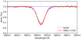
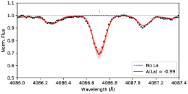
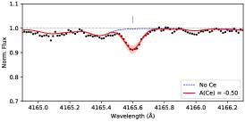
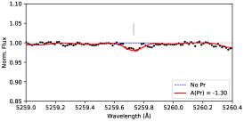
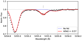
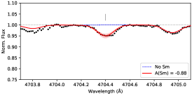
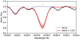
Figure 1: Portion of the spectra of the star CES0048$-$1041 around a selection of studied lines: Ba II at 5853.67 Å, La II at 4086.71 Å, Ce II at 4165.60 Å, Pr II at 5259.73 Å, Nd II at 5255.51 Å, Sm II at 4704.40 Å, and Eu II at 4129.72 Å. The black dots represent the observed spectra. The red solid lines represent the best fit, with the respective A(X) shown in the label on the lower right corner of each panel. The red shaded areas show $\pm 0.1$ dex interval around the best fit. The blue dashed lines show synthetic spectra without the studied element.

4.1 [X/Fe] versus [Fe/H]

Figure 2 shows the abundance ratios [X/Fe] as a function of the metallicity ([Fe/H]=[Fe II/H]) for our stellar sample, compared to the results obtained by François et al. (2007) and Roederer et al. (2014b). Our results are in good agreement with the literature data, and do not show any systematic offset with previous analyses. Similarly to other previous studies, we observe a large dispersion in [Ba/Fe] ratios, which increases at [Fe/H]$<$$-2.5$. For [Fe/H]$<$$-3.0$, the literature samples show a decreasing trend with metallicity, with many stars having [Ba/Fe] lower than solar yet with a fair fraction of stars having enhanced Ba (especially in carbon enhanced metal-poor stars, see Hansen et al. 2016, 2019). Our results seem to agree with this general trend, although we were only able to derive Ba abundances for two stars at these metallicities. For [La/Fe] and [Ce/Fe] abundance ratios, at lower metallicities, we observe a large spread at [Fe/H]$<$$-2.5$, similarly to the one found for [Ba/Fe], but we do not observe the same declining trend with decreasing metallicity. In our opinion, this mismatch is more likely due to an observational bias rather than to a different production site and/or mechanism as other studies show La abundance behaviour similar to that of Ba (Hansen et al. 2012). In fact, for metallicities below $-3$, it is usually only possible to derive upper limits on the abundances of La and Ce, unless the stars are enriched in these elements, while the Ba lines are strong enough to allow an actual measurement. A high dispersion is also observed for [Pr/Fe] and [Nd/Fe] at [Fe/H] $<$ $-2.5$, which increases towards lower metallicities. Similarly to La and Ce, the trend at the lowest metallicities is still not clear, as usually only upper limits can be obtained. The [Sm/Fe] and [Eu/Fe] abundance ratios behave similar to the other heavy n-capture elements, displaying an increasing scatter for metallicities below $-2.5$ dex.

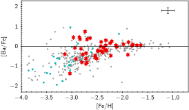
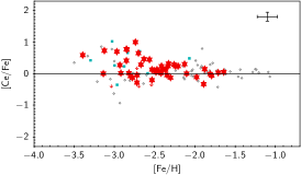
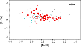
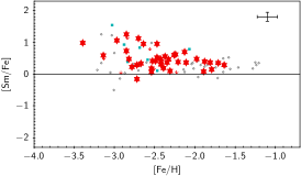
Figure 2: [Ba/Fe], [La/Fe], [Ce/Fe], [Pr/Fe], [Nd/Fe], [Sm/Fe], and [Eu/Fe] abundance ratios as a function of [Fe/H] for our sample of stars (red star symbols) compared to results obtained by François et al. 2007 (cyan squares) and Roederer et al. 2014b (grey open diamonds).

4.2 [X/H] versus [C/N]

In Paper II, we investigated the effect of extra mixing that occurs after the red giant branch (RGB) bump, which alters the surface abundances of C and N (Gratton et al. 2000), and whether it could have altered the abundance ratios of light n-capture elements, that is, Sr, Y, and Zr. The results indicate that there is no clear correlation between their abundances and [C/N] ratio, which suggests that the abundances are unaffected by mixing. In the present work, we also found no clear correlation for n-capture elements investigated here, that is, Ba, La, Ce, Pr, Nd, Sm, and Eu, as shown in Fig. C.1 in appendix C. This suggests that even these heavy elements are unaffected by the extra mixing.

4.3 NLTE corrections

Barium and europium lines are known to be sensitive to departures from LTE, also referred to as non-LTE (NLTE) effects. The NLTE effects on these lines can be strong in metal-poor stars, so it is important to understand how this effect affects the derived Ba and Eu abundances in order to investigate the nucleosynthesis of these elements. To study the NLTE effect on our derived abundances, we applied 1D NLTE corrections for Ba and Eu lines computed by L.I.Mashonkina database (Mashonkina et al. 2023). The available grids include 1D NLTE abundance corrections for five Ba II lines (4554.0298 Å, 4934.0801 Å, 5853.7002 Å, 6141.6099 Å, and 6496.8999 Å) and for 11 Eu lines (3724.9299 Å, 3819.6699 Å, 3907.1101 Å, 3930.5 Å, 3971.97 Å, 4129.7002 Å, 4205.02 Å, 4435.5801 Å, 4522.5801 Å, 6437.6401 Å, and 6645.0601 Å) in the range of stellar parameters covered by metal-poor stars. The details for the computation of NLTE corrections are described in Mashonkina & Belyaev (2019) for Ba II and Mashonkina & Gehren (2000) for Eu II.

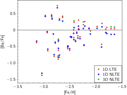
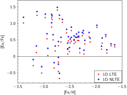
Figure 3: [Ba/Fe] and [Eu/Fe] abundance ratios as a function of [Fe/H]. Red open circles represent 1D LTE abundances. Other coloured symbols are the computed 1D NLTE (blue open diamonds) and 3D NLTE (green open squares) abundance corrections.

Figure 3 shows [Ba/Fe] and [Eu/Fe] abundance ratios as a function of [Fe/H] before and after applying NLTE corrections. The 1D NLTE corrections for Ba tend to be larger for stars with [Fe/H]$>$$-2.5$ and [Ba/Fe]$>$0 and to decrease the Ba abundances. They also seem to slightly reduce the dispersion at metallicities below $-2.5$, but the large scatter is still present. On the other hand, the 1D NLTE corrections for Eu are all positive, and on average they increase the Eu abundances by 0.13 dex. For consistency, Fe II abundances should also be corrected for NLTE effects. Contrary to Ba II and Eu II lines, the NLTE effects on Fe II lines seem to be negligible, even in very metal-poor stars (Mashonkina et al. 2011; Bergemann et al. 2012; Lind et al. 2012). Nevertheless, we checked if the NLTE effects on Fe II lines in our stars were actually negligible using the 1D NLTE corrections for Fe II lines provided by Bergemann et al. (2012). Since the NLTE corrections were available only for a sub-sample of the adopted lines, we compared the LTE Fe II abundances derived from the lines in the sub-sample to the corresponding abundances corrected for NLTE effects. We found that only for the Fe II line at 4923.932 Å the NLTE corrections are above 0.01 in all stars. It varies from +0.02 to +0.08 dex for this line, however, even when the correction is as large as +0.08, the resulting difference between the overall Fe II LTE and NLTE abundance does not exceed 0.005 dex. For this reason, Fig. 3 shows [Fe/H] in LTE.

Additionally, we investigated the three-dimensional (3D) NLTE effects on Ba lines using 3D NLTE - 1D LTE abundance corrections grids computed by Gallagher et al. (in prep). The grids are available on the ChETEC-INFRA site, which provides the details of the grid computation and the instructions on how to derive and apply the 3D NLTE corrections. Seven stars in our sample have stellar parameters inside the grid range, and the [Ba/Fe] abundances ratios corrected for 3D NLTE corrections are shown as green open squares in Fig. 3. We note that the 3D NLTE corrections are, on average, smaller than the 1D NLTE corrections and positive in sign, that is, they tend to increase Ba abundances.

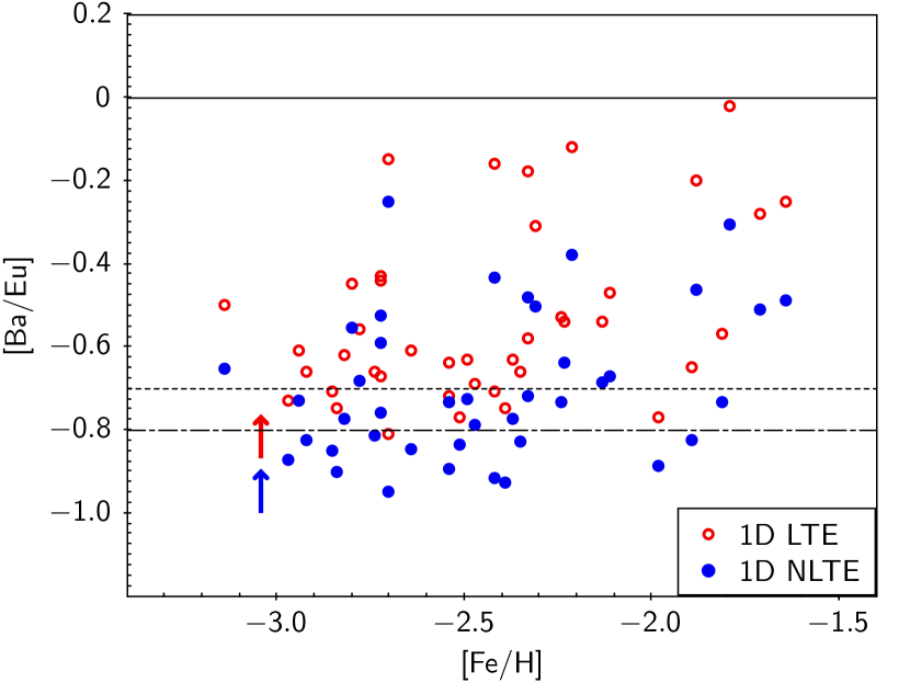
Figure 4: Comparison between 1D LTE (red open circles) and 1D NLTE (blue circles) [Ba/Eu] ratios as a function of [Fe/H] for our sample of stars. The dashed black line represent the Solar System pure $r$-process value according to Arlandini et al. 1999, while the dashed-dotted line represent the same value according to Bisterzo et al. 2014.

Mashonkina & Christlieb (2014) evaluated the empirical $r$-process log(Ba/Eu) ratio using homogeneously derived 1D NLTE abundances in a sample of very metal-poor $r$-process enhanced stars with [Eu/Fe]$>$1. In their study, the authors found that, for their sample of stars, NLTE corrections lead to lower Ba, but higher Eu abundances. This is in agreement with what we observe in our sample. They also found an average log(Ba/Eu)=0.78$\pm$0.06 in 1D NLTE for the $r$-process enhanced stars. For the six $r$-process enhanced stars with [Eu/Fe]$>$1 in our sample we find a mean log(Ba/Eu)=0.79$\pm$0.04 in 1D NLTE, which corresponds to [Ba/Eu]=$-0.87$. This result is in excellent agreement with the previous findings.

Figure 4 shows [Ba/Eu] ratios as a function of [Fe/H] in 1D LTE and 1D NLTE. In 1D LTE, 16 out of 43 stars have [Ba/Eu]$\leq$$-0.7$ within uncertainties, where [Ba/Eu]=$-0.7$ is the Solar System pure $r$-process value according to Arlandini et al. (1999, hereafter A99). If we instead take [Ba/Eu]=$-0.8$ as the Solar System pure $r$-process value (Bisterzo et al. 2014, hereafter B14), we note that the number of stars compatible with solar pure $r$-process [Ba/Eu] is reduced to 7 out of 43. When the 1D NLTE corrections are applied, we see that 30 out of 43 stars have [Ba/Eu]$\leq$$-$0.7 within errors, and 24 have also [Ba/Eu]$\leq$$-$0.8. Since the 1D NLTE corrections are available only for Ba and Eu, the results presented in this study are 1D LTE abundances. As a reference for the contributions of $s$- and $r$- processes in the Solar System, we refer to the values presented in Arlandini et al. (1999).

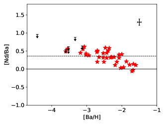
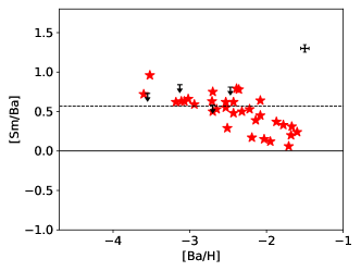
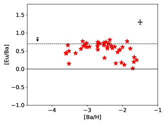
Figure 5: [La/Ba], [Nd/Ba], [Sm/Ba] and [Eu/Ba] as a function of [Ba/H] for our sample of stars. The black arrows represent upper limits of abundance ratios. A representative error bar is shown in the upper-right corner of each panel. The dashed black lines represent the Solar System pure $r$-process values according to Arlandini et al. (1999).

5 Discussion

5.1 $s$-process versus $r$-process

The observed increasing scatter of [Ba/Fe] ratios towards low metallicities shown in Fig. 2 is thought to be caused by a variation of the Ba nucleosynthesis at [Fe/H] $\approx$ $-2.5$ and below (see e.g. Gratton & Sneden 1994; McWilliam 1998; Burris et al. 2000; Honda et al. 2004; Simmerer et al. 2004; François et al. 2007; Hansen et al. 2012). At later times and higher metallicities, the $s$-process elements such as Ba are dominantly produced by low- and intermediate-mass AGB stars (see e.g. Busso et al. 1999; Käppeler et al. 2011; Karakas & Lattanzio 2014). However, in the early Galaxy, AGB stars did not have time to significantly enrich the interstellar medium given their long lifetimes. Fast-rotating massive stars (FRMS) are expected to be a source of $s$-process at this epoch, but their contribution to the nucleosynthesis of elements around (and heavier than) Ba is predicted to be overall small (see e.g. Frischknecht et al. 2016). Therefore, at metallicities below $\sim$$-2.5$, the $r$-process is more likely the primary production mechanism of Ba. Similarly to Ba ($s$-process: 81%, A99), most La and Ce in the Solar neighbourhood were produced by the $s$-process (62% and 77%, A99), while Pr and Nd were more equally produced by the $s$- and $r$-processes ($s$-process: 49% and 56%, A99). It is therefore likely that the production of all those elements at low metallicities occurs also predominantly through the $r$-process.

Figures 5 and C.2-C.6 in appendix C show the correlations between heavy elements pairs ([element1/element2] versus [element2/H]) for our sample of stars. In Fig. 5, [La/Ba], [Nd/Ba], [Sm/Ba], and [Eu/Ba] as a function of [Ba/H] are shown. We note that in each plot, for values of [Ba/H]$\approx$$-2.5$, there is a change in the trends: for [Ba/H]$\gtrsim$$-2.5$ the scatter in the abundance ratios increases, and a decreasing trend seems to appear as [Ba/H] increases. For [Ba/H]$\lesssim$$-2.5$, the observed trend is generally flat, and the stars tend to clump around the Solar System pure $r$-process value computed by A99. To estimate at which values of [Ba/H] and [Fe/H] the possible onset of the $s$-process occurs in the chemistry of our sample stars, we applied a mean shift clustering algorithm with a flat kernel using the Python module Scikit-learn (Comaniciu & Meer 2002; Pedregosa et al. 2011). Mean shift clustering is a non-parametric, density-based clustering algorithm that can be used to identify clusters in a data set. Given a set of data points, the algorithm shifts each data point towards the maximum increase in the density of points within a certain radius. The operation is iterated until the points converge to a local maximum of the density function, which correspond to the cluster centroid. The main advantages of the mean shift clustering algorithm are that it does not require the number of clusters to be specified in advance and can handle arbitrary shapes and sizes of clusters.

We applied the mean shift clustering to [Eu/Ba] abundance ratios as a function of [Ba/H] and identified three clusters as shown in Fig. 6. We calculated the mean, median, and standard deviation of [Ba/H] and [Fe/H] for the stars belonging to the cluster that corresponds to the transition region between the region with [Eu/Ba]$\sim$constant and the region with a large dispersion in [Eu/Ba] (blue cluster in Fig. 6). We then repeated the procedure for [La/Ba], [Nd/Ba], and [Sm/Ba] ratios as a function of [Ba/H] to check if the values were different adopting different abundance ratios. The results are listed in Table 3. The median of the median values we obtained for [Fe/H] is $-2.42$ ($\sigma$=0.02) and for [Ba/H] is $-2.42$ ($\sigma$=0.04). These results suggest that the change in the trend happens at [Ba/H]=$-2.4$, which corresponds to a metallicity of [Fe/H]=$-2.4$. For [Ba/H]$<$$-2.4$, the flat trend and the clustering around the solar pure $r$-process values support the scenario of the $r$-process as the primary production mechanism of Ba (and other heavy n-capture elements) at low metallicities. On the other hand, the larger scatter observed for [Ba/H]$>$$-2.4$ can be interpreted as the onset of the $s$-process contribution in Ba nucleosynthesis.

Our results are in line with previous studies of neutron capture elements in the early Galaxy. Burris et al. (2000), in the context of the Bond survey, found the presence of $s$-nuclei of Ba already in stars with a metallicity of about $-2.7$, but inferred finally that the bulk of the $s$-processing was delayed until [Fe/H] $\simeq-2.2$. From analysis of the [La/Eu] ratios, Simmerer et al. (2004) concluded that the $s$-process may be active as early as [Fe/H]=$-2.6$. Hansen et al. (2012) suggested that the contribution of the $s$-process might start at [Fe/H]=$-2.5$, given the change in the observed abundance trends of [Sr/Fe], [Y/Fe], [Zr/Fe], and [Ba/Fe] as a function of [Fe/H].

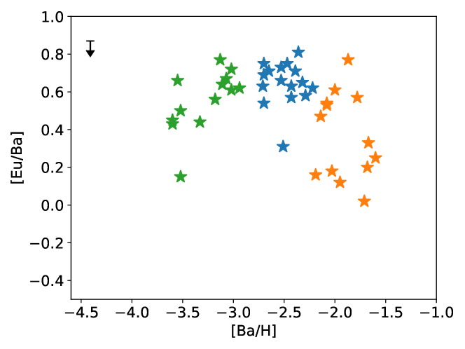
Figure 6: [Eu/Ba] as a function of [Ba/H] for our sample of stars after applying the mean shift clustering algorithm. The three clusters found by the algorithm are visible in different colours. The star CES1237+1922 is represented by a black arrow (upper limit), and it was not considered when applying the clustering algorithm.

Table 3: Mean, median and standard deviations for [Fe/H] and [Ba/H].

[X/Ba]	Mean[Fe/H]	Median[Fe/H]	$\sigma_{\rm[Fe/H]}$	Mean[Ba/H]	Median[Ba/H]	$\sigma_{\rm[Ba/H]}$
La	$-$2.52	$-$2.43	0.32	$-$2.41	$-$2.43	0.10
Nd	$-$2.48	$-$2.40	0.32	$-$2.38	$-$2.41	0.14
Sm	$-$2.46	$-$2.40	0.33	$-$2.38	$-$2.41	0.14
Eu	$-$2.48	$-$2.43	0.27	$-$2.50	$-$2.49	0.16

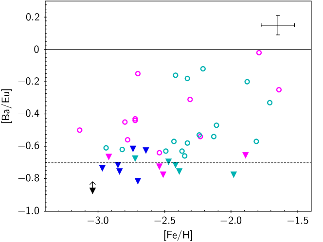
Figure 7: [Ba/Eu] abundance ratios as a function of [Fe/H]. Filled triangles are stars compatible within uncertainties with [Ba/Eu]$\leq$$-0.7$ (Solar System pure $r$-process according to A99). Open circles are stars with [Ba/Eu]$>$$-0.7$. Symbols are colour coded according to the Christlieb et al. (2004) classification for $r$-process enhanced stars. Blue, cyan, and magenta symbols represent $r$-II, $r$-I, and $r$-poor stars respectively. The black triangle indicates the star CES1237+1922.

Figure 7 shows [Ba/Eu] abundance ratios as a function of [Fe/H] for our sample of stars. We see that all the 43 stars with both Ba and Eu measurements in our sample have [Ba/Eu]$<$0. At these low [Fe/H], we expect the majority of stars to have [Ba/Eu]$<$0, because the $r$-process is the dominant process in the heavy elements’ nucleosynthesis. Following the classification from Christlieb et al. (2004), 27 are $r$-process-rich stars ($r$-rich; [Eu/Fe]$\geq$0.3), of which six are $r$-II stars ([Eu/Fe]$>$1), and 21 are $r$-I stars (0.3$\leq$[Eu/Fe]$\leq$1.0). The remaining 16 stars have [Eu/Fe]$<$0.3, and we shall refer to them as $r$-process-poor or $r$-poor stars. In our sample, 16 out of 43 stars are compatible with [Ba/Eu]$\leq$$-0.7$ within uncertainties ($r$-pure), which is the Solar System pure $r$-process value from A99. We note that all the $r$-II stars are compatible within errors with the Solar System pure $r$-process value. Among the $r$-I stars, only five out of 21 are compatible with the $r$-pure value. It is interesting to notice that also five $r$-poor stars ([Eu/Fe]$<$0.3) are compatible with the $r$-pure value. Figure 7 also seems to indicate that stars with [Ba/Eu] ratios consistent with the $r$-pure value are found at metallicities at least as high as [Fe/H]=$-1.9$.

To understand if the stars compatible with $r$-pure [Ba/Eu] follow some trends or show a common behaviour, we checked for possible correlations between Ba and Eu with other elements. Mg is mainly produced in massive stars and released into the interstellar medium by core collapse supernovae (CC SNe or SNe II), contrary to Fe which can also be produced in SNe type Ia. For this reason, Mg has been suggested as an alternative ‘reference element’ to Fe when investigating the Galactic chemical evolution (see e.g. Cayrel et al. 2004; Mashonkina et al. 2017b). Figure 8 shows [Ba/Mg] and [Eu/Mg] as a function of [Mg/H] for our sample of stars. Similarly to Fig. 2, the general trends of [Ba/Mg] and [Eu/Mg] seem to change at [Mg/H]$\sim$$-2.2$: for [Mg/H]$>$$-2.2$, [Ba/Mg] and [Eu/Mg] abundance ratios follow a flat trend, with an average of [Ba/Mg]=$-0.42$ ($\sigma$=0.26) and [Eu/Mg]=0.08 ($\sigma$=0.21) respectively, while for [Mg/H]$<$$-2.2$ the abundance ratios show a large scatter, with values spanning over 2 dex. We note that in the [Ba/Mg] versus [Mg/H] plot, the $r$-II stars stand out from the overall decreasing trend of the other stars, showing [Ba/Mg]$\gtrsim$0 abundance ratios. The same is visible in the [Ba/Fe] versus [Fe/H] plot in Fig. 2. We also note that the $r$-pure stars do not show any particular trend compared to the other stars in the sample when comparing to Mg.

The wide dispersion observed at [Mg/H]$<$$-2.2$ for both Ba and Eu seems to suggest that these elements are not co-produced with Mg, implying that normal SNe II are unlikely to be the main or dominant formation sites of Ba and Eu. This scenario is supported by nucleosynthesis models, which show that classic CC SNe would only be able to produce elements lighter than Ba (see e.g. Hansen et al. 2014; Arcones & Thielemann 2023, and references therein). However, some special (and rare) classes of SNe, such as MRD SNe, depending on the explosion dynamics, may produce heavy elements through the $r$-process, thus being able to explain the large dispersion observed at low metallicities (see e.g. Winteler et al. 2012; Nishimura et al. 2015, 2017; Mösta et al. 2018; Halevi & Mösta 2018; Reichert et al. 2021, 2023, 2024). For this reason, MRD SNe together with NSMs, are considered to be some of the main sources of $r$-process at low metallicities (see e.g. Cowan et al. 2021). All yields contribute to the next generation of stars via mixing processes in the ISM. To find the best tracers, mono-enrichment is desired (see e.g. Magg et al. 2020; Hansen et al. 2020) so further conclusions would require mono-enriched stars as well as more complete abundance patterns.

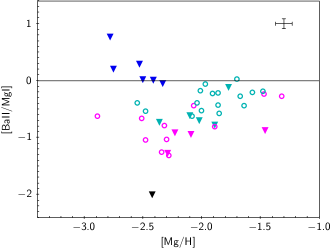
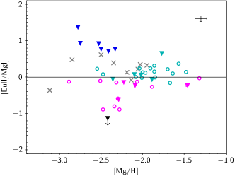
Figure 8: [Ba/Mg] and [Eu/Mg] abundance ratios as a function of [Mg/H]. Coloured symbols as in Fig. 7. Grey crosses represent stars without Ba abundance measurement. The black triangle indicates the star CES1237+1922.

5.2 Light versus heavy n-capture elements

Light n-capture elements, such as Sr, are produced in different ways as a function of metallicity, but mainly by the $s$-process in the solar inventory (85%, A99). Previous studies of metal-poor stars in the Milky Way pointed out that the large scatter observed in [Sr/Ba] at low [Ba/Fe] suggests the presence of an additional process to the main $r$-, that produce light n-capture elements (for example, Sr, Y, Zr) but not the heavy ones, such as Ba (Travaglio et al. 2004; Honda et al. 2004; François et al. 2007; Qian & Wasserburg 2008; Andrievsky et al. 2011; Hansen et al. 2012; Roederer 2013; Yong et al. 2013; Hansen et al. 2014; Spite et al. 2014, 2018; Han et al. 2021). The nucleosynthesis processes and astrophysical sites associated with the production of light n-capture elements are still a matter of debate, as several processes could be involved (see e.g. the review by Arcones & Thielemann 2023). As discussed in Paper I, neutrino-driven winds in CC SNe could be a possible formation site for light n-capture elements. In these environments, if the conditions are mildly neutron-rich, elements up to Z$\sim$50 can be produced by the weak $r$-process (weak-$r$; see e.g. Arcones & Bliss 2014), whereas if the conditions are proton-rich, these nuclei can also be produced by the $\nu$p-process (see e.g. Wanajo 2006; Fröhlich et al. 2006; Pruet et al. 2006). Both processes are able to produce abundance patterns compatible with the ones observed for light n-capture elements in metal-poor stars (Arcones & Montes 2011), therefore the observationally derived abundances could be produced by the weak $r$-process, the $\nu$p-process, a main r-process or a combination of those (see e.g. Hansen et al. 2014, and references therein). The FRMS could also be a possible formation site for light n-capture elements, as they are thought to be a source of $s$-process elements through rotation-induced mixing, and they are expected to produce heavy elements up to Ba (‘weak $s$-process’; see e.g. Pignatari et al. 2008; Frischknecht et al. 2012, 2016; Limongi & Chieffi 2018). Another possible process involved in the production of light n-capture elements at low metallicities is the lighter element primary process (LEPP, Travaglio et al. 2004; Montes et al. 2007).

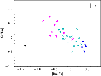
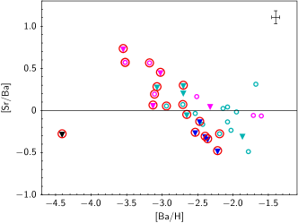
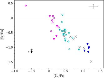
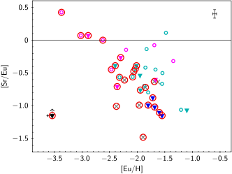
Figure 9: [Sr/Ba] as a function of [Ba/Fe] (upper left panel) and [Ba/H] (upper right panel), and [Sr/Eu] as a function of [Eu/Fe] (lower left panel) and [Eu/H] (lower right panel) for our sample of stars. Coloured symbols as in Fig. 7 and Fig. 8. Red open circles highlight stars with [Fe/H]$<$$-2.4$.

Figure 9 shows [Sr/Ba] as a function of [Ba/Fe] (upper left panel) and [Sr/Eu] as a function of [Eu/Fe] (lower left panel) for our sample of stars. In our sample we do not see the large scatter in [Sr/Ba] observed in previous studies, for example in Spite et al. (2018), with the exception of the star CES1237+1922 (black triangle in Fig. 9). However, looking at Figure 4 of Spite et al. (2018), we see that the scatter in [Sr/Ba] increases for [Ba/Fe]$\lesssim$$-0.5$. In our sample, only five stars with both Sr and Ba measurements have [Ba/Fe]$\lesssim$$-0.5$, and indeed the [Sr/Ba] for these stars vary from $-0.28$ (CES1237+1922) to $+0.73$ (CES2019-6130). We observe that, for all stars except CES1237+1922, [Sr/Ba] (and [Sr/Eu]) increases when [Ba/Fe] (and [Eu/Fe]) decreases. We also note that $r$-II stars have on average [Sr/Ba]$\sim$$-0.3$, which is close to the empirical $r$-process ratio [Sr/Ba]=$-0.4$ observed in strongly enhanced $r$-rich stars (see e.g. Barklem et al. 2005; Mashonkina et al. 2017b).

When comparing [Sr/Ba] to [Ba/H] (upper right panel of Fig. 9) and [Sr/Eu] to [Eu/H] (lower right panel of Fig. 9) abundance ratios, the decreasing trend is still visible, with an increasing scatter towards the highest [Ba/H] and [Eu/H] abundances. If we remove the stars with [Fe/H]$>$–2.4, the downward trend is very clean, and the scatter is drastically reduced (stars identified by red open circles in Fig. 9). This is likely due to the fact that stars with [Fe/H]$>$–2.4 can already show contamination from other processes, such as the $s$-process, in Ba and Sr nucleosynthesis, therefore the scatter increases (see e.g. Hansen & Primas 2011; Hansen et al. 2012, 2014). The $r$-pure stars seem to show a scatter as well, and to behave similar to the other stars in the sample. This behaviour seems to indicate that $r$-pure stars need not to be produced through different formation channels and/or scenarios.

According to Spite et al. (2018), at a given [Ba/Fe], the star’s [Sr/Ba] ratio depends on how strong the contribution is from the process that produces only light n-capture elements. This scenario implies that stars such as CES2019-6130 ([Ba/Fe]=$-0.63$, [Sr/Ba]=$+0.73$) are likely formed in a gas polluted by both mechanisms, but the contribution from the light n-capture component is dominating, while n-capture rich stars might be formed in a gas polluted by both mechanisms as well, but the contribution from the main $r$-process is so large that the contribution from light n-capture component would not alter the abundance pattern. Our results seem to support this scenario, although it is difficult to distinguish whether the two processes are independent, and thus generated in different astrophysical scenarios, or whether they reflect varying conditions in the micro physics of the same formation site (see Arcones & Thielemann 2023, and references therein).

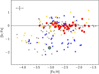
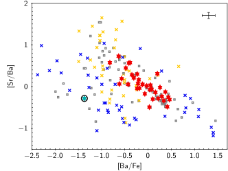
Figure 10: [Sr/Fe] as a function of [Fe/H] (upper panel) and [Sr/Ba] as a function of [Ba/Fe] abundance ratios (lower panel) for our sample of stars (red star symbols). The cyan star with a black open circle indicates the star CES1237+1922. Grey open squares are stars in the Milky Way halo and crosses are stars in dSph (yellow) and UFD galaxies (blue) in the literature. Literature abundance ratios are taken from: François et al. 2007 (Milky Way halo), Norris et al. 2010 (Bootes I), Frebel et al. 2010 (Ursa Major II, Coma Berenices), Simon et al. 2010 (Leo IV), Hansen et al. 2012 (Milky Way halo), Ishigaki et al. 2014 (Bootes I), François et al. 2016 (Canes Venatici I, Hercules), Ji et al. 2016 (Reticulum II), Roederer et al. 2016 (Reticulum II), Mashonkina et al. 2017b (Milky Way halo, Sculptor, Fornax, Sextans, Ursa Minor, Bootes I, Ursa Major II, Leo IV), Reichert et al. 2020 (Draco, Sculptor, Ursa Minor, Sextans, Sagittarius, Fornax, Ursa Major II, Bootes I, Segue 1, Triangulum II), Sitnova et al. 2021 (Segue 1, Triangulum II, Coma Berenices, Ursa Major II), and Skúladóttir et al. 2024 (Sculptor) .

5.3 The peculiar star CES1237+1922

In Paper I, we found that CES1237+1922 (also known as BS 16085-0050) is deficient in Sr, Y, and Zr compared to the other stars in our sample. In Fig. 9, we see that the star does not seem to follow the general trend observed for the rest of the stars in the sample. Figure 10 shows [Sr/Fe] versus [Fe/H] and [Sr/Ba] versus [Ba/Fe] abundance ratios for our sample of stars and the ones observed in the Milky Way halo, dwarf Spheroidal (dSph), and Ultra-faint Dwarf (UFD) galaxies. The literature values for UFD galaxies were collected using the JINAbase database. Stars in UFD galaxies show a large scatter in [Sr/Fe], as shown in the upper panel of Fig. 10, overlapping with both MW and dSph stars. With the exception of stars in Canes Venatici I and Reticulum II, which are enhanced in n-capture elements, the other stars in UFDs show [Sr/Fe]$\lesssim$–0.6, while Milky Way halo stars with similar low [Sr/Fe] become more frequent for [Fe/H]$\lesssim$–3 (see e.g. Frebel et al. 2010; Simon et al. 2010; Koch et al. 2013; François et al. 2016; Roederer et al. 2016; Ji et al. 2016; Mashonkina et al. 2017b; Sitnova et al. 2021). The enrichment history of such stars is still not clear yet, since for most of these extremely metal-poor stars only upper limits can usually be measured for most of the n-capture elements, with Sr and Ba being an exception due to their strong lines (see e.g. Roederer 2013; Hansen et al. 2013; Spite et al. 2018).

In the lower panel of Fig. 10, we note that other halo stars similar to CES1237+1922 exist in the literature, and are characterised by [Fe/H]$\lesssim$–3, [Sr/Fe]$<$–1.5, and [Ba/Fe]$<$–1. Since these stars lie in the region of the [Sr/Ba] versus [Ba/Fe] diagram mainly occupied by UFD stars, it has been suggested that halo stars such as CES1237+1922 could be formed in UFDs that were later accreted by the Milky Way (see Andales et al. 2024, and references therein). However, it is also possible that these stars formed in the Milky Way through the same mechanism that is producing low [Sr/Ba] stars in UFDs. We defer further discussion on our low [Sr/Ba] star to Lombardo et al. (in prep).

5.4 Comparison with Galactic chemical evolution models

In Figs. 11 and 12, we compare our measured abundance ratios to the ones predicted by the GCE models from Cescutti & Chiappini (2014), Cescutti et al. (2015) and Rizzuti et al. (2021). These models consider the stochastic formation of stars and $r$-process events, a concept described in Cescutti (2008). The results show the dispersion created by different nucleosynthesis sites and at the same time reproduce the main trend of chemical evolution of the stellar system considered. To recover the possible combinations of enrichments, we assume several isolated volumes ($>$100), each of them containing the typical mass of gas swept by a SNe II explosion, the minimum mass that we can consider isolated. We recall that the chemical evolution models are not ab initio modelling, therefore parameters such as infall, outflow of gas, and star formation efficiency should be tuned to reproduce the observed quantities of the stellar system we intend to reproduce.

In Cescutti & Chiappini (2014), the stellar system analysed was at the more metal-poor tail of the Galactic halo. Concerning nucleosynthesis, the model assumed three main sources for the neutron capture elements. The main $s$-process is produced by low-mass AGB stars with the yields of the F.R.U.I.T.Y. database (Cristallo et al. 2011). The $r$-process site is MRD SNe and the model considers 10% of all the exploding SNe II to enrich the interstellar medium with $r$-process material. The mean yields for Ba are $8.0\times 10^{-6}$ $\rm M_{\odot}$ (obtained from fine-tuning the model of Cescutti et al. 2013), and they also consider a possible variation in the ejecta of the single event (for details see Cescutti & Chiappini 2014). The other chemical elements (for example Eu) are simply scaled using the Solar System $r$-process contribution as determined by Simmerer et al. (2004). Finally, they also assume the production of $s$-process from massive stars, thanks to FRMS considered in Frischknecht et al. (2016), with fixed rotation velocity. These yields can produce $s$-process elements up to the second peak (barium and lanthanum).

On the other hand, Cescutti et al. (2015) assumed the same sources for $s$-process, but investigated a different scenario for $r$-process, namely a contribution from MRD SNe, NSMs or both. They found that the synthesis of Eu in the Galaxy can be explained by either only NSMs with a short time delay of 1 Myr, or both MRD SNe and NSMs assuming a fixed delay of 100 Myr, with similar results. This is in agreement with the results from Matteucci et al. (2014), who found that NSMs can be the sole responsible of $r$-process enrichment only if they have a very short time-scale.

Rizzuti et al. (2021) focused instead on $s$-process sources, having fixed the $r$-process to NSMs with 1 Myr time delay. They have employed the FRMS from Limongi & Chieffi (2018) for low-metallicity $s$-process, and calibrated the rotation velocity distribution in order to reproduce at best the dispersion in Sr and Ba. They showed that these assumptions can also explain the chemical evolution of Y, Zr, and La, despite the fact that these have not been used for calibration.

The models run with different $r$-process sources show that, apart from an offset, the observed trends for [Ba/Fe] and [Eu/Fe] can be reproduced by all models, validating both scenarios with MRD SNe and/or NSMs (see Fig. 11 and C.7 in appendix C). At the lowest metallicity, elements such as Sr may receive a contribution from the FRMS that contribute to the early star-to-star scatter of these elements (typically up to the second peak). FRMS also contribute to the large variation in [Sr/Ba] from $-0.5$ to $+1.0$ at very low [Ba/Fe] (see Fig. 12, left panel). Finally, FRMS may also explain part of the observed spread in [Ba/Eu] at low metallicity, shown in the right panel of Fig. 12. In the same figure, the contribution from AGB stars is also visible, where they produce the sharp increase in [Ba/Eu] ratio at [Fe/H]$>$$-1.0$. In the [Ba/Fe] versus [Fe/H] plot (Fig. 11), their enrichment is neutralised by the iron produced by SNe Ia with similar timescales. The predictions of the GCE model for [Fe/H]$>$$-1.5$ are less reliable, because the model has been created to explain the most metal-poor part of the halo, and has not been calibrated yet for this metallicity range. It is possible that the contribution of $s$-process from FRMS also extends above $-1.5$, while in Rizzuti et al. (2021) stars stop rotating at higher metallicity and therefore create the visible plateau, or that the AGB contribution begins at lower metallicities. Overall, the GCE models show that the observational data provide an excellent constraint to the neutron capture nucleosynthesis sites, showing that the strong $r$-process contribution dominates the lowest metallicity, but also the need for additional production sites, such as FRMS investigated here, to reproduce the dispersion observed in heavy element ratios.

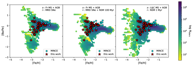
Figure 11: [Ba/Fe] abundance ratios as a function of [Fe/H] for our sample of stars (red stars) and MINCE data (François et al. 2024, cyan squares) compared to GCE models. Left panel: GCE model from Cescutti & Chiappini (2014). Centre panel: GCE model from Cescutti et al. (2015). Right panel: GCE model from Rizzuti et al. (2021) (see text for more details).

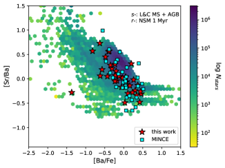
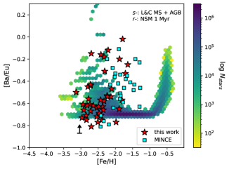
Figure 12: [Sr/Ba] (left) and [Ba/Eu] (right) abundance ratios as a function of [Ba/Fe] and [Fe/H], respectively, for our sample of stars (red stars) and MINCE data (François et al. 2024, cyan squares) compared to the GCE model of Rizzuti et al. (2021).

6 Conclusions

In this study we present the chemical abundances of the heavy n-capture elements from Ba to Eu for the CERES sample, adopting the stellar parameters and the abundances of light elements derived in Paper I and II. The main conclusions of this study are the following:

• We derived abundances or upper limits of Ba, La, Ce, Pr, Nd, Sm, and Eu for a sample of 52 Milky Way halo stars. The general trends observed for heavy n-capture element abundance ratios ([X/Fe]) as a function of [Fe/H] are in good agreement with the ones found in previous studies.

• We applied 1D NLTE corrections to Ba and Eu abundances. We found that the corrections for Ba tend to be larger for stars with [Fe/H]$>$–2.5 and [Ba/Fe]$>$0, and to decrease the Ba abundances. We also applied 3D NLTE corrections for seven stars in our sample, and found that they are on average smaller than 1D NLTE corrections and positive in sign, thus increasing the Ba abundances. We found that 1D NLTE corrections for Eu are all positive in sign and increase the Eu abundances. This is in agreement with previous studies.

• We estimated at which values of [Ba/H] and [Fe/H] the onset of the $s$-process occurs in our sample of stars using the mean shift clustering algorithm. We found that the change in the trend happens at [Ba/H]=$-2.4$, which corresponds to a metallicity of [Fe/H]=$-2.4$. This suggests that, for [Ba/H]$<$$-2.4$, the $r$-process is likely the primary production mechanism of Ba, and the large scatter observed at [Ba/H]$>$$-2.4$ is probably due to the onset of the $s$-process in Ba nucleosynthesis suffering from time delay in the Milky Way halo.

• We selected stars with [Ba/Eu] compatible with the Solar System pure $r$-process values ($r$-pure), to check for possible correlations with other elements. The $r$-pure stars did not show any particular trend compared to the others in the sample. This seems to suggest that $r$-pure stars might be produced through similar formation channels and/or scenarios similar to stars with other $r$-process enrichments.

• The star CES1237+1922 does not follow the general trend observed for other stars in the sample, and it is characterised by very low n-capture elements abundances. Other stars in the literature show a similar chemistry, and they lie in the region of the [Sr/Ba] versus [Ba/Fe] diagram mainly occupied by UFD stars. The origin of such stars is still uncertain, as they could form in situ or UFD galaxies and later be accreted by the Milky Way.

• The comparison of the abundances obtained in this study to up-to-date Galactic Chemical Evolution models show the crucial role of $r$-process sources at low metallicities, whether they are NSMs or MRD SNe, to explain the measured abundances of heavy elements. The large scatter in the abundance ratios between elements produced by $s$- and $r$-processes seems to suggest that other sources may contribute at these low metallicities, one of which could be FRMS.

7 Data availability

Table 1 is only available in electronic form at the CDS via anonymous ftp to cdsarc.u-strasbg.fr (130.79.128.5) or via http://cdsweb.u-strasbg.fr/cgi-bin/qcat?J/A+A/. Appendix A and C are only available in electronic form at https://doi.org/10.5281/zenodo.14218032.

Appendix A Additional tables

Table 4: Stellar parameters for our sample stars as derived in Paper I.

Star	$\mathrm{T_{eff}}$	$\mathrm{\log g}$	$\mathrm{v_{turb}}$	[Fe$/$H]
	K	dex	$\mathrm{km\,s^{-1}}$	dex
CES0031–1647	4960	1.83	1.91	$-$2.49
CES0045–0932	5023	2.29	1.76	$-$2.95
CES0048–1041	4856	1.68	1.93	$-$2.48
CES0055–3345	5056	2.45	1.66	$-$2.36
CES0059–4524	5129	2.72	1.56	$-$2.39
CES0102–6143	5083	2.37	1.75	$-$2.86
CES0107–6125	5286	2.97	1.54	$-$2.59
CES0109–0443	5206	2.74	1.69	$-$3.23
CES0215–2554	5077	2.00	1.91	$-$2.73
CES0221–2130	4908	1.84	1.84	$-$1.99
CES0242–0754	4713	1.36	2.03	$-$2.90
CES0301+0616	5224	3.01	1.51	$-$2.93
CES0338–2402	5244	2.78	1.62	$-$2.81
CES0413+0636	4512	1.10	2.01	$-$2.24
CES0419–3651	5092	2.29	1.78	$-$2.81
CES0422–3715	5104	2.46	1.68	$-$2.45
CES0424–1501	4646	1.74	1.74	$-$1.79
CES0430–1334	5636	3.07	1.63	$-$2.09
CES0444–1228	4575	1.40	1.92	$-$2.54
CES0518–3817	5291	3.06	1.49	$-$2.49
CES0527–2052	4772	1.81	1.84	$-$2.75
CES0547–1739	4345	0.90	2.01	$-$2.05
CES0747–0405	4111	0.54	2.08	$-$2.25
CES0900–6222	4329	0.94	1.98	$-$2.11
CES0908–6607	4489	0.90	2.12	$-$2.62
CES0919–6958	4430	0.70	2.17	$-$2.46
CES1116–7250	4106	0.48	2.14	$-$2.74
CES1221–0328	5145	2.76	1.60	$-$2.96
CES1222+1136	4832	1.72	1.93	$-$2.91
CES1226+0518	5341	2.84	1.60	$-$2.38
CES1228+1220	5089	2.04	1.87	$-$2.32
CES1237+1922	4960	1.86	1.95	$-$3.19
CES1245–2425	5023	2.35	1.72	$-$2.85
CES1322–1355	4960	1.81	1.96	$-$2.93
CES1402+0941	4682	1.35	2.01	$-$2.79
CES1405–1451	4642	1.58	1.81	$-$1.87
CES1413–7609	4782	1.72	1.87	$-$2.52
CES1427–2214	4913	1.99	1.85	$-$3.05
CES1436–2906	5280	3.15	1.42	$-$2.15
CES1543+0201	5157	2.77	1.57	$-$2.65
CES1552+0517	5013	2.30	1.72	$-$2.60
CES1732+2344	5370	2.82	1.65	$-$2.57
CES1804+0346	4390	0.80	2.12	$-$2.48
CES1942–6103	4748	1.53	2.01	$-$3.34
CES2019–6130	4590	1.13	2.09	$-$2.97
CES2103–6505	4916	2.05	1.85	$-$3.58
CES2231–3238	5222	2.67	1.67	$-$2.77
CES2232–4138	5194	2.76	1.59	$-$2.58
CES2250–4057	5634	2.51	1.88	$-$2.14
CES2254–4209	4805	1.98	1.79	$-$2.88
CES2330–5626	5028	2.31	1.75	$-$3.10
CES2334–2642	4640	1.42	2.02	$-$3.48

Table 5: List of atomic data without hyperfine and isotopic structure.

Element	Wavelength (Å)	$\chi_{exc}$	$\log gf$
	Å
Ba II	5853.668	0.604	–1.01
Ba II	6141.713	0.703	–0.08
Ba II	6496.897	0.604	–0.38
La II	3949.100	0.403	0.49
La II	4086.710	0.000	–0.07
La II	4123.220	0.321	0.13
La II	4920.980	0.126	–0.58
Ce II	3577.456	0.470	0.14
Ce II	3999.237	0.295	0.06
Ce II	4073.474	0.477	0.21
Ce II	4083.222	0.700	0.27
Ce II	4118.143	0.696	0.13
Ce II	4120.827	0.320	–0.37
Ce II	4137.645	0.516	0.40
Ce II	4165.599	0.909	0.52
Ce II	5274.229	1.044	0.13
Pr II	4408.810	0.000	0.05
Pr II	5259.731	0.633	0.12
Pr II	5322.770	0.482	–0.12
Nd II	3784.240	0.380	0.15
Nd II	3826.410	0.064	–0.41
Nd II	4021.330	0.320	–0.10
Nd II	4446.380	0.204	–0.35
Nd II	4959.120	0.064	–0.80
Nd II	5255.510	0.204	–0.67
Nd II	5293.160	0.822	0.10
Nd II	5319.810	0.550	–0.14
Sm II	4434.320	0.378	–0.07
Sm II	4704.400	0.000	–0.86
Eu II	3819.670	0.000	0.51
Eu II	4129.720	0.000	0.22
Eu II	6645.060	1.379	0.12

Table 6: Hyperfine and isotopic structure for Ba II lines (Z=56).

Wavelength	Isotope	$\chi_{exc}$	$\log gf$
Å
5853.686	137	0.604	–2.066
5853.687	135	0.604	–2.066
5853.687	137	0.604	–2.009
5853.688	135	0.604	–2.009
5853.689	135	0.604	–2.215
5853.689	137	0.604	–2.215
5853.690	134	0.604	–1.010
5853.690	135	0.604	–2.620
5853.690	135	0.604	–1.914
5853.690	135	0.604	–1.466
5853.690	136	0.604	–1.010
5853.690	137	0.604	–2.620
5853.690	137	0.604	–1.914
5853.690	137	0.604	–1.466
5853.690	138	0.604	–1.010
5853.691	135	0.604	–2.215
5853.692	137	0.604	–2.215
5853.693	135	0.604	–2.009
5853.693	137	0.604	–2.009
5853.694	135	0.604	–2.066
5853.694	137	0.604	–2.066
6141.725	135	0.704	–2.456
6141.725	137	0.704	–2.456
6141.727	135	0.704	–1.311
6141.727	137	0.704	–1.311
6141.728	135	0.704	–2.284
6141.728	137	0.704	–2.284
6141.729	135	0.704	–1.214
6141.729	135	0.704	–0.503
6141.729	137	0.704	–1.214
6141.729	137	0.704	–0.503
6141.730	134	0.704	–0.077
6141.730	136	0.704	–0.077
6141.730	138	0.704	–0.077
6141.731	135	0.704	–1.327
6141.731	135	0.704	–0.709
6141.731	137	0.704	–1.327
6141.731	137	0.704	–0.709
6141.732	135	0.704	–1.281
6141.732	135	0.704	–0.959
6141.732	137	0.704	–0.959
6141.733	137	0.704	–1.281
6496.898	137	0.604	–1.886
6496.899	135	0.604	–1.886
6496.901	137	0.604	–1.186
6496.902	135	0.604	–1.186
6496.906	135	0.604	–0.739
6496.906	137	0.604	–0.739
6496.910	134	0.604	–0.380
6496.910	136	0.604	–0.380
6496.910	138	0.604	–0.380
6496.916	135	0.604	–1.583
6496.916	137	0.604	–1.583
6496.917	135	0.604	–1.186
6496.918	137	0.604	–1.186
6496.920	135	0.604	–1.186
6496.922	137	0.604	–1.186

Table 7: Hyperfine and isotopic structure for La II lines (Z=57).

Wavelength	Isotope	$\chi_{exc}$	$\log gf$
Å
3949.0377	139	0.403	–1.337
3949.0387	139	0.403	–1.191
3949.0444	139	0.403	–0.995
3949.0460	139	0.403	–1.008
3949.0470	139	0.403	–1.669
3949.0559	139	0.403	–0.761
3949.0582	139	0.403	–0.886
3949.0598	139	0.403	–1.559
3949.0723	139	0.403	–0.576
3949.0752	139	0.403	–0.825
3949.0775	139	0.403	–1.581
3949.0936	139	0.403	–0.420
3949.0972	139	0.403	–0.821
3949.1001	139	0.403	–1.690
3949.1199	139	0.403	–0.284
3949.1241	139	0.403	–0.887
3949.1277	139	0.403	–1.901
3949.1512	139	0.403	–0.163
3949.1561	139	0.403	–1.092
3949.1603	139	0.403	–2.306
4086.6947	139	0.000	–1.266
4086.6986	139	0.000	–1.108
4086.7022	139	0.000	–1.119
4086.7054	139	0.000	–1.292
4086.7070	139	0.000	–0.696
4086.7086	139	0.000	–1.094
4086.7099	139	0.000	–1.790
4086.7109	139	0.000	–3.219
4086.7116	139	0.000	–1.468
4086.7171	139	0.000	–1.292
4086.7186	139	0.000	–1.119
4086.7198	139	0.000	–1.108
4086.7208	139	0.000	–1.266
4123.2021	139	0.321	–0.472
4123.2120	139	0.321	–1.212
4123.2121	139	0.321	–0.643
4123.2201	139	0.321	–2.212
4123.2202	139	0.321	–1.030
4123.2204	139	0.321	–0.850
4123.2267	139	0.321	–1.794
4123.2270	139	0.321	–0.996
4123.2273	139	0.321	–1.121
4123.2319	139	0.321	–1.560
4123.2322	139	0.321	–1.055
4123.2325	139	0.321	–1.539
4123.2357	139	0.321	–1.414
4123.2360	139	0.321	–1.238
4123.2381	139	0.321	–1.317

Table 8: Hyperfine and isotopic structure for Pr II lines (Z=59).

Wavelength	Isotope	$\chi_{exc}$	$\log gf$
Å
4408.7323	141	0.000	–0.562
4408.7696	141	0.000	–1.734
4408.7797	141	0.000	–0.655
4408.8019	141	0.000	–3.233
4408.8119	141	0.000	–1.544
4408.8204	141	0.000	–0.754
4408.8392	141	0.000	–2.905
4408.8478	141	0.000	–1.502
4408.8547	141	0.000	–0.859
4408.8701	141	0.000	–2.818
4408.8771	141	0.000	–1.556
4408.8825	141	0.000	–0.968
4408.8945	141	0.000	–2.964
4408.8999	141	0.000	–1.746
4408.9037	141	0.000	–1.077
5259.6145	141	0.633	–3.727
5259.6329	141	0.633	–3.418
5259.6498	141	0.633	–3.356
5259.6653	141	0.633	–3.539
5259.6667	141	0.633	–1.961
5259.6789	141	0.633	–1.763
5259.6897	141	0.633	–1.716
5259.6991	141	0.633	–1.767
5259.7070	141	0.633	–1.965
5259.7251	141	0.633	–0.538
5259.7312	141	0.633	–0.603
5259.7358	141	0.633	–0.669
5259.7390	141	0.633	–0.737
5259.7408	141	0.633	–0.806
5259.7411	141	0.633	–0.874
5322.6702	141	0.482	–3.392
5322.6704	141	0.482	–3.320
5322.6714	141	0.482	–3.710
5322.6718	141	0.482	–3.488
5322.7044	141	0.482	–2.073
5322.7102	141	0.482	–1.878
5322.7173	141	0.482	–1.826
5322.7257	141	0.482	–1.871
5322.7297	141	0.482	–1.164
5322.7354	141	0.482	–2.066
5322.7427	141	0.482	–1.082
5322.7571	141	0.482	–0.998
5322.7727	141	0.482	–0.915
5322.7897	141	0.482	–0.836
5322.8079	141	0.482	–0.760

Table 9: Hyperfine and isotopic structure for Nd II lines (Z=60).

Wavelength	Isotope	$\chi_{exc}$	$\log gf$
Å
4446.3635	143	0.204	–3.228
4446.3647	143	0.204	–3.021
4446.3648	143	0.204	–2.228
4446.3657	143	0.204	–1.776
4446.3664	143	0.204	–2.017
4446.3665	143	0.204	–2.993
4446.3677	143	0.204	–1.658
4446.3686	143	0.204	–1.921
4446.3690	143	0.204	–3.073
4446.3703	143	0.204	–1.540
4446.3714	143	0.204	–1.885
4446.3722	143	0.204	–3.265
4446.3735	143	0.204	–1.428
4446.3749	143	0.204	–1.901
4446.3750	145	0.204	–3.228
4446.3758	145	0.204	–2.228
4446.3758	145	0.204	–3.021
4446.3763	143	0.204	–3.654
4446.3764	145	0.204	–1.776
4446.3769	145	0.204	–2.017
4446.3769	145	0.204	–2.993
4446.3773	143	0.204	–1.324
4446.3774	142	0.204	–0.350
4446.3777	145	0.204	–1.658
4446.3782	145	0.204	–1.921
4446.3785	145	0.204	–3.073
4446.3791	143	0.204	–1.983
4446.3793	145	0.204	–1.540
4446.3800	145	0.204	–1.885
4446.3805	145	0.204	–3.265
4446.3813	145	0.204	–1.428
4446.3817	143	0.204	–1.228
4446.3821	145	0.204	–1.901
4446.3829	144	0.204	–0.350
4446.3830	145	0.204	–3.654
4446.3836	145	0.204	–1.324
4446.3840	143	0.204	–2.201
4446.3847	145	0.204	–1.983
4446.3864	145	0.204	–1.228
4446.3869	143	0.204	–1.138
4446.3878	145	0.204	–2.201
4446.3882	146	0.204	–0.350
4446.3896	145	0.204	–1.138
4446.3928	143	0.204	–1.054
4446.3932	145	0.204	–1.054
4446.3937	148	0.204	–0.350
4446.4000	150	0.204	–0.350

Table 10: Hyperfine and isotopic structure for Eu II lines (Z=63).

Wavelength (Å)	Isotope	$\chi_{exc}$	$\log gf$
3819.5576	151	0.000	–0.620
3819.5746	151	0.000	–0.511
3819.5763	151	0.000	–1.289
3819.5983	151	0.000	–0.402
3819.6008	151	0.000	–1.099
3819.6026	151	0.000	–2.507
3819.6243	153	0.000	–0.620
3819.6285	151	0.000	–0.297
3819.6320	151	0.000	–1.045
3819.6326	153	0.000	–1.290
3819.6333	153	0.000	–0.511
3819.6345	151	0.000	–2.363
3819.6443	153	0.000	–2.509
3819.6450	153	0.000	–1.099
3819.6452	153	0.000	–0.402
3819.6593	153	0.000	–0.297
3819.6600	153	0.000	–2.363
3819.6602	153	0.000	–1.045
3819.6649	151	0.000	–0.198
3819.6697	151	0.000	–1.087
3819.6732	151	0.000	–2.445
3819.6752	153	0.000	–0.198
3819.6777	153	0.000	–1.087
3819.6785	153	0.000	–2.444
3819.6919	153	0.000	–0.106
3819.6968	153	0.000	–1.277
3819.6993	153	0.000	–2.776
3819.7074	151	0.000	–0.105
3819.7137	151	0.000	–1.277
3819.7185	151	0.000	–2.771
4129.5966	151	0.000	–1.512
4129.6001	151	0.000	–1.035
4129.6137	151	0.000	–1.316
4129.6185	151	0.000	–0.977
4129.6220	151	0.000	–1.512
4129.6387	151	0.000	–1.257
4129.6444	151	0.000	–0.847
4129.6492	151	0.000	–1.316
4129.6716	151	0.000	–1.294
4129.6774	153	0.000	–1.513
4129.6781	151	0.000	–0.696
4129.6801	153	0.000	–1.035
4129.6838	151	0.000	–1.257
4129.6838	153	0.000	–1.316
4129.6871	153	0.000	–0.977
4129.6898	153	0.000	–1.513
4129.6941	153	0.000	–1.257
4129.6974	153	0.000	–0.847
4129.7007	153	0.000	–1.316
4129.7091	153	0.000	–1.294
4129.7117	153	0.000	–0.697
4129.7130	151	0.000	–1.480
4129.7150	153	0.000	–1.257
4129.7198	151	0.000	–0.545
4129.7263	151	0.000	–1.294
4129.7295	153	0.000	–1.480
4129.7305	153	0.000	–0.545
4129.7331	153	0.000	–1.294
4129.7548	153	0.000	–0.401
4129.7558	153	0.000	–1.480
4129.7700	151	0.000	–0.401
4129.7769	151	0.000	–1.480
6645.0717	151	1.379	–0.517
6645.0727	153	1.379	–1.823
6645.0744	153	1.379	–0.517
6645.0749	153	1.379	–3.452
6645.0785	151	1.379	–1.823
6645.0859	151	1.379	–3.480
6645.0876	153	1.379	–0.593
6645.0898	153	1.379	–1.628
6645.0945	153	1.379	–3.151
6645.0974	153	1.379	–0.672
6645.0975	151	1.379	–0.593
6645.1021	153	1.379	–1.583
6645.1047	153	1.379	–0.755
6645.1050	151	1.379	–1.628
6645.1081	153	1.379	–3.079
6645.1101	153	1.379	–0.839
6645.1107	153	1.379	–1.635
6645.1125	151	1.379	–3.144
6645.1144	153	1.379	–0.921
6645.1164	153	1.379	–1.830
6645.1170	153	1.379	–3.236
6645.1194	151	1.379	–0.672
6645.1270	151	1.379	–1.583
6645.1341	151	1.379	–3.082
6645.1376	151	1.379	–0.754
6645.1448	151	1.379	–1.635
6645.1513	151	1.379	–3.237
6645.1525	151	1.379	–0.839
6645.1590	151	1.379	–1.829
6645.1643	151	1.379	–0.921

Table 10: continued.

Appendix B Comparison with previous analysis

In Paper I we have already compared our $\mathrm{T_{eff}}$, $\mathrm{\log g}$, [Fe i/H] and [Fe ii/H] with literature data (see Fig. 1 in Paper I). We concluded that, by and large our parameters agree with those of other analyses with the exception of Roederer et al. (2014b) whose effective temperatures are systematically lower (by $\sim 300\,K$) as well as surface gravities (by $\sim 0.75$ dex). We here concentrate on the abundances of the seven elements analysed in this paper.

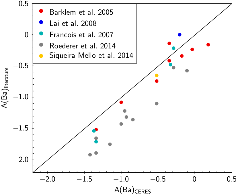
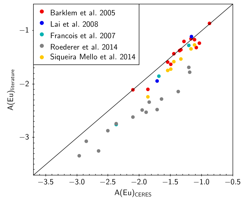
Figure 13: Comparison of our Ba and Eu abundances for the stars in common with five high resolution surveys. The black lines represent the identity function.

B.1 High resolution surveys

It is interesting to compare the yield of the CERES surveys with other surveys of comparable high resolution. The first obvious comparison is with the First Stars survey in which François et al. (2007) provided abundances of neutron capture elements for 32 giant extremely metal-poor stars. In our sample we have included five stars already analysed by François et al. (2007). Another survey to compare to is HERES (Barklem et al. 2005) that provided abundances for 253 metal-poor halo stars, almost equally split between giants and dwarfs, or subgiants. The survey was a snapshot survey, conducted with UVES at the 8.2 m VLT, but with wide slit ($2^{\prime\prime}$), low resolving power $R\sim 20\,000$ and low S/N ratio. We have in common eight stars with this survey. A third survey to compare with is that of Lai et al. (2008) who determined the abundances for a sample of 28 metal-poor stars based on high-resolution spectra obtained with HIRES at the Keck 10 m telescope. Again the sample is almost equally split between giants and dwarfs, or subgiants. We have two stars in common with this survey. Cohen et al. (2013, 0Z project) determined detailed abundances for 146 metal-poor stars from spectra obtained with HIRES at the Keck Telescope and with Mike at the 6.5 m Magellan Telescope. About half of the sample is constituted by giant stars. We have no stars in common with this sample. Roederer et al. (2014b) determined abundances for 313 stars based on spectra obtained with Mike at the Magellan telescope, with the Robert G. Tull Coudé Spectrograph on the 2.7 m Harlan J. Smith Telescope at McDonald Observatory and with the High Resolution Spectrograph on the 9.2 m Hobby–Eberly Telescope at McDonald Observatory during a ten year long observing campaign. The sample is constituted for 57% of giant and horizontal branch (HB) stars, including some blue HB stars. We have 14 stars in common with this survey. Li et al. (2022) determined abundances for 385 metal-poor stars, almost equally split among giants and dwarfs, or subgiants. The candidates were selected from the LAMOST (Deng et al. 2012; Liu et al. 2014) survey and followed up with the HDS spectrograph on the 8.2 m Subaru telescope. We have only one star in common with this survey. Of the seven elements here examined they provide only Ba, La, and Eu. Hansen et al. (2012) derived abundances of seven heavy elements (Sr, Y, Zr, Pd, Ag, Ba, and Eu) for a sample of 71 giant and dwarf stars observed at high resolution ($R>40\,000$) and high S/N ratio (¿100 per pixel at 320 nm) with UVES at VLT. We have nine stars in common with this study. Another useful comparison is with the sample of Siqueira Mello et al. (2014), who derived the abundances of the elements from Li to Th in a sample of seven stars observed at high-resolution ($R\sim 40\,000$) and high S/N ratio with UVES at VLT. All seven stars in the sample of Siqueira Mello et al. (2014) were also analysed in this study.

In Table 11 we compare the number of measures (not including upper limits) of the different surveys. It is clear that CERES is providing more detailed abundances that most of the other surveys, for most elements. The Survey with most measurements is that of Roederer et al. (2014b), that is also the one that can count on the largest investment of telescope time, and provides more measurements than we do for all elements. Ba is provided by HERES, by the 0Z project and by Li et al. (2022) for a sample that is an order of magnitude larger than ours. For Eu, however, HERES and Li et al. (2022) provide a larger sample, but in this case of the same order of magnitude as CERES, while the 0Z project provides less measurements.

In Fig. 13 we show the comparison between our abundances of Ba and Eu, respectively, and literature values for the stars in common. While the agreement with Barklem et al. (2005), Lai et al. (2008), François et al. (2007), and Siqueira Mello et al. (2014) is reasonably good, the values of Roederer et al. (2014b) are systematically lower than ours. This is also true for Fe, as pointed out in Paper I and is a result of the lower effective temperatures and gravities adopted by Roederer et al. (2014b).

One further thing to be considered is that CERES is designed to provide the measurement of as many neutron capture elements as possible, so that the real throughput of the survey in terms of achieved chemical inventory should be evaluated after all the papers in the series are published. One success of CERES, is the high S/N ratio of the observations obtained in program 0104.D-0059, and the fact that for archival spectra we benefit from high S/N ratio spectra and in some cases we could combine several spectra, as detailed in Paper I (see table A1 of that paper). The high quality of the data allows for more heavy element abundance derivations of poorly studied elements exceeding Ba and Eu (Alencastro Puls et al. 2024; Lombardo et al, in prep.) and to compare them with rare earth elements. Another reason of success in measuring abundances of neutron capture elements is that we concentrated on giant stars, similar to what done by François et al. (2007), unlike the other quoted surveys.

B.2 Individual high resolution studies

In this section we compare the results obtain in this study with the ones from individual literature studies that analysed in detail some of the stars in our sample. In Fig. 14 we show the comparison between our derived abundances of Ba, La, Ce, Pr, Nd, Sm, and Eu for the stars CES1221-0328 (HE1219-0312), CES1402+0941 (HD122563), CES2231-3238 (CS 29491-069), CES2254-4209 (HE2252-4225), and CES2330-5626 (HE2327-5642) and the ones obtained by Honda et al. (2006), Hayek et al. (2009), Mashonkina et al. (2010), and Mashonkina et al. (2014). We note that for the stars CS 29491-069, HE2327-5642, and HE2252-4225 the values are overall in good agreement, while for the stars HD122563 and HE1219-0312 we tend to have higher abundances compared to the ones in the literature. This is mostly due to the higher $\mathrm{\log g}$ derived by us for these two stars. In Table 12 the stellar parameters derived in this study are compared to the literature. We see that for the stars for which we observe the largest difference in the abundances, HD122563 and HE1219-0312, there is also a difference in the stellar parameters, particularly in $\mathrm{\log g}$ and microturbulence.

Table 11: Number of abundance measures for the different surveys

Survey	Ba	La	Ce	Pr	Nd	Sm	Eu
This paper	43	45	46	29	43	38	51
Barklem et al. 2005	220	33	13	0	35	9	68
François et al. 2007	31	17	10	14	19	7	17
Lai et al. 2008	24	3	0	0	0	0	5
Hansen et al. 2012	60	0	0	0	0	0	51
Cohen et al. 2013	111	30	21	6	27	4	27
Roederer et al. 2014	297	112	65	43	96	50	141
Siqueira Mello et al. 2014	7	7	6	4	7	6	7
Li et al. 2022	318	72	0	0	0	0	79

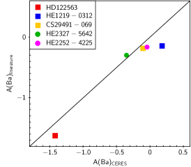
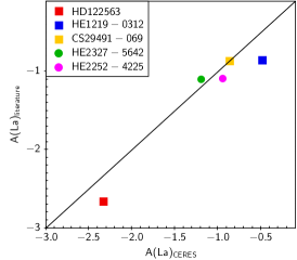
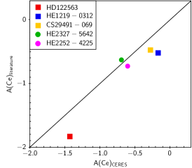
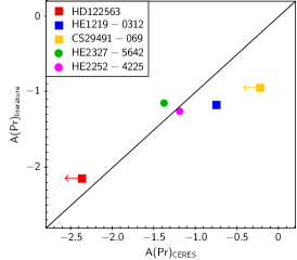
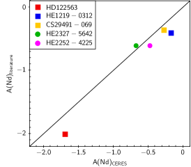
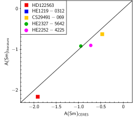
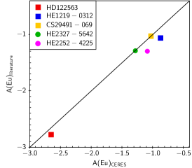
Figure 14: Comparison of our Ba, La, Ce, Pr, Nd, Sm, and Eu abundances for the stars in common with Honda et al. 2006 (HD122563), Hayek et al. 2009 (HE1219-0312, CS 29491-069), Mashonkina et al. 2010 (HE2327-5642), and Mashonkina et al. 2014 (HE2252-4225). The black lines represent the identity function.

Table 12: Comparison between stellar parameters in literature and in this paper for selected stars.

Star	Simbad name	$\mathrm{T_{eff}}$(lit.)	$\mathrm{T_{eff}}$(CERES)	logg(lit.)	logg(CERES)	vt(lit.)	vt(CERES)	[Fe/H](lit.)	[Fe/H](CERES)	ref.
CES1221-0328	HE1219-0312	5060	5145	2.30	2.76	1.60	1.60	$-$2.96	$-$2.96	1
CES1402+0941	HD122563	4570	4682	1.10	1.35	2.20	2.01	$-$2.77	$-$2.79	2
CES2231-3238	BPS CS29491-069	5300	5222	2.80	2.67	1.60	1.67	$-$2.51	$-$2.77	1
CES2254-4209	HE2252-4225	4710	4805	1.65	1.98	1.70	1.79	$-$2.63	$-$2.88	3
CES2330-5626	HE2327-5642	5050	5028	2.34	2.31	1.80	1.75	$-$2.78	$-$3.10	4

(1) Hayek et al. (2009); (2) Honda et al. (2006); (3) Mashonkina et al. (2014); (4) Mashonkina et al. (2010).

Appendix C Additional plots

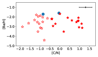
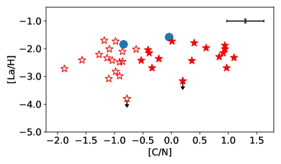
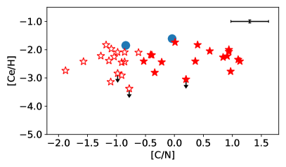
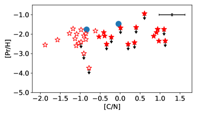
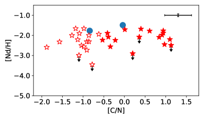
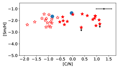
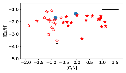
Figure 15: [Ba/H], [La/H], [Ce/H], [Pr/H], [Nd/H], [Sm/H], [Eu/H] abundances as a function of [C/N] for our sample of stars. The open/filled star symbols represent mixed/unmixed stars according to the classification in Paper II (mixed: [N/Fe]$>$0.5 and [C/N]$<$$-0.6$, unmixed: [N/Fe]$<$0.5 and [C/N]$>$$-0.6$). The filled circles represent stars that have values outside the ranges defined for mixed and unmixed stars.

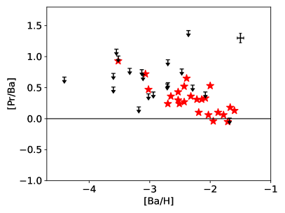
Figure 16: [Ce/Ba] and [Pr/Ba] abundance ratios as a function of [Ba/H]. The black arrows represent upper limits of abundance ratios. A representative error bar is shown in the upper-right corner of each panel.

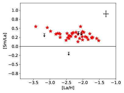
Figure 17: [Ce/La], [Pr/La], [Nd/La], [Sm/La] abundance ratios as a function of [La/H]. Coloured symbols as in Fig. 16.

Figure 18: [Pr/Ce], [Nd/Ce], [Sm/Ce] abundance ratios as a function of [Ce/H]. Coloured symbols as in Fig. 16.

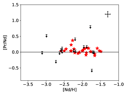
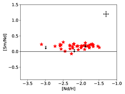
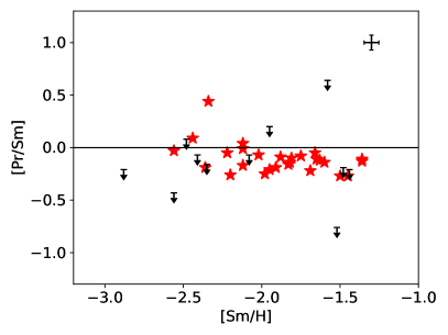
Figure 19: [Pr/Nd] and [Sm/Nd] abundance ratios as a function of [Nd/H], and [Pr/Sm] abundance ratio as a function of [Sm/H]. Coloured symbols as in Fig. 16.

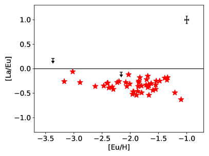
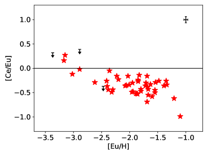
Figure 20: [La/Eu], [Ce/Eu], [Pr/Eu], [Nd/Eu] and [Sm/Eu] abundance ratios as a function of [Eu/H]. Coloured symbols as in Fig. 16.

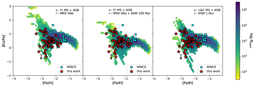
Figure 21: [Eu/Fe] abundance ratios as a function of [Fe/H] for our sample of stars (red stars) and MINCE data (François et al. 2024, cyan squares) compared to the GCE models of Cescutti & Chiappini (2014) (left), Cescutti et al. (2015) (centre), and Rizzuti et al. (2021) (right, see text for more details).