Exclusive diffractive dijets at HERA and EIC using GTMDs

Abstract

We calculate differential distributions for diffractive production of dijets in $ep\rightarrow e^{{}^{\prime}}p\,jet\,jet$ reaction using off diagonal unintegrated gluon distributions, often called GTMDs for brevity. Different models are used. We focus on the contribution to exclusive $q\bar{q}$ dijets.

The results of our calculations are compared with the H1 and ZEUS data. Except of one GTMD, our results are below the HERA data points. This is in contrast with recent results where the normalization was adjusted to some selected distributions and no agreement with other observables was checked. We conclude that the calculated cross sections are only a small part of the measured ones which probably contain also processes with pomeron remnant, reggeon exchange, etc.

We present also azimuthal correlations between the sum and the difference of dijet transverse momenta. The cuts on transverse momenta of jets generate azimuthal correlations (in this angle) which can be easily misinterpreted as due to so-called elliptic GTMD.

1 Introduction

This work focuses on exclusive, diffractive production of dijets in the $ep\to ejjp$ reaction, where the final-state proton remains in its ground state. This presentation is based on our recent publication [1]. The processes discussed there were measured by the H1 [2] and ZEUS [3] collaborations. We use a formalism derived from the color dipole approach but the dipole amplitude information from impact parameter space is mapped to off-forward transverse momentum-dependent gluon distributions (GTMDs). For reviews linking this to the gluon Wigner function, see [4]. At large jet transverse momenta, the forward diffractive amplitude directly probes the unintegrated gluon distribution of the target [5, 6]. While this approach is suited for the small-$x$ limit, longitudinal momentum transfer and skewedness are handled in a collinear factorization framework using generalized parton distributions, as in [7]. This work includes also $q\bar{q}$ exchanges in the $t$-channel, relevant for smaller rapidity gaps.

In [8], we applied various GTMD models to the $pA\to c\bar{c}pA$ process, although no data is available yet for this reaction due to several challenges of relevant measurements. Here, we apply the same formalism to $ep\to jjp$ in order to confront our results with the H1 and ZEUS data, comparing results of different GTMD models.

Recent theoretical calculations on diffractive dijet production, using either the color dipole or GTMD approaches can be found in [9, 10, 11, 12, 13, 14]. Some of these works focus on photoproduction of dijets or production of heavy quarks. Our study has some overlap with [9], which uses the Golec-Biernat–Wüsthoff parametrization [15] for the dipole amplitude. For the corresponding gluon distribution, our results agree with the other results. We employ also the GTMDs proposed and fitted in [13, 14]. However, our conclusions differ from those works.

2 Sketch of the formalism

To calculate the cross section for $ep\rightarrow ep\,q\bar{q}$ both the transverse $\sigma_{T}$ and longitudinal $\sigma_{L}$ cross sections have to be included:

$$\frac{d\sigma^{ep}}{dydQ^{2}d\xi} = \frac{\alpha_{em}}{\pi yQ^{2}}\Big{[}\Big{(}1-y+\frac{y^{2}}{2}\Big{)}\frac{d\sigma_{T}^{\gamma^{*}p}}{d\xi}+(1-y)\frac{d\sigma_{L}^{\gamma^{*}p}}{d\xi}\Big{]},$$ (1)

where $d\xi=dzd^{2}\vec{P}_{\perp}d^{2}\vec{\Delta}_{\perp}$, while the interferences between photon polarizations are neglected as they vanish when averaging over the angle between the electron scattering and the hadronic planes.

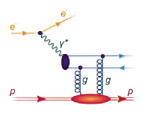
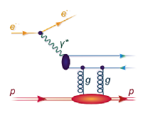
Figure 1: Four Feynman diagrams for the diffractive production of dijets in electron-proton collisions.

For all four mechanisms shown in Fig.1, the $\gamma^{*}p\to q\bar{q}p$ cross sections for transverse and longitudinal photons are given by:

$$\frac{d\sigma^{\gamma^{*}p}_{T}}{dzd^{2}\vec{P}_{\perp}d^{2}\vec{\Delta}_{\perp}} = 2N_{c}\alpha_{em}\sum_{f}e_{f}^{2}\int d^{2}\vec{k}_{\perp}\int d^{2}\vec{k}^{~{}^{\prime}}_{\perp}T\big{(}Y,\vec{k}_{\perp},\vec{\Delta}_{\perp}\big{)}T\big{(}Y,\vec{k}^{~{}^{\prime}}_{\perp},\vec{\Delta}_{\perp}\big{)}$$ (2)

$$\times \Bigg{\{}\Big{(}z^{2}+(1-z)^{2}\Big{)}\left[\frac{(\vec{P}_{\perp}-\vec{k}_{\perp})}{(\vec{P}_{\perp}-\vec{k}_{\perp})^{2}+\epsilon^{2}}-\frac{\vec{P}_{\perp}}{P^{2}_{\perp}+\epsilon^{2}}\right]$$

$$\cdot \left[\frac{(\vec{P}_{\perp}-\vec{k}^{~{}^{\prime}}_{\perp})}{(\vec{P}_{\perp}-\vec{k}^{~{}^{\prime}}_{\perp})^{2}+\epsilon^{2}}-\frac{\vec{P}_{\perp}}{P^{2}_{\perp}+\epsilon^{2}}\right]$$

$$+ m_{f}^{2}\left[\frac{1}{(\vec{P}_{\perp}-\vec{k}_{\perp})^{2}+\epsilon^{2}}-\frac{1}{P^{2}_{\perp}+\epsilon^{2}}\right]$$

$$\cdot \left[\frac{1}{(\vec{P}_{\perp}-\vec{k}^{~{}^{\prime}}_{\perp})^{2}+\epsilon^{2}}-\frac{1}{P^{2}_{\perp}+\epsilon^{2}}\right]\Bigg{\}},$$

$$\frac{d\sigma^{\gamma^{*}p}_{L}}{dzd^{2}\vec{P}_{\perp}d^{2}\vec{\Delta}_{\perp}} = 2N_{c}\alpha_{em}4Q^{2}z^{2}(1-z)^{2}$$ (3)

$$\times \sum_{f}e_{f}^{2}\int d^{2}\vec{k}_{\perp}\int d^{2}\vec{k}^{~{}^{\prime}}_{\perp}T\big{(}Y,\vec{k}_{\perp},\vec{\Delta}_{\perp}\big{)}T\big{(}Y,\vec{k}^{~{}^{\prime}}_{\perp},\vec{\Delta}_{\perp}\big{)}$$

$$\times \left[\frac{1}{(\vec{P}_{\perp}-\vec{k}_{\perp})^{2}+\epsilon^{2}}-\frac{1}{P^{2}_{\perp}+\epsilon^{2}}\right]$$

$$\cdot \left[\frac{1}{(\vec{P}_{\perp}-\vec{k}^{~{}^{\prime}}_{\perp})^{2}+\epsilon^{2}}-\frac{1}{P^{2}_{\perp}+\epsilon^{2}}\right],$$

with $\epsilon^{2}=z(1-z)Q^{2}+m_{f}^{2}$ and the generalized transverse momentum distribution (GTMD) of gluons in the proton target are expressed as a Fourier transform of the diffraction amplitude in momentum space (see [10, 11, 12, 4]):

$$T(Y,\vec{k}_{\perp},\vec{\Delta}_{\perp})=\int\frac{d^{2}\vec{b}_{\perp}}{(2\pi)^{2}}\frac{d^{2}\vec{r}_{\perp}}{(2\pi)^{2}}e^{-i\vec{\Delta}_{\perp}\cdot\vec{b}_{\perp}}e^{-i\vec{k}_{\perp}\cdot\vec{r}_{\perp}}\,N(Y,\vec{r}_{\perp},\vec{b}_{\perp})\,e^{-\varepsilon r_{\perp}^{2}}\,.$$ (4)

The used normalization is consistent with that in Ref. [12] and the regularization parameter $\varepsilon=(0.5\,\rm{fm})^{-2}$ is used in the calculation. We also analyzed special correlations in azimuthal angle between the sum and difference of transverse momenta of jets:

$$\cos\phi_{\vec{P}_{\perp}\vec{\Delta}_{\perp}}=\frac{\vec{P}_{\perp}\cdot\vec{\Delta}_{\perp}}{P_{\perp}\Delta_{\perp}}\,,$$ (5)

where

$$\vec{P}_{\perp}=\frac{1}{2}(\vec{p}_{\perp 1}-\vec{p}_{\perp 2})\,,\qquad\vec{\Delta}_{\perp}=\vec{p}_{\perp 1}+\vec{p}_{\perp 2}\,.$$ (6)

In [1] we considered six different models for generalized transverse momentum distributions (GTMDs). Two of these are parameterizations of off-forward gluon density matrices based on diagonal unintegrated gluon distributions: Golec-Biernat–Wüsthoff (GBW) model [15] and Moriggi-Paccini-Machado (MPM) model [16]. Both use a diffractive slope of $B=4$ $\rm GeV^{-2}$:

$$f\Big{(}Y,\frac{\vec{\Delta}_{\perp}}{2}+\vec{k}_{\perp},\frac{\vec{\Delta}_{\perp}}{2}-\vec{k}_{\perp}\Big{)}=\frac{\alpha_{s}}{4\pi N_{c}}\,\frac{{\cal F}(x_{\mathrm{I\!P}},\vec{k}_{\perp},-\vec{k}_{\perp})}{k_{\perp}^{4}}\,\exp\Big{[}-\frac{1}{2}B\vec{\Delta}^{2}\Big{]}\,.$$ (7)

The other four distributions are derived from the Fourier transform of the dipole amplitude described by equation (4).

We use also the bSat model of Kowalski and Teaney [17] (KT model), as well as three models based on the McLerran-Venugopalan (MV) approach [18]. These include the Iancu-Rezaeian model (MV-IR) [19], the Boer-Setyadi 2021 model (MV-BS 2021) [13], and the Boer-Setyadi 2023 model (MV-BS 2023) [14], which were fitted to the H1 experimental data. In addition, we modified the MV-IR model using $\lambda=0.277$:

$$T_{\rm MV-IR}^{\rm mod}(Y,\vec{k}_{\perp},\vec{\Delta}_{\perp})=T_{\rm MV-IR}(\vec{k}_{\perp},\vec{\Delta}_{\perp})\,e^{\lambda Y},\quad\,Y=\ln\Big{[}\frac{0.01}{x_{\mathrm{I\!P}}}\Big{]}\,.$$ (8)

To adopt the MV-BS 2021 to describe the H1 data [2] we added according to  [13] $\chi=1.25$ in the expression:

$$N_{0}(r_{\perp},b_{\perp})=-\frac{1}{4}r_{\perp}^{2}\chi Q_{s}^{2}(b_{\perp})\ln\Big{[}\frac{1}{r_{\perp}^{2}\lambda^{2}}+e\Big{]},\,Q_{s}^{2}(b_{\perp})=\frac{4\pi\alpha_{s}C_{F}}{N_{c}}\exp\Big{[}\frac{-b_{\perp}^{2}}{2R_{p}^{2}}\Big{]}.$$ (9)

For MV-BS 2023 the $\chi(x_{Bj})=\bar{\chi}\Big{(}\frac{x_{0}}{x_{Bj}}\Big{)}^{\lambda_{\chi}},$ where $\bar{\chi}=1.5,\,x_{0}=0.0001$ and $\lambda_{\chi}=0.29$ are used according to  [14].

3 Selected results

Our calculations were divided into two areas according to the kinematics of the H1 and ZEUS collaborations. We first show the distributions in the transverse momentum of the jet shown in Fig. 2. The MV-BS 2021 and MV-BS 2023 give similar results to the MV-IR and MPM models and describe the data quite well, while the KT and GBW distributions are lower by an order of magnitude than the experimental data. Both the MV-BS results for the ZEUS kinematics differ by almost two orders of magnitude from the results of other GTMDs, however, the shapes of all distributions are similar. We also generated distributions in $x_{\mathrm{I\!P}}$ and $\beta$ shown in Fig. 3, where the differences between all models are visible. In the case of the dependence on $x_{\mathrm{I\!P}}$, the data are overestimated by all GTMD models except of those based on KT and GBW UGDFs, see Eq.(7). This may be related to the fact that correct description of all experimental data requires considering not only the dipole approach but also the contribution of $q\bar{q}$ exchanges, see e.g. Ref. [20].

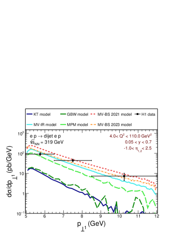
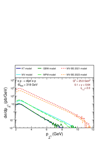
Figure 2: Distribution of the cross-section for the diffractive light-quark dijet production in jet transverse momentum for H1 (left) and ZEUS (right) kinematics for different GTMDs.

The distributions in $\beta$ also show inconsistencies with the experimental data for the MV-BS models that were fitted to the H1 experiment. In contrast, the other models give results that are below experimental data for small $\beta$, However, this area can be sensitive to the $q\bar{q}g$ three-parton contributions.

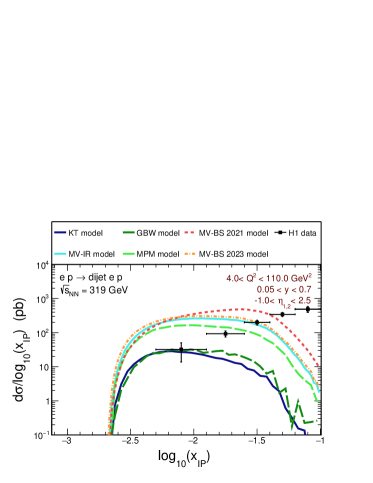
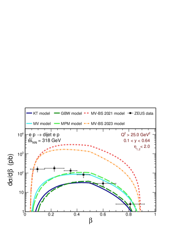
Figure 3: Distribution of the cross-section for the diffractive light-quark dijet production in $x_{\mathrm{I\!P}}$ and $\beta$ for H1 and ZEUS kinematic for different GTMDs.

In Fig. 4 we show the distribution of the azimuthal angle between the sum and difference of the jets’ transverse momenta. We predict that the straight horizontal line corresponds to the case without cuts on the transverse momentum of the jets, while the angular correlations can be seen for the situation in which such cuts are included. We do not exclude the possibility that the additional azimuthal correlation may be due to elliptical gluon distributions, which were not taken into account in [1].

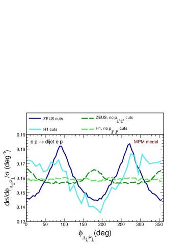
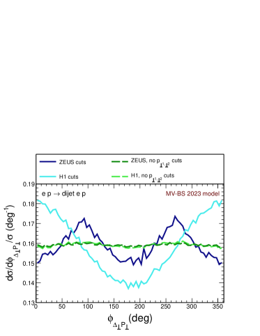
Figure 4: Distribution of the cross-section for the diffractive light-quark dijet production in the energy of the photon-proton system (left) and azimuthal angle $\phi$ between $\vec{P}_{\perp}$ and $\vec{\Delta}_{\perp}$ (right) for H1 and ZEUS kinematic for different GTMDs. The reader is asked to notice the normalization.

4 Conclusions

We have discussed dijet production in the $ep\rightarrow epjj$ process. The corresponding differential distributions have been calculated using various gluon GTMD (generalized transverse momentum dependent gluon distributions) from the literature. We have calculated the distributions in various kinematic variables by referring to H1 and ZEUS data. The MV-BS, MPM, and MV-IR GTMD distributions describe some of the observables quite well but do not describe the distributions in $x_{\mathrm{I\!P}}$ and $\beta$. Some of the other GTMD distributions are consistent with the H1 and ZEUS data. In our opinion the most realistic gluon distributions are those based on KT and GBW, which give rather small contribution for the H1 kinematics, and a sizable contribution at $\beta>0.5$ for the ZEUS cuts. We conclude that the considered gluonic mechanism is not sufficient. Therefore we plan to continue the topic.

We have also calculated correlations in azimuthal angles between the sum and difference of the jet’s transverse momenta. Since our GTMDs do not have an elliptical part, these correlations are solely the result of experimental cuts.

Acknowledgements

A.S. is indebted to Marta Łuszczak and Wolfgang Schäfer for collaboration on the issues presented here.

References

[1]
B. Linek, M. Łuszczak, W. Schäfer and A. Szczurek,
Phys. Rev. D 110 054027 (2024).
[2]
F. Aaron et al., Eur. Phys. J. C 72, 1970 (2012).
[3]
H. Abramowicz et al., Eur. Phys. J. C 76, 16 (2016).
[4]
R. Pasechnik and M. Taševský, (2023), arXiv:2310.10793 [hep-ph].
[5]
N. N. Nikolaev and B. G. Zakharov, Phys. Lett. B 332, 177
(1994).
[6]
N. N. Nikolaev, W. Schäfer, and G. Schwiete, Phys. Rev. D 63, 014020 (2001).
[7]
V. M. Braun and D. Y. Ivanov, Phys. Rev. D 72, 034016 (2005), arXiv:hep-ph/0505263.
[8]
B. Linek, A. Luszczak, M. Luszczak, R. Pasechnik, W. Schäfer,
and A. Szczurek, JHEP 10, 179 (2023).
[9]
R. Boussarie, A. V. Grabovsky, L. Szymanowski, and S. Wallon, Phys. Rev. D 100, 074020 (2019).
[10]
Y. Hagiwara, Y. Hatta, and T. Ueda, Phys. Rev. D 94, 094036 (2016).
[11]
Y. Hagiwara, Y. Hatta, R. Pasechnik, M. Tasevsky, and O. Teryaev, Phys. Rev. D 96, 034009 (2017).
[12]
M. Reinke Pelicer, E. Gräve De Oliveira, and R. Pasechnik, Phys. Rev. D 99, 034016 (2019).
[13]
D. Boer and C. Setyadi, Phys. Rev. D 104, 074006 (2021).
[14]
D. Boer and C. Setyadi, Eur. Phys. J. C 83, 890 (2023).
[15]
K. J. Golec-Biernat and M. Wüsthoff, Phys. Rev. D 59, 014017 (1998).
[16]
L. S. Moriggi, G. M. Peccini, and M. V. T. Machado, Phys. Rev. D 102, 034016 (2020).
[17]
H. Kowalski and D. Teaney, Phys. Rev. D 68, 114005 (2003).
[18]
L. D. McLerran and R. Venugopalan, Phys. Rev. D 49, 3352 (1994).
[19]
E. Iancu and A. H. Rezaeian, Phys. Rev. D 95, 094003 (2017).
[20]
M. Łuszczak, R. Maciuła, and A. Szczurek,
Phys. Rev. D 91, 054024 (2015).