MMD-OPT : Maximum Mean Discrepancy Based Sample Efficient Collision Risk Minimization for Autonomous Driving

Abstract

We propose MMD-OPT: a sample-efficient approach for minimizing the risk of collision under arbitrary prediction distribution of the dynamic obstacles. MMD-OPT is based on embedding distribution in Reproducing Kernel Hilbert Space (RKHS) and the associated Maximum Mean Discrepancy (MMD). We show how these two concepts can be used to define a sample efficient surrogate for collision risk estimate. We perform extensive simulations to validate the effectiveness of MMD-OPT on both synthetic and real-world datasets. Importantly, we show that trajectory optimization with our MMD-based collision risk surrogate leads to safer trajectories at low sample regimes than popular alternatives based on Conditional Value at Risk (CVaR).

Note to Practitioners

Autonomous Driving software stacks have dedicated modules for predicting trajectories of the obstacles(neighboring vehicles). Typically, these predictors provide a set of possible future motions for the obstacles, each of which can have different likelihoods of happening. Thus, a key challenge is to reason about collision risk in a given scene based on predicted trajectories, but without being overly conservative. For example, treating each predicted trajectory as a separate obstacle, without any attention to their likelihood, may not allow any feasible motion to the ego-vehicle. Our work addresses this challenge by proposing a probabilistic approach for modeling and minimizing collision risk. Our core impact lies in improving sample efficiency: that is assessing and minimizing collision risk based on just a handful of predicted trajectories for a given obstacle. Our approach can be easily integrated with any deep neural network based trajectory predictors which have become the de facto standard in autonomous driving industry. Our formulation easily extends to applications like indoor navigation with mobile robots, since human trajectory predictors have structural similarity with those deployed in autonomous driving. A practical limitation of our approach is that it requires additional computing power (in the form of GPU accelerators) to achieve real-time performance.

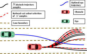
Figure 1: The figure shows a scenario where an obstacle has multiple intents (lane-change vs lane-following), each associated with a trajectory distribution. However, both intents have wildly different probabilities. In this particular example, the probability of lane-change is higher. For safe navigation, the ego-vehicle needs to consider this multi-modal nature of obstacle trajectories while planning its own motions. Our proposed approach estimates the more likely samples (the reduced-set) from a set of obstacle trajectories sampled from a black-box distribution. This allows us to plan probabilistically safe motions while appropriately discriminating the low and high-probability obstacle manoeuvres.

I Introduction

Ensuring collision avoidance between the ego vehicle and the dynamic (neighbouring vehicles) obstacles is a fundamental requirement in autonomous driving. This in turn, requires predicting the trajectories of the latter over a time horizon. It is often difficult to predict just one deterministic trajectory for the dynamic obstacles because of the uncertainty associated with its intentions and the deployed sensors. Thus, existing works [1], [2], [3] are focused on predicting a distribution of trajectories that can capture their various likely motions.

The objective of this paper is to leverage the predictions from off-the-shelf trajectory predictors in the best possible manner for safe motion planning. Specifically, the core emphasis is on developing a risk cost that captures the probability of collision given trajectory predictions of the dynamic obstacles. This collision risk cost can then be minimized with any off-the-shelf optimizer along with other costs associated with control, smoothness and lane adherence.

There are two core challenges with regards to developing a collision risk cost. First, the analytical form of prediction distribution may be intractable or unknown. For example, the state-of-the-art trajectory predictors like [1],[4],[5],[6] characterize the predicted trajectory distribution in the form of deep generative models that can be arbitrary complex with multiple modes. Thus, existing collision risk derived from chance-constraints under Gaussian uncertainty [7],[8],[9],[10] become unsuitable.

Second, due to the complex nature of the predicted distribution, we often just have access to samples drawn from it. In such a case, the collision risk cost should be amenable to sample efficient estimation. That is, it should capture the true probability of collision with just a few samples of predicted obstacle trajectories. The sample efficiency is also directly related to computational run-time. The use of higher number of predicted trajectory samples translates to an increase in the number of collision checks between the ego and the obstacles.

In this paper, we propose MMD-OPT: a trajectory optimizer combined with a sample efficient surrogate for collision risk. The foundation of our work is built around estimating how different two given distributions are. For example, in the case of Gaussian, this can be calculated using the Kullback-Liebler (KL) divergence. However, computing the dissimilarity between arbitrary distributions is often intractable. One possible workaround is to compute the difference between two distributions in the Reproducing Kernel Hilbert Space (RKHS) [11], [12]. Specifically, given only drawn samples, we can represent the underlying distribution as a point in RKHS. Moreover, the difference between the two embedding can be easily captured by the so-called Maximum Mean Discrepancy (MMD) measure.

Algorithmic Contribution: MMD-OPT uses the concept of RKHS embedding and MMD in two novel ways which also forms our core algorithmic contribution. First, given a set of predicted obstacle trajectories, we embed the underlying distribution of collision constraint residuals in RKHS. Subsequently we define a collision risk surrogate as the MMD between the RKHS embedding of collision constraint residuals and Dirac-Delta distribution. The advantage of our MMD-based surrogate is that we can systematically improve its sample efficiency by leveraging the underlying properties of RKHS embedding and MMD. To this end, we propose a bi-level optimization problem that tells us which of the obstacle trajectory samples can be disregarded without compromising the ability of our MMD-based surrogate to capture the true probability of collision(see Fig.1). This in turn, reduces the number of collision checks required to reliably produce safe trajectories and adds to the overall sample and computational efficiency of MMD-OPT. Finally, we propose a custom sampling-based optimizer to minimize MMD-based collision risk surrogate along with driving discomfort in the form of sharp accelerations and lane boundary violations.

State-of-the-Art Performance: We empirically compare planning with our MMD-based collision risk surrogate with that achieved using popular risk-cost alternatives derived from Sample Average Approximation (SAA) [13] and Conditional Value at Risk (CVaR) [14]. We show that our approach leads to safer trajectories for a given number of samples of obstacle trajectories. The difference is more prominent when the underlying prediction distribution departs significantly from the Gaussian form. We also demonstrate that our approach is computationally fast enough for real-time applications.

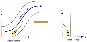
Figure 2: The image shows that nonlinear reference paths (such as curvy roads) are represented by straight lines on the $s$-axis in Frenet coordinates. However, motions that do not exactly follow the reference path result in nonlinear motions in Frenet coordinates. Instead, such motions result in an offset from the reference path and therefore the $s$-axis, which is described with the $d$ coordinate.

II Problem Formulation and Preliminaries

Symbols and Notations

Scalars will be represented by normal-font small-case letters, while bold-faced variants will represent vectors. We will use upper-case bold fonts to represent matrices. Symbol $k$ will represent the discrete-time step while $T$ will represent the transpose operator.

II-A Motion Model in Frenet Frame

We formulate trajectory planning of the ego-vehicle in the road-aligned reference frame known as the Frenet frame(Fig 2). In this setting, the curved roads can be treated as ones with straight-line geometry. This is achieved by aligning the longitudinal and lateral motions of the ego-vehicle with the axes of the Frenet frame. Specifically, in Frenet coordinates, we use two variables, namely, $s$ representing longitudinal displacement or the distance along the reference path and $d$ representing the lateral displacement or perpendicular offset from the reference path. The $s$ coordinate starts with $s=0$ at the beginning of the reference path. Lateral coordinates on the reference path are represented with $d=0$. Depending on the convention used for the Frenet frame, $d$ is positive to the left or right of the reference path.

We adopt the following bi-cycle model in the Frenet frame for the ego-vehicle [15], where in the subscript $k$ represents the time-step.

$$s_{k+1} =s_{k}+\dot{s}_{k}\Delta t,d_{k+1}=d_{k}+\dot{d}_{k}\Delta t$$ (1a)

$$\psi_{k+1} =\psi_{k}+\dot{\psi}_{k}\Delta t,v_{k+1}=v_{k}+a_{k}\Delta t$$ (1b)

$$\dot{s}_{k+1} =\frac{v_{k}\cos\psi_{k}}{1-d_{k}\kappa(s_{k})},\dot{d}_{k+1}=v_{k}\sin\psi_{k}$$ (1c)

$$\dot{\psi}_{k+1} =\frac{v_{k}\tan(\theta_{k})}{B}-\kappa(s_{k})\frac{v_{k}\cos\psi_{k}}{1-d_{k}\kappa(s_{k})},$$ (1d)

where $\psi_{k}$ is the heading of the ego-vehicle in the Frenet Frame and $B$ is the wheelbase of the car. The ego-vehicle is driven by a combination of longitudinal acceleration $a_{k}$ and steering input $\theta_{k}$. The variable $\kappa(s_{k})$ is the curvature of the reference path at the longitudinal coordinate $s_{k}$.

Differential Flatness The motion model (1a)-(1d) is differentially flat. That is, we can represent the control inputs as a function of position and its derivatives. More precisely, we have

$$v_{k} =\sqrt{(\dot{s}_{k}(1-d_{k}\kappa(s_{k})))^{2}+(\dot{d}_{k})^{2}},a_{k}=\frac{v_{k+1}-v_{k}}{\Delta t}$$ (2)

$${\psi}_{k} =\tan^{-1}(\dot{d}_{k},\dot{s}_{k}),\dot{\psi}_{k}=\frac{\psi_{k+1}-\psi_{k}}{\Delta t}$$ (3)

$$\theta_{k} =\tan^{-1}\left(\frac{(\dot{\psi}_{k}+\kappa(s_{k})\dot{s}_{k})B}{v_{k}}\right)$$ (4)

II-B Risk-Aware Trajectory Optimization

Let $\boldsymbol{\tau}_{k}$ represent the obstacle position at time-step $k$. Let $\boldsymbol{\tau}\in\mathbb{R}^{2H}$ denote the obstacle trajectory formed by stacking time-stamped way-points over a planning horizon $H$. In the stochastic case, $\boldsymbol{\tau}$ is a random variable with distribution $p_{\boldsymbol{\tau}}$. With these notations in place, we can leverage differential flatness to formulate risk-aware trajectory optimization directly in the trajectory space as shown below:

$$\min_{\mathbf{s},\mathbf{d}}c(\mathbf{s}^{(q)},\mathbf{d}^{(q)})+r(\mathbf{s},\mathbf{d},\boldsymbol{\tau})$$ (5)

$$\mathbf{h}(\mathbf{s}^{(q)},\mathbf{d}^{(q)})=\mathbf{0}$$ (6)

$$\textbf{g}(\mathbf{s}^{(q)},\mathbf{d}^{(q)})\leq 0,\forall k$$ (7)

$${\mathbf{s}}{{}^{(q)}}=(s^{(q)}_{1},s^{(q)}_{2},\dots,s^{(q)}_{k},\dots,s^{(q)}_{H})$$

$${\mathbf{d}}{{}^{(q)}}=(d^{(q)}_{1},d^{(q)}_{2},\dots,d^{(q)}_{k},\dots,d^{(q)}_{H}),q={0,1,2}$$

The first term in the cost (5) minimizes some function $c(\cdot)$ defined over the $q^{th}$ derivative of the position variable. We can use the differential flatness property to roll any state and control dependent cost into this term. The second term, $r(\cdot)$ models the collision risk of the ego-vehicle colliding with the predicted trajectory $\boldsymbol{\tau}$ of the obstacle. The equality constraints enforce the initial and final boundary conditions on the planned ego trajectory. The inequality constraints (7) model the different kinematic and geometric constraints (e.g. lane boundary) that need to be satisfied by the optimal trajectory. We provide the exact mathematical form for these constraints in Section VI.

Remark 1.

For ease of exposition, the problem formulation (5)-(7) only considers the case of a single neighbouring vehicle that acts as an obstacle to the ego-vehicle. Thus, we only have one random obstacle trajectory $\boldsymbol{\tau}$. The extension to arbitrary traffic density is trivial.

Remark 2.

The Optimization (5)-(7) is solved under the assumption that we can draw samples of $\boldsymbol{\tau}$ from $p_{\boldsymbol{\tau}}$ but the parametric form for the latter is not known. Moreover, sampling is relatively cheap compared to the computational cost of estimating the risk $r$(defined below) from the predicted samples of obstacle trajectories.

II-C Exact Collision Risk

Let $f_{k}({s}_{k},d_{k},\boldsymbol{\tau}_{k})$ represent the collision constraint function at time step $k$, such that $f_{k}\leq 0,\forall k$ ensures collision avoidance. Then, we can define the worst-case collision-constraint value ($f$) in the following manner.

$$f(\mathbf{s},\mathbf{d},\boldsymbol{\tau})=\max_{k}(f_{k}({s}_{k},d_{k},\boldsymbol{\tau}_{k}))$$ (8)

where we recall that $\boldsymbol{\tau}_{k}=(s_{o,k},d_{o,k})$ is the position of the obstacle at time-step $k$ and is obtained from the trajectory predictor. Stacking $\boldsymbol{\tau}_{k}$ at different time steps gives us $\boldsymbol{\tau}$. There are several ways to define $f_{k}({s}_{k},d_{k},\boldsymbol{\tau}_{k})$. In the most general setting, this can be a black box function derived from 3D occupancy maps [16]. We can also derive an analytical form for $f_{k}({s}_{k},d_{k},\boldsymbol{\tau}_{k})$ if we approximate the shape of ego and the neighbouring in terms of geometric primitives such as ellipses.

In the stochastic setting, when $\boldsymbol{\tau}$ is a random variable, $f$ provides a distribution of the worst-case collision-constraint value. Thus, using (8), we can define collision risk through (9), wherein $P$ denotes the probability.

$$r=P(f(\mathbf{s},\mathbf{d},\boldsymbol{\tau})\geq 0).$$ (9)

The r.h.s of (9) maps the ego and the obstacle trajectory to the probability that the worst-case collision-constraint value is greater than zero and thus, indicating an imminent collision. Thus, minimizing $r$ within (5)-(7) will produce safer trajectories. However, the main computational challenge stems from the fact that for arbitrary obstacle trajectory distribution, $p_{\boldsymbol{\tau}}$, the r.h.s of (9) does not even have an analytical expression. This necessitates the development of approximations/surrogates that can achieve a similar effect as $r$ while being computationally more tractable. This is discussed next.

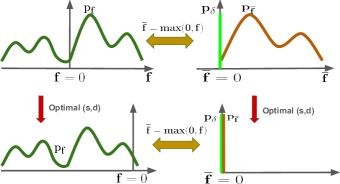
Figure 3: Figure shows the distribution ($p_{f}$) of worst-case collision constraint value ($f$). The distribution ($p_{\overline{f}}$) shows the distribution of collision-constraint residuals. Note that by definition, the mass of $p_{\overline{f}}$ lies to the right of $\overline{f}=0$. We want the mass of $p_{f}$ to lie completely to the left of $f=0$. Thus, the risk-aware trajectory optimization is essentially finding the ego-vehicle trajectory that reshapes the distribution of $p_{f}$ in appropriate form. Moreover, as the mass of $p_{f}$ shifts to the left, the distribution $p_{\overline{f}}$ converges to a Dirac-Delta distribution.

II-D Sample Approximation of Risk Metric

In this sub-section, we will use the samples of obstacle trajectories to approximate $r$. We begin by defining the collision constraint residual function $\overline{f}$ in the following manner

$$\overline{f}=\max(0,f(\mathbf{s},\mathbf{d},\boldsymbol{\tau}))$$ (10)

The $\overline{f}$ as defined in (10) maps the distribution over ego and obstacle trajectories to a distribution over collision constraint residuals. The relationship between the probability distribution of $f$ and $\overline{f}$ is shown in Fig.3. Now, assume that we have access to $N$ samples of obstacle trajectories ${{}^{j}}\boldsymbol{\tau},\forall j=1,2,\dots N$ drawn from $p_{\boldsymbol{\tau}}$. The different approximations of $r$ revolve around using the obstacle trajectories to obtain samples of $\overline{f}$ and computing appropriate empirical statistics on them.

II-D1 Sample Average Approximation (SAA) Risk Estimate

A simple yet effective approximation of collision risk $r$ (9) can be obtained by simply averaging the collision constraint residuals across different samples of the predicted trajectories [13], [17]. That is we have

$$r_{SAA} =\frac{1}{N}\sum_{j=1}^{N}\mathbb{I}\left({{}^{j}}\overline{f}(\mathbf{s},\mathbf{d},{{}^{j}}\boldsymbol{\tau})>0\right)$$ (11)

where $\mathbb{I}(\cdot)$ is an indicator function returning 1 when the conditions in the operand are satisfied and 0 otherwise. In essence, (11) minimizes the frequency of constraint violation over the samples of predicted obstacle trajectories. Although conceptually simple, estimates of the form (11) have proved useful in the existing literature [13].

II-D2 Conditional Value at Risk (CVaR) based Risk Estimate

An alternative sample approximation of collision risk can be obtained by computing the empirical/sample estimate of CVaR of $\overline{f}$, using the samples $\{^{j}\overline{f}\}_{j=1}^{j=N}$ [18],[14],[19]. That is we define the risk metric as

$$r_{CVaR}^{emp}=CVaR_{\alpha}^{emp}(\overline{f})$$ (12)

where $\alpha$ is some tuneable parameter associated with CVaR. We can follow the approach in [14] to compute $CVaR_{\alpha}^{emp}(\overline{f})$

III Preliminaries on Kernels and Reproducing Kernel Hilbert Space(RKHS)

This section introduces the concept of a kernel, feature map and Reproducing Kernel Hilbert space (RKHS) which forms the backbone of our approach MMD-OPT. For a detailed exposition of these topics, refer [20].

III-A Feature Maps and Kernels

Let $\mathcal{X}$ be a measurable input space. Consider a vector $\mathbf{z}\in\mathcal{X}$ and a non-linear transformation $\phi$ called feature-map. We can use $\phi$ to embed $\mathbf{z}$ in the RKHS $\mathcal{H}$([20] Section 2.2) as $\phi(\mathbf{z})$. A positive definite real-valued kernel function $K:\mathcal{X}\times\mathcal{X}\rightarrow\mathbb{R}$ is related to the feature map through the so-called kernel trick $K(\mathbf{z},\mathbf{z}^{\prime})=\langle\phi(\mathbf{z}),\phi(\mathbf{z}^{\prime})\rangle_{\mathcal{H}}$ ([20] Definition 2.1), where $\langle\cdot,\cdot\rangle_{\mathcal{H}}$ is an inner product in $\mathcal{H}$. Intuitively, the inner product provides the distance between $\mathbf{z},\mathbf{z}^{{}^{\prime}}$ in RKHS. The kernel trick has the following implication: to compute the inner product $\langle\phi(\mathbf{z}),\phi(\mathbf{z}^{\prime})\rangle_{\mathcal{H}}$, we do not have to explicitly compute $\phi(\mathbf{z})$. Instead, we just need to evaluate the kernel function over the pair $\mathbf{z},\mathbf{z}$ as $K(\mathbf{z},\mathbf{z}^{\prime})$ and this will give us the required inner product. We use the Laplace Kernel throughout our implementation. It is given by:

$$K(\mathbf{z},\mathbf{z}^{\prime})=\exp{\left(-\frac{\parallel\mathbf{z}-\mathbf{z}^{\prime}\parallel_{1}}{\sigma}\right)}$$ (13)

where $\parallel\cdot\parallel_{1}$ denotes the $l^{1}$ norm(also known as the Manhattan or Taxicab norm). Here $\sigma>0$ is a tuneable bandwidth parameter.

III-B From data points to probability distributions

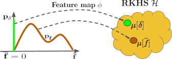
Figure 4: Kernel mean embedding of probability distributions $p_{\delta}$ and $p_{\overline{f}}$ into RKHS $\mathcal{H}$

We can generalize the concept of a feature map, kernel function and RKHS embedding to work on probability distributions as well (see Figure 4). Let $u$ be a random variable with probability distribution $p_{u}$. The RKHS embedding of $u$ ( or $p_{u}$) is given by the following.

$$\mu[u]=\int K(u,.)dp(u)$$ (14)

Essentially, (14) maps probability distribution to a function in RKHS. For arbitrary distribution $p_{u}$, it is often intractable to compute the r.h.s of (14). Thus, instead, we can resort to the empirical estimate of the RKHS embedding. Let ${{}^{j}}u$ be samples of $u$ drawn from $p_{u}$. The empirical estimate of $\mu[u]$ is given by the following.

$$\widehat{\mu}[u]:=\sum_{j=1}^{N}\frac{1}{N}\phi(^{j}{u})=\sum_{j=1}^{N}\frac{1}{N}K(^{j}{u},\cdot)$$ (15)

Functions of Random Variables

We can extend the concept of RKHS embedding to functions of random variables as well. Let $g(u)\in\mathcal{X}\rightarrow\mathcal{Z}$ be an arbitrary function of a random variable $u$ with $p_{g}$ denoting the probability distribution of $g(u)$. Its RKHS embedding $\mu[g]$ and its empirical estimate $\hat{\mu}[g]$ is given by

$$\mu[g]=\int K(g(u),.)dp(u),\quad\widehat{\mu}[g]=\sum_{j=1}^{N}\frac{1}{N}K(g(^{j}{u}),\cdot),$$ (16)

Note that $K$ in the above expressions (16) is the same as that used in (15).

One of the attractive features of RKHS embedding is that when constructed with characteristic Kernels (Gaussian, Laplacian, etc.), it can capture information about mean and moments of $u$ and $g(u)$ up to infinite order. Furthemore, $\widehat{\mu}[u],\widehat{\mu}[g]$ are consistent estimators. That is they converge to the true RKHS embedding as we increase the sample size $N$. The RKHS embeddings $\widehat{\mu}[u],\widehat{\mu}[g]$ are also tightly coupled through the following theorem from [11].

Theorem 1.

Suppose $g$ is a continuous function and the kernel functions are continuous and bounded. Then, the following holds

$$\text{if}\hskip 5.69046pt\hat{\mu}[u]\rightarrow\mu[u],\hskip 5.69046pt\text{then}\hskip 5.69046pt\hat{\mu}[g]\rightarrow\mu[g]$$ (17)

The proof can be found in the Appendix of [11].

III-C Maximum Mean Discrepancy and Improving Sample Efficiency

One of the core applications of RKHS embedding lies in quantifying similarity/difference between two probability distributions through a concept called Maximum Mean Discrepancy (MMD) defined in the following manner.

Definition 1.

Let $u$ and $\tilde{u}$ be two random variables with probability distributions $p_{u}$ and $p_{\tilde{u}}$ respectively. The MMD between the two distributions is given by

$$MMD(p_{u},p_{\tilde{u}})=\left\|\mu[u]-{\mu}[\tilde{u}\right\|_{\mathcal{H}}^{2}=\left\langle\mu[u]-{\mu}[\tilde{u}],\mu[u]-{\mu}[\tilde{u}]\right\rangle$$ (18)

where $\left\|(.)\right\|_{\mathcal{H}}$ is the RKHS norm and can be expressed through inner products, which in turn can be evaluated using the Kernel trick. The distribution $p_{u}$ and $p_{\tilde{u}}$ are same if and only if $\left\|\mu[u]-{\mu}[\tilde{u}\right\|_{\mathcal{H}}^{2}=0$ [11], [21]. Typically, it is intractable to obtain the exact MMD and thus, we resort to its empirical estimate given by the following

$$MMD^{emp}(p_{u},p_{\tilde{u}})=\left\|\hat{\mu}[u]-\hat{\mu}[\tilde{u}\right\|_{\mathcal{H}}^{2}$$ (19)

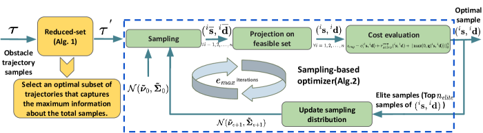
Figure 5: Overview of MMD-OPT. It consists of two main parts. The first part is the so-called reduced-set algorithm that tells us which obstacle trajectories can be discarded without compromising the ability of our MMD-based surrogate to capture the collision risk in a given scene. The second part is a sampling-based optimizer the minimizes the MMD-based collision risk cost. Our sampling based optimizer also consists of novel components that exploits the problem structure for computational efficiency.

IV Main Algorithmic Results

This section presents our main algorithmic contributions. An overview of our approach is shown in Fig. 5. The cornerstone of our work is the reduced-set selection (Alg.1) which allows us to use only a subset of predicted obstacle trajectories to compute our MMD-based collision risk surrogate. This in turn, drastically reduces the number of collision-checks that we need to perform. The optimal reduced-set is then passed to the downstream sampling-based optimizer(Alg.2) wherein we sample trajectories in the Frenet-frame from a Gaussian distribution and evaluate their associated costs (including collision risk). The sampling distribution is updated in an iterative fashion to drive the costs down at each iteration.

In the next few sub-sections, we present the different components from Fig.5. We begin by presenting our surrogate for collision risk.

IV-A Collision Risk as Difference of Two Distributions

The distribution of ${f}$ and $\overline{f}$, denoted by $p_{f}$ and $p_{\overline{f}}$ respectively, cannot be characterized analytically, even if we assume that the predicted trajectory of the neighbouring vehicle is drawn from a Gaussian distribution. In general, $p_{\boldsymbol{\tau}}$ can be arbitrarily complex, making it even more challenging to make any assumption on the nature of $p_{f}$ and $p_{\overline{f}}$. However, we can intuitively reason about some desired characteristics that the latter two distribution should have.

• As shown in Fig.3, we want to shift the mass of distribution $p_{f}$ to the left of $f=0$. The higher the mass is to the left of $f=0$, the lower the risk $r=P(f\geq 0)$.

• As the mass of $p_{f}$ gets shifted to the left of $f=0$, $p_{\overline{f}}$ converges to a Dirac-Delta distribution $p_{\delta}$. This follows directly from the definition of $\overline{f}$ in (10).

• We can re-imagine risk-aware trajectory optimization as the problem of finding the optimal ego vehicle trajectory $(\mathbf{s},\mathbf{d})$ that re-shapes $p_{\overline{f}}$ to look similar to a Dirac-Delta distribution. This, in turn, would ensure that the mass of $p_{f}$ gets shifted to the left of $f=0$.

Based on the above insights, we propose the following novel surrogate for collision risk

$$r_{MMD}=MMD(p_{\overline{f}},p_{\delta})=\left\|\mu[\overline{f}]-\mu[\delta]\right\|_{\mathcal{H}}^{2},$$ (20)

where $\mu[\overline{f}]$ is the RKHS embedding of $\overline{f}$ (or $p_{\overline{f}}$) defined in the following manner

$$\mu[\overline{f}]=\int K(\overline{f},.)dp_{\overline{f}}(\overline{f}),\quad\widehat{\mu}[\overline{f}]=\sum_{j=1}^{N}\frac{1}{N}\phi({{}^{j}}\overline{f}),$$ (21)

It is connected to the RKHS embedding of obstacle trajectory distribution $p_{\boldsymbol{\tau}}$ defined as:

$$\mu[\boldsymbol{\tau}]=\int K(\boldsymbol{\tau},.)dp_{\boldsymbol{\tau}}(\boldsymbol{\tau}),\quad\widehat{\mu}[\boldsymbol{\tau}]=\sum_{j=1}^{N}\frac{1}{N}\phi(^{j}\boldsymbol{\tau}),$$ (22)

Similarly, $\mu[\delta]$ is the RKHS embedding of a random variable $\delta\sim p_{\delta}$. As $r_{MMD}$ decreases, $p_{\overline{f}}$ becomes similar to $p_{\delta}$. In the limiting case, as $r_{MMD}\rightarrow 0$, the distribution $p_{\overline{f}}\rightarrow p_{\delta}$ and consequently $P(f\geq 0)\rightarrow 0$.

Since the true $r_{MMD}$ is intractable to compute for arbitrary $p_{\boldsymbol{\tau}}$, we will be working with the following empirical estimate computed through sample-level information

$$r_{MMD}^{emp}=\left\|\hat{\mu}[\overline{f}]-\hat{\mu}[\delta]\right\|_{\mathcal{H}}^{2}$$ (23)

Remark 3.

By Theorem 1, $\hat{\mu}[\boldsymbol{\tau}]\rightarrow{\mu}[\boldsymbol{\tau}]$ implies $\hat{\mu}[\overline{f}]\rightarrow{\mu}[\overline{f}]$ and consequently $r_{MMD}^{emp}\rightarrow r_{MMD}$

Remark 4.

We can approximate $p_{\delta}$ through a Gaussian $\mathcal{N}(0,\epsilon)$, with an extremely small covariance $\epsilon$ ($\approx 10^{-5}$).

Finite Sample Guarantees

A key advantage of $r_{MMD}^{emp}$ is that it inherits the excellent convergence and finite sample gurantees associated with RKHS embedding and MMD. Specifically, how far $r_{MMD}^{emp}$ is from the true $r_{MMD}$ can be quantified by the following Theorem that is a direct application of the result presented in [12].

Theorem 2.

Let $\overline{f},\delta$ be the collision constraint violation and Dirac-Delta random variables respectively. Let $p_{\overline{f}},p_{\delta}$ be the respective probability distributions of $\overline{f}$ and $\delta$. Given samples $X:=\{^{j}\overline{f}\}_{j=1}^{j=N}$ and $Y:=\{\delta_{j}\}_{j=1}^{j=N}$ i.i.d from $p_{\overline{f}}$ and $p_{\delta}$ , respectively, and assuming $0\leq K(\xi_{1},\xi_{2})\leq c_{o},\forall\xi_{1},\xi_{2}$ and some constant $c_{o}$, then:

$$P_{X,Y}\biggl{\{}|r_{MMD}^{emp}-r_{MMD}|\leq 2\Bigl{(}2(c_{o}/N)^{\frac{1}{2}}+\varepsilon\Bigr{)}\biggr{\}}$$

$$>1-\exp\Bigl{(}\frac{-\varepsilon^{2}N}{4c_{o}}\Bigr{)}$$ (24)

where $P_{X,Y}$ denotes the probability over the $N$-sample $X$ and $Y$, and $\varepsilon>0$ is an arbitrary parameter controlling the probability bound. $K(x,y)$ denotes the kernel function.

Theorem 2 ensures that as the sample size $N$ increases, the probability that the absolute difference between $r_{MMD}^{emp}$ and $r_{MMD}$ tends to a small value approaches $1$. In other words, with increase in samples, not only the estimate $r_{MMD}^{emp}$ improves, the stochasticity or the variance associated with it also reduces. In Section VI, we show Theorem 2 directly translates to lower worst-case collision-rate with $r_{MMD}^{emp}$ as compared to $r_{CVaR}^{emp}$ and $r_{SAA}$.

IV-B Advantages of $r_{MMD}^{emp}$ as a Collision Risk Surrogate

Just like $r_{SAA}$ (Eqn. (11)) and $r_{CVaR}$ (Eqn. (12)), our $r_{MMD}^{emp}$ also requires evaluating the collision constraint residual function $\overline{f}$ over predicted obstacle trajectories. This can be computationally intensive if the collision checks are expensive. The key feature that differentiates $r_{MMD}^{emp}$ from $r_{SAA}$ and $r_{CVaR}^{emp}$ is that we can use the tools from RKHS embedding and MMD to systematically improve its sample complexity. In other words, we can use only a subset $N^{{}^{\prime}}<<N$ of the predicted obstacle trajectories to evaluate $\overline{f}$ and yet incur only minimum degradation in estimation of $r_{MMD}^{emp}$. We call this subset as reduced-set following the notation from [11], [12].

Let ${}^{l}\boldsymbol{\tau}^{{}^{\prime}},l=1,2,3,\dots N^{{}^{\prime}}$ be the reduced-set formed by sub-selecting $N^{{}^{\prime}}$ samples out of $N$ samples of $\boldsymbol{\tau}$. Moreover, let us attach weights ${{}^{l}}\beta$ with every ${}^{l}\boldsymbol{\tau}^{{}^{\prime}}$ such that $\sum_{l}{{}^{l}}\beta=1$. Let ${{}^{l}}\overline{f^{^{\prime}}}$ be the samples of $\overline{f}$ evaluated on ${}^{l}\boldsymbol{\tau}^{{}^{\prime}}$. The empirical RKHS emebeddings of $p_{\boldsymbol{\tau}}$ and $p_{\overline{f}}$ computed using ${}^{l}\boldsymbol{\tau}^{{}^{\prime}}$ and ${{}^{l}}\overline{f^{^{\prime}}}$ are given by

$$\hat{\mu}[\boldsymbol{\tau}^{{}^{\prime}}]=\sum_{l}{{}^{l}}\beta\phi({{}^{l}}\boldsymbol{\tau}^{{}^{\prime}}),\qquad\hat{\mu}[\overline{f^{^{\prime}}}]=\sum_{l}{{}^{l}}\beta\phi({{}^{l}}\overline{f^{^{\prime}}})$$ (25)

Now, [11] showed that Theorem 1 can also be leveraged to ensure that if $\hat{\mu}[\boldsymbol{\tau}^{{}^{\prime}}]$ is close to $\hat{\mu}[\boldsymbol{\tau}]$ in MMD metric, then $\hat{\mu}[\overline{f^{\prime}}]$ will be close to $\hat{\mu}[\overline{f}]$ in the same metric. Consequently, $r_{MMD}^{emp}$ computed using $\hat{\mu}[\overline{f^{\prime}}]$ which requires $N^{{}^{\prime}}$ predicted obstacle trajectories will be closer to that computed using $\hat{\mu}[\overline{f}]$ on the larger set of $N$ samples. Alternately, if we reduce the sample size in a way that we minimize $\left\|\hat{\mu}[\boldsymbol{\tau}^{{}^{\prime}}]-\hat{\mu}[\boldsymbol{\tau}]\right\|_{\mathcal{H}}^{2}$, the loss of accuracy in estimation of $r_{MMD}^{emp}$ will be minimal. In the next sub-section, we present several ways by which this can be achieved.

IV-C Reduced-Set

There are three ways to minimize $\left\|\hat{\mu}[\boldsymbol{\tau}^{{}^{\prime}}]-\hat{\mu}[\boldsymbol{\tau}]\right\|_{\mathcal{H}}^{2}$. First, we can choose the reduced-set in a careful manner. Second, we optimize the values of ${{}^{l}}\beta$. Finally, we can also the choose the right set of kernel parameter $\sigma$. In the subsequent subsections, we first present a simple method that adopts only the second approach and is a straightforward application of [11]. Subsequently, we present our key result that adopts all the three ways to minimize $\left\|\hat{\mu}[\boldsymbol{\tau}^{{}^{\prime}}]-\hat{\mu}[\boldsymbol{\tau}]\right\|_{\mathcal{H}}^{2}$.

IV-C1 Fixed Reduced-Set, Optimal Weights

In this approach, we assume that the $N^{^{\prime}}$ reduced-set samples ${{}^{l}}\boldsymbol{\tau}^{{}^{\prime}}$ are simply a random sub-selection from $N$ samples of $\boldsymbol{\tau}$. We then optimize the weights of the ${{}^{l}}\boldsymbol{\tau}^{{}^{\prime}}$ through the following optimization problem.

$$\min_{{{}^{l}}\beta}\left\|\frac{1}{N}\sum_{i=1}^{i=N}\phi(^{i}{\boldsymbol{\tau}})-\sum_{l=1}^{l={N}^{^{\prime}}}{{}^{l}}\beta\phi({{}^{l}\boldsymbol{\tau}^{^{\prime}}})\right\|_{\mathcal{H}}^{2}$$ (26a)

$$\sum_{l}{{}^{l}}\beta=1$$ (26b)

Using the kernel-trick, optimization (26a)-(26b) can be rephrased as an equality-constrained QP. Essentially, (26a)-(26b) can be seen as distilling the information from a significantly larger sample set of predicted obstacle trajectories to the reduced-set by re-weighting the importance of the samples of the latter.

IV-C2 Optimal Reduced-Sets, Weights and Kernel Parameters

In this approach, we simultaneously optimize the selection of the reduced-set, the weights of its individual samples and kernel parameters. Our approach takes the form of a bi-level optimization (27a)-(LABEL:bi_level_inner_red_cost), wherein $\mathbf{O}$ is a matrix with $N$ rows, each containing a sample of $\boldsymbol{\tau}$ drawn from $p_{\boldsymbol{\tau}}$.

$$\min_{\boldsymbol{\lambda},\sigma} \left\|\frac{1}{{N}}\sum_{i=1}^{i={N}}\phi(^{i}{\boldsymbol{\tau}})-\sum_{l=1}^{l={N}^{^{\prime}}}{{}^{l}}\beta^{*}\phi(^{l}\boldsymbol{\tau}^{^{\prime}})\right\|_{\mathcal{H}}^{2}$$ (27a)

$$F_{\boldsymbol{\lambda}}({\mathbf{O}})=(^{1}\boldsymbol{\tau}^{^{\prime}},^{2}\boldsymbol{\tau}^{^{\prime}},\dots,^{N^{\prime}}\boldsymbol{\tau}^{^{\prime}})$$ (27b)

$${{}^{l}}\beta^{*}=\begin{aligned} &&&\arg\min_{{{}^{l}}\beta}\left\|\frac{1}{{N}}\sum_{i=1}^{i={N}}\phi(^{i}{\boldsymbol{\tau}})-\sum_{l=1}^{l={N}^{^{\prime}}}{{}^{l}}\beta\phi(^{l}\boldsymbol{\tau}^{^{\prime}})\right\|_{\mathcal{H}}^{2}\\ &&&\operatorname{s.t.}\sum{{{}^{l}}\beta}=1\end{aligned}$$ (27c)

In (27a)-(LABEL:bi_level_inner_red_cost), $F_{\boldsymbol{\lambda}}$ is a selection function that chooses $N^{^{\prime}}$ rows out of $\mathbf{O}$ to form the reduced-set. It is parameterized by $\boldsymbol{\lambda}$. That is, different $\boldsymbol{\lambda}$ leads to different reduced-set. We discuss the algebraic form for $F_{\boldsymbol{\lambda}}$ later in this section. But, it is worth pointing out that if we fix $\boldsymbol{\lambda}$ and consequently $F_{\boldsymbol{\lambda}}$ (e.g just a random $\boldsymbol{\lambda}$ ) and the kernel parameter $\sigma$, then we recover the earlier approach described in (26a)-(26b).

As can be seen, the inner optimization (LABEL:bi_level_inner_red_cost) is defined over just the weights ${{}^{l}}\beta$ for a fixed $\boldsymbol{\lambda}$. The outer optimization in turn optimizes in the space of $\boldsymbol{\lambda}$ and kernel parameter in order to reduce the MMD cost associated with optimal ${{}^{l}}\beta^{*}$. Our bi-level approach provides two pronged benefits. First, it gets rid of the variance associated with randomly selecting the reduced-set. Second, our approach leads to $\hat{\mu}[\boldsymbol{\tau}^{^{\prime}}]$ that has lower MMD difference from $\hat{\mu}[\boldsymbol{\tau}]$ as compared to that achieved from the previous method of Section IV-C1. This in turn, improves the embedding of $\hat{\mu}[\overline{f^{^{\prime}}}]$ and consequently the estimate of $r_{MMD}^{emp}$.

Selection Function $F_{\boldsymbol{\lambda}}$: Let $\boldsymbol{\lambda}\in\mathbb{R}^{{N}}$ be an arbitrary vector and $\lambda_{t}$ be its $t^{th}$ element. Assume that $|\lambda_{t}|$ encodes the value of choosing the $t^{th}$ row of $\mathbf{O}$ to form the reduced-set. That is, larger the $|\lambda_{t}|$, the higher the impact of choosing the $t^{th}$ row of ${\mathbf{O}}$ in minimizing (27a). With these constructions in place, we can now define $F_{\boldsymbol{\lambda}}$ through the following sequence of mathematical operations.

$$\mathcal{S}=Argsort\{|\lambda_{1}|,|\lambda_{2}|,\dots|\lambda_{N}|)\}$$ (28a)

$$\mathbf{O}^{{}^{\prime}}=[{\mathbf{O}}_{t_{1}},{\mathbf{O}}_{t_{2}},\dots,{\mathbf{O}}_{t_{N}}],\forall t_{e}\in\mathcal{S}$$ (28b)

$$F_{\boldsymbol{\lambda}}({\mathbf{O}})=\mathbf{O}^{{}^{\prime}}_{t_{N-N^{^{\prime}}}:t_{N}}=({{}^{1}}\boldsymbol{\tau}^{^{\prime}},{{}^{2}}\boldsymbol{\tau}^{^{\prime}},\dots,{{}^{N^{^{\prime}}}}\boldsymbol{\tau}^{^{\prime}})$$ (28c)

As can be seen, we first sort in increasing value of $|\lambda_{t}|$ and compute the required indices $t_{e}$. We then use the same indices to shuffle the rows of $\mathbf{O}$ in (28b) to form an intermediate variable $\mathbf{O}^{{}^{\prime}}$. Finally, we choose the last $N^{^{\prime}}$ rows of $\mathbf{O}^{{}^{\prime}}$ as our reduced-set in (28c). Intuitively, (28a)-(28c) parameterizes the sub-selection of the rows of ${\mathbf{O}}$ to form the reduced-set. That is, different $\boldsymbol{\lambda}$ gives us different reduced-sets. Thus, a large part of solving (27a)-(LABEL:bi_level_inner_red_cost) boils down to arriving at the right $\boldsymbol{\lambda}$. We achieve this through a combination of gradient-free search and quadratic programming (QP). We present the details of our approach next.

Solution Process: Our approach for solving (27a)-(LABEL:bi_level_inner_red_cost) is presented in Alg.1 that combines gradient-free Cross-Entropy Method (CEM) [22] and QP. The input to the algorithm is the set ${\mathbf{O}}$ and the required size of the reduced-set $N^{^{\prime}}$. The output is the reduced-set samples, their weights and the optimal kernel parameter $\sigma$. Alg.1 begins by initializing a Gaussian distribution (Line 2) with mean $\boldsymbol{\nu}_{e}$ and covariance $\boldsymbol{\Sigma}_{e}$ at iteration $e=0$. The loop defined between lines 3-15 is the outer CEM optimizer. At each iteration of CEM, we sample $n_{cem}$ batch of $\boldsymbol{\lambda}$ and $\sigma$. Note that the dimension of $\boldsymbol{\lambda}$ is equal to the number of obstacle trajectory samples contained in ${\mathbf{O}}$. Subsequently, between Lines 7-12, we loop through each sampled ${{}^{m}}\boldsymbol{\lambda}$ and ${{}^{m}}\sigma$ and use them to formulate and solve the inner optimization problem. First, we use $F_{\boldsymbol{\lambda}}(\mathbf{O})$ as defined in (28a)-(28c) to obtain the reduced-set samples. These are then used to solve optimization (LABEL:bi_level_inner_red_cost) along with ${}^{m}\sigma$ as the kernel parameter to obtain ${{}^{l}}\beta^{*}$. At line 10, we compute the optimal MMD resulting from our choice of ${{}^{l}}\boldsymbol{\tau}^{^{\prime}}$ samples, ${{}^{l}}\beta^{*}$ and ${}^{m}\sigma$ and append it to our cost-list. Lines 13-14 refines the sampling distribution of the outer loop. We select the top $n_{elite}$ samples of ${{}^{m}}\boldsymbol{\lambda}$ and ${{}^{m}}\sigma$ that led to the lowest MMD cost and call it the $EliteSet$. Line 14 estimates the empirical mean and covariance over the ${{}^{m}}\boldsymbol{\lambda}$ and ${{}^{m}}\sigma$ contained in the $EliteSet$.

Alg.1 uses GPU parallelization to achieve computational efficiency. Specifically, the inner QP loop in lines 7-12 can be performed in parallel over different $m$. Moreover, we also leverage the fact that the equality constrained QP (LABEL:bi_level_inner_red_cost) have a closed-form solution. Fig.6 validates the efficacy of Alg.1 in solving (27a)-(LABEL:bi_level_inner_red_cost): the outer-level cost gradually decreases with iterations.

Validating the Efficacy of the optimal reduced-set: To empirically showcase the importance of our optimal reduced-set, we sampled $500$ obstacle trajectories to form ${\mathbf{O}}$. We then sub-selected $N^{^{\prime}}$ rows from it, either randomly or by solving the bi-level optimization (27a)-(LABEL:bi_level_inner_red_cost). We perform a large number of random sub-selections to compute the average, minimum and maximum of $\left\|\hat{\mu}[\boldsymbol{\tau}^{{}^{\prime}}]-\hat{\mu}[\boldsymbol{\tau}]\right\|_{\mathcal{H}}^{2}$. Moreover, we compute the same MMD over the optimal reduced-set as well. As can be seen from Fig.6(b), $\left\|\hat{\mu}[\boldsymbol{\tau}^{{}^{\prime}}]-\hat{\mu}[\boldsymbol{\tau}]\right\|_{\mathcal{H}}^{2}$ over the optimal reduced-set performs close to the best-case performance that we can obtain by exhaustively trying out different random reduced-sets. The performance difference is more stark at lower $N^{\prime}$. It should be noted that in real-world setting, exhaustive search is prohibitive and thus, (27a)-(LABEL:bi_level_inner_red_cost) provides a computationally efficient one-shot solution. Fig.6(c) shows that the advantages of optimal reduced-set translates to empirical embedding $\hat{\mu}[\overline{f^{^{\prime}}}]$ as well, with $\left\|\hat{\mu}[\overline{f}]-\hat{\mu}[\overline{f^{^{\prime}}}]\right\|_{\mathcal{H}}^{2}$ being only slightly inferior to the best-case value obtained with exhaustive sampling of reduced-set.

Fig.6 validates our hypothesis that minimizing $\left\|\hat{\mu}[\boldsymbol{\tau}^{{}^{\prime}}]-\hat{\mu}[\boldsymbol{\tau}]\right\|_{\mathcal{H}}^{2}$ and $\left\|\hat{\mu}[\overline{f}]-\hat{\mu}[\overline{f^{^{\prime}}}]\right\|_{\mathcal{H}}^{2}$ ensures minimal loss in the estimation of $r_{MMD}^{emp}$. To this end, we computed

$$\Delta_{r_{MMD}}=\left|\left\|\sum_{j=1}^{N}\frac{1}{N}\phi(^{j}\overline{f})-\sum_{j=1}^{j=N}\frac{1}{N}\phi(^{j}\delta)\right\|_{\mathcal{H}}^{2}-\left\|\sum_{l=1}^{N^{^{\prime}}}{{}^{l}}\beta\phi(^{l}\overline{f^{^{\prime}}})-\sum_{l=1}^{l=N^{^{\prime}}}\frac{1}{N^{^{\prime}}}\phi(^{l}\delta)\right\|_{\mathcal{H}}^{2}\right|.$$ (29)

The first term is the $r_{MMD}^{emp}$ computed on the larger set of $N$ samples, while the second term is the same computed on the smaller reduced-set. Like before, we constructed the reduced-set either randomly or by solving (27a)-(LABEL:bi_level_inner_red_cost). As shown in Fig.6, the $\Delta_{r_{MMD}}$ obtained with the optimal reduced-set is close to the average error that can be achieved by exhaustively trying different choices of the reduced-set.

1 $e_{cem}$ = Maximum number of iterations, ${N}$= size of ${\mathbf{O}}$, $N^{^{\prime}}$ = size of reduced-set

2 Initialize mean and covariance $\boldsymbol{\nu}_{e},\boldsymbol{\Sigma}_{e}$, respectively, at $e=0$ for sampling and sorting $\boldsymbol{\lambda}$ and the kernel $\sigma$ parameter respectively .

3 for $e=1,e\leq e_{cem},e++$ do

4    Draw ${n}_{cem}$ samples $({{}^{1}}\boldsymbol{\lambda},{{}^{2}}\boldsymbol{\lambda},{{}^{m}}\boldsymbol{\lambda},\dots{}^{n_{cem}}\boldsymbol{\lambda})$ and $({{}^{1}}\sigma,{{}^{2}}\sigma,{{}^{m}}\sigma,\dots{}^{n_{cem}}\sigma)$ from $\mathcal{N}(\boldsymbol{\nu}_{e},\boldsymbol{\Sigma}_{e})$.

5    ${{}^{m}}\boldsymbol{\lambda}=({{}^{m,1}}\lambda,{{}^{m,2}}\lambda,\dots{}^{m,{N}}\lambda)$ // The dimension of ${{}^{m}}\boldsymbol{\lambda}$ is equal to the rows of ${\mathbf{O}}$

6    Initialize $CostList$ = []

7   

8   for $m=1,m\leq{n}_{cem},m++$ do

9       $({{}^{1}}\boldsymbol{\tau}^{^{\prime}},{{}^{2}}\boldsymbol{\tau}^{^{\prime}},{{}^{l}}\boldsymbol{\tau}^{^{\prime}},\dots,{{}^{N^{^{\prime}}}}\boldsymbol{\tau}^{^{\prime}})=F_{{{}^{m}}\boldsymbol{\lambda}}({\mathbf{O}})$ // Reduced-Set selection formulated as sorting of the elements of ${{}^{m}}\boldsymbol{\lambda}$

10       ${{}^{l}}\beta^{*}\leftarrow$ Solve optimization (LABEL:bi_level_inner_red_cost) with the reduced-set formed above and with kernel parameter ${{}^{m}}\sigma$

11       $cost_{mmd}\leftarrow$ Compute MMD cost in (LABEL:bi_level_inner_red_cost) using ${{}^{l}}\beta^{*}$

12       append $cost_{mmd}$ to $CostList$

13      

14    end for

15   $EliteSet\leftarrow$ Select top $n_{elite}$ samples of $({{}^{m}}\boldsymbol{\lambda})_{m=1}^{m=n_{cem}}$ and $({{}^{m}}\sigma)_{m=1}^{m=n_{cem}}$ with lowest cost from $CostList$.

16    $\boldsymbol{\nu}_{e+1},\boldsymbol{\Sigma}_{e+1}\leftarrow$ Update distribution based on $EliteSet$ // Empirical mean and covariance estimate from the ElliteSet samples

17 end for

return $({{}^{1}}\boldsymbol{\tau}^{^{\prime}},{{}^{2}}\boldsymbol{\tau}^{^{\prime}},\dots,{{}^{N^{^{\prime}}}}\boldsymbol{\tau}^{^{\prime}})$, weights ${{}^{l}}\beta^{*}$ and optimal kernel hyperparameter $\sigma$ corresponding to lowest cost in the $EliteSet$

Algorithm 1 Reduced-Set Selection and Weight and Kernel Parameter Optimization using Cross-Entropy Method (CEM)

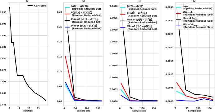
Figure 6: Validation of performance of Alg.1. Fig.(a) shows the progression of outer-level cost (27a) across iterations. Fig.(b) validates the efficacy of our optimal reduced-set selection. We sampled different random reduced-sets and computed the average, minimum and maximum of MMD $\|\hat{\mu}[\boldsymbol{\tau}^{{}^{\prime}}]-\hat{\mu}[\boldsymbol{\tau}]\|_{\mathcal{H}}^{2}$. As shown in Fig.(b), our optimal reduced-set leads to an $\|\hat{\mu}[\boldsymbol{\tau}^{{}^{\prime}}]-\hat{\mu}[\boldsymbol{\tau}]\|_{\mathcal{H}}^{2}$ that is very close to what can be achieved by exhaustively trying out different randomly selected reduced-set. Fig.(b) validates our hypothesis based on Theorem 1 and insights from [11]. As $\hat{\mu}[\boldsymbol{\tau}^{^{\prime}}]\rightarrow\hat{\mu}[\boldsymbol{\tau}]$, the MMD $\|\hat{\mu}[\overline{f}]-\hat{\mu}[\overline{f^{^{\prime}}}]\|_{\mathcal{H}}^{2}\rightarrow 0$. We can once again observe that our optimal reduced-set performs close to the best-case performance than can be hoped to be achieved by trying-out different random reduced-sets. Fig.(c) verifies that our optimal reduced-set selection ensures minimal loss in estimation of $r_{MMD}^{emp}$ while reducing the sample size. To this end, we computed $\Delta_{r_{MMD}}$ through (29) which captures the estimation error between $r_{MMD}^{emp}$ computed over a large set and the smaller reduced-set. As can be seen, $r_{MMD}^{emp}$ computed over the optimal reduced-set samples perform close to the average performance that can be achieved by exhaustively trying out different random choices of the reduced-set. It should be noted that in real-world setting, exhaustive sampling is not possible and our bi-level optimization (27a)-(LABEL:bi_level_inner_red_cost) provides a one-shot solution that is as good as exhaustive sampling in expectation.

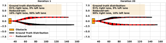
Figure 7: The figures demonstrate the physical significance of the trajectory samples used to form the optimal reduced-set. We generate a synthetic multi-modal trajectory distribution that capture the different lane-change intent of a dynamic obstacle (orange rectangle). More importantly, due to our specific generation procedure, we know the approximate probability of each lane-change intent. When Alg.1 starts, due to our random initialization of $\boldsymbol{\lambda}$, the optimal reduced-set is formed with primarily less likely trajectory samples. For example in the left figure, the reduced-set samples are mostly formed by the left lane-change maneuvers which is less likely. But as Alg.1 makes progress, the composition significantly changes. For example, in the right figure, the majority of the reduced-set samples flip from left-lane to the right-lane maneuvers. Thus, by just minimizing MMD between two sets of trajectory samples, Alg.1 is able to implicitly infer which trajectory samples are more likely and accordingly split the composition of the optimal reduced-set between the less and more likely samples.

Physical Manifestation of Optimal Reduced-Set: We now present additional empirical analysis which sheds more light into the concept of optimal reduced-set. Specifically, we analyze if the obstacle trajectory samples contained in the optimal reduced-set have a physical significance. To this end, consider Fig.7 which shows a synthetic multi-modal obstacle trajectory distribution that spans two different lane-change intents. This distribution were generated by sampling set-points for lateral offsets (from the lane center-line) and forward velocity from a binomial distribution and a Gaussian Mixture Model respectively and mapping those to trajectory distribution using the planner presented in Appendix VIII-A. Due to discrete nature of the lateral offset set-point distribution, we can approximately infer which of the lane-change maneuvers of Fig.7 are more likely. We now apply Alg.1 to choose a subset of trajectory samples to form the optimal reduced-set. We visualize the chosen samples in Fig.7. As can be seen, at the first iteration of Alg.1, the optimal reduced-set is primarily formed by less likely samples from the distribution. But as Alg.1 makes progress and the outer MMD cost (27a) comes down, the composition of the optimal reduced-set drastically changes. Specifically, more samples of more likely trajectories are found in the optimal reduced-set at later iterations. In fact, the split of more and less likely trajectory samples in the optimal reduced-set closely follow the ground-truth probability. We observed this trend consistently across all our simulations, and we believe, it points to an interesting emergent behavior in Alg.1. To summarize, although, Alg.1 does not use the actual probability of a trajectory sample in any way, it finds an implicit way of inferring the more likely samples by just minimizing the MMD between two sets of trajectory samples. This in turn, ensures that $r_{MMD}^{emp}$ constructed on the optimal reduced-set demonstrates excellent ability to capture collision risk and thus lead to safer motions.

IV-D Trajectory Optimizer

We minimize (5) subject to (6)-(7) with $r_{MMD}^{emp}$ as our risk cost, through sampling-based optimization that combines features from CEM [22], Model Predictive Path Integral (MPPI)[23] and its modern variants [24]. These class of optimizer operate by drawing at each iteration, a batch of ego-vehicle trajectories from a parametric distribution and evaluating the cost over all of them. Subsequently, the cost values are used to adapt the parameters of the sampling distribution for the next iteration. Typically, these optimizer are used in unconstrained setting. Thus, to account for inequality constraints (7), we embed a projection optimizer into the sampling pipeline that is responsible for pushing the sampled trajectories towards feasible region (e.g lane boundary) before evaluating their cost.

Our proposed sampling-based optimizer is presented in Alg.2. The input to our algorithm is the allowable iteration limit and the optimal reduced-set samples computed from Alg.1. We leverage the problem structure by sampling trajectories in Frenet-Frame. To this end, we first sample ${n}$ behavioural inputs ${{}^{i}}\textbf{b}$ such as desired lateral offsets and longitudinal velocity set-points from a Gaussian distribution (line 4). These are then fed into a Frenet space planner inspired by [25] in line 6, effectively mapping the distribution over behavioural inputs to that over trajectories. We present the details about the Frenet planner in Appendix VIII. The obtained trajectories are then passed in line 7 to a projection optimization that pushes the trajectories towards a feasible region. Our projection optimizer is built on top of [26], [27] and can be easily parallelized over GPUs. In line 8, we evaluate the constraint residuals over the projection outputs $({{}^{i}}\mathbf{s},{{}^{i}}\mathbf{d})$. In line 9, we select top $n_{c}(<n)$ projection outputs with the least constraint residuals. We call this set the $ConstraintEliteSet$. In line 10, we form $c_{aug}$ that consists of the primary cost (5) augmented with the constraint residual. In line 11-12, we append $c_{aug}$ to the $CostList$. In line 13, we extract the top $n_{elite}(\leq n_{c})$ trajectory samples form $ConstraintEliteSet$ that led to the lowest $c_{aug}$. We call this the $EliteSet$. In line 14, we update the sampling distribution of behavioural inputs based on the cost samples collected in the $EliteSet$. The exact formula for mean and covariance update is presented in (30a)-(30b). Herein, the constants $\gamma$ and $\eta$ are the temperature and learning rate respectively.

The notion of $EliteSet$ is brought from classic CEM, while the mean and covariance update follow from MPPI [23], and [24]. An important feature of Alg.2 is we have effectively encoded long horizon trajectories with a low dimensional behavioural input vector samples ${{}^{i}}\mathbf{b}$. This, in turn, improves the computational efficiency of our approach.

$$\boldsymbol{\tilde{\nu}}_{e+1}=(1-\eta)\boldsymbol{\tilde{\nu}}_{e}+\eta\frac{\sum_{i=1}^{i=n_{elite}}{{}^{i}\omega}\hskip 2.84544pt{{}^{i}}\mathbf{b}}{\sum_{i=1}^{i=n_{elite}}{{}^{i}\omega}},$$ (30a)

$$\boldsymbol{\tilde{\Sigma}}_{e+1}=(1-\eta)\boldsymbol{\tilde{\Sigma}}_{e}+\eta\frac{\sum_{i=1}^{i=n_{elite}}{{}^{i}\omega}({{}^{i}}\mathbf{b}-\boldsymbol{\tilde{\nu}}_{e+1})({{}^{i}}\mathbf{b}-\boldsymbol{\tilde{\nu}}_{e+1})^{T}}{\sum_{i=1}^{i=n_{elite}}{{}^{i}\omega}}$$ (30b)

$${{}^{i}\omega}=\exp{\frac{-1}{\gamma}(c_{aug}({{}^{i}}\mathbf{s},{{}^{i}}\mathbf{d})})$$ (30c)

1 $e_{max}$ = Maximum number of iterations, reduced-set samples of obstacle trajectories $({{}^{1}}\boldsymbol{\tau}^{^{\prime}},{{}^{2}}\boldsymbol{\tau}^{^{\prime}},\dots{}^{N^{^{\prime}}}\boldsymbol{\tau}^{^{\prime}})$ and kernel parameter $\sigma$ from Alg.1

2 Initiate mean $\boldsymbol{\tilde{\nu}}_{e},\boldsymbol{\tilde{\Sigma}}_{e}$, at $e=0$ for sampling Frenet-Frame behavioural inputs $\mathbf{b}$

3 for $e=1,e\leq e_{max},e++$ do

4    Draw ${n}$ samples $({{}^{1}}\mathbf{b},{{}^{2}}\mathbf{b},\dots{}^{i}\mathbf{b},\dots,{{}^{n}}\mathbf{b})$ from $\mathcal{N}(\boldsymbol{\tilde{\nu}}_{e},\boldsymbol{\tilde{\Sigma}}_{e})$

5    Initialize $CostList$ = []

6   

7   Query Frenet-planner for $\forall^{i}\mathbf{b}$: $({{}^{i}}\mathbf{\overline{s}},{{}^{i}}\mathbf{\overline{d}})=\text{Frenet Planner}({{}^{i}}\mathbf{b})$

8    Project to Constrained Set

$$({{}^{i}}\mathbf{s},{{}^{i}}\mathbf{d})=\arg\min_{{{}^{i}}\mathbf{s},{{}^{i}}\mathbf{d}}\frac{1}{2}\|{{}^{i}}\mathbf{\overline{s}}-{{}^{i}}\mathbf{s}\|_{2}^{2}$$

$$+\frac{1}{2}\|{{}^{i}}\mathbf{\overline{d}}-{{}^{i}}\mathbf{d}\|_{2}^{2}$$

$$\mathbf{h}({{}^{i}}\mathbf{s}^{(q)},{{}^{i}}\mathbf{d}^{(q)})=\mathbf{0}$$

$$\textbf{g}({{}^{i}}\mathbf{s}^{(q)},{{}^{i}}\mathbf{d}^{(q)})\leq 0$$

9   Define constraint residuals: $\|\max(0,\mathbf{g}({{}^{i}}\mathbf{s},{{}^{i}}\mathbf{d}))\|_{2}^{2}$

10   

11   $ConstraintEliteSet\leftarrow$ Select top $n_{c}$ samples of ${{}^{i}}\mathbf{b},({{}^{i}}\mathbf{s},{{}^{i}}\mathbf{d})$ with lowest constraint residual norm.

12   

13   Define $c_{aug}=c({{}^{i}}\mathbf{s},{{}^{i}}\mathbf{d})+r_{MMD}^{emp}({{}^{i}}\mathbf{s},{{}^{i}}\mathbf{d})+\|\max(0,\mathbf{g}({{}^{i}}\mathbf{s},{{}^{i}}\mathbf{d}))\|_{2}^{2}$

14    $cost\leftarrow$ $c_{aug}$, over $ConstraintEliteSet$, $\forall i$

15   

16   append each computed ${cost}$ to $CostList$

17   

18   $EliteSet\leftarrow$ Select top $n_{elite}$ samples of

19    (${{}^{i}}\mathbf{b},{{}^{i}}\mathbf{s},{{}^{i}}\mathbf{d}$) with lowest cost from $CostList$.

20    $(\boldsymbol{\tilde{\nu}}_{e+1},\boldsymbol{\tilde{\Sigma}}_{e+1})\leftarrow$ Update distribution based on

21    $EliteSet$

22 end for

23

return Frenet parameter ${{}^{i}}\mathbf{b}$ and $({{}^{i}}\mathbf{s},{{}^{i}}\mathbf{d})$ corresponding to lowest cost in the $EliteSet$

Algorithm 2 Sampling-Based Optimizer to Solve (5)-(7) with $r_{MMD}^{emp}$ as the risk cost

IV-E Extension to Multiple Obstacles

We follow a very basic approach for extending our planning pipeline to multiple obstacles. For each obstacle, we compute individual optimal reduced-sets and kernel parameters through Alg.1. Since each obstacle computation is decoupled from others, this step can be potentially parallelized. In Alg.2, we compute $r_{MMD}^{emp}$ for each obstacle and add them to estimate the total collision risk.

V Connections to Existing Works

Chance Constrained Optimization: Instead of minimizing risk $r$ (as defined in (9)), if we add constraints of the form $r\leq\zeta$ in (5)-(7), for some constant $\zeta$, we obtain the setting of chance-constrained optimization (CCO). This setting can be seen as the more restricted version of the risk-minimization approach. However, choosing $\zeta$ in CCO could be tricky, as arbitrary low value can result in infeasible problems. But, at a more fundamental level CCO is very similar to our risk-minimization formulation and shares the same challenges. Specifically, the core effort lies in computing tractable surrogate of the chance-constraints. To this end, $r_{SAA}\leq\zeta$, based on (11) is one such potential surrogate used in works like [13]. Similarly, a CVaR estimate defined over the collision constraint function $f$ (recall eqn.8) is used in [18] as a substitute for chance-constraints.

An alternative surrogate for chance-constraints namely the so-called scenario approximations is also often used [28],[29],[30],[31],[32]. Here $r\leq\zeta$ is replaced with deterministic scenario constraints of the form ${{}^{j}}f(\mathbf{s},\mathbf{d},{{}^{j}}\boldsymbol{\tau})\geq 0$, defined with $j^{th}$ sample of obstacle trajectory prediction. Although conceptually simple, scenario-approximation requires adding a large number of constraints to the optimization problem that can be computationally prohibitive. Moreover, as we accommodate more scenario constraints, the overall solution quality can drastically deteriorate [33].

Risk-Aware Planning: Our work defines collision risk using the collision constraint residual function $\overline{f}$. A similar set-up can be found in [14], wherein the authors used the empirical CVaR estimate of $\overline{f}$ as a risk estimate. Authors in [34] define risk in terms of spatio-temporal overlap of ego-vehicle and obstacle footprint and severity of collision. It is simple to observe that $\overline{f}$ actually captures the footprint overlap in space and time.

One key differentiating feature between our approach and all the above cited works is the focus on sample complexity. In fact, we show in Section VI that our collision risk $r_{MMD}^{emp}$ can ensure safety with much fewer number of samples of obstacle trajectories than existing risk metrics.

RKHS Embedding for Stochastic Trajectory Optimization: There have been prior works that have also tried to leverage some concepts from RKHS embedding and MMD for either chance-constrained or risk minimization. The authors in [33] use an MMD based rejection sampling to make the scenario approximations of chance-constraints less conservative. A recent work [35] uses the MMD to define ambiguity sets in distributionally robust chance-constrained problems. Our work departs from [33], [35] in a way that it constructs the risk surrogate itself on the top of MMD. This opened the doors to leveraging the power of reduced-set in a much more prominent manner than [33], [35].

Contribution Over Author’s Prior Work: Our current work extends [36], [16], [37], to simultaneously optimize the reduced-set selection, weights of the individual sample and the kernel parameters. Especially, in [36], the reduced-set selection and weights optimization were decoupled from each other with the kernel parameter being manually tuned to a fixed value. Our current approach not only leads to a better collision risk estimate but is also superior in terms of the final trajectory quality.

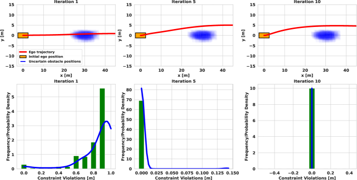
Figure 8: The top figure shows an ego-vehicle avoiding a uncertain static obstacles. The blue shaded region shows the uncertainty in the location of the obstacle. The trajectory in red depicts the output from Alg.2 at different iterations. The bottom figure shows the histogram of collision-constraint violation function $\overline{f}$ across iterations. We also fit a KDE to the histogram to approximately represent $p_{\overline{f}}$. As can be seen, $p_{\overline{f}}$ gradually converges to a Dirac-Delta distribution.

VI Validation and Benchmarking

This section aims to answer the following research questions

1. Q1: How is the sample efficiency of $r_{MMD}^{emp}$ as compared to CVaR and SAA estimate of collision constraint residual distribution? This is covered in Sections VI-C, VI-D, VI-E

2. Q2: What is the improvement in sample efficiency obtained by defining $r_{MMD}^{emp}$ over an optimal reduced-set as compared to randomly selected one? Refer to Section VI-F

3. Q3: What is the scalability of $r_{MMD}^{emp}$ based risk-aware trajectory optimization with respect to the number of obstacles (Section VI-G) ?

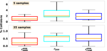
(a) Gaussian distribution

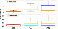
(b) Bimodal distribution

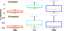
(c) Trimodal distribution

Figure 9: The figure shows the quantitative analysis(in the form of box plots) of collision rates achieved with different risk costs. We experiment with different types of obstacle trajectory distribution and for each type, we perform analysis across different sample sizes. In the case of Gaussian distribution (a), and $N^{^{\prime}}=5$, we observe that $r_{MMD}^{emp}$ leads to a worst-case collision-rate that is two times lower than that achieved using $r_{SAA}$. The performance gap between $r_{MMD}^{emp}$ and the other two baseline is more enhanced when the underlying obstacle trajectory distribution departs significantly from Gaussian. An example of this is show in (b) that is based on bimodal obstacle trajectory distribution. We observe that $r_{MMD}^{emp}$ leads to a worst-case collision-rate that is around five times lower than that achieved using $r_{CVaR}^{emp}$/$r_{SAA}$.

VI-A Implementation Details

We implemented our optimal reduced-set selection Alg.1 and Alg. 2 in Python using JAX [38] library as our GPU-accelerated linear algebra back-end. Our collision constraint function $f_{k}$ is designed assuming that the ego-vehicle and the obstacle are modeled as axis-aligned ellipses with size $(a_{1},a_{2})$. Thus, it has the following mathematical form

$$f_{k}:-\frac{(s_{k}-s_{o,k})^{2}}{a_{1}^{2}}-\frac{(d_{k}-d_{o,k})^{2}}{a_{2}^{2}}+1$$ (31)

where $\boldsymbol{\tau}_{k}=(s_{o,k},d_{o,k})$ is the position of the obstacle at time-step $k$ and is obtained from the trajectory predictor. Stacking $\boldsymbol{\tau}_{k}$ at different time steps give us $\boldsymbol{\tau}$.

The cost term $c$ in (5) has the following form

$$c(\mathbf{s}^{(q)},\mathbf{d}^{(q)})=c_{\theta}+c_{v}+c_{a}+c_{lane}$$ (32)

with

$$c_{\theta}=w_{\theta,1}\sum_{k}\max(0,|\theta_{k}|-\theta_{max})+w_{\theta,2}\theta^{2}_{k}+w_{\theta,3}\dot{\theta}^{2}_{k}+w_{\theta,4}\ddot{\theta}^{2}_{k},$$ (33)

The variable $\theta$ as defined earlier, is the steering angle and is a function of the the first and second derivatives of the position level trajectory ($q=\{1,2\}$) (recall eqn. (4)). The different $w_{\theta,i}$ are weights used to trade-off the effect of the cost terms with respect to each other. The derivatives of the $\theta_{k}$ are approximated through finite differencing.

The cost, $c_{v}$, $c_{a}$, $c_{lane}$ are defined as

$$c_{v}=\sum_{k}(\dot{s}_{k}-v_{des})^{2},c_{a}=\sum_{k}(\ddot{s}^{2}_{k}+\ddot{d}^{2}_{k}),c_{lane}=\sum_{k}(d_{k}-d_{des})^{2}$$ (34)

where $v_{des}$, $y_{des}$ is the desired longitudinal velocity and lane-offset to be tracked by the ego-vehicle.

The equality constraints $\mathbf{h}(\mathbf{s}^{(q)},\mathbf{d}^{(q)})=\mathbf{0}$ from (6) have the following components

$$(s_{0},\dot{s}_{0},\ddot{s}_{0})=(0,v_{x,init},a_{x,init}),$$ (35a)

$$(d_{0},\dot{d}_{0},\ddot{d}_{0},\dot{d}_{H})=(d_{init},v_{y,init},a_{y,init},0),$$ (35b)

where the r.h.s in (35a)-(35b) consists of the initial and terminal values of position variables and their derivatives along the axes of the Frenet-Frame.

The inequality constraints $\textbf{g}(\mathbf{s}^{(q)},\mathbf{d}^{(q)})\leq 0$ have the following components.

$$d_{min}\leq{d}_{k}\leq d_{max},\forall k$$ (36a)

$$\sqrt{\dot{s}_{k}^{2}+\dot{d}_{k}^{2}}\leq v_{max},\forall k$$ (36b)

$$\sqrt{\ddot{s}_{k}^{2}+\ddot{d}_{k}^{2}}\leq a_{max},\forall k$$ (36c)

The first inequality (36a) is the lane-boundary constraint. The parameters $(d_{min},d_{max})$ are defined with respect to the lane center-line or a reference path. The inequalities (36b)-(36c) bounds the magnitude of the velocity and acceleration respectively.

VI-A1 Benchmarking Environments

We consider the following collision avoidance scenarios for validating our approach as well as comparing against existing baselines.
Static Obstacles: We consider a two-lane driving scenario with static obstacles. We consider uncertainty in the location of the obstacles and three different choices for its underlying distribution: Gaussian distribution and Gaussian Mixture Model with two and three modes .

Dynamic Environments with Synthetic Trajectory Generator: In this benchmark, we consider a single dynamic obstacle whose future trajectory has two modes representing the different intents in its motions (e.g lane following or change, see Fig.10(a)). Moreover, we also consider uncertainty within the execution of each intent. We generate the trajectory distribution by sampling lane and desired velocity set-points from a discrete and a tri-modal GMM respectively, and passing them through the Frenet Space planner described in Appendix VIII-A.

NuScenes Dataset with Trajectron++ Predictor: In this benchmark, we consider the driving scenarios contained in the NuScenes [39] dataset. We use an off-the-shelf pre-trained trajectory predictor Trajectron++ [1] to generate obstacle trajectory distribution.

VI-A2 Baselines and Benchmarking Protocol

We compare our approach with two baselines obtained by just replacing our $r_{MMD}^{emp}$ with $r_{SAA}$ and $r_{CVaR}^{emp}$ in the trajectory optimizer of Alg.2. Our aim is to primarily compare the effectiveness of each risk cost at given sample size $N^{^{\prime}}$. Thus, to ensure that the planner biases has no influence on the result, we ensure that optimal trajectories resulting from the baselines and our approach indeed achieve zero risk cost. For example, optimal trajectory resulting from minimizing $r_{CVaR}^{emp}$ would achieve $r_{CVaR}^{emp}=0$ in all benchmarking examples. By adopting such a protocol, we facilitate explicitly comparing the finite-sample estimation error associated with each risk cost.

We split the sampled obstacle trajectories into two sets namely: optimization and validation set. The former set contains the trajectories from which we construct the $r_{MMD}^{emp}$ (including reduced-set computation), $r_{SAA}$ and $r_{CVaR}^{emp}$. The validation set trajectories are never seen by the planner. Moreover, the number of trajectories in validation set are at least two-orders of magnitude larger than the optimization set.

For our approach, we sample $100$ obstacle trajectories and then select $N^{^{\prime}}$ out of those as our reduced-set through Alg.1. We perform collision-checks along only $N^{^{\prime}}$ to estimate $r_{MMD}^{emp}$. Since $r_{SAA}$ and $r_{CVaR}^{emp}$ do not have any notion of reduced-set, we directly sample $N^{^{\prime}}$ obstacle trajectories to estimate their values.

VI-A3 Metrics

We primarily focus on the collision percentage on the validation set which is computed as follows. We check the computed optimal ego-trajectory for collision with each obstacle trajectory sample in the validation-set and divide the collision-free cases with the size of the validation set. We perform analysis for different sample size ($N^{^{\prime}}$) of the optimization set. Thus, implicitly $N^{^{\prime}}$ is also one of our comparison metric.

VI-B Qualitative Analysis of risk-aware planning with $r_{MMD}^{emp}$

Figure 8 shows the iteration-wise evolution of the optimal trajectory resulting from our optimizer in Alg.2 while using $r_{MMD}^{emp}$ as the collision risk cost. A static obstacle is placed at an arbitrary position and we introduce uncertainty by adding noise to its ground-truth position. As the iterations progress, the optimal trajectory shifts away from the potential obstacle locations making the trajectory increasingly safe. In the histogram plot of constraint violations, we observe that with each iteration, the probability of constraint violations goes down and by the $10^{th}$ iteration, the distribution $p_{\overline{f}}$ of the collision constraint violation function $\overline{f}$ has already converged to the Dirac delta distribution $p_{\delta}$.

VI-C Benchmarking in Synthetic Static Environments

In this benchmark, we randomly generated, 100 different obstacle configurations, each with 3 static obstacles. We introduced noise in the positions of all the obstacles. Three different types of noises were used: Gaussian, Bimodal GMM and Trimodal GMM. The initial position of the ego vehicle was fixed at the same value for all experiments. Similarly, the initial velocity of the ego vehicle was chosen as $3m/s$ in every experiment. We report the collision statistics(Number of collisions of the optimal trajectory with the obstacle samples from the validation set ( recall Sections VI-A2 and VI-A3 ).

We present the qualitative results in the complimentary video. The statistical benchmarking is presented in Fig.9. The following points are worth noting. First, the $r_{MMD}^{emp}$ trajectories show far lower number of collisions on the validation set than that computed using $r_{CVaR}^{emp}$ and $r_{SAA}$ risk costs at all sample sizes. For example, under Gaussian noise, $r_{MMD}^{emp}$ leads to a worst-case collision-rate that is two times lower than that achieved using $r_{SAA}$. Second, the difference in performance between $r_{MMD}^{emp}$ and $r_{CVaR}^{emp}$/$r_{SAA}$ becomes more stark as the underlying obstacle trajectories become increasingly more multi-modal. This showcases the ability of $r_{MMD}^{emp}$ to leverage RKHS embedding of distributions to capture the underlying probability distribution of obstacle trajectories and collision constraint residual function $p_{\overline{f}}$ with very few samples. Finally, $r_{MMD}^{emp}$ leads to fastest reduction in collision-rate with increase in sample size.

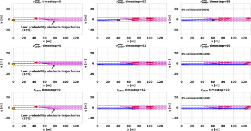
(a) In-lane driving scenario with low probability obstacle cut-in

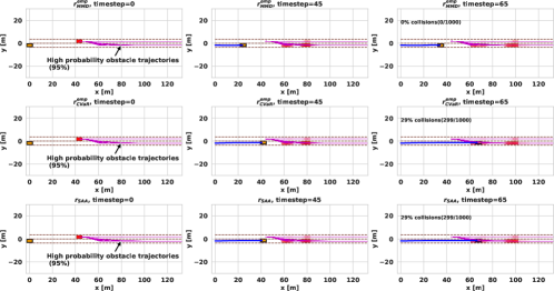
(b) In-lane driving scenario with high probability obstacle cut-in

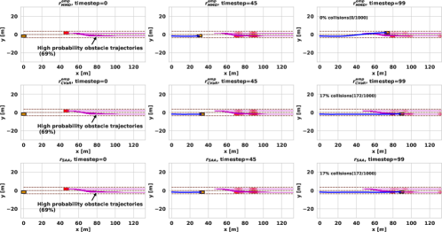
(c) Lane-change driving scenario with high probability obstacle cut-in

Figure 10: In (a)-(c) we synthetically generated scenarios where the obstacle cuts in the ego vehicle lane with varying probabilities. We show the maneuvers of the ego-vehicle computed using $N^{{}^{\prime}}=5$ obstacle trajectory samples. In (a)-(b), the ego-vehicle is required to respond to imminent collisions by just varying its speed. In contrast, the scenario in (c) allows the ego-vehicle to change lanes or overtake to avoid collisions. As can be seen, in low sample regime, in all the scenarios, only $r_{MMD}^{emp}$ is able to capture the true risk of the imminent collision and generate trajectories that have zero overlap between the ego-vehicle (yellow rectangle) and all the potential obstacle positions (red rectangles) over time.

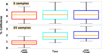
(a) In-lane driving scenario with low probability obstacle cut-in

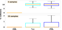
(b) In-lane driving scenario with high probability obstacle cut-in

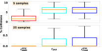
(c) Lane-change driving scenario with high probability obstacle cut-in

Figure 11: The box plots show the lower collision-rate achieved by minimizing $r_{MMD}^{emp}$ over the baseline risk cost $r_{SAA}$ and $r_{CVaR}^{emp}$ for the dynamic obstacle avoidance scenario of Fig.10, involving multi-modal obstacle trajectories.

VI-D Benchmarking in Synthetic Dynamic Environments

In this benchmark, we introduced a single dynamic obstacle with uncertain multi-modal future trajectory. As shown in Fig.10(a), the obstacle can either choose to stay in its lane or cut into the lane of the ego-vehicle, with the probability of the former being higher. In Fig.10(b), the situation is reverse and the obstacle is more likely to cut into the lane of the ego. In both the scenarios of Fig.10(a)-10(b), the ego-vehicle is constrained to move within its lane. In other words, it needs to either slow down or accelerate to avoid collision. We also consider a scenario in Fig.10(c) which is similar to 10(b), except in this case, the ego-vehicle can change-lane or overtake to avoid obstacles. In all these figures, we show the ego-vehicle rectangle in yellow and use red to show the obstacles. We plot all the potential obstacle positions over time to showcase the overlap between the ego-vehicle and obstacle footprints.

The quantitative results are summarized in Fig.11(a)-11(c). We once again observe that optimal trajectories obtained by minimizing $r_{MMD}^{emp}$ provides the best collision-avoidance performance across all sample-size $N^{^{\prime}}$. In particular, for the scenario shown in Fig.10(c) while using $N^{{}^{\prime}}=5$ obstacle trajectory samples, the median collision-rate achieved by minimizing $r_{MMD}^{emp}$ is 3 times lower than that resulting from $r_{CVaR}^{emp}$ and $r_{SAA}$. The performance difference shown in Fig.11(b), (observed for the scenario of Fig.10(b)), is even more stark with $r_{MMD}^{emp}$ demonstrating the zero collision on the validation set.

The qualitative results also show interesting trends, which when coupled with the quantitative results, demonstrate the ability of $r_{MMD}^{emp}$ to be safe without being overly conservative. In Fig.10(a)-10(b), only the $r_{MMD}^{emp}$ is able to capture the true risk of the imminent collision. Thus, the corresponding trajectories show the required de-acceleration. Interestingly, when the obstacle is more likely to merge into the ego-lane, minimizing $r_{MMD}^{emp}$ results in higher de-acceleration of the ego-vehicle. In contrast, $r_{CVaR}^{emp}$ and $r_{SAA}$ trajectories have higher speeds and they demonstrate collisions with some of the likely obstacle maneuvers. Finally, for the scenario of Fig.10(c), the $r_{MMD}^{emp}$ optimal trajectory correctly accounts for the likely lane-change behavior of the obstacle. As a result, the ego-vehicle moves into the adjacent lane that is more likely to be free. In contrast, $r_{CVaR}^{emp}$ and $r_{SAA}$ is unable to truly capture the likelihood of the obstacle lane-change intent and identify the lane-change possibility. As a result, the resulting trajectories are unable to leverage the likely free-space that is going to be created in the adjacent lane. Hence, $r_{CVaR}^{emp}$ and $r_{SAA}$ trajectories try to avoid collisions by just de-acceleration, which does not prove enough to ensure a very low collision rate.

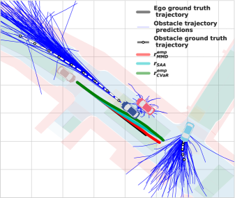
Figure 12: Risk-Aware trajectory planning in an unprotected intersection. The blue trajectories show the trajectory predictions of the neighboring vehicles. As can be seen, the predictions are highly multi-modal capturing different driving intents. Typical ego-vehicle trajectories resulting from different collision risk costs are also shown. It can be seen that $r_{MMD}^{emp}$ correctly understands that the cyan-vehicle is more likely to turn left. Hence, it shows least deviation from the recorded ground-truth (black), human-driven trajectory in the dataset. In contrast, $r_{CVaR}^{emp}$ and $r_{SAA}$ incorrectly puts more emphasis on the less likely scenario of cyan vehicle turning right. As a result, the resulting trajectories show a more deviation from the ground-truth trajectory.

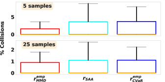
(a) Inlane scenario

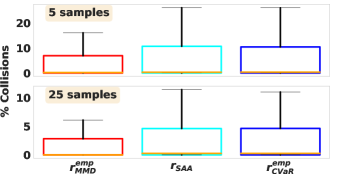
(b) Lane-change scenario

Figure 13: Comparing how well different risks $r_{MMD}^{emp}$, $r_{SAA}$, $r_{CVaR}^{emp}$ perform on real-world datasets with Neural Network based trajectory predictors (Trajectron++ [1] in this case). Typically, these predictors define a very complex distribution over the possible trajectories of the neighboring vehicles (obstacles). Hence, it is challenging to estimate the collision risk with a few predicted samples drawn from the distribution. As can be seen, our surrogate $r_{MMD}^{emp}$ leads to optimal trajectories with lowest collision-rate in both in-lane driving and lane-change scenarios.

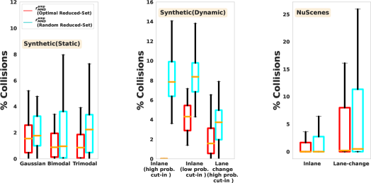
Figure 14: Comparison of collision-rate achieved by minimizing $r_{MMD}^{emp}$ constructed with the optimal and random reduced-set of size $N^{^{\prime}}=5$. The former set-up leads to safer trajectories with a significantly better median and worst-case statistics. The difference is particularly stark when the obstacle trajectory distribution departs significantly from a Gaussian.

VI-E Benchmarking On NuScenes Dataset Using Trajectron++ Predictor

We evaluated a total of 160 scenes in this dataset. Each scene comes with a reference center-line and a designated ego vehicle. Any vehicle other than the ego was treated as an obstacle. A typical scene is shown in Fig.12. We considered two setting namely in-lane driving and lane-change. In the former, the ego-vehicle needs to avoid collisions by just changing the speed, while the latter allows for the full set of maneuvers to the ego-vehicle. We report the collision statistics in Fig. 13. We used Trajectron++ [1] as a deep neural network based trajectory predictor. We observed that for both scenarios(in-lane and lane-change), our approach based on $r_{MMD}^{emp}$ has the lowest worst-case collision-rate among all the approaches. The improvement is approximately two-times in the lane-change scenario when using $N^{^{\prime}}=25$ samples from obstacle trajectory distribution. The median collision-rate for our approach and the baselines were zero.

A typical example of trajectories obtained in this benchmark is shown in Fig.12 which demonstrates an unprotected intersection. The predicted trajectories cover multi-modal intents (e.g turn left or right). The trajectories resulting from minimizing $r_{MMD}^{emp}$ is closest to the ground-truth (human-driven) recorded trajectory in the same scenario. This in turn can be attributed to the ability to $r_{MMD}^{emp}$ to correctly identify (through its reduced-set, recall Fig.7 ) the more likely maneuvers. For example, consider the cyan obstacle/vehicle. The predicted trajectories cover both left and right turns. But the ground-truth motion for the obstacle is the left turn maneuver and $r_{MMD}^{emp}$ is able to correctly give more importance to left-turn predictions. In contrast, the $r_{SAA}$, $r_{CVaR}^{emp}$ show overly conservative maneuver driven by the trajectory samples that predict right-turn for the cyan obstacle.

VI-F Ablation Results

Fig.14 performs an ablation when instead of using Alg.1, we form the reduced-set by random sub-selection (recall Section IV-C1). It can be seen that constructing $r_{MMD}^{emp}$ on the optimal reduced-set leads to lower collision-rate across all scenes. The difference between the random and the optimal variant is particularly stark when the underlying trajectory distribution is much more complex than a Gaussian. Moreover, the variance in the collision-rate across the benchmarking scenes is lower when using the optimal reduced-set.

VI-G Computation Time

Table I shows the computation time required for our reduced-set optimization Alg.1 and Alg.2 for different sample sizes on an RTX 3090 Desktop with 16 GB RAM. We report the timing separately for Alg.1 and 2. The former depends on the number of obstacles and also on the size of the optimal reduced-set ($N^{^{\prime}}$) that we want to construct. At any given $N^{^{\prime}}$, Alg.1 show almost linear growth in the computation-time with respect to the number of obstacles. However, once Alg.1 is done, the subsequent computation of estimating $r_{MMD}^{emp}$ for a given ego-vehicle trajectory can be suitably parallelized. Hence the increase in computation-time for Alg.2 with respect to the number of obstacles is very minimal.

VII Conclusions and Future Work

Estimating and minimizing collision risk based on predicted obstacle trajectories is one of the fundamental problems in autonomous driving. Existing works have used techniques like SAA ($r_{SAA}$, Eqn. 11) and CVaR ($r_{CVaR}^{emp}$, Eqn.12) estimate of collision constraint residual function (recall (10)) to define a risk surrogate conditioned on the ego-vehicle and obstacle trajectories. Although effective, one of the key limitation with these two risk estimation techniques is that there exists no systematic way of maximizing their effectiveness at a given finite sample size. To fill this gap, we proposed to use the MMD between the distribution of collision-constraint residuals and the Dirac-Delta distribution to model collision risk ($r_{MMD}^{emp}$, Eqn.23).

The choice of our risk surrogate allows us to use the notion of reduced-set to maximize its effectiveness at a given sample size. Put differently, reduced-set allows us to choose only a subset of predicted obstacle trajectories to formulate our risk surrogate while incurring minimal loss in its accuracy. However, to fully leverage its power, we need to go beyond the existing convention of constructing reduced-set by random sub-selection [11] from a larger sample set. With this motivation, we proposed for the first time, a bi-level optimization that constructs reduced-set in a way that ensures minimal loss in downstream risk estimation. As a by product, the bi-level optimizer also provides an optimal kernel parameter.

We compared the effectiveness of $r_{MMD}^{emp}$, $r_{SAA}$, and $r_{CVaR}^{emp}$ when used as a risk-cost in a trajectory optimization. We showed that $r_{MMD}^{emp}$ provides substantially improved performance, especially at lower sample sizes. The performance improvement is particularly impressive when the underlying prediction distribution departs substantially from a Gaussian. Our results demonstrates the suitability of $r_{MMD}^{emp}$ to be used alongside large Neural Networks based predictors that induces unknown/intractable distribution over obstacle trajectories. We also demonstrated preliminary results to this end on the driving scenes from the NuScenes dataset [39] using Trajectron++ as our trajectory predictor.

Our approach is not limited to autonomous driving and our future efforts are focused towards extending it to 3D navigation of drones and manipulation in cluttered environments. We are also looking to extend our MMD-based risk surrogate to modeling collision risk under uncertain vehicle dynamics.

TABLE I: Computation Time(in seconds) vs Number of Reduced-set samples

	Number of obstacles
Number of Reduced-set samples	1 obs. (Alg. 1/Alg.2)	2 obs. (Alg. 1/Alg.2)	3 obs. (Alg. 1/Alg.2)
5 samples	0.005/0.01	0.01/0.01	0.016/0.01
10 samples	0.006/0.01	0.012/0.01	0.019/0.01
20 samples	0.006/0.01	0.012/0.01	0.017/0.01
30 samples	0.007/0.01	0.014/0.01	0.02/0.01
40 samples	0.007/0.01	0.014/0.01	0.02/0.01
50 samples	0.008/0.01	0.015/0.01	0.023/0.01

VIII Appendix

VIII-A Frenet Planner

Let $\mathbf{b}=(b_{d},b_{v})$ be the lateral offset and desired velocity setpoints. Our Frenet planner inspired from [25] boils down to solving the following trajectory optimization.

$$\min\sum_{k}c_{s}+c_{l}+c_{v}$$ (37a)

$$\mathbf{h}(\mathbf{s}^{(q)},\mathbf{d}^{(q)})=\mathbf{0}$$ (37b)

$$c_{s}(\ddot{s}_{k},\ddot{d}_{k})=\ddot{s}^{2}_{k}+\ddot{d}^{2}_{k}$$ (38a)

$$c_{l}(d_{k},\dot{d}_{k},\ddot{d}_{k})=(\ddot{d}_{k}-\kappa_{p}(d_{k}-b_{d})-\kappa_{v}\dot{d}_{k})^{2}$$ (38b)

$$c_{v}(\dot{s}_{k},\ddot{s}_{k})=(\ddot{s}_{k}-\kappa_{p}(\dot{s}_{k}-b_{v}))^{2}$$ (38c)

The first term $c_{s}(.)$ in the cost function (37a) ensures smoothness in the planned trajectory by penalizing high accelerations at discrete time instants. The last two terms ($c_{l}(.),c_{v}(.)$) model the tracking of lateral offset ($b_{d}$) and forward velocity $(b_{v})$ set-points respectively with gain $(\kappa_{p},\kappa_{v})$. The above optimization is an equality constrained QP that have a closed-form solution.

VIII-B Simplification of $r_{MMD}^{emp}$ Based On Kernel Trick

We expand equation (23) in the following manner

$$\left\|\widehat{\mu}[\overline{f^{^{\prime}}}]-\widehat{\mu}[\delta]\right\|_{\mathcal{H}}^{2}=\langle\widehat{\mu}[\overline{f^{^{\prime}}}],\widehat{\mu}[\overline{f^{^{\prime}}}]\rangle-2\langle\widehat{\mu}[\overline{f^{^{\prime}}}],\widehat{\mu}[\delta]\rangle+\langle\widehat{\mu}[\delta],\widehat{\mu}[\delta]\rangle$$ (39)

Substituting RKHS embeddings of $\overline{f^{^{\prime}}}$ (25) and $\delta\sim p_{\delta}$ in (39)

$$\langle\widehat{\mu}[\overline{f^{^{\prime}}}],\widehat{\mu}[\overline{f^{^{\prime}}}]\rangle =\langle\sum_{i=1}^{N^{^{\prime}}}{{}^{i}}\beta K(^{i}\overline{f^{^{\prime}}},\cdot),\sum_{j=1}^{N^{^{\prime}}}{{}^{j}}\beta K(^{j}\overline{f^{^{\prime}}},\cdot)\rangle$$ (40a)

$$\langle\widehat{\mu}[\overline{f^{^{\prime}}}],\widehat{\mu}[\delta]\rangle =\langle\sum_{i=1}^{N^{^{\prime}}}{{}^{i}}\beta K(^{i}\overline{f^{^{\prime}}},\cdot),\frac{1}{N^{^{\prime}}}\sum_{j=1}^{N^{{}^{\prime}}}K(^{j}\delta,\cdot)\rangle$$ (40b)

$$\langle\widehat{\mu}[\delta],\widehat{\mu}[\delta]\rangle =\langle\frac{1}{N^{^{\prime}}}\sum_{i=1}^{N^{{}^{\prime}}}K(^{i}\delta,\cdot),\frac{1}{N^{^{\prime}}}\sum_{j=1}^{N^{^{\prime}}}K(^{j}\delta,\cdot)\rangle$$ (40c)

where the computations are done over the reduced-set introduced in Section IV-C. Substituting (40) in (39) and using the kernel trick introduced in Section III-A, we can now derive an optimization friendly expression for the r.h.s of (23) as follows

$$\left\|\widehat{\mu}[\overline{f^{^{\prime}}}]-\widehat{\mu}[\delta]\right\|_{2}^{2}=\mathbf{C}_{\beta}\mathbf{K}_{\overline{f^{^{\prime}}},\overline{f^{^{\prime}}}}\mathbf{C}_{\beta}^{\intercal}-2\mathbf{C}_{\beta}\mathbf{K}_{\overline{f^{^{\prime}}},\delta}\mathbf{C}_{\overline{\beta}}^{\intercal}+\mathbf{C}_{\overline{\beta}}\mathbf{K}_{\delta,\delta}\mathbf{C}_{\overline{\beta}}^{\intercal}$$ (41)

where $\mathbf{C}_{\beta}$ and $\mathbf{C}_{\overline{\beta}}$ are weight vectors given by

$$\mathbf{C}_{\beta}=\left[{{}^{1}}\beta,{{}^{2}}\beta,\dots,{{}^{N^{^{\prime}}}}\beta\right],\mathbf{C}_{\overline{\beta}}=\left[\frac{1}{N^{^{\prime}}},\frac{1}{N^{^{\prime}}},\dots,\frac{1}{N^{^{\prime}}}\right]$$

and $\mathbf{K}_{\overline{f^{^{\prime}}},\overline{f^{^{\prime}}}},\mathbf{K}_{\overline{f^{^{\prime}}},\delta}$ and $\mathbf{K}_{\delta,\delta}$ are kernel matrices defined as

$$\mathbf{K}_{\overline{f^{^{\prime}}},\overline{f^{^{\prime}}}} =\begin{bmatrix}K(^{1}\overline{f^{^{\prime}}},^{1}\overline{f^{^{\prime}}})&\dots&K(^{1}\overline{f^{^{\prime}}},^{N^{^{\prime}}}\overline{f^{^{\prime}}})\\ K(^{2}\overline{f^{^{\prime}}},^{1}\overline{f^{^{\prime}}})&\dots&K(^{2}\overline{f^{^{\prime}}},^{N^{^{\prime}}}\overline{f^{^{\prime}}})\\ \vdots&\ddots&\vdots\\ K(^{N^{^{\prime}}}\overline{f^{^{\prime}}},^{1}\overline{f^{^{\prime}}})&\dots&K(^{N^{^{\prime}}}\overline{f^{^{\prime}}},^{N^{^{\prime}}}\overline{f^{^{\prime}}})\end{bmatrix}$$

$$\mathbf{K}_{\overline{f^{^{\prime}}},\delta} =\begin{bmatrix}K(^{1}\overline{f^{^{\prime}}},0)&\dots&K(^{1}\overline{f^{^{\prime}}},0)\\ K(^{2}\overline{f^{^{\prime}}},0)&\dots&K(^{2}\overline{f^{^{\prime}}},0)\\ \vdots&\ddots&\vdots\\ K(^{N^{^{\prime}}}\overline{f^{^{\prime}}},0)&\dots&K(^{N^{^{\prime}}}\overline{f^{^{\prime}}},0)\end{bmatrix},\mathbf{K}_{\delta,\delta} =\mathbf{1}_{N^{^{\prime}}\times N^{^{\prime}}}$$

References

- [1] B. Ivanovic and M. Pavone, “The trajectron: Probabilistic multi-agent trajectory modeling with dynamic spatiotemporal graphs,” in Proceedings of the IEEE/CVF International Conference on Computer Vision, 2019, pp. 2375–2384.
- [2] A. Gupta, J. Johnson, L. Fei-Fei, S. Savarese, and A. Alahi, “Social gan: Socially acceptable trajectories with generative adversarial networks,” in Proceedings of the IEEE conference on computer vision and pattern recognition, 2018, pp. 2255–2264.
- [3] N. Lee, W. Choi, P. Vernaza, C. B. Choy, P. H. Torr, and M. Chandraker, “Desire: Distant future prediction in dynamic scenes with interacting agents,” in Proceedings of the IEEE conference on computer vision and pattern recognition, 2017, pp. 336–345.
- [4] T. M. Roddenberry, N. Glaze, and S. Segarra, “Principled simplicial neural networks for trajectory prediction,” 2021. [Online]. Available: https://arxiv.org/abs/2102.10058
- [5] S. Zamboni, Z. T. Kefato, S. Girdzijauskas, C. Norén, and L. Dal Col, “Pedestrian trajectory prediction with convolutional neural networks,” Pattern Recognition, vol. 121, p. 108252, 2022. [Online]. Available: https://www.sciencedirect.com/science/article/pii/S0031320321004325
- [6] C. Xu, M. Li, Z. Ni, Y. Zhang, and S. Chen, “Groupnet: Multiscale hypergraph neural networks for trajectory prediction with relational reasoning,” in Proceedings of the IEEE/CVF Conference on Computer Vision and Pattern Recognition (CVPR), June 2022, pp. 6498–6507.
- [7] H. Zhu and J. Alonso-Mora, “Chance-constrained collision avoidance for mavs in dynamic environments,” IEEE Robotics and Automation Letters, vol. 4, no. 2, pp. 776–783, 2019.
- [8] L. Blackmore, M. Ono, and B. C. Williams, “Chance-constrained optimal path planning with obstacles,” IEEE Transactions on Robotics, vol. 27, no. 6, pp. 1080–1094, 2011.
- [9] M. Castillo-Lopez, P. Ludivig, S. A. Sajadi-Alamdari, J. L. Sanchez-Lopez, M. A. Olivares-Mendez, and H. Voos, “A real-time approach for chance-constrained motion planning with dynamic obstacles,” IEEE Robotics and Automation Letters, vol. 5, no. 2, pp. 3620–3625, 2020.
- [10] C. Dawson, A. Jasour, A. Hofmann, and B. Williams, “Provably safe trajectory optimization in the presence of uncertain convex obstacles,” in 2020 IEEE/RSJ International Conference on Intelligent Robots and Systems (IROS), 2020, pp. 6237–6244.
- [11] C.-J. Simon-Gabriel, A. Scibior, I. O. Tolstikhin, and B. Schölkopf, “Consistent kernel mean estimation for functions of random variables,” Advances in Neural Information Processing Systems, vol. 29, 2016.
- [12] A. Gretton, K. M. Borgwardt, M. J. Rasch, B. Schölkopf, and A. Smola, “A kernel two-sample test,” J. Mach. Learn. Res., vol. 13, no. null, p. 723–773, 2012.
- [13] B. K. Pagnoncelli, S. Ahmed, and A. Shapiro, “Sample average approximation method for chance constrained programming: theory and applications,” Journal of optimization theory and applications, vol. 142, no. 2, pp. 399–416, 2009.
- [14] J. Yin, Z. Zhang, and P. Tsiotras, “Risk-aware model predictive path integral control using conditional value-at-risk,” 2022. [Online]. Available: https://arxiv.org/abs/2209.12842
- [15] A. Liniger and L. van Gool, “Safe motion planning for autonomous driving using an adversarial road model,” 2020.
- [16] S. S. Harithas, R. D. Yadav, D. Singh, A. K. Singh, and K. M. Krishna, “Cco-voxel: Chance constrained optimization over uncertain voxel-grid representation for safe trajectory planning,” in 2022 International Conference on Robotics and Automation (ICRA). IEEE, 2022, pp. 11 087–11 093.
- [17] Y. Shirai, D. K. Jha, and A. U. Raghunathan, “Covariance steering for uncertain contact-rich systems,” in 2023 IEEE International Conference on Robotics and Automation (ICRA). IEEE, May 2023. [Online]. Available: http://dx.doi.org/10.1109/ICRA48891.2023.10160249
- [18] T. Lew, R. Bonalli, and M. Pavone, “Risk-averse trajectory optimization via sample average approximation,” IEEE Robotics Autom. Lett., vol. 9, no. 2, pp. 1500–1507, 2024. [Online]. Available: https://doi.org/10.1109/LRA.2023.3331889
- [19] A. Shapiro, D. Dentcheva, and A. Ruszczynski, Lectures on Stochastic Programming: Modeling and Theory, Second Edition, ser. MOS-SIAM Series on Optimization. Society for Industrial and Applied Mathematics, 2014. [Online]. Available: https://books.google.ee/books?id=ob4ABAAAQBAJ
- [20] K. Muandet, K. Fukumizu, B. Sriperumbudur, and B. Schölkopf, “Kernel mean embedding of distributions: A review and beyond,” Foundations and Trends® in Machine Learning, vol. 10, no. 1–2, p. 1–141, 2017. [Online]. Available: http://dx.doi.org/10.1561/2200000060
- [21] B. Schölkopf, J. Platt, and T. Hofmann, “A kernel method for the two-sample-problem,” 2007.
- [22] Z. I. Botev, D. P. Kroese, R. Y. Rubinstein, and P. L’Ecuyer, “The cross-entropy method for optimization,” in Handbook of statistics. Elsevier, 2013, vol. 31, pp. 35–59.
- [23] G. Williams, P. Drews, B. Goldfain, J. M. Rehg, and E. A. Theodorou, “Aggressive driving with model predictive path integral control,” in 2016 IEEE International Conference on Robotics and Automation (ICRA). IEEE, 2016, pp. 1433–1440.
- [24] M. Bhardwaj, B. Sundaralingam, A. Mousavian, N. D. Ratliff, D. Fox, F. Ramos, and B. Boots, “Storm: An integrated framework for fast joint-space model-predictive control for reactive manipulation,” in Conference on Robot Learning. PMLR, 2022, pp. 750–759.
- [25] J. Wei, J. M. Snider, T. Gu, J. M. Dolan, and B. Litkouhi, “A behavioral planning framework for autonomous driving,” in 2014 IEEE Intelligent Vehicles Symposium Proceedings. IEEE, 2014, pp. 458–464.
- [26] H. Masnavi, J. Shrestha, M. Mishra, P. Sujit, K. Kruusamäe, and A. K. Singh, “Visibility-aware navigation with batch projection augmented cross-entropy method over a learned occlusion cost,” IEEE Robotics and Automation Letters, vol. 7, no. 4, pp. 9366–9373, 2022.
- [27] V. K. Adajania, A. Sharma, A. Gupta, H. Masnavi, K. M. Krishna, and A. K. Singh, “Multi-modal model predictive control through batch non-holonomic trajectory optimization: Application to highway driving,” IEEE Robotics and Automation Letters, vol. 7, no. 2, pp. 4220–4227, 2022.
- [28] G. C. Calafiore and M. C. Campi, “The scenario approach to robust control design,” IEEE Transactions on automatic control, vol. 51, no. 5, pp. 742–753, 2006.
- [29] G. C. Calafiore and L. Fagiano, “Robust model predictive control via scenario optimization,” IEEE Transactions on Automatic Control, vol. 58, no. 1, pp. 219–224, 2012.
- [30] H. Ahn, C. Chen, I. M. Mitchell, and M. Kamgarpour, “Safe motion planning against multimodal distributions based on a scenario approach,” IEEE Control Systems Letters, vol. 6, pp. 1142–1147, 2022.
- [31] D. Bernardini and A. Bemporad, “Scenario-based model predictive control of stochastic constrained linear systems,” in Proceedings of the 48h IEEE Conference on Decision and Control (CDC) held jointly with 2009 28th Chinese Control Conference, 2009, pp. 6333–6338.
- [32] G. Schildbach, L. Fagiano, C. Frei, and M. Morari, “The scenario approach for stochastic model predictive control with bounds on closed-loop constraint violations,” Automatica, vol. 50, no. 12, pp. 3009–3018, 2014. [Online]. Available: https://www.sciencedirect.com/science/article/pii/S0005109814004166
- [33] J.-J. Zhu, B. Schoelkopf, and M. Diehl, “A kernel mean embedding approach to reducing conservativeness in stochastic programming and control,” in Learning for Dynamics and Control. PMLR, 2020, pp. 915–923.
- [34] K. A. Mustafa, D. J. Ornia, J. Kober, and J. Alonso-Mora, “Racp: Risk-aware contingency planning with multi-modal predictions,” IEEE Transactions on Intelligent Vehicles, 2024.
- [35] Y. Nemmour, H. Kremer, B. Schölkopf, and J.-J. Zhu, “Maximum mean discrepancy distributionally robust nonlinear chance-constrained optimization with finite-sample guarantee,” in 2022 IEEE 61st Conference on Decision and Control (CDC). IEEE, 2022, pp. 5660–5667.
- [36] B. Sharma, A. Sharma, K. M. Krishna, and A. K. Singh, “Hilbert space embedding-based trajectory optimization for multi-modal uncertain obstacle trajectory prediction,” in 2023 IEEE/RSJ International Conference on Intelligent Robots and Systems (IROS). IEEE, 2023, pp. 7448–7455.
- [37] B. Gopalakrishnan, A. K. Singh, K. M. Krishna, and D. Manocha, “Solving chance-constrained optimization under nonparametric uncertainty through hilbert space embedding,” IEEE Transactions on Control Systems Technology, vol. 30, no. 3, pp. 901–916, 2021.
- [38] J. Bradbury, R. Frostig, P. Hawkins, M. J. Johnson, C. Leary, D. Maclaurin, G. Necula, A. Paszke, J. VanderPlas, S. Wanderman-Milne, and Q. Zhang, “JAX: composable transformations of Python+NumPy programs,” 2018. [Online]. Available: http://github.com/google/jax
- [39] H. Caesar, V. Bankiti, A. H. Lang, S. Vora, V. E. Liong, Q. Xu, A. Krishnan, Y. Pan, G. Baldan, and O. Beijbom, “nuscenes: A multimodal dataset for autonomous driving,” in Proceedings of the IEEE/CVF conference on computer vision and pattern recognition, 2020, pp. 11 621–11 631.