Analyzing Practical Policies for Multiresource Job Scheduling

Abstract.

Modern cloud computing workloads are composed of multiresource jobs that require a variety of computational resources in order to run, such as CPU cores, memory, disk space, or hardware accelerators. A single cloud server can typically run many multiresource jobs in parallel, but only if the server has sufficient resources to satisfy the demands of every job. A scheduling policy must therefore select sets of multiresource jobs to run in parallel in order to minimize the mean response time across jobs — the average time from when a job arrives to the system until it is completed. Unfortunately, achieving low response times by selecting sets of jobs that fully utilize the available server resources has proven to be a difficult problem.

In this paper, we develop and analyze a new class of policies for scheduling multiresource jobs, called Markovian Service Rate (MSR) policies. While prior scheduling policies for multiresource jobs are either highly complex to analyze or hard to implement, our MSR policies are simple to implement and are amenable to response time analysis. We show that the class of MSR policies is throughput-optimal in that we can use an MSR policy to stabilize the system whenever it is possible to do so. We also derive bounds on the mean response time under an MSR algorithm that are tight up to an additive constant. These bounds can be applied to systems with different preemption behaviors, such as fully preemptive systems, non-preemptive systems, and systems that allow preemption with setup times. We show how our theoretical results can be used to select a good MSR policy as a function of the system arrival rates, job service requirements, the server’s resource capacities, and the resource demands of the jobs.

1. Introduction

Modern data center servers include a wide variety of computational resources, including CPU cores, network cards, local or disaggregated memory and storage, and specialized accelerators such as GPUs. Each job request in the data center requires some set of diverse resources in order to run, such as a few CPU cores, some amount of memory, some amount of storage (Maguluri and Srikant, 2013; Maguluri et al., 2014; Tirmazi et al., 2020). Each job also has an associated service requirement, which describes how long the job must run once it has been allocated its requested resources. Because a single job requires several types of resources, we refer to these jobs as multiresource jobs. To serve multiresource jobs quickly, a single server generally aims to run many multiresource jobs in parallel. However, the server also has a limited capacity for each resource. Hence, a set of multiresource jobs can only be run in parallel if their aggregate demand for each resource is less than the server’s capacity for that resource. For example, in order to run some set of jobs concurrently, the number of total CPU cores demanded by the jobs should not exceed the total number of CPU cores in the server, and the total memory required by these jobs should not exceed the DRAM capacity of the server. This raises the question of how a scheduling policy should choose sets of multiresource jobs to run in parallel on a data center server.

When scheduling multiresource jobs, the goal is often to reduce job response times, the time from when a job arrives to the system until it is completed (Tirmazi et al., 2020; Delimitrou and Kozyrakis, 2014). In particular, this paper considers the problem of designing scheduling policies to minimize mean response time, the long-run average response time across a stream of arriving multiresource jobs. Unfortunately, optimizing the response times of multiresource jobs has proven to be difficult (Harchol-Balter, 2022; Ghaderi, 2016a; Maguluri and Srikant, 2013; Stolyar, 2004). Much of the literature on multiresource jobs has been devoted to proving system stability results (Maguluri et al., 2014; Ghaderi, 2016a), while response time analysis has been largely restricted to simple policies such as First-Come-First-Served (FCFS) that perform poorly in practice (Grosof et al., 2023). Furthermore, many existing results on scheduling multiresource jobs suggest using a MaxWeight policy (Maguluri et al., 2014) that is too complex to efficiently implement in a real system. As a result, modern data centers are generally greatly overprovisioned in order to achieve low response times (Tirmazi et al., 2020), and rely on heuristic scheduling policies, such as BackFilling policies like First-Fit, that admit no theoretical analysis or guarantees (Grosof et al., 2022).

This paper introduces a new class of policies for scheduling multiresource jobs called Markovian Service Rate (MSR) policies. We prove strong stability results for this class of policies and bounds on mean response time. Using these bounds, we derive an accurate approximation of the mean response time of an MSR policy. Best of all, our MSR policies require a single offline optimization step, after which the policy runs in constant time per scheduling decision.

1.1. The Problem: Scheduling to Reduce Wastage

The key challenge in scheduling multiresource jobs is that it is difficult to fully utilize all the server resources at all times. Intuitively, finding sets of jobs that fully utilize all server resources requires solving some type of bin-packing problem, and as a result, naïve scheduling policies can greatly underutilize the available system resources. We describe the average amount of idle resources under a given scheduling policy as the wastage of the policy. In general, high wastage leads to higher mean response time, and possibly even instability.

To illustrate this problem, we consider the FCFS policy for multiresource jobs described in (Grosof et al., 2023). Whenever a job arrives or departs the system, FCFS repeatedly examines the job at the front of the queue and puts the job in service as long as the server has enough of resources to accommodate it. This process continues until either the queue is empty or the next job in the queue would exceed the server’s capacity for one or more resources. Although it is a simple, intuitive policy, FCFS can greatly underutilize the available system resources. For example, consider the case where the arriving jobs alternate between requesting 4 and 2 CPU cores, each job must run for one second, and the server has 8 CPU cores in total. In this case, FCFS grabs a 4-core job and a 2-core job from the front of the queue. The next job requires four cores, but only two are available, so the remaining two cores in the server will be idle. Hence, in our example, FCFS always wastes at least two cores and completes at most two jobs per second. Alternatively, consider a no-wastage policy that alternates between running four 2-core jobs together or two 4-core jobs together. We can see that this no-wastage policy can complete up to three jobs per second. As a result, the capacity region of the no-wastage policy dominates that of FCFS. We formalize this argument in Section 4.

FCFS suffers here because its high wastage limits the number of jobs that can be run in parallel. While it is easy to spot better packings than FCFS in this simple example, the complexity of finding low-wastage allocations explodes as the number of job types grows (e.g., if some jobs requested three cores) and as the number of resource types grows (e.g., jobs request CPUs, GPUs, and DRAM).

1.2. Our Goal: Improved Low-complexity Scheduling Policies

To avoid the pitfalls of an FCFS-style policy, the canonical work on scheduling multiresource jobs suggests finding low-wastage allocations by solving complex bin-packing problems repeatedly to continuously determine the next scheduler action (Stolyar, 2004; Maguluri et al., 2014). These are the so-called MaxWeight algorithms that have been shown to maximize the capacity regions of the system (i.e., throughput optimality) and achieve empirically low mean response time. Unfortunately, running MaxWeight algorithms in real systems is impractical due to the complexity of the bin-packing problem that must be solved repeatedly. MaxWeight also preempts jobs frequently, which may not be feasible in all systems. It is a long-standing open problem to find and analyze policies that are both simple enough to run in practice, but still achieve low mean response time similar to a MaxWeight policy.

The closest the scheduling community has come to solving this problem is the Randomized-Timers approach of (Ghaderi, 2016a), which describes a non-preemptive policy for scheduling multiresource jobs that can compute each scheduling decision with low complexity (complexity is linear in the number of job types). Randomized-Timers is throughput-optimal, but the policy often results in high mean response time compared to MaxWeight. Additionally, the Randomized-Timers algorithm is a complicated randomized algorithm and there is no analysis of its mean response time.

Our goal in this paper is to develop policies with the best features of MaxWeight and Randomized-Timers. That is, we seek low-complexity policies that can achieve low mean response time under a variety of job preemption models. Our policies should maximize the capacity region of the system, and be accompanied by strong theoretical guarantees about mean response time.

Policy	Throughput Optimal	Low Complexity	Mean Response Time Analysis	Preemption Model
FCFS (Grosof et al., 2023)		x	x	non-preemptive
First-Fit (Grosof et al., 2022)		x		non-preemptive
ServerFilling (Grosof et al., 2022)	Sometimes	x	Sometimes	preemptive
MaxWeight (Maguluri et al., 2014)	x		Heavy traffic	preemptive
Randomized-Timers (Psychas and Ghaderi, 2018)	x	x		non-preemptive
MSR	x	x	x	general

Table 1. Comparison of MSR policies to other multiresource job scheduling policies.

1.3. Our Solution: MSR Scheduling Policies

The main contribution of this paper is the analysis of the Markovian Service Rate (MSR) class of policies for scheduling multiresource jobs. MSR policies use a finite-state Continuous Time Markov Chain (CTMC) to determine which set of jobs to run at every moment in time. The states of this CTMC, known as the candidate set of possible scheduling actions, as well as its transition rates, are determined offline via a one-time optimization step that considers the service requirements distributions and arrival rate for a given workload. We prove that an MSR policy can achieve low mean response time without the computational complexity of MaxWeight by deriving mean response time bounds that are additively tight. We also use our bounds to derive a mean response time approximation for MSR policies that is shown to be highly accurate in simulation. We show how to select an MSR policy that also stabilizes the system whenever it’s possible to do so.

Our analysis generalizes to a variety of job preemption models. We consider the cases where jobs are fully preemptible, where jobs are non-preemptible, and where job preemptions are accompanied by setup times. In each case, we show how to select an appropriate MSR policy and analyze the mean response time under this policy. Specifically, the contributions of the paper are as follows:

• First, in Section 4, we introduce the class of MSR scheduling policies for multiresource jobs. These policies are easy to implement with low computational complexity. We show that, under a variety of job preemption behaviors, there exists an MSR policy that can stabilize the system whenever it is possible to do so. Hence, we say that the class of MSR policies is throughput-optimal under each preemption behavior.

• Next, in Section 5, we analyze the mean response time of the multiresource job system under any MSR policy by decoupling the system into a set of $M/M/1$ Markovian Modulated Service Rate systems. By analyzing these decoupled problems, we prove additively tight bounds on the mean queue length of an MSR policy.

• In Section 6, we show how our theoretical results can be used to choose an MSR policy with good mean response time under a variety of job preemption behaviors.

• Section 7 validates our policy choices by comparing MSR policies to a variety of policies from the literature in theory and in simulation. We find that our MSR policies are competitive with these other policies, while also being analytically tractable and simple to implement.

Table 1 compares our new MSR policies to existing policies for scheduling multiresource jobs.

2. Prior Work

Scheduling in Real-world Systems. Multiresource jobs are ubiquitous in datacenters and supercomputing centers where each job requires some amount of several different resources (e.g., CPUs, GPUs, memory, disk space, network bandwidth) in order to run. As a result, the systems community has extensively considered the problem of scheduling multiresource jobs (Verma et al., 2015; Tirmazi et al., 2020; Delimitrou and Kozyrakis, 2014; Lipari, 2012; SchedMD, 2021; Hindman et al., 2011). Unfortunately, almost all of this work depends on a complex set of heuristic scheduling policies that do not provide theoretical performance guarantees.

The Multiserver Job Model. Prior theoretical work has considered the multiserver job model (Harchol-Balter, 2022) where each job demands multiple servers in order to run. Several papers have developed throughput-optimal policies for this multiserver job system, such as the MaxWeight Policy (Maguluri and Srikant, 2013) and the Randomized-Timers policy (Ghaderi, 2016a). However, neither of these policies emit a general analysis of mean response time.

Other work (Grosof et al., 2020; Weina Wang and Harchol-Balter, 2021; Grosof et al., 2022) has analyzed the multiserver job system in a variety of special cases such as restricting jobs to belong to one of two classes (Grosof et al., 2020), considering the system in a variety of scaling limits (Weina Wang and Harchol-Balter, 2021), and requiring job server demands to be powers-of-2 (Grosof et al., 2022). In these special cases, the analysis relies heavily on the fact that there is only one resource type, servers.

The Multiresource Job Model. The multiresource job model is a generalization of the multiserver job model. In this setting, jobs can now request several different types of resources. Several papers (Psychas and Ghaderi, 2018; Ghaderi, 2016a; Im et al., 2015; Ghaderi, 2016b; Maguluri and Srikant, 2013) have considered the multiresource job model. In (Maguluri and Srikant, 2013) the MaxWeight policy is also shown to be throughput optimal in the multiresource job model. Similarly, the Randomized-Timers policy (Psychas and Ghaderi, 2018; Ghaderi, 2016a) is throughput optimal in the multiresource job setting. Analyses of mean response time in the multiresource job setting are more limited. For example, (Grosof et al., 2023) recently analyzed the mean response time of a simple FCFS policy in the multiresource job case.

Markov Modulated Service Rate Systems. Our plan is to analyze MSR policies in the multiresource job setting. These are policies whose modulating processes are CTMCs. As a result, the multiresource job systems that we analyze will look like a collection of single-server queueing systems with Markov modulated service rates. These Markov modulated systems have been studied extensively in the queueing literature (Neuts, 1978; Regterschot and De Smit, 1986; Ciucu and Poloczek, 2018; Dimitrov, 2011; Eryilmaz and Srikant, 2012; Grosof et al., 2023; Burman and Smith, 1986; Falin and Falin, 1999). While (Burman and Smith, 1986; Falin and Falin, 1999) first studied the heavy-traffic behavior of a system with Markov modulated arrival rates, (Dimitrov, 2011) generalized their results to allow Markov modulated service rates. Matrix analytic methods (Neuts, 1978; Ciucu and Poloczek, 2018; Regterschot and De Smit, 1986) have also been used to analyze these systems. More recently, (Eryilmaz and Srikant, 2012; Grosof et al., 2023) have obtained response time bounds in Markov modulated systems by using drift-based techniques. We will extend these drift-based techniques to help us analyze mean response time in the multiresource job model.

3. Model

We consider a server with $R$ different types of resources. Let the vector ${\bf P}=(P_{1},P_{2},\cdots,P_{R})\in\mathbb{R}^{R}$ denote the resource capacity of the server, where $P_{j}$ is the amount of resource $j$ that the server has. The server is tasked with completing a stream of multiresource jobs that arrive to the system over time. All jobs in the system are either in service or held in a central queue.

3.1. Multiresource Jobs

A multiresource job is defined by an ordered pair $({\bf d},s)$, where ${\bf d}\in\mathbb{R}_{+}^{R}$ is a resource demand vector denoting the job’s requirement for each resource type and $s\in\mathbb{R}_{+}$ is the job’s service requirement, denoting the amount of time the job must be run on the server before it is completed. A job can run on the server if and only if all of its resource demands are satisfied. The server can therefore run multiple multiresource jobs in parallel if the sum of the jobs’ resource demands does not exceed the server capacity for each resource.

We consider workloads composed of a finite number of job types representing the different kinds of applications handled by the server. Intuitively, jobs of the same type represent different instances of the same program or different virtual machines of the same instance type. Hence, jobs of the same type request the same amount of each resource. Specifically, we assume there are $K$ types of jobs, and that all type-$i$ jobs share the same resource demand row vector ${\bf D}_{i}$. Let ${\bf D}=({\bf D}_{1},{\bf D}_{2},\cdots,{\bf D}_{K})$ denote the matrix of these demand vectors. We assume the service requirements of type-$i$ jobs are sampled i.i.d. from a common service distribution, $S_{i}\sim\exp(\mu_{i})$. While the system has knowledge of the resource demands of each arriving job, we assume that job service requirements are unknown to the system. While restricted to exponential service times, our results extend to phase-type service requirement distributions. However, these distributions make the statements and evaluation of our results more complex, so we stick to exponential distributions for the sake of clarity.

We define a possible schedule to be a set of jobs that can be run in parallel without violating any of the resource constraints of the server. We describe a possible schedule using a vector ${\bf u}=(u_{1},u_{2},\cdots,u_{K})\in\mathbb{Z}_{+}^{K}$, where $u_{i}$ denotes how many type-$i$ jobs we are putting into service in parallel. Because service requirements are exponentially distributed, this description suffices to describe the behavior of the system. The vector ${\bf u}$ is a possible schedule if and only if

$$\sum_{i=1}^{K}u_{i}{\bf J}_{i}={\bf u}{\bf D}\leq{\bf P}.$$

We call the set of all possible schedules the schedulable set, $\mathcal{S}$. Formally, $\mathcal{S}=\{{\bf u}\in\mathbb{Z}_{+}^{K}\mid{\bf u}\cdot{\bf D}\leq{\bf P}\}.$

3.2. Arrival Process

We consider the case where a stream of incoming jobs arrives at the system over time. Let $\{A_{i}(t),t\geq 0\}$ be the counting process tracking the number of type-$i$ arrivals before time $t$. For convenience, we define $A_{i}(t_{1},t_{2}):=A_{i}(t_{2})-A_{i}(t_{1})$ as the number of arrivals during the time interval $[t_{1},t_{2})$. We assume $A_{i}$ evolves according to a Poisson process with rate $\lambda_{i}$. Let $\bm{\lambda}=(\lambda_{1},\lambda_{2},\cdots,\lambda_{K})\in\mathbb{R}_{+}^{K}$ denote the vector of job arrival rates. Finally, let ${\bf A}(t)=(A_{1}(t),A_{2}(t),\cdots,A_{K}(t))$ denote the vector of cumulative arrivals by time $t$.

3.3. Scheduling Policies and Preemption

A scheduling policy $p$ in the multiresource job model chooses a possible schedule to use at every moment in time to serve some subset of the jobs in the system. We describe $p$ via a modulating process $\{m^{p}(t),t\geq 0\}$ with $N^{p}$ states, where $m:\mathbb{R}_{+}\rightarrow\{1,2,\cdots,N^{p}\}$. Note that $N^{p}$ is a property of the policy $p$, not an exponential function. Let $m^{p}$ be the stationary distribution of the modulating process. Each state in the modulating process corresponds to a schedule in $\mathcal{S}$. Let ${\bf u}^{p}(t)=\left(u_{1}^{p}(t),u_{2}^{p}(t),\cdots,u_{K}^{p}(t)\right)$ be the schedule that corresponds to $m^{p}(t)$ for any $t\geq 0$. For notational convenience, we also define $u_{s,i}^{p}=u^{p}_{i}(t\mid m^{p}(t)=s)$ for all $s\in\{1,2,\cdots,N^{p}\}$ and $i\in\{1,2,\cdots,K\}$. Note that the schedules corresponding to $m^{p}(t)$ may depend on the system state (e.g., queue lengths).

As described in Section 2, the choice of scheduling policy for multiresource jobs has historically depended on the preemption behavior of jobs. To capture this dynamic, we consider jobs with a variety of preemption behaviors. For each preemption behavior, we can describe a set of constraints that this behavior places on what a policy’s modulating process can do. For instance, when jobs are preemptible with no overhead, a modulating process may transition arbitrarily between schedules by preempting jobs as necessary. However, when jobs are non-preemptible, a modulating process cannot allow transitions that would necessitate preemptions. For example, a non-preemptive policy cannot directly transition to a schedule with a much smaller number of type-$i$ jobs in service than the current schedule.

This paper considers the case where jobs are fully preemptible with no overhead, the case where jobs are non-preemptible, and the case where jobs can be preempted by waiting for a setup time (Gandhi et al., 2013). These preemption behaviors, and the constraints they place on scheduling policies, are discussed in greater detail in Section 4.

3.4. Queueing Dynamics

We model the queue length as the CTMC $\{{\bf Q}(t)=(Q_{1}(t),Q_{2}(t),\cdots,Q_{K}(t)),t\geq 0\}$, where $Q_{i}(t)$ tracks the number of type-$i$ jobs in system at time $t$. The queueing dynamics of the system follow

(1) $${\bf Q}(t+\delta)={\bf Q}(t)+{\bf A}(t,t+\delta)-\hat{{\bf C}}(t,t+\delta),$$

where $\hat{{\bf C}}(t,t+\delta)$ denotes the number of jobs that completed service during time interval $[t,t+\delta)$. We call $\hat{{\bf C}}(t,t+\delta)$ actual completions during time interval $[t,t+\delta)$.

Then, we will relate $\hat{{\bf C}}(t,t+\delta)$ to the schedule we pick at time $t$, ${\bf u}(t)$. Note that the server may not be serving ${\bf u}_{i}(t)$ type-$i$ jobs at time $t$ if there are not enough type-$i$ jobs in the system. The actual number of type-$i$ jobs in service is $\min({\bf u}_{i}(t),{\bf Q}_{i}(t))$. We let ${\bf C}(t,t+\delta)$ denote the number of potential completions during the interval $[t,t+\delta)$ by simulating the number of jobs that would have completed if exactly ${\bf u}(t)$ jobs were in service. Consequently, ${\bf C}(t,t+\delta)\geq\hat{{\bf C}}(t,t+\delta)$. We let ${\bf Z}(t,t+\delta)$ denote the unused service during time interval $[t,t+\delta)$ where $\hat{{\bf C}}(t,t+\delta)+{\bf Z}(t,t+\delta)={{\bf C}}(t,t+\delta)$.

We can then rewrite (1) as

$${\bf Q}(t+\delta)={\bf Q}(t)+{\bf A}(t,t+\delta)-{\bf C}(t,t+\delta)+{\bf Z}(t,t+\delta)$$

or

$${\bf Q}(t+\delta)=({\bf Q}(t)+{\bf A}(t,t+\delta)-{\bf C}(t,t+\delta))^{+},$$

where the positive part of $x$, $(x)^{+}$, is defined as $(x)^{+}=\max(x,0)$. Note that for any job type, $i$, ${\bf Z}_{i}(t,t+\delta)>0$ implies ${\bf Q}_{i}(t+\delta)=0$ because the queue has to be empty before unused service occurs. Because job service requirements are exponentially distributed as $\exp(\mu_{i})$, we have

$$\\ E[\hat{{\bf C}}(t,t+\delta)]\leq E[{{\bf C}}(t,t+\delta)]=\bm{\mu}\otimes\int_{t}^{t+\delta}{\bf u}(x)dx\qquad\forall\delta>0,$$

where $\bm{\mu}$ is the service requirement vector defined as $\bm{\mu}=(\mu_{1},\mu_{2},\cdots,\mu_{K})$.

We are interested in analyzing the steady-state behavior of the system as $t\rightarrow\infty$. Specifically, let

$${\bf Q}\sim\lim_{t\rightarrow\infty}{\bf Q}(t).$$

Note that this limit exists if ${\bf Q}(t)$ is ergodic.

We are interested in analyzing the mean queue length of the system, $\mathbb{E}[{Q}]$, where

$$\mathbb{E}[Q]=\frac{1}{\Lambda}\langle\bm{\lambda},\mathbb{E}[{\bf Q}]\rangle=\frac{1}{\Lambda}\langle\bm{\lambda},\lim_{t\rightarrow\infty}\mathbb{E}[{\bf Q}(t)]\rangle.$$

We can then apply Little’s Law to determine the mean response time across jobs, $\mathbb{E}[T]$, as

$$\mathbb{E}[T]=\frac{\mathbb{E}[Q]}{\Lambda},$$

where $T$ the steady-state response time of a job in the system. Hence, to analyze mean response time, we will focus on analyzing the mean queue length.

3.5. Capacity Regions and Throughput-Optimality

We say the system is stable under a particular scheduling policy if ${\bf Q}(t)$ is ergodic and the steady-state queue length distribution exists (Harchol-Balter, 2013). When the system is stable, $\mathbb{E}[{\bf Q}]<\infty$.

The capacity region, $\mathcal{C}^{p}$, of a scheduling policy $p$ is defined as the set of arrival rates such that the system is stable under $p$. The capacity region of a system, $\mathcal{C}$, is the set of all arrival rates such that some scheduling policy exists that stabilizes the system. If a policy’s capacity region equals the capacity region of the system, then we say this scheduling policy is throughput-optimal (Maguluri et al., 2014).

The results of (Psychas and Ghaderi, 2018; Maguluri et al., 2014) show that the capacity region of any multiresource job system is

(2) $$\mathcal{C}=\{\lambda\mid(1+\epsilon)\bm{\lambda}\oslash\bm{\mu}\in Conv(\mathcal{S}),\epsilon>0\}$$

where $Conv(\mathcal{S})$ is the convex set of points that can be written as a weighted average of the points in $\mathcal{S}$ and $\bm{\lambda}\oslash\bm{\mu}$ denotes Hadamard division between the vectors. Intuitively, there exists a scheduling policy that can stabilize the system if and only if there exists a convex combination of possible schedules such that the average service rate of type-$i$ jobs exceeds the average arrival rate of type-$i$ jobs for all $i\in[1,K]$.

Then, (Maguluri et al., 2014) defines the MaxWeight policy ${\bf u}^{\text{MaxWeight}}(t)$ as the solution to the optimization problem

$${\bf u}^{\text{MaxWeight}}(t)=\arg\max_{{\bf u}\in\mathcal{S}}\langle{\bf u},{\bf Q}(t)\rangle.$$

This policy is known to be throughput-optimal. Unfortunately, MaxWeight also requires frequent preemption and repeatedly optimizing over the set of all possible schedules. Solving this NP-Hard optimization problem can be prohibitively expensive. We aim to devise and analyze throughput optimal policies that avoid this complexity.

4. Markovian Service Rate (MSR) Policies

In this section, we define a class of simple scheduling policies called Markovian Service Rate (MSR) policies. An MSR policy uses a finite-state CTMC to choose its schedule at every moment in time, without reference to the set of jobs in the system. Our goal is to show that, despite its simplicity, a well-chosen MSR policy suffices to stabilize a multiresource job system whenever the system can be stabilized. Specifically, we will prove that if there exists a scheduling policy that can stabilize a given system, then we can select an MSR policy that stabilizes the system. In other words, we want to show that the class of MSR policies is throughput-optimal for scheduling multiresource jobs.

We begin by proving the throughput-optimality of MSR policies when jobs are fully preemptible. However, this result makes the strong assumption that all running jobs can be preempted at arbitrary times with no overhead. Hence, we generalize our throughput-optimality results to the case where jobs are non-preemptible and the case where preemptions incur setup times. Taken together, these results show that MSR policies can be useful in a wide range of practical scenarios. We begin by defining MSR policies formally in Section 4.1 before proving throughput-optimality results in Section 4.2.

4.1. The Class of MSR Policies

We formally define the class of MSR policies in Definition 1.

Definition 0.

An MSR policy $p$ is a scheduling policy whose modulating process $\{m^{p}(t),t\geq 0\}$ is an irreducible Continuous Time Markov Chain (CTMC) with $N^{p}<\infty$ states, where the updates of the CTMC are conditionally independent of the underlying queueing system given the system events (e.g. completions and setups). Let ${\bf G}^{p}$ denote the infinitesimal generator of the CTMC. Let ${\bf u}^{p}$ denote the limiting distribution of the schedule used by policy $p$, and let $\mathbb{E}[{\bf u}^{p}]$ be the steady-state average schedule under policy $p$.

Note that the MSR policy’s modulating process is not allowed to be correlated with the overall queue length or other absolute system state information. Our definition matches the definition of an MMSR system used in (Grosof et al., 2023).

Because $m^{p}(t)$ is a finite-state CTMC, it is positive-recurrent. Hence, the limiting distributions of $m^{p}$ and ${\bf u}^{p}$ exists and can be easily computed. This limiting distribution can be used to derive the long-run time average job completion rate of the corresponding MSR policy. Specifically, the long-run average completion rate vector is ${\bm{\mu}}\otimes\mathbb{E}[{\bf u}^{p}]$, where $\otimes$ is the Hadamard product between vectors. As we will see, the performance of an MSR policy can be related to its long-run average completion rate.

4.2. Throughput-Optimality of MSR policies

Our high-level goal in this section is to show that, if there exists a policy that stabilizes a given multiresource job system, we can select an MSR policy that stabilizes the system. However, we will see that proving this claim will depend on the preemption behavior of jobs. Hence, we will prove this style of result for a variety of preemption behaviors in Theorems 4, 5 and 6.

We begin by first establishing necessary and sufficient stability criteria for any MSR policy. Intuitively, the system should be stable whenever the long-run average completion rate of an MSR policy exceeds the arrival rate for every job type. We prove this stability criteria as Lemma 2.

Lemma 2.

Given a multiresource system with $K$ job types, arrival vector $\bm{\lambda}$ and service requirement vector $\bm{\mu}$, the system is stable under an MSR policy $p$ if and only if the long-run average completion rate for each job type exceeds the long run arrival rate. That is, the system is stable if and only if $\bm{\mu}\otimes\mathbb{E}[{\bf u}^{p}]>\bm{\lambda}$, where $\otimes$ denotes the Hadamard product between vectors.

Proof.

These criteria are clearly necessary for stability, since it is easy to see that when the condition is violated, $\mathbb{E}[Q^{p}_{i}]$ is infinite for at least one job type, $i$.

We must then show that our criteria is sufficient for stability. We first define a test function $V({\bf Q}(t))$ to capture the system state as a number,

$$V({\bf Q}(t))=\left\lVert\bf Q\right\rVert_{2}^{2}.$$

For convenience of notation, we set $V(t)=V({\bf Q}(t))$. Intuitively, this test function is a measure of queue length. The larger the test function is, the longer the overall queue is. Then, we invoke Foster-Lyapunov Theorem(Stolyar, 2004) and show that $\{{\bf Q}(t),t\geq 0\}$ is positive-recurrent. Let $\Delta V({\bf q})$ denote the drift at state ${\bf q}$, where drift denotes the instantaneous change rate of the test function when the current state is ${\bf q}$. Formally,

$$\Delta V({\bf q})=\lim_{t\rightarrow 0}\frac{1}{t}\mathbb{E}[V(t)-V(0)\mid{\bf Q}(0)={\bf q}].$$

Foster-Lyapunov Theorem states that when the drift function is negative for all but a finite set of exception states, the Markov chain $\{{\bf Q}(t),t\geq 0\}$ is positive-recurrent.

Remark 3 (Foster-Lyapunov Theorem).

Let $\mathcal{M}$ be a finite subset of $\mathbb{Z}_{+}^{K}$. If there exists constants $\epsilon,b>0$, such that

$$\forall{\bf q}\in\mathbb{Z}_{+}^{K},\lim_{t\rightarrow 0}\Delta V({\bf q})\leq-\epsilon+b\mathbbm{1}_{{\bf q}\in\mathcal{M}},$$

then $\{{\bf Q}(t),t\geq 0\}$ is positive recurrent.

We now bound the drift of our test function $V$. For some constant $c_{1}>0$,

$$\Delta V({\bf q}) =\lim_{t\rightarrow 0}\frac{1}{t}\mathbb{E}[V(t)-V(0)\mid{\bf Q}(0)={\bf q}]$$

$$=\lim_{t\rightarrow 0}\frac{1}{t}\mathbb{E}[\left\lVert{\bf q}+{\bf A}(t)-\hat{{\bf C}}(t)\right\rVert_{2}^{2}-\left\lVert\bf q\right\rVert_{2}^{2}\mid{\bf Q}(0)={\bf q}]$$

(3) $$\leq\lim_{t\rightarrow 0}\frac{1}{t}\mathbb{E}[\left\lVert{\bf q}+{\bf A}(t)-{\bf C}(t)\right\rVert_{2}^{2}-\left\lVert\bf q\right\rVert_{2}^{2}\mid{\bf Q}(0)={\bf q}]$$

$$=\lim_{t\rightarrow 0}\frac{1}{t}\mathbb{E}[\left\lVert{\bf A}(t)-{\bf C}(t)\right\rVert_{2}^{2}+2\langle{\bf q},\left({\bf A}(t)-{\bf C}(t)\right)\rangle\mid{\bf Q}(0)={\bf q}]$$

$$=\lim_{t\rightarrow 0}\frac{1}{t}\left(\mathbb{E}[\left\lVert{\bf A}(t)-{\bf C}(t)\right\rVert_{2}^{2}]+2\langle{\bf q},\mathbb{E}[{\bf A}(t)-{\bf C}(t)\mid{\bf Q}(0)={\bf q}]\rangle\right)$$

(4) $$\leq\lim_{t\rightarrow 0}c_{1}^{2}K+\frac{2}{t}\langle{\bf q},\mathbb{E}[{\bf A}(t)-{\bf C}(t)\mid{\bf Q}(0)={\bf q}]\rangle.$$

(3) follows from the fact that when $\hat{{\bf C}}_{i}(t)<{\bf C}_{i}(t)$, i.e., when unused service occurs, ${\bf q}_{i}+{\bf A}_{i}(t)-\hat{{\bf C}}_{i}(t)=0,\forall i$, therefore setting $\hat{{\bf C}}(t)$ to ${\bf C}(t)$ won’t decrease the norm. (4) follows from the fact that $\mathbb{E}\left[\frac{{\bf A}(t)}{t}\right]=\bm{\lambda}$ and $\mathbb{E}\left[\frac{{\bf C}(t)}{t}\right]\leq\mathbb{E}\left[\frac{{\bf A}(t)}{t}\right]$. Next, we simplify (4):

$$\lim_{t\rightarrow 0}\frac{2}{t}\langle{\bf q},\mathbb{E}[{\bf A}(t)-{\bf C}(t)\mid{\bf Q}(0)={\bf q}]\rangle =\lim_{t\rightarrow 0}\frac{2}{t}\langle{\bf q},\mathbb{E}[{\bf A}(t)\mid{\bf Q}(0)={\bf q}]-\mathbb{E}[{\bf C}(t)\mid{\bf Q}(0)={\bf q}]\rangle$$

(5) $$=\lim_{t\rightarrow 0}\frac{2}{t}\langle{\bf q},\mathbb{E}[{\bf A}(t)]-\mathbb{E}[{\bf C}(t)]\rangle$$

(6) $$=\lim_{t\rightarrow 0}\frac{2}{t}\langle{\bf q},\bm{\lambda}t-\bm{\mu}t\otimes\mathbb{E}[{\bf u}^{p}]\rangle$$

$$=2\langle{\bf q},\bm{\lambda}-\bm{\mu}\mathbb{E}[{\bf u}^{p}]\rangle$$

(5) follows from the assumption that $\{{\bf A(t)}\}$ and $\{{\bf C(t)}\}$ are independent of queue length. (6) follows from the fact that the expected service rate is $\bm{\mu}\otimes\mathbb{E}[{\bf u}^{p}]$. Therefore, if $\bm{\lambda}<\bm{\mu}\otimes\mathbb{E}[{\bf u}^{p}]$, then there exists an $\epsilon,b>0$ and some $\mathcal{M}$ such that

$$\forall{\bf q}\in\mathbb{Z}_{+}^{K},\Delta V({\bf q})\leq-\epsilon+b\mathbbm{1}_{{\bf q}\in\mathcal{M}}.$$

Hence, by Remark 3, $\{{\bf Q}(t),t\geq 0\}$ is a positive recurrent CTMC if $\bm{\lambda}<\bm{\mu}\otimes\mathbb{E}[{\bf u}^{p}]$. ∎

Lemma 2 applies to any MSR policy regardless of the preemption model being considered. Hence, we can use these stability criteria to reason about throughput-optimality under a variety of preemption behaviors in the following sections.

Fully Preemptible Jobs. Next, we show that Lemma 2 suffices to prove throughput-optimality when scheduling fully preemptible jobs. In this case, we assume that jobs can be preempted at arbitrary times, arbitrarily frequently, with no associated overhead. As such, we place no constraints on the CTMC used by an MSR policy in this case. We refer to an MSR policy that is designed to schedule fully preemptible multiresource jobs as a pMSR policy. We prove the throughput-optimality of pMSR policies in Theorem 4.

Theorem 4.

When scheduling preemptible jobs with no preemption overhead, the class of MSR policies is throughput-optimal. That is, if there exists a scheduling policy that can stabilize a multiresource job system with $K$ job types and arrival rates $\bm{\lambda}$, then there exists an MSR policy, $p$, with $N^{p}=K$ candidate schedules that stabilizes the system. Specifically, an MSR policy can stabilize a system with preemptible jobs for any $\bm{\lambda}\in\mathcal{C}$.

Proof.

As described in Section 3.5, the capacity region $\bm{\lambda}\in\mathcal{C}$ is known and is given by (2). Equation (2) tells us that $\bm{\lambda}\oslash\bm{\mu}$ must lie strictly on the interior of the convex hull of $\mathcal{S}$. Hence, for some $\epsilon^{\prime}>0$, $(1+\epsilon^{\prime})\bm{\lambda}\oslash\bm{\mu}$ lies on the border of the convex hull of $\mathcal{S}$, and this point can be written as a convex combination of schedules on the border of the convex hull of $\mathcal{S}$. By Carathéodory’s Theorem (Fabila-Monroy and Huemer, 2017), there exists at least one such convex combination consisting of at most $K$ schedules. We will construct a pMSR policy, $p$, whose modulating process has $N^{p}\leq K$ states corresponding to the schedules of this convex combination. Our goal is to set the transitions of the modulating process so that the stationary probabilities of being in each state match the weights of the convex combination. We choose transition rates of $m^{p}(t)$ such that all transitions into any state, $s$, occur with rate $t_{s}$. Finding appropriate transition rates then amounts to solving a system of $K-1$ linearly independent equations and $K$ unknowns. This guarantees that we can construct a pMSR policy, $p$, with $N^{p}\leq K$ such that $\mathbb{E}[{\bf u}^{p}]=(1+\epsilon^{\prime})\bm{\lambda}\oslash\bm{\mu}$ for some $\epsilon^{\prime}>0$. By Lemma 2, $\{{\bf Q}^{p}(t),t\geq 0\}$ is positive recurrent and the system is stable. ∎

Crucially, Theorem 4 says that an MSR policy only needs $K$ states in its modulating process to stabilize the system, confirming that pMSR policies provide a low-complexity solution for scheduling multiresource jobs. At any moment in time, the only information the policy needs to maintain in order to stabilize the system are $K$ states comprising the candidate set, the roughly $K^{2}$ transition rates between these states, and the time and direction of the next transition. By contrast, policies like MaxWeight may consider an exponential number of schedules every time a scheduling decision is made. The modulating process for an MSR policy can also be chosen offline during a one-time optimization step that considers the arrival rates, service rates, and resource demands of each job type. The selection of a good pMSR policy will be discussed in depth in Section 6.

Non-preemptible Jobs. We refer to an MSR policy for scheduling non-preemptible jobs as an nMSR policy. Compared to the fully premptible case, an nMSR policy’s modulating process can no longer change states arbitrarily. Specifically, if we examine the schedules corresponding to adjacent states of a policy’s modulating process, we must ensure that transitioning between these schedules does not require running jobs to be preempted.

Solely increasing the number of type-$i$ jobs scheduled does not require preemptions, because this action simply reserves or reclaims some free resources. Decreasing the number of type-$i$ jobs scheduled, however, generally requires waiting for some running type-$i$ jobs to complete. We therefore limit an nMSR policy to decrease the number of scheduled jobs of any type by at most one each time the modulating process changes states. Because moving to a schedule with one fewer type-$i$ job in service may require completing a type-$i$ job, an nMSR policy $q$’s modulating process can transition with rate at most $\mu_{i}u^{q}_{i}(t)$ in this case. While these added restrictions clearly break our proof of Theorem 4, we will argue that the class of nMSR policies remains throughput-optimal.

The key to our argument is to design modulating processes with two types of states: working states and switching states. Working states correspond to schedules that actually help stabilize the system. Switching states exist solely to facilitate switching between working states without preemptions. It is straightforward to see that, for any pair of working states, there exists a finite sequence of switching states that permit transitions from one working state to the other without preemptions. For example, a sequence of switching states could first reduce the number of type-1 jobs schedules one at a time, then reduce the number of type-2 jobs, etc. We define a switching route to be a particular sequence of switching states connecting two working states.

To prove the throughput optimality of the class of nMSR policies, we argue that any pMSR policy, $p$, that stabilizes the system can be augmented with some switching routes to create an nMSR policy that stabilizes the system. We prove this claim in Theorem 5.

Theorem 5.

When scheduling non-preemptible jobs, the class of nMSR policies is throughput-optimal. That is, if there exists a policy that stabilizes a multiresource job system with $K$ job types and arrival rates $\bm{\lambda}$, then there exists an nMSR policy, $q$, with $N^{q}\leq K$ working states that stabilizes the system. Specifically, an nMSR policy can stabilize a system with non-preemptible jobs when $\bm{\lambda}\in\mathcal{C}$.

Proof.

Our proof first invokes Theorem 4 to claim the existence of a $pMSR$ policy, $p$, with $N^{p}\leq K$ that stabilizes the system. When scheduling non-preemptive jobs, we would like our stationary distribution to be close to that of $p$. To accomplish this, we let the working states of $q$ equal the states of $m^{p}$ and assume arbitrary switching routes. We then fix the probability that $q$ is in each working state given that the modulating process in some working state to equal the stationary distribution of $m^{p}$. By scaling all the transition rates out of the working states proportionally to some switching rate, $\alpha$, we control the amount of time $q$ spends in the working states without changing our chosen conditional probabilities. We then use a Renewal-Reward argument to show that setting $\alpha$ sufficiently low makes the fraction of time spent in any of the working states arbitrarily close to 1. This implies $\mathbb{E}[{\bf u}^{q}]\approx\mathbb{E}[{\bf u}^{p}]$. The full proof of this claim is given in Appendix C. ∎

Our proof of Theorem 5 demonstrates the value of preemption. In order to stabilize the system, our nMSR policies must move through switching states whose corresponding schedules may be highly inefficient. To avoid spending too much time in these inefficient switching states, an nMSR policy’s modulating process must change between working states on a much slower timescale than a pMSR policy, which can directly move between efficient working states. We will measure the impact of this slower modulation both in theory and in simulation in Sections 5 and 6, respectively.

Preemption with Setup Times. Our model of MSR policies is even general enough to capture the case where jobs can be preempted, but where preemptions incur a setup time. Here, a setup time represents a period of time associated with each preemption where server resources are occupied but not actively used by any job. Setup times generally occur in real systems when the job that is being preempted must be checkpointed and its resources must be reclaimed before the preempting job can start running. To model this process, we associate every preemption with a random setup time of length $\Gamma\sim\mbox{exp}(\gamma)$. We refer to $\gamma$ as the setup rate of the system. When a job is preempted, it continues to reserve its demanded resources for $\Gamma$ seconds before the preempting job is put in service. Neither the preempted job nor the preempting job can complete during this setup time. We assume that setup times are drawn i.i.d.

We define an MSR policy for scheduling jobs with setup times to be an sMSR policy. The class of sMSR policies face many of the same challenges as nMSR policies. Namely, an sMSR policy’s modulating process must be constrained to allow setup times to elapse when the policy performs preemptions. Hence, we can again divide an sMSR policy’s modulating process into working states and switching states. In the sMSR case, however, the transition rates between switching states will depend on the rate $\gamma$ rather than on the job service rates. Furthermore, the schedules corresponding to each switching state must be altered to reflect the fact that jobs experiencing a setup time are not actually running despite consuming resources. While we will delve more deeply into the performance of sMSR policies in Section 6, we will begin here by proving the throughput optimality of sMSR policies in Theorem 6.

Theorem 6.

When scheduling jobs with setup costs, the class of sMSR policies is throughput-optimal. That is, if there exists a scheduling policy that can stabilize a multiresource job system with $K$ job types and arrival rates $\bm{\lambda}$, then there exists an sMSR policy, $r$, with $N^{r}=K$ working states that stabilizes the system. Specifically, an sMSR policy can stabilize a system with preemptible jobs when $\bm{\lambda}\in\mathcal{C}$.

Proof.

This proof is nearly identical to the proof of Theorem 5. While the exact structure of the switching routes between working states differs between the nMSR and sMSR cases, in both cases we choose working states and transitions in order to mirror the behavior of some pMSR policy, $p$, that stabilizes the system. We use the same argument with the switching rate, $\alpha$, to show that we can construct an sMSR policy based on $p$ that also stabilizes the system. ∎

Taken together, the throughput optimality theorems of this section show that there is a large design space of MSR policies that can stabilize a multiresource job system. However, our current tools for analyzing these MSR policies can only tell us whether the system is stable. To choose a particular MSR policy that achieves low mean response time, we need to develop a stronger analysis of the performance of an MSR policy. We develop this analytic framework in Section 5.

5. Response Time Bounds for MSR Algorithms

Although we have shown that MSR policies are useful for stabilizing the system, it is still unclear how to select an MSR policy that achieves low mean response time. Hence, in this section, we prove bounds on the mean response of an arbitrary MSR policy $p$. We will also show how these bounds can be used to provide a closed-form prediction of mean response time under an MSR policy that is highly accurate in practice. Our prediction formula can then be used to guide the selection of a performant MSR policy. Specifically, we will use our response time analysis to select a good MSR policy under a variety of job preemption models in Section 6.

Our analysis begins by decoupling the original system with $K$ job types into $K$ separate systems. We will analyze the behavior of these decoupled systems one at a time by comparing the multiresource job system to a simpler single-job-at-a-time system with modulated service rates. This comparison allows us to prove bounds on the mean queue length for each type of jobs in Theorem 4. We then use our bounds to derive an accurate mean queue length approximation in Section 5.3.

5.1. Decoupling the Multiresource Job System

Definition 1 says that the choice of schedule under an MSR policy $p$ is randomized according to a CTMC. That is, under an MSR policy, the number of type-$i$ jobs scheduled at any moment in time is independent of the number of type-$j$ jobs are in the system. Our plan is therefore to analyze $\mathbb{E}[Q_{i}]$ separately for each job type, $i$. Specifically, consider the system composed only of type-$i$ jobs under an MSR policy $p$. This system has Poisson arrivals with rate $\lambda_{i}$ and jobs whose service requirements are distributed as $\mbox{exp}(\mu_{i})$. The maximum number of jobs in service at time $t$ evolves according to the CTMC $\{u_{i}^{p}(t)\}$. We call this the decoupled system for type-$i$ jobs. Our goal is to bound the mean queue length in each decoupled system, $\mathbb{E}[Q_{i}]$.

To bound $\mathbb{E}[Q_{i}]$, we will compare the decoupled system to a similar, simpler system, the $M/M/1$ Markovian Service Rate system (MSR-1) system. A corresponding MSR-1 system for type-$i$ jobs is a single server system that serves jobs one at a time and where the service rate of the server varies according to a finite-state CTMC. Hence, we can construct a corresponding MSR-1 system that looks highly similar to our decoupled system, except that the decoupled system runs multiple type-$i$ jobs in parallel. We can then analyze the MSR-1 system, and use our analysis to derive bounds on the decoupled system for each job type. Formally, we define the MSR-1 system as follows.

Definition 0.

A corresponding MSR-1 system for type-$i$ jobs is an $M/M/1$ queueing system with Markov-modulated service rates. Let $\lambda_{i}$ be the arrival rate of the system. The corresponding MSR-1 system shares the same modulating process, $\{m^{p}(t),t\geq 0\}$ as the original MSR system. We denote this policy derived from $p$ for MSR-1 system as $p\mbox{-}1$. Hence, at time $t$, the corresponding MSR-1 system completes jobs at a rate of $u_{i}^{p\mbox{-}1}(t)=\mu_{i}u_{i}^{p}(t)$. Following the definition, $u_{s,i}^{p\mbox{-}1}=\mu_{i}u_{s,i}^{p}$.

Let $\{Q_{i}^{p\mbox{-}1}(t),t\geq 0\}$ denote the queue length process of the corresponding MSR-1 system under $p\mbox{-}1$. Our goal is to analyze the mean queue length under $p\mbox{-}1$ and then use this analysis to provide queue length bounds for the original system under MSR policy $p$.

The intuition behind our argument is that, when there are sufficiently many jobs in the system, the MSR and MSR-1 systems complete type-$i$ jobs at the same rate. When there are not many jobs in the MSR system, the MSR system may complete jobs at a slower rate. However, we know the queue length of the MSR system is small in this case. We formalize this argument in Theorem 2.

Theorem 2.

For any job type, $i$, consider an MSR policy $p$ and its corresponding MSR-1 policy $p\mbox{-}1$. Let $\beta_{i}^{p}$ denote the maximum number of type-$i$ jobs served in parallel $p$. Then,

$$\mathbb{E}[Q_{i}^{p\mbox{-}1}]\leq\mathbb{E}[Q^{p}_{i}]\leq\mathbb{E}[Q_{i}^{p\mbox{-}1}]+\beta_{i}^{p}.$$

Proof.

We prove this claim via a coupling argument in Appendix A. ∎

Theorem 2 tells us that the MSR and MSR-1 systems perform similarly (within an additive constant) at all system loads. It is worth noting, however, that these bounds become asymptotically tight as the arrival rates in both systems increase and the mean queue length of the MSR-1 system goes to infinity. This makes intuitive sense — our proof argues that the only differences between the MSR and MSR-1 systems happen when there are few jobs in one of the two systems, which becomes increasingly rare as the arrival rates increase. We now proceed to leverage our bounds by analyzing the MSR-1 system in order to bound mean queue length in the MSR system.

5.2. Analysis of the MSR-1 System

We now analyze an MSR-1 system running under policy $p\mbox{-}1$. Recently, (Grosof et al., 2023) bounded the mean queue length of an MSR-1 system by using the concept of relative completions. The concept was an independent rediscovery of a technique which had previously been introduced by (Falin and Falin, 1999) for the Markovian arrival settings, and extended to the Markovian service setting by (Dimitrov, 2011), proving equivalent results for mean queue length. A recent tech report, (Grosof et al., 2024), provides a helpful expanded presentation of the technique of (Grosof et al., 2023), and a more thorough review of the state of the literature. For any state $s$ in the modulating process of $p\mbox{-}1$, the relative completions of the state is defined as the long-run difference in completions between the MSR-1 system that starts from state $s$ and the MSR-1 system that starts from a random state chosen according to the stationary distribution of $\{m^{p}(t)\}$. Formally, let $C_{i}^{p\mbox{-}1}(t)$ denote the cumulative type-$i$ completions under $p\mbox{-}1$ by time $t$. We define $\Delta(s)$ to be the relative completions of state $s$ in the modulating process where

$$\Delta(s)=\lim_{t\rightarrow\infty}C_{i}^{p\mbox{-}1}(t\mid m^{p}(0)=s)-\mathbb{E}[u_{i}^{p\mbox{-}1}]t.$$

We also define $\nu_{i}^{p\mbox{-}1}$ to be the completion-rate-weighted stationary random variable for the state in $\{\nu_{i}^{p\mbox{-}1}(t)\}$, which is defined such that

$$P\{\nu_{i}^{p\mbox{-}1}=s\}=P\{m^{p}=s\}\frac{u_{s,i}^{p\mbox{-}1}}{\mathbb{E}[u_{i}^{p\mbox{-}1}]}.$$

A key result from (Grosof et al., 2023, 2024) can then be stated as follows.

Remark 3.

In (Grosof et al., 2023, 2024), it is shown that

$$\mathbb{E}[Q_{i}^{p\mbox{-}1}]=\frac{\rho_{i}+\mathbb{E}[\Delta(\nu_{i}^{p\mbox{-}1})]}{1-\rho_{i}}-\mathbb{E}_{U}[\Delta(\nu_{i}^{p\mbox{-}1})],$$

where $\rho_{i}=\frac{\lambda_{i}}{\mathbb{E}[u_{i}^{p\mbox{-}1}]}$ and $\mathbb{E}_{U}[\Delta(\nu_{i}^{p\mbox{-}1})]$ denotes the expectation of $\Delta(\nu_{i}^{p\mbox{-}1})$ taken over moments when the system experiences unused service.

Combining Remark 3 with Theorem 2 yields the following bound.

Theorem 4.

For any multiresource job system under an MSR policy, $p$, the mean queue length of type-$i$ jobs is bounded in terms of the corresponding MSR-1 system under policy $p\mbox{-}1$ as

$$\mathbb{E}[Q^{p}_{i}]=\frac{\rho_{i}+\mathbb{E}[\Delta(\nu_{i}^{p\mbox{-}1})]}{1-\rho_{i}}+B,$$

where

$$-\max_{s}\Delta(s)\leq B\leq-\min_{s}\Delta(s)+\beta_{i}^{p}.$$

Proof.

First, we invoke Theorem 2 to relate the mean type-$i$ queue length in the MSR system to a corresponding MSR-1 system, giving

$$\mathbb{E}[Q_{i}^{p\mbox{-}1}]\leq\mathbb{E}[Q^{p}_{i}]\leq\mathbb{E}[Q_{i}^{p\mbox{-}1}]+\beta_{i}^{p}.$$

We then apply Remark 3 to this bound to obtain

$$\frac{\rho_{i}+\mathbb{E}[\Delta(\nu_{i}^{p\mbox{-}1})]}{1-\rho_{i}}-\mathbb{E}_{U}[\Delta(\nu_{i}^{p\mbox{-}1})]\leq\mathbb{E}[Q_{i}^{p}]\leq\frac{\rho_{i}+\mathbb{E}[\Delta(\nu_{i}^{p\mbox{-}1})]}{1-\rho_{i}}-\mathbb{E}_{U}[\Delta(\nu_{i}^{p\mbox{-}1})]+\beta_{i}^{p}$$

Finally, we note that

$$\min_{s}\Delta(s)\leq\mathbb{E}_{U}[\Delta(\nu_{i}^{p\mbox{-}1})]\leq\max_{s}\Delta(s).$$

This gives

$$\mathbb{E}[Q_{i}^{p}] =\frac{\rho_{i}+\mathbb{E}[\Delta(\nu_{i}^{p\mbox{-}1})]}{1-\rho_{i}}+B$$

Where

$$-\max_{s}\Delta(s)\leq B\leq-\min_{s}\Delta(s)+\beta_{i}^{p}$$

as desired. ∎

5.3. Predicting Mean Queue Length Under an MSR Policy

To use the bounds from Theorem 4, we must compute some non-trivial quantities: the distribution of $\nu_{i}^{p\mbox{-}1}$ and the extrema of $\Delta$. Although we cannot hope to provide a general closed-form expression for these quantities, computing the bounds for a given MSR policy $p$ turns out to be straightforward.

First, computing the distribution of $\nu_{i}^{p\mbox{-}1}$ amounts to computing the stationary distribution of the modulating process $m^{p}(t)$ and then weighting each term by its completion rate of type-$i$ jobs. From Theorem 4, we know that a modulating process needs only $K$ states in order to stabilize the system, so this stationary distribution can generally be computed quickly using standard techniques.

Next, computing the minimum and maximum of the $\Delta$ function requires computing $\Delta(s)$ for each state $s$. Let $\bm{\Delta}=(\Delta(1),\Delta(2),\cdots,\Delta(N^{p}))^{T}$. We compute $\bm{\Delta}$ as follows.

Lemma 5.

In an MSR-1 system under policy $p\mbox{-}1$ whose modulating process has the infinitesimal generator $\bf{G}^{p\mbox{-}1}$, $\bm{\Delta}$ can be computed as the solution to

$$\begin{cases}{\bf G^{p}}\cdot\bm{\Delta}=\mathbb{E}[u_{i}^{p\mbox{-}1}]\bm{1}_{K}-(u_{1,i}^{p\mbox{-}1},u_{2,i}^{p\mbox{-}1},\cdots,u_{N^{p\mbox{-}1},i}^{p\mbox{-}1})\\ \mathbb{E}[\Delta(m^{p})]=0\end{cases}.$$

Proof.

We begin with relating the value of $\Delta(s)$ to the $\Delta$-value of its neighboring states:

(7) $$\Delta(s)=\frac{u_{s,i}^{p\mbox{-}1}-\mathbb{E}[u_{i}^{p\mbox{-}1}]}{\sum_{s^{\prime}\neq s}{\bf G^{p}}_{s,s^{\prime}}}+\frac{\sum_{s^{\prime}\neq s}{\bf G^{p}}_{s,s^{\prime}}\Delta(s^{\prime})}{\sum_{s^{\prime}\neq s}{\bf G^{p}}_{s,s^{\prime}}}.$$

Equation 7 is composed of two terms: the relative completions that accrue before the first transition out of state $s$, and the relative completions that accrue after the process leaves $s$.

Multiplying $\sum_{s^{\prime}\neq s}{\bf G^{p}}_{s,s^{\prime}}$ on both sides, we get:

$$\Delta(s)\sum_{s^{\prime}\neq s}{\bf G^{p}}_{s,s^{\prime}} =u_{s,i}^{p\mbox{-}1}-\mathbb{E}[u_{i}^{p\mbox{-}1}]+\sum_{s^{\prime}\neq s}{\bf G^{p}}_{s,s^{\prime}}\Delta(s^{\prime})$$

$$\sum_{s^{\prime}\neq s}{\bf G^{p}}_{s,s^{\prime}}\Delta(s^{\prime})-\Delta(s)\sum_{s^{\prime}\neq s}{\bf G^{p}}_{s,s^{\prime}} =\mathbb{E}[u_{i}^{p\mbox{-}1}]-u_{s,i}^{p\mbox{-}1}$$

(8) $$\sum_{s^{\prime}}{\bf G^{p}}_{s,s^{\prime}}\Delta(s^{\prime}) =\mathbb{E}[u_{i}^{p\mbox{-}1}]-u_{s,i}^{p\mbox{-}1}$$

(9) $${\bf G^{p}}\cdot\bm{\Delta} =\mathbb{E}[u_{i}^{p\mbox{-}1}]\bm{1}_{N^{p}}-\mu_{i}(u_{1,i}^{p\mbox{-}1},u_{2,i}^{p\mbox{-}1},\cdots,u_{N^{p},i}^{p\mbox{-}1})$$

Step (9) holds because (8) holds for all $s\in[1,N^{p}]$. See (Grosof et al., 2023) for proof on $\mathbb{E}[\Delta(m^{p})]=0$. ∎

Lemma 5 tells us that computing all $\Delta$ terms for an MSR-1 policy $p\mbox{-}1$ amounts to inverting the policy’s generator matrix ${\bf G}^{p}$. Again, note that this will generally be a computationally inexpensive operation due to the limited number of candidate schedules needed by our MSR policies.

While our computed bounds are tight to within an additive constant of the actual mean queue length under an MSR policy, we can also go a step further and use our bounds to provide an approximation of mean queue length. Specifically, given that the actual mean queue length of type-$i$ jobs under an MSR policy lies between our computed upper and lower bounds, we can try to approximate where between these bounds the actual mean queue length lies. Intuitively, our upper bound should be loosest at low and moderate loads, since the technique of comparing against an MSR-1 system is most accurate at high loads. Our goal is to tweak the bounds of Theorem 4 to reflect this intuition and provide a more accurate approximation of mean queue length at all loads.

To arrive at our approximation, we observe that the difference between the MSR system for type-$i$ jobs and its corresponding MSR-1 system is analogous to the difference between an $M/M/k$ system with arrival rate $\lambda_{i}$ and service requirement distribution $\exp(\mu_{i})$ and a resourced-pooled $M/M/1$ system with arrival rate $\lambda_{i}$ with service requirement distribution $\exp(k\mu_{i})$. When comparing an $M/M/k$ to an $M/M/1$, we have

(10) $$\mathbb{E}[N^{M/M/k}]=P^{M/M/k}_{Q}\cdot\mathbb{E}[N^{M/M/1}]+k\rho$$

where $P^{M/M/k}_{Q}$ is the probability an arriving job queues in the $M/M/k$ system. This tells us that, given the queue of the $M/M/k$ is non-empty, the expected number of jobs in the $M/M/k$ queue is equal to the expected number of jobs in an $M/M/1$ system. The $M/M/k$ has some additional jobs in service — $k\rho$ jobs on average. The bounds in Theorem 4 can be viewed through a similar lens.

Unfortunately, given the complexity of analyzing systems with modulated service rates, we do not get an exact comparison between the MSR and MSR-1 systems. We instead derive an upper bound that assumes that the $P_{Q}$ term is 1 for all loads, and that bounds the expected number of jobs in service as being at most $\beta_{i}^{p}$. To approximate $\mathbb{E}[Q_{i}^{p}]$, we will instead assume that the relationship between the MSR and MSR-1 systems follows the form of (10). We approximate both $P_{Q}$, the probability that the number of type-$i$ jobs in the MSR system exceeds the number in service, and the expected number of type-$i$ jobs in service. To approximate $P_{Q}$, we treat the MSR system as if it always tries to serve $k_{i}^{*}=\mathbb{E}[u_{i}^{p}]$ jobs, setting $P_{Q}=P_{Q}^{M/M/k_{i}^{*}}$. We approximate the number of type-$i$ jobs in service as $\rho_{i}\cdot k_{i}^{*}$. Finally, we assume that the expectation of relative completions at moments where the system experiences unused service is approximately equal to expectation of relative completions. This gives us an approximation of mean queue length for an MSR-1 system. Specifically, plugging these terms into our approximation yields

$$\mathbb{E}[Q^{p}_{i}]\approx P_{Q}^{M/M/k_{i}^{*}}\frac{\rho_{i}+\rho_{i}\mathbb{E}[\Delta(\nu_{i}^{p\mbox{-}1})]}{1-\rho_{i}}+\rho_{i}\cdot k_{i}^{*}$$

If our prediction lies below or above our lower or upper bounds, respectively, we instead report the value of the closest bound. Our prediction and bounds are compared to simulations in Section 7.

6. Choosing a Good MSR Policy

Section 5 presents a new technique for relating the performance of an MSR policy to the stationary distribution of its modulating process. In this section, we will use this technique to select good MSR policies from the set of the MSR policies that stabilize the system. Designing a good MSR policy boils down to two central decisions. One must select the candidate set of schedules that the MSR policy will switch among, and one must choose how to transition between these candidate schedules in order to both stabilize the system and reduce the mean response time across jobs. As we have seen, both decisions will be greatly impacted by the preemption behaviors of jobs. Hence, we will consider how to select a good pMSR policy (Section 6.1), how to select a good nMSR policy (Section 6.2), and how to select a good sMSR policy (Section 6.3).

6.1. Choosing a pMSR Policy (Preemptive MSR)

The proof of Theorem 4 is fairly explicit about how to construct a throughput-optimal pMSR policy. Recall that our proof showed the existence of a pMSR policy with at most $K$ candidate schedules. Specifically, we showed the existence of a pMSR policy, $p$, whose average schedule $\mathbb{E}[{\bf u}^{p}]$ lies on the boundary of the convex hull of $\mathcal{S}$ and can be written as $(1+\epsilon)\bm{\lambda}\oslash\bm{\mu}$ for some $\epsilon>0$.

To actually construct the policy $p$, we must be slightly more specific about how we choose the states and transitions of $m^{p}(t)$. The point $(1+\epsilon)\bm{\lambda}\oslash\bm{\mu}$ will lie on a particular facet of the boundary of the convex hull of $\mathcal{S}$. Using standard techniques from computational geometry, we can compute a triangulation of this facet to find a set of at most $K$ schedules whose simplex contains $(1+\epsilon)\bm{\lambda}\oslash\bm{\mu}$.

Recall that in our proof, we set all modulating process transition rates into a particular state to be the same. As a result, can achieve our desired average schedule by solving a system of $K-1$ linear equations with $K$ unknowns. Any solution to this system yields a pMSR policy, $p$, that stabilizes the system. Said another way, these equations fix the ratios of the transition rates relative to each other, but we can still scale all transition rates up or down by any factor $\alpha>0$ and we obtain a pMSR policy that stabilizes the system. In this case, $\alpha$, which we call the switching rate of the system, essentially controls the overall rate of preemptions in the pMSR system.

We can now use our analysis from Section 5 to select the best switching rate, $\alpha^{*}$, for our pMSR policy. Given a pMSR policy, $p$, that stabilizes the system, let $p(\alpha)$ be the policy with infinitesimal generator ${\bf G}^{p(\alpha)}=\alpha{\bf G}^{p}$ for any $\alpha>0$. Intuitively, mean response time should be minimized by setting $\alpha$ to be arbitrarily high, since in this case the system should begin to behave like a non-modulated system using a constant schedule of $\mathbb{E}[{\bf u}^{p}]$.

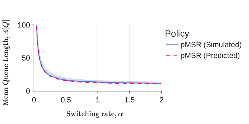
(a) pMSR

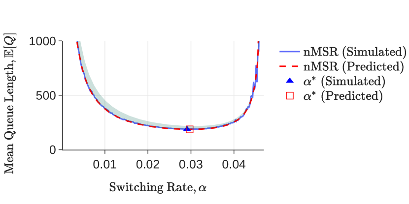
(b) nMSR

Figure 1. The effect of switching rate on MSR policies under various preemption behaviors with the example from Section 7.1. The shaded regions depict our upper and lower bounds on $\mathbb{E}[Q]$. Our pMSR policies benefit from a high switching rate when system load $\rho=0.9$. However, nMSR policies suffer when $\alpha$ is too high or too low. We see that our queue length prediction is accurate and can be used to select $\alpha^{*}$ in both cases.

In fact, we can actually prove this property using our mean queue length bounds for small pMSR instances. When all the expected relative completion terms, $\mathbb{E}[\Delta(\cdot)]$ in our upper bounds are positive, we can see that the upper bound in minimized by taking $\alpha\rightarrow\infty$. As $\alpha$ becomes large, our upper bound for type-$i$ jobs begins to look like $\frac{\rho_{i}}{1-\rho_{i}}$. This is similar to the expected number of jobs in an $M/M/1$ with load $\rho_{i}$. We prove the property in Appendix B for the case where $N^{p(\alpha)}=2$. Figure 1(a) confirms this result by showing how the mean queue length under $p(\alpha)$ improves as $\alpha$ grows. Notably, although our theoretical results show that taking $\alpha\rightarrow\infty$ is beneficial in this example, Figure 1(a) shows that we capture most of the performance benefit as long as $\alpha\geq 2$.

6.2. Choosing an nMSR Policy (Nonpreemptive MSR)

Given that we select a good pMSR policy in Section 6.1, the proof of Theorem 5 yields a related nMSR policy that stabilizes the system. Specifically, our proof suggests setting the working states to be the states of $m^{p}(t)$ and then using arbitrary switching routes between these states. To stabilize the system, we can scale the transition rates out of the working states by a very small switching rate $\alpha>0$. This method for choosing an nMSR policy has two main issues. First, switching routes are chosen arbitrarily instead of being chosen to optimize mean response time. Second, while $\alpha$ must be small to guarantee stability, the optimal switching rate $\alpha^{*}$ is not obvious here.

The space of possible switching routes between working states is generally massive. Because our queue length bounds must be derived separately for each choice of switching routes, it is hard to optimize this choice using our results. However, we sampled many possible switching routes for the nMSR example in Section 7.1 and found that the choice of switching routes had a minimal impact on mean queue length. Hence, we defer a full analysis of optimizing switching routes to future work. An example of an nMSR policy with simple switching routes is shown in Appendix D.

We do find our queue length bounds useful for optimizing the switching rates of an nMSR policy. Given a pMSR policy selected according to Section 6.1, we let $q(\alpha)$ be the nMSR policy based on $p$ whose transitions out of working states are scaled by $\alpha>0$. Unlike in the preemptive case, $q(\alpha)$ can suffer for high $\alpha$ values. In this case, the policy spends too much time in switching states, leading to higher mean queue length and possibly even instability. Conversely, if $\alpha$ is too small, the relative completions terms in our queue length bounds grow, and our mean queue length prediction also increases. We therefore use our bounds to select the optimal switching rate, $\alpha^{*}$, that balances the cost of spending time in switching states with the cost of switching too slowly between working states. Figure 1(b) shows that our mean queue length predictions allow us to accurately predict $\alpha^{*}$, and that choosing the correct value of $\alpha$ dramatically reduces mean queue length.

6.3. Choosing an sMSR Policy (MSR with Setup)

Our process for selecting an sMSR policy directly follows our selection process for an nMSR policy. The central difference between these cases is the structure of the switching routes between the policies. The switching routes of $q$ differ from the switching routes of $r$ in two key ways. First, the rates at which the policies move through the switching states will differ. While $q$ switches by waiting for completions with rate $\mu_{i}$, $r$ switches by waiting for setup times with setup rate $\gamma$. Second, the nMSR policy actually completes jobs while in its switching states, but much of the time $r$ spends in its switching states is wasted. That is, while $r$ is experiencing setup times, it is unable to complete the jobs being preempted. Nonetheless, we can use a similar process for selecting an sMSR policy based on a given pMSR policy. This includes considering a range of sMSR policies, $r(\alpha)$, whose working state transitions are scaled by $\alpha$, and using our analysis to select an optimal switching rate $\alpha^{*}$. We will compare our choices of an nMSR and sMSR policy in detail in Section 7.

7. Evaluation

We now compare our MSR policies to a several scheduling policies from the literature. We use a simple yet illustrative example of a multiresource job system (Section 7.1) to evaluate pMSR, nMSR, and sMSR policies using both our theoretical results and simulations (Section 7.2).

We compare our MSR policies against the following policies from the literature.

MaxWeight is a preemptive policy proposed in (Maguluri and Srikant, 2013) that chooses a schedule by solving a bin-packing problem on every arrival or departure. MaxWeight tries to maximize the weighted number of jobs in service, where the weight of type-$i$ jobs equals to the queue length of type-$i$ jobs.

Randomized-Timers is a non-preemptive policy proposed in (Ghaderi, 2016a) that uses moments of when jobs complete to change schedules. The policy uses a complex randomized algorithm to discover good solutions to the weighted bin-packing problem used by MaxWeight while the policy runs.

First-Fit is a simple, non-preemptive policy similar to FCFS. Sometimes known as BackFilling (Grosof et al., 2022), First-Fit examines the queued jobs in FCFS order upon each job arrival or completion. If a job is found that can be added to the set of running jobs, First-Fit serves this job. Running jobs are never preempted. First-Fit is generally thought to be a better version of the FCFS policy from Section 1.

7.1. Experimental Setup

To evaluate our MSR policies, we consider a server with three resource types (WLOG, we call the resources CPU cores, DRAM, and network bandwidth). Our example server has 20 cores, 15 GB of DRAM and 50 Gbps of network bandwidth. We assume there are three job types with demands

$${\bf D}_{1}=(3,7,1)\quad{\bf D}_{2}=(4,1,1)\quad{\bf D}_{3}=(10,1,5),$$

and that the system arrival and service rate vectors are given as

$$\bm{\lambda}=\rho\cdot(.5,2,1)\quad\bm{\mu}=(1,1,1).$$

Here, the system load, $\rho\in(0,1)$, is a constant we vary to control the load on the server. Note that $\rho<1$ implies $\bm{\lambda}\in\mathcal{C}$. This example was chosen to be non-trivial in two key ways.

First, some possible schedules in this example are Pareto optimal, but do not lie on the boundary of the convex hull of $\mathcal{S}$. For example, the schedule $(1,1,1)$ cannot fit an additional job of any type without removing some jobs from the schedule, but it does not lie on the convex boundary of $\mathcal{S}$. Hence, although the schedule $(1,1,1)$ seems to pack the server efficiently, choosing this schedule will not help stabilize the system when system load is sufficiently high.

Second, the possible schedules on the convex boundary of $\mathcal{S}$ are not trivially close together. Hence, in cases where preemption is limited, nMSR and sMSR policies will need non-trivial switching routes to move between working states. The modulating processes for the pMSR, nMSR, and sMSR policies we construct based on this example are shown in Appendix D.

7.2. Simulations

In this section, we evaluate our pMSR, nMSR, and sMSR policies on the example from Section 7.1.

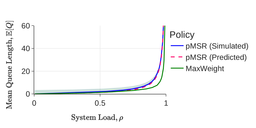
Figure 2. Mean queue length under $p(\alpha)$ compared to the preemptive MaxWeight policy. Here, we set $\alpha=2$. Our mean queue length prediction is accurate at all loads, and our pMSR policy matches the capacity region of MaxWeight. The shaded region depicts our upper and lower bounds on $\mathbb{E}[Q]$ for $p(\alpha)$.

pMSR Policies. We compare the performance of a pMSR policy to MaxWeight in Figure 2. Specifically, we construct the pMSR policy $p(\alpha)$ using the process from Section 6.1. While $p(\alpha)$ improves for large $\alpha$, our bounds suggest that setting $\alpha=2$ should suffice to obtain a low mean queue length (Figure 1(a)). Our simulations show that, despite being far simpler and more practical to implement, $p(\alpha)$ is generally competitive with MaxWeight. While MaxWeight outperforms $p(\alpha)$ at higher loads, both policies are stable as $\rho$ approaches 1. We note that our mean queue length predictions are highly accurate at all loads in this example.

nMSR Policies.

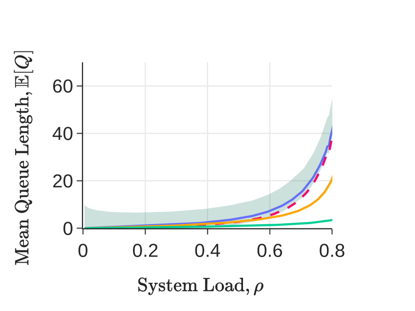
(a) nMSR at low loads

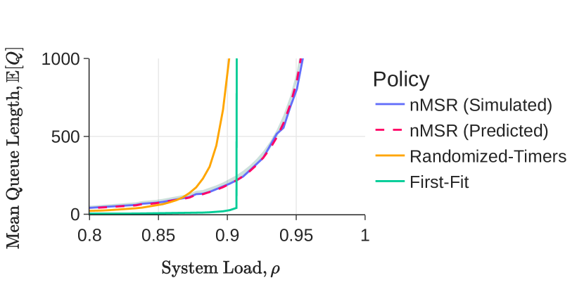
(b) nMSR at high loads

Figure 3. Performance evaluation of the nMSR policy, $q(\alpha^{*})$, on the example from Section 7.1. We consider lower loads $(\rho<.8)$ in (a) and higher loads $(\rho>.8)$ in (b). For each value of $\rho$ we compute the optimal switching rate, $\alpha^{*}$. We compare $q(\alpha^{*})$ to other non-preemptive policies from the literature. While $q(\alpha^{*})$ is not the best policy at intermediate loads, it greatly outperforms the competitor policies when load is high ($\rho>.9$). The shaded regions depict our upper and lower bounds on $\mathbb{E}[Q]$ for our nMSR policy.

To evaluate nMSR policies, we compare $q(\alpha^{*})$ as chosen in Section 6.2 to the non-preemptive Randomized-Timers and First-Fit policies. Figure 3 shows that, although our nMSR policy is not always the best, it is the best of the non-preemptive policies system load is high. Here, First-Fit becomes unstable because it repeatedly chooses to use the schedule $(1,1,1)$. Randomized-Timers also performs poorly under high load because it changes between schedules too slowly when queue lengths are long. In fact, Randomized-Timers performed so poorly under high load that many of our simulations did not converge (these points were omitted). The nMSR policy does struggle at intermediate loads, where $q(\alpha^{*})$ would benefit from fast switching between working states. Here, $q(\alpha^{*})$ is held back by its relatively slow non-preemptive switching routes.

sMSR Policies. To our knowledge, no multiresource job scheduling policies from the literature are designed to account for jobs with setup times. However, when scheduling jobs with setup times, it is always possible to use an nMSR policy and avoid costly preemptions altogether. Hence, it is natural to compare the sMSR policy from Section 6.3, $r(\alpha^{*})$, to the nMSR policy $q(\alpha^{*})$. One might also ask how fast the setup times must be in order for $r(\alpha^{*})$ to approximate the performance of the pMSR policy $p(\alpha)$ with high $\alpha$. We address both of these questions using our mean queue length bounds.

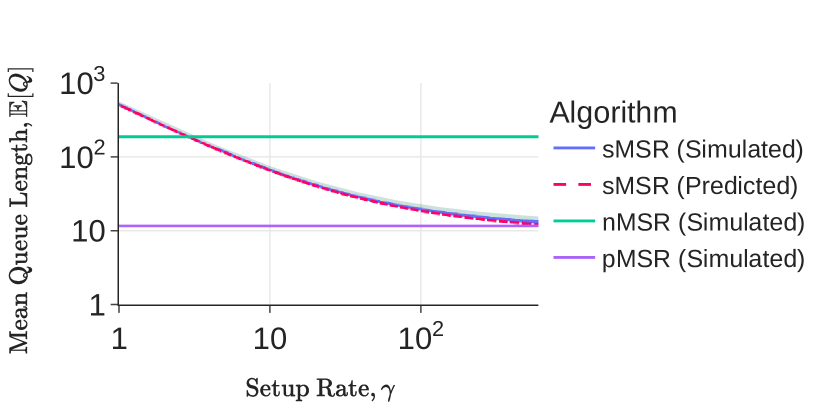
Figure 4. Mean queue length of the sMSR policy $r(\alpha^{*})$ as a function of the setup rate, $\gamma$. Here, system load $\rho=0.9$. The shaded regions depict our upper and lower bounds on $\mathbb{E}[Q]$ for $r(\alpha^{*})$. We compare the performance of $r(\alpha^{*})$ to the nMSR policy $q(\alpha^{*})$ and the pMSR policy $p(\alpha^{*})$ with fully preemptible jobs.

Intuitively, $r(\alpha^{*})$ should perform better than $q(\alpha^{*})$ when $\gamma$ is significantly higher than $\mu_{i}$ for all $i$. In this case, the sMSR policy will tolerate some setup times in order to switch between working states more quickly than the nMSR policy. However, this comparison is non-trivial because an nMSR policy continues to complete jobs while in switching states, whereas the sMSR policy cannot complete jobs that are being preempted. Similarly, when $\gamma$ is quite high, we should see the performance of $r(\alpha^{*})$ approach the performance of $p(\alpha)$. When $\gamma$ is very low, on the other hand, $r(\alpha^{*})$ suffers due to long setup times. It is not immediately clear how our sMSR policy compares to our pMSR and nMSR policies as a function of $\gamma$.

Figure 4 shows that our mean queue length bounds accurately predict the sensitivity of $r(\alpha^{*})$ to changes in $\gamma$. Additionally, we see that average setup times must be significantly shorter (3x shorter) than an average service time for the sMSR policy to outperform the nMSR policy. Additionally, we see that setup times must be roughly 100x shorter than a service time on average in order to achieve performance close to that of a fully preemptive pMSR policy. Our mean queue length prediction accurately predicts the performance of $r(\alpha^{*})$ for all values of $\gamma$. In these experiments, we used our mean queue length bounds to select a different $\alpha^{*}$ for each policy and for each value of $\gamma$.

8. Conclusion

This paper considers scheduling a stream of multiresource jobs. We devise a class of low-complexity scheduling policies, called MSR policies. An MSR policy selects a set of candidate schedules and switches between these schedules according to a CTMC. The class of MSR policies is throughput-optimal despite its simplicity. By analyzing the stability and mean queue length of MSR policies, we show how to select an MSR policy that achieves low mean response time in a variety of practical cases. Specifically, we analyze the case of scheduling preemptible jobs, non-preemptible jobs, and the case where preemptions incur a setup time.

While our current method of analyzing MSR policies yields accurate predictions of mean queue lengths, the class of MSR policies has some limitations. Specifically, our pMSR policies are outperformed by the MaxWeight policy at moderate loads, and our nMSR policies are outperformed by First-Fit at moderate loads. Both of these competitor policies have modulating processes with an infinite number of states and with transitions that depend heavily on the state of the system. Our current analytic techniques do not apply to policies with these complex modulating processes. Hence, a natural direction for future work is to begin to bridge this divide by designing policies that incorporate some state-dependent behavior, like MaxWeight and First-Fit, while remaining analytically tractable. By generalizing our analysis of Markov-modulated service rate systems, we hope to analyze scheduling policies that achieve low mean response time at all system loads.

Appendix

Appendix A Proof of Theorem 2

Theorem 0.

For any job type, $i$, consider an MSR policy $p$ and its corresponding MSR-1 policy $p\mbox{-}1$. Let $\beta_{i}^{p}$ denote the maximum number of type-$i$ jobs served in parallel $p$. Then,

$$\mathbb{E}[Q_{i}^{p\mbox{-}1}]\leq\mathbb{E}[Q^{p}_{i}]\leq\mathbb{E}[Q_{i}^{p\mbox{-}1}]+\beta_{i}^{p}.$$

Proof.

We prove this claim via a coupling argument. First, observe that the arrival processes and modulating processes are identical between the MSR and MSR-1 systems. Hence, to compare the two systems on a given sample path, we will assume that arrival times are the same in both systems and that both systems’ modulating processes are in corresponding states at any time $t$.

Next, we couple the departure processes of the two systems as follows. At any time, $t$, the MSR system attempts to serve ${\bf u}^{p}_{i}(t)$ type-$i$ jobs in parallel. Similarly, the service rate of type-$i$ jobs in the MSR-1 system is $\mu_{i}{\bf u}^{p}_{i}(t)$. To couple the systems, we set ${\bf u}^{p}_{i}(t)$ exponential timers at any time $t$ corresponding to an event (arrival, departure, or change to the modulating process) in either system. If one of these timers expires before the next event, it triggers a type-$i$ completion in the MSR-1 system as long as there is at least one job to complete. In the MSR system, we map the type-$i$ jobs in service at time $t$ to one timer each. Note that this means some timers may not have an associated job. If a timer expires that is associated with a job in the MSR system, this associated job completes.

We will show that, for any sample path under our coupling,

(11) $$Q_{i}^{p\mbox{-}1}(t)\leq Q^{p}_{i}(t)\leq Q_{i}^{p\mbox{-}1}(t)+\beta_{i}^{p}\quad\forall t\geq 0$$

We prove this claim by induction on $t$. Without loss of generality, we assume that the claim holds at time 0 where $Q_{i}^{p\mbox{-}1}(0)=Q^{p}_{i}(0)=0$. Consider any time $t$ where (11) is assumed to hold for induction. We will consider two cases.

First, consider the case where $Q_{i}^{p}(t)<\beta_{i}^{p}$. Let $t^{\prime}$ be the next time after time $t$ where $Q_{i}^{p}(t)=\beta_{i}^{p}$. In the interval $[t,t^{\prime}]$, any completion in the MSR system corresponds to a completion in the MSR-1 system, unless the MSR-1 system has 0 type-$i$ jobs. Hence, $Q_{i}^{p\mbox{-}1}(t)\leq Q^{p}_{i}(t)$ implies that at each successive completion time $c\in[t,t^{\prime}]$, $Q_{i}^{p\mbox{-}1}(c)\leq Q^{p}_{i}(c)$. Because arrivals affect both systems equally, we have that $Q_{i}^{p\mbox{-}1}(\tau)\leq Q^{p}_{i}(\tau)$ for each arrival time $\tau\in[t,t^{\prime}]$. Finally, because $Q_{i}^{p}(\tau)\leq\beta_{i}^{p}$ for $\tau\in[t,t^{\prime}]$, it is trivial to see that $Q_{i}^{p}(\tau)\leq Q_{i}^{p\mbox{-}1}(\tau)+\beta_{i}^{p}$ for $\tau\in[t,t^{\prime}]$.

Second, consider the case where $Q_{i}^{p}(t)\geq\beta_{i}^{p}$. Let $t^{\prime}$ be the next time after $t$ where $Q_{i}^{p}(t)<\beta_{i}^{p}$. In the interval $[t,t^{\prime}]$, any completion in the MSR system corresponds to a completion in the MSR-1 system, unless the MSR-1 system has 0 type-$i$ jobs. This once again implies that the first part of the inequality holds on the interval $[t,t^{\prime}]$. To prove the second part of the inequality, note that now any completion in the MSR-1 system necessarily corresponds to a completion in the MSR system, since the MSR system has a job associated with every timer for the entire interval. Hence, $Q_{i}^{p}(t)\leq Q^{p\mbox{-}1}_{i}(t)+\beta_{i}^{p}$ implies that at each successive completion time $c\in[t,t^{\prime}]$, $Q_{i}^{p}(c)\leq Q^{p\mbox{-}1}_{i}(c)+\beta_{i}^{p}$ because every decrease in $Q^{p\mbox{-}1}_{i}$ corresponds to a simultaneous decrease in $Q^{p}_{i}$. Thus, $Q_{i}^{p}(\tau)\leq Q_{i}^{p\mbox{-}1}(\tau)+\beta_{i}^{p}$ for $\tau\in[t,t^{\prime}]$.

Hence, given that (11) holds at time $t$, it also holds on the entire interval $[t,t^{\prime}]$, where $t^{\prime}$ is at least one event time later than $t$. This completes the proof of (11) by induction.

Given that $\eqref{eq:induct}$ holds for any sample path under our coupling, we have

$$Q_{i}^{p\mbox{-}1}\leq_{st}Q^{p}_{i}\leq_{st}Q_{i}^{p\mbox{-}1}+\beta_{i}^{p}$$

and thus

$$\mathbb{E}[Q_{i}^{p\mbox{-}1}]\leq\mathbb{E}[Q^{p}_{i}]\leq\mathbb{E}[Q_{i}^{p\mbox{-}1}]+\beta_{i}^{p}$$

as desired. ∎

Appendix B Switching Rates for Preemptive MSR Policies

Theorem 1.

For a two-state pMSR policy $p$, where $N^{p}=2$, the mean queue length upper bound is minimized if we are switching schedules infinitely often. That is, $\alpha=\infty$ minimizes the mean length upper bound across all $p(\alpha)$’s.

Proof.

Let $\alpha{\bf G}^{p}=\begin{pmatrix}-\alpha x_{1}&\alpha x_{1}\\ \alpha x_{2}&-\alpha x_{2}\end{pmatrix}$ for some $x_{1},x_{2}>0$. WLOG, we assume $u_{1,1}^{p\mbox{-}1}\geq u_{2,1}^{p\mbox{-}1}$. Let $w_{1},w_{2}$ be two working states and of system. By Lemma 5, we get

$$\begin{cases}\begin{pmatrix}-\alpha x_{1}&\alpha x_{1}\\ \alpha x_{2}&-\alpha x_{2}\end{pmatrix}(\Delta_{1}(1),\Delta_{1}(2))=\mathbb{E}[u_{1}^{p\mbox{-}1}](1,1)-(u_{1,1}^{p\mbox{-}1},u_{2,1}^{p\mbox{-}1})\\ \Delta_{1}(1){\bf P}\{u_{1}^{p\mbox{-}1}=w_{1}\}+\Delta_{1}(2){\bf P}\{u_{1}^{p\mbox{-}1}=w_{2}\}=0\end{cases}$$

Also, by the definition of CTMC, we have

$$\begin{cases}\begin{pmatrix}-\alpha x_{1}&\alpha x_{1}\\ \alpha x_{2}&-\alpha x_{2}\end{pmatrix}\begin{pmatrix}{\bf P}\{u_{1}^{p\mbox{-}1}=w_{1}\}&{\bf P}\{u_{1}^{p\mbox{-}1}=w_{2}\}\end{pmatrix}=0\end{cases}.$$

Hence,

$$\begin{cases}{\bf P}\{u_{1}^{p\mbox{-}1}=w_{1}\}=\frac{x_{2}}{x_{1}+x_{2}}\\ {\bf P}\{u_{1}^{p\mbox{-}1}=w_{2}\}=\frac{x_{1}}{x_{1}+x_{2}}\end{cases}.$$

By definition of $v_{1}$, we have

$$\begin{cases}{\bf P}\{v_{1}^{p\mbox{-}1}=w_{1}\}=\frac{u_{1,1}^{p\mbox{-}1}}{\mathbb{E}[u_{1}^{p\mbox{-}1}]}\frac{x_{2}}{x_{1}+x_{2}}\\ {\bf P}\{v_{1}^{p\mbox{-}1}=w_{2}\}=\frac{u_{2,1}^{p\mbox{-}1}}{\mathbb{E}[u_{1}^{p\mbox{-}1}]}\frac{x_{1}}{x_{1}+x_{2}}\end{cases}.$$

Solving this system, we get

$$\begin{cases}\Delta_{1}(1)=\alpha x_{1}\frac{u_{1,1}^{p\mbox{-}1}-u_{2,1}^{p\mbox{-}1}}{(x_{1}+x_{2})^{2}}\\ \Delta_{1}(2)=\alpha x_{2}\frac{u_{2,1}^{p\mbox{-}1}-u_{1,1}^{p\mbox{-}1}}{(x_{1}+x_{2})^{2}}\end{cases}.$$

Plugging into Theorem 4, we get

$$\mathbb{E}[Q_{1}^{p(\alpha)}]=\frac{\rho_{1}}{1-\rho_{1}}+\frac{x_{1}x_{2}(u_{1,1}^{p\mbox{-}1}-u_{2,1}^{p\mbox{-}1})^{2}}{\alpha\mathbb{E}[u_{1}^{p\mbox{-}1}](1-\rho_{1})(x_{1}+x_{2})^{3}}+B,$$

where $x_{2}\frac{u_{2,1}^{p\mbox{-}1}-u_{1,1}^{p\mbox{-}1}}{\alpha(x_{1}+x_{2})^{2}}\leq B\leq x_{1}\frac{u_{1,1}^{p\mbox{-}1}-u_{2,1}^{p\mbox{-}1}}{\alpha(x_{1}+x_{2})^{2}}$. Thus,

$$\mathbb{E}[Q_{1}^{p(\alpha)}]\leq\frac{\rho_{1}}{1-\rho_{1}}+\frac{x_{1}x_{2}(u_{1,1}^{p\mbox{-}1}-u_{2,1}^{p\mbox{-}1})^{2}}{\alpha\mathbb{E}[u_{1}^{p\mbox{-}1}](1-\rho_{1})(x_{1}+x_{2})^{3}}+x_{1}\frac{u_{1,1}^{p\mbox{-}1}-u_{2,1}^{p\mbox{-}1}}{\alpha(x_{1}+x_{2})^{2}}.$$

Let $z=\frac{x_{1}x_{2}(u_{1,1}^{p\mbox{-}1}-u_{2,1}^{p\mbox{-}1})^{2}}{\alpha\mathbb{E}[u_{1}^{p\mbox{-}1}](1-\rho_{1})(x_{1}+x_{2})^{3}}+x_{1}\frac{u_{1,1}^{p\mbox{-}1}-u_{2,1}^{p\mbox{-}1}}{\alpha(x_{1}+x_{2})^{2}}$. We can see that $\lim_{\alpha\rightarrow\infty}z=0$ and that $z\geq 0$. Analysis on $\mathbb{E}[Q_{2}^{p}]$ upper bound is analogous.

Hence, we have shown that setting $\alpha=\infty$ minimizes this queue length upper bound. ∎

Appendix C Proof of Theorem 5

Theorem 0.

When scheduling non-preemptible jobs, the class of nMSR policies is throughput-optimal. That is, if there exists a scheduling policy that can stabilize a multiresource job system with $K$ job types and arrival rates $\bm{\lambda}$, then there exists an nMSR policy, $q$, with $N^{q}=K$ working states that stabilizes the system. Specifically, an nMSR policy can stabilize a system with preemptible jobs when $\bm{\lambda}\in\mathcal{C}$.

Proof.

From Theorem 4, we know that there exists an MSR policy $p$ that can stabilize the system. Hence, given some MSR policy $p$ that stabilizes the system, we will show how to construct a non-preemptive policy that also stabilizes the system.

Obviously, if $p$ is already non-preemptive, we have proven our claim. Otherwise, we can use $p$ to construct an nMSR policy that stabilizes the system.

To do this, we first define $p(\alpha)$ to be the MSR policy that with infinitesimal generator ${\bf G}^{p(\alpha)}=\alpha{\bf G}^{p}$. That is, $p(\alpha)$ is an MSR policy whose modulating process is a scaled version of $p$’s modulating process. We will create a non-preemptive policy, $q(\alpha)$, that is based on $p(\alpha)$. To make $q(\alpha)$ non-preemptive, we must add some switching states between the states of $p(\alpha)$’s modulating process. The original states of $p(\alpha)$’s modulating process will form the working states of $q(\alpha)$. We assume that the added switching states form arbitrary (finite length) switching routes between these working states. Hence, $q(\alpha)$ is a valid nMSR policy. We will now show that, for sufficiently small $\alpha$, $q(\alpha)$ stabilizes the system.

Let $w_{1},w_{2},\cdots,w_{N^{p}}$ denote the working states of $q(\alpha)$, and let $s_{1},s_{2},\cdots,s_{N^{q}-N^{p}}$ denote all the switching states of $q(\alpha)$. Let $\pi^{q(\alpha)}$ denote the stationary distribution of states in the modulating process of $q(\alpha)$. Let $\pi_{W}^{q(\alpha)}$ be the probability that we are in any working state defined as

$$\pi_{W}^{q(\alpha)}=\sum_{i=1}^{N^{p}}\pi_{w_{i}}^{q(\alpha)}.$$

By Lemma 2, we have $\bm{\mu}\otimes\mathbb{E}[{\bf u}^{p}]>\bm{\lambda}$. Therefore, there exists $\epsilon_{1}>0$ such that $\bm{\mu}\otimes\mathbb{E}[{\bf u}^{p}]-\epsilon_{1}=\bm{\lambda}$. Next, we condition $\mathbb{E}[{\bf u}^{q(\alpha)}]$ on whether it is in working state.

$$\mathbb{E}[{\bf u}^{q(\alpha)}] =\mathbb{E}[{\bf u}^{q(\alpha)}\mid\text{working state}]\pi_{W}^{q(\alpha)}+\mathbb{E}[{\bf u}^{q(\alpha)}\mid\text{not working state}](1-\pi_{W}^{q(\alpha)})$$

$$\geq\mathbb{E}[{\bf u}^{q(\alpha)}\mid\text{working state}]\pi_{W}^{q(\alpha)}$$

$$=\mathbb{E}[{\bf u}^{p(\alpha)}]\pi_{W}^{q(\alpha)}$$

$$=\mathbb{E}[{\bf u}^{p}]\pi_{W}^{q(\alpha)}$$

Because Lemma 2 tells us that $\mathbb{E}[{\bf u}^{p}]-\epsilon_{1}=\bm{\lambda}$ for some $\epsilon_{1}>0$, it will suffice to show that $\pi_{W}^{q(\alpha)}$ can be arbitrarily close to 1 when $\alpha$ is small. We prove this in the Lemma 1.

Lemma 1.

For any $\epsilon>0$, there exists an $\alpha$ such that

$$\pi_{W}^{q(\alpha)}>1-\epsilon$$

Proof.

We will prove the Lemma via the renewal-reward theorem(Harchol-Balter, 2013). We let the renewal cycle be the time between visits to state $w_{1}$ by ${\bf u}^{q(\alpha)}(t)$. Consider a path ${\bf u}^{q(\alpha)}(t)$ takes, $\omega$, during a renewal cycle, we use the random variable $X$ to define the cycle length and let the reward function be $R^{q(\alpha)}(t)=\bm{1}[{\bf u}^{q(\alpha)}(t)\text{ is in a working state}]$. Let $R^{q(\alpha)}$ be the random variable denoting the reward accrued during one renewal cycle. Let $S^{q(\alpha)}$ be the random variable denoting the time ${\bf u}^{q(\alpha)}$ spends in switching states during a renewal cycle.

Then, by the renewal-reward theorem (Harchol-Balter, 2013), we have

$$\pi_{W}^{q(\alpha)} =\frac{\mathbb{E}[R^{q(\alpha)}]}{\mathbb{E}[X]}$$

$$=\frac{\mathbb{E}[R^{q(\alpha)}]}{\mathbb{E}[R^{q(\alpha)}]+\mathbb{E}[S^{q(\alpha)}]}$$

(12) $$=\frac{\frac{1}{\alpha}\mathbb{E}[R^{q(1)}]}{\frac{1}{\alpha}\mathbb{E}[R^{q(1)}]+\mathbb{E}[S^{q(1)}]}$$

$$=\frac{\mathbb{E}[R^{q(1)}]}{\mathbb{E}[R^{q(1)}]+\alpha\mathbb{E}[S^{q(1)}]}.$$

Step (12) follows from

$$\mathbb{E}[R^{q(\alpha)}] =\sum_{\omega}\mathbb{E}[R^{q(\alpha)}\mid\omega]{\bf P}\{\omega\}$$

$$=\sum_{\omega}\frac{1}{\alpha}\mathbb{E}[R^{q(1)}\mid\omega]{\bf P}\{\omega\}$$

$$=\frac{1}{\alpha}\mathbb{E}[R^{q(1)}]$$

because the transition rates out of the working states are being multiplied by $\alpha$ in $q(\alpha)$ compared to $q(1)$. Therefore, we only need to set the $\alpha$ to be

$$0<\alpha<\frac{\epsilon\mathbb{E}[R^{q(1)}]}{(1-\epsilon)\mathbb{E}[S^{q(1)}]}$$

such that $\pi_{W}^{q(\alpha)}>1-\epsilon$. ∎

From Lemma 1, we know that there exists some $\alpha$ such that $\pi_{W}^{q(\alpha)}=1-\epsilon_{2}$ holds for a given $\epsilon_{2}>0$. Hence, if we are scaling the transitions out of working states by $\alpha$, we have,

$$\bm{\mu}\otimes\mathbb{E}[{\bf u}^{q}] =\bm{\mu}\otimes\mathbb{E}[{\bf u}^{p}]\pi_{W}(\alpha)$$

$$>\bm{\mu}\otimes\mathbb{E}[{\bf u}^{p}](1-\epsilon_{2})$$

$$=(\bm{\lambda}+\epsilon_{1})(1-\epsilon_{2})$$

$$=\bm{\lambda}+\epsilon_{1}-\epsilon_{2}-\epsilon_{1}\epsilon_{2}.$$

In this case, we can set $\epsilon_{3}=\epsilon_{1}-\epsilon_{2}-\epsilon_{1}\epsilon_{2}$. We need $\epsilon_{3}=\epsilon_{1}(1-\epsilon_{2})-\epsilon_{2}>0$. Therefore, given $\epsilon_{1}$, we can set $\epsilon_{2}$ to be $\frac{\epsilon_{2}}{1-\epsilon_{2}}<\epsilon_{1}$.

Lastly, by invoking Lemma 2, we have shown that the constructed nMSR policy with the $\alpha$ associated with $\epsilon_{2}$ can stabilize the system. ∎

Appendix D Modulating Processes

(a) The modulating process of the pMSR policy, $p(\alpha)$

(b) The modulating process of the nMSR policy, $q(\alpha)$

(c) The modulating process of the sMSR policy, $r(\alpha)$

Figure 5. Here we depict the structure of the modulating processes for $p(\alpha)$, $q(\alpha)$ and $r(\alpha)$. These policies are used for the examples described in Section 7.1. States marked with $w$ are working states, and states marked with $t$ are switching states. In (a) and (b), the subscripts denote the state’s corresponding schedule. In (c), the subscripts for switching states denote the number of jobs experiencing a setup time due to being preempted.

References

- (1)
- Burman and Smith (1986) David Y Burman and Donald R Smith. 1986. An asymptotic analysis of a queueing system with Markov-modulated arrivals. Operations Research 34, 1 (1986), 105–119.
- Ciucu and Poloczek (2018) Florin Ciucu and Felix Poloczek. 2018. Two extensions of Kingman’s GI/G/1 bound. Proceedings of the ACM on Measurement and Analysis of Computing Systems 2, 3 (2018), 1–33.
- Delimitrou and Kozyrakis (2014) Christina Delimitrou and Christos Kozyrakis. 2014. Quasar: Resource-efficient and qos-aware cluster management. ACM SIGPLAN Notices 49, 4 (2014), 127–144.
- Dimitrov (2011) Mitko Dimitrov. 2011. Single-server queueing system with Markov-modulated arrivals and service times. Pliska Stud. Math. Bulg 20 (2011), 53–62.
- Eryilmaz and Srikant (2012) Atilla Eryilmaz and Rayadurgam Srikant. 2012. Asymptotically tight steady-state queue length bounds implied by drift conditions. Queueing Systems 72 (2012), 311–359.
- Fabila-Monroy and Huemer (2017) Ruy Fabila-Monroy and Clemens Huemer. 2017. Caratheodory’s theorem in depth. Discrete & Computational Geometry 58 (2017), 51–66.
- Falin and Falin (1999) Gennadi Falin and Anatoli Falin. 1999. Heavy traffic analysis of M/G/1 type queueing systems with Markov-modulated arrivals. Top 7, 2 (1999), 279–291.
- Gandhi et al. (2013) Anshul Gandhi, Sherwin Doroudi, Mor Harchol-Balter, and Alan Scheller-Wolf. 2013. Exact analysis of the M/M/k/setup class of Markov chains via recursive renewal reward. In Proceedings of the ACM SIGMETRICS/international conference on Measurement and modeling of computer systems. 153–166.
- Ghaderi (2016a) Javad Ghaderi. 2016a. Randomized algorithms for scheduling VMs in the cloud. Proceedings - IEEE INFOCOM 2016-July (7 2016). https://doi.org/10.1109/INFOCOM.2016.7524536
- Ghaderi (2016b) Javad Ghaderi. 2016b. Simple high-performance algorithms for scheduling jobs in the cloud. 2015 53rd Annual Allerton Conference on Communication, Control, and Computing, Allerton 2015 (4 2016), 345–352. https://doi.org/10.1109/ALLERTON.2015.7447025
- Grosof et al. (2020) Isaac Grosof, Mor Harchol-Balter, and Alan Scheller-Wolf. 2020. Stability for Two-class Multiserver-job Systems. (10 2020). https://arxiv.org/abs/2010.00631v1
- Grosof et al. (2022) Isaac Grosof, Mor Harchol-Balter, and Alan Scheller-Wolf. 2022. WCFS: a new framework for analyzing multiserver systems. Queueing Systems 102, 1-2 (10 2022), 143–174. https://doi.org/10.1007/S11134-022-09848-6/METRICS
- Grosof et al. (2024) Isaac Grosof, Yige Hong, and Mor Harchol-Balter. 2024. Analysis of Markovian Arrivals and Service with Applications to Intermittent Overload. arXiv preprint arXiv:2405.04102 (2024).
- Grosof et al. (2023) Isaac Grosof, Yige Hong, Mor Harchol-Balter, and Alan Scheller-Wolf. 2023. The RESET and MARC techniques, with application to multiserver-job analysis. Performance Evaluation 162 (2023), 102378.
- Harchol-Balter (2013) M. Harchol-Balter. 2013. Performance Modeling and Design of Computer Systems: Queueing Theory in Action. Cambridge University Press.
- Harchol-Balter (2022) Mor Harchol-Balter. 2022. The multiserver job queueing model. Queueing Systems 100, 3 (2022), 201–203.
- Hindman et al. (2011) Benjamin Hindman, Andy Konwinski, Matei Zaharia, Ali Ghodsi, Anthony D Joseph, Randy H Katz, Scott Shenker, and Ion Stoica. 2011. Mesos: A platform for fine-grained resource sharing in the data center.. In NSDI, Vol. 11. 22–22.
- Im et al. (2015) Sungjin Im, Nathaniel Kell, Janardhan Kulkarni, and Debmalya Panigrahi. 2015. Tight Bounds for Online Vector Scheduling. Proceedings - Annual IEEE Symposium on Foundations of Computer Science, FOCS 2015-December (12 2015), 525–544. https://doi.org/10.1109/FOCS.2015.39
- Lipari (2012) Don Lipari. 2012. The SLURM Scheduler Design. SLURM User Group. http://slurm. schedmd. com/slurm_ug_2012/SUG-2012-Scheduling. pdf (2012).
- Maguluri and Srikant (2013) Siva Theja Maguluri and Rayadurgam Srikant. 2013. Scheduling jobs with unknown duration in clouds. IEEE/ACM Transactions On Networking 22, 6 (2013), 1938–1951.
- Maguluri et al. (2014) Siva Theja Maguluri, R. Srikant, and Lei Ying. 2014. Heavy traffic optimal resource allocation algorithms for cloud computing clusters. Performance Evaluation 81 (2014), 20–39. https://doi.org/10.1016/j.peva.2014.08.002
- Neuts (1978) Marcel F Neuts. 1978. The M/M/1 queue with randomly varying arrival and service rates. Opsearch 15 (1978), 139–157.
- Psychas and Ghaderi (2018) Konstantinos Psychas and Javad Ghaderi. 2018. Randomized algorithms for scheduling multi-resource jobs in the cloud. IEEE/ACM Transactions on Networking 26, 5 (10 2018), 2202–2215. https://doi.org/10.1109/TNET.2018.2863647
- Regterschot and De Smit (1986) GJK Regterschot and JHA De Smit. 1986. The queue M//G/1 with Markov modulated arrivals and services. Mathematics of operations research 11, 3 (1986), 465–483.
- SchedMD (2021) SchedMD. 2021. SLURM Workload Manager. (2021). https://slurm.schedmd.com/heterogeneous_jobs.html.
- Stolyar (2004) Alexander L. Stolyar. 2004. MaxWeight scheduling in a generalized switch: State space collapse and workload minimization in heavy traffic. https://doi.org/10.1214/aoap/1075828046 14, 1 (2 2004), 1–53. https://doi.org/10.1214/AOAP/1075828046
- Tirmazi et al. (2020) Muhammad Tirmazi, Adam Barker, Nan Deng Google, Md E Haque Google, Zhijing Gene Qin Google, Steven Hand Google, Mor Harchol-Balter CMU, John Wilkes Google, Nan Deng, Md E Haque, Zhi-jing Gene Qin, Steven Hand, Mor Harchol-Balter, and John Wilkes. 2020. Borg: The next generation. Proceedings of the 15th European Conference on Computer Systems, EuroSys 2020 (4 2020), 14. https://doi.org/10.1145/3342195.3387517
- Verma et al. (2015) Abhishek Verma, Luis Pedrosa, Madhukar Korupolu, David Oppenheimer, Eric Tune, and John Wilkes. 2015. Large-scale cluster management at Google with Borg. In Proceedings of the Tenth European Conference on Computer Systems (Bordeaux, France) (EuroSys ’15). Association for Computing Machinery, New York, NY, USA, Article 18, 17 pages. https://doi.org/10.1145/2741948.2741964
- Weina Wang and Harchol-Balter (2021) Qiaomin Xie Weina Wang and Mor Harchol-Balter. 2021. Zero Queueing for Multi-Server Jobs. Proceedings of the ACM on Measurement and Analysis of Computing Systems 5, 1 (2 2021), 1–25. https://doi.org/10.1145/3447385