Goal-Conditioned Supervised Learning for Multi-Objective Recommendation

Abstract

Multi-objective learning endeavors to concurrently optimize multiple objectives using a single model, aiming to achieve high and balanced performance across these diverse objectives. However, it often involves a more complex optimization problem, particularly when navigating potential conflicts between objectives, leading to solutions with higher memory requirements and computational complexity. This paper introduces a Multi-Objective Goal-Conditioned Supervised Learning (MOGCSL) framework for automatically learning to achieve multiple objectives from offline sequential data. MOGCSL extends the conventional Goal-Conditioned Supervised Learning (GCSL) method to multi-objective scenarios by redefining goals from one-dimensional scalars to multi-dimensional vectors. The need for complex architectures and optimization constraints can be naturally eliminated. MOGCSL benefits from filtering out uninformative or noisy instances that do not achieve desirable long-term rewards. It also incorporates a novel goal-choosing algorithm to model and select “high” achievable goals for inference.

While MOGCSL is quite general, we focus on its application to the next action prediction problem in commercial-grade recommender systems. In this context, any viable solution needs to be reasonably scalable and also be robust to large amounts of noisy data that is characteristic of this application space. We show that MOGCSL performs admirably on both counts. Specifically, extensive experiments conducted on real-world recommendation datasets validate its efficacy and efficiency. Also, analysis and experiments are included to explain its strength in discounting the noisier portions of training data in recommender systems.

1 Introduction

Multi-objective learning techniques typically aim to train a single model to determine a policy for multiple objectives, which are often defined on different types of tasks (Ruder 2017; Sener and Koltun 2018; Zhang and Yang 2021). For instance, two common tasks in recommender systems are to recommend items that users may click or purchase, and hence the corresponding two objectives are defined as pursuing higher click rate and higher purchase rate. However, learning for multiple objectives simultaneously is often nontrivial, particularly when there are potential inherent conflicts among these objectives (Sener and Koltun 2018).

Existing approaches to multi-objective learning broadly address this optimization issue by formulating and optimizing a loss function that takes into account multiple objectives in a supervised learning paradigm. Some previous research focused on designing model architectures specifically for multi-objective scenarios, including the shared-bottom structure (Ma et al. 2018), the experts and task gating networks (Ma et al. 2018), and so on. Another line of research studies how to constrain the optimization process based on various assumptions regarding how to assign reasonable loss weights (Liu, Johns, and Davison 2019) or adjust gradients dynamically (Yu et al. 2020). Lin et al. (2020) proposes an optimization algorithm within the context of Pareto efficiency. We remark that these approaches often introduce substantial space and computational complexity (Ma et al. 2018; Zhang and Yang 2021). Also, they treat all the data uniformly (m-estimation). In recommender systems, sometimes none of the items shown to a user are of interest, rendering their choice uninformative. Also users are often distracted or their interests temporarily change. These are some of the reasons that the observed interaction data in real settings suffer from substantial uninformative or ”noisy” components that are better left discounted. Existing approaches do not cater well to this aspect of our focus application.

To address these issues, we propose a novel method called Multi-Objective Goal-Conditioned Supervised Learning (MOGCSL). In this framework, we first apply goal-conditioned supervised learning (GCSL) (Yang et al. 2022; Liu, Zhu, and Zhang 2022) to the multi-objective recommendation problem by introducing a new multi-dimensional goal. At its core, GCSL aims to primarily learn from the behaviors of those sessions where the long-term reward ends up being high, thereby discounting noisy user choices coming with low long-term rewards. Unlike conventional GCSL, however, we represent the reward gained from the environment with a vector instead of a scalar. Each dimension of this vector indicates the reward for a certain objective. The “goal” in MOGCSL can then be defined as a vector of desirable cumulative rewards on all of the objectives given the current state. By incorporating these goals as input, MOGCSL learns to rely only on high-fidelity portions of the data with less noise, which helps to better predict users’ real preference. Extensive experiments on two public datasets indicate that MOGCSL significantly outperforms other baselines and benefits from lower complexity.

For inference of GCSL, most previous works employ a simple goal-choosing strategy (Chen et al. 2021; Xin et al. 2023) (e.g., some multiple of the average goal in training). Although we observe that simple choices for MOGCSL do reasonably well in practice, we also introduce a novel goal-choosing algorithm that estimates the distribution of achievable goals using variational auto-encoders, and automates the selection of desirable “high” goals as input for inference. By comparing the proposed method with simpler statistical strategies, we gain valuable insights into the goal-choosing process and trade-offs for practical implementation.

Our key contributions can be summarized as follows:

• We introduce a general supervised framework called MOGCSL for multi-objective recommendations that, by design, selectively leverages training data with desirable long-term rewards. We implement this approach using a transformer encoder optimized with a standard cross-entropy loss, avoiding more complex architectures or optimization constraints that are typical for multi-objective learning. Empirical experiments on real-world e-commerce datasets demonstrate the superior efficacy and efficiency of MOGCSL.

• We comprehensively analyze the working mechanism of MOGCSL, revealing its capability to remove harmful effects of potentially noisy instances in the training data.

• As a part of MOGCSL, we introduce a goal-choosing algorithm that can model the distribution of achievable goals over interaction sequences and choose desirable ”high” goals for inference.

2 Related Works

Multi-Objective Learning. Multi-objective learning typically investigates the construction and optimization of models that can simultaneously achieve multiple objectives. Existing research primarily focuses on resolving the problem by model architecture designs (Ma et al. 2018; Misra et al. 2016) and optimization constraints (Liu, Johns, and Davison 2019; Yu et al. 2020; Lin et al. 2020). All of these works give equal weight to all instances in the training data, instead of forcefully distinguishing noisy data from non-noisy data by considering their different effects on multiple objectives. This is fine in many applications but problematic in commercial recommendation systems. Moreover, these approaches often introduce substantial space and computational complexity (Zhang and Yang 2021), making them more challenging for large-scale applications in the real world. For example, MMOE (Ma et al. 2018) requires constructing separate towers for each objective, significantly increasing the model size. DWA (Liu, Johns, and Davison 2019) necessitates recording and calculating loss change dynamics for each training epoch, while PE (Lin et al. 2020) demands substantial computational resources to solve an optimization problem for Pareto efficiency.

Goal-Conditioned Supervised Learning (GCSL). To deal with these challenges, we propose resolving the multi-objective optimization dilemma within the framework of GCSL. GCSL approaches have attracted much attention lately in the reinforcement learning community due to their ability to benefit from the simplicity and efficiency of supervised learning and effective use of existing “trails”. The definition of goals in GCSL can be quite general, such as desirable states (Chane-Sane, Schmid, and Laptev 2021) or instruction sentences (Chan et al. 2019). We focus on a specific approach where the goal is defined as the cumulative reward gained along the trajectory (Liu, Zhu, and Zhang 2022; Chen et al. 2021). In existing literature, a family of methods can be categorized into this line of research, including Return-Conditioned Supervised Learning (Brandfonbrener et al. 2022), Decision Transformer (Chen et al. 2021), and RL via Supervised Learning (Emmons et al. 2021).

Typically, GCSL can be directly combined with general sequential models with minor adaptations and trained entirely on offline data. It effectively transforms offline reinforcement learning into a supervised learning problem, optimized with the target to autoregressively maximize the likelihood of offline trajectories in the training data. However, as far as we know, most existing works focus on optimizing a single objective. Our work extends GCSL to the multi-objective setting, eliminating the need for scalarization functions or other constraints during training. Additionally, although some works have explored how to assign more valuable goals to enhance GCSL training (Ajay et al. 2020), the properties and determination of inference goals for GCSL remain less explored. We propose a novel algorithm to model the achievable goals and automatically choose desirable goals as input during inference stage. Note that we are solving for next action prediction problem, and use long-term rewards only as extra information, unlike multi-objective reinforcement learning approaches that aim to maximize expected returns across multiple objectives (Cai et al. 2022; Stamenkovic et al. 2022). Also, their evaluation principles are different, typically relying on long-term metrics and synthetic environments. Hence we don’t compare with such approaches in this paper.

3 METHODOLOGY

In this section, we first illustrate the general optimization paradigm of MOGCSL. Then we expound on the training process of MOGCSL and the proposed goal-choosing algorithm for inference. Furthermore, we give a detailed analysis of the capability of MOGCSL to discount potentially highly noisy samples in the training data.

3.1 A New View of Multi-Objective Learning

Multi-objective learning is typically formulated as an optimization problem over multiple losses (Ma et al. 2018; Misra et al. 2016; Yu et al. 2020; Lin et al. 2020), each defined on a distinct objective. Consider a dataset $\mathcal{D}=\{(\mathbf{x}_{i},y^{1}_{i},y^{2}_{i},...,y^{n}_{i})\}_{i\in[1,M]}$, where $\mathbf{x}_{i}$ represents the feature, $y^{j}_{i}$ is the ground-truth score on the $j$-th objective, and $M$ is the total number of data points. For a given model $f(\mathbf{x};\boldsymbol{\theta})$, multiple empirical losses can be computed, one per objective as $\mathcal{L}_{j}(\boldsymbol{\theta})=\mathbb{E}_{(\mathbf{x},y^{j})\in\mathcal{D}}[\mathcal{L}(f(\mathbf{x};\boldsymbol{\theta}),y^{j})]$. The model can then be optimized by minimizing a single loss, which is obtained by combining all the losses through a weighted summation as:   $\min_{\boldsymbol{\theta}}\sum_{j=1}^{n}w^{j}\mathcal{L}_{j}(\boldsymbol{\theta})$.

A fundamental question is how to assign these weights and how to regulate the learning process to do well on all the objectives concurrently. Earlier research sought to address this issue based on assumptions regarding the efficacy of certain model architectures or optimization constraints, which may not be valid or reasonable and can significantly increase complexity (Zhang and Yang 2021).

In contrast, we propose to approach the learning and optimization for multi-objective learning from a different perspective. Specifically, we posit that the interaction process between the agent and the environment can be formalized as an Multi-Objective Markov Decision Process (MOMDP) (Roijers et al. 2013). Denote the interaction trajectories collected by an existing agent as $\mathcal{D}=\{\tau_{i}\}_{i\in[1,M]}$. In the context of recommender systems, each trajectory $\tau$ records a complete recommendation session between a user entering and exiting the recommender system, such that $\tau=\{(\boldsymbol{s}_{t},a_{t},\boldsymbol{r}_{t})\}_{t\in[1,|\tau|]}$. A state $\boldsymbol{s}_{t}\in\mathcal{S}$ is taken as the representation of user’s preferences at a given timestep $t$. An action $a_{t}$ is recommended from the action space $\mathcal{A}$ which includes all candidate items, such that $|\mathcal{A}|=|\mathcal{V}|=N$ where $\mathcal{V}$ denotes the set of all items. $R(s_{t},a_{t})$ is the reward function, where $\boldsymbol{r}_{t}=R(s_{t},a_{t})$ means the agent receives a reward $\boldsymbol{r}_{t}$ after taking an action $a_{t}$ under state $\boldsymbol{s}_{t}$. Note that the reward function $R(\boldsymbol{s}_{t},a_{t})$ in MOMDP is represented by a multi-dimensional vector instead of a scalar.

In this context, all the objectives can be quantified using reward $\boldsymbol{r}_{t}$ at each time step. Specifically, since $\boldsymbol{r}_{t}$ is determined by user’s behavior in response to recommended items, it naturally reflects the recommender’s performance on these objectives. For example, if the user clicks the recommended item $a_{t}$, the value on the corresponding dimension of $\boldsymbol{r}_{t}$ can be set to 1; otherwise, it remains 0. In sequential recommendation scenarios, the target of the agent is to pursue better performance at the session level. Session-level performance can be evaluated by the cumulative reward from the current timestep to the end of the trajectory:

$$\boldsymbol{g}_{t}=\sum_{t^{\prime}=t}^{|\tau|}\boldsymbol{r}_{t^{\prime}},$$ (1)

where $\boldsymbol{g}_{t}$ can be called as a “goal” in the literature of goal-conditioned supervised learning (Yang et al. 2022).

Then, the target of mutli-objective learning for recommender systems can be formulated as developing a policy that achieves satisfactory performance across multiple objectives in recommendation sessions. In this research, we address this problem within the framework of GCSL. During the training stage, the aim is to determine the optimal action to take from a given current state in order to achieve the specified goal. The agent, denoted as $\pi_{\theta}$, is trained by maximizing the likelihood of trajectories in the offline training dataset $\mathcal{D}_{tr}$ through an autoregressive approach, expressed as $\operatorname*{arg\,max}_{\theta}\mathbb{E}_{\mathcal{D}_{tr}}[log\pi_{\theta}(a|\boldsymbol{s},\boldsymbol{g})]$. Notably, there are no predefined constraints or assumptions governing the learning process. During the inference stage, when a desirable goal is specified, the model is expected to select an action based on the goal and the current state, with the aim of inducing behaviours to achieve that goal.

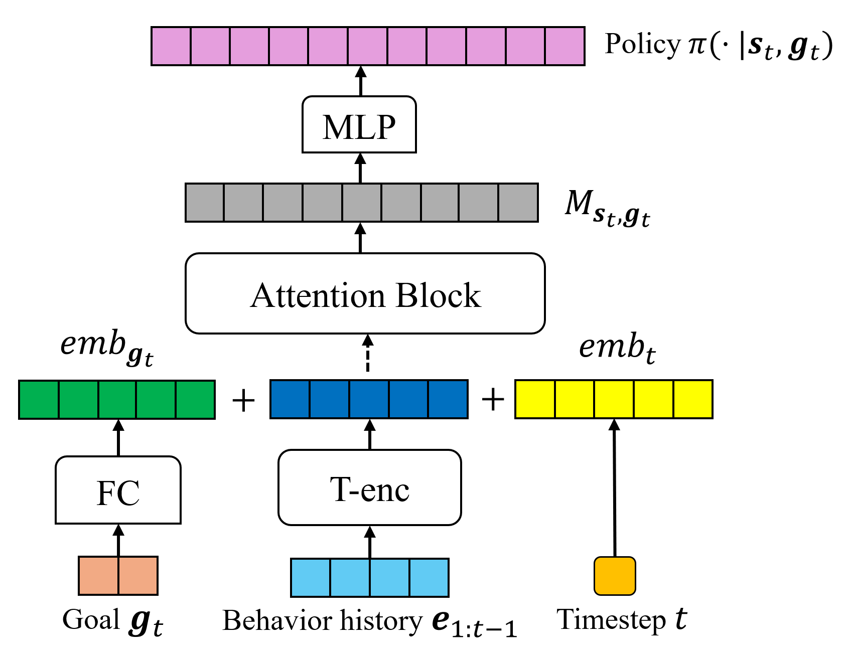
Figure 1: Model structure of MOGCSL.

3.2 MOGCSL Training

The initial step of MOGCSL training is relabeling the training data by substituting the rewards with goals. Specifically, for each trajectory $\tau\in\mathcal{D}_{tr}$, we replace every tuple $(\boldsymbol{s}_{t},a_{t},\boldsymbol{r}_{t})$ with $(\boldsymbol{s}_{t},a_{t},\boldsymbol{g}_{t})$, where $\boldsymbol{g}_{t}$ is defined according to Eq. (1). Subsequently, we employ a sequential model (Kang and McAuley 2018) based on Transformer-encoder (denoted as T-enc) to encode the users’ sequential behaviors and obtain state representations. We chose a transformer-based encoder due to its widely demonstrated capability in sequential recommendation scenarios (Kang and McAuley 2018; Li et al. 2023). However, other encoders, such as GRU or CNN, can also be used. Specifically, let the interaction history of a user up to time $t$ be denoted as $v_{1:t-1}=\{v_{1},...,v_{t-1}\}$. We first map each item $v\in\mathcal{V}$ into the embedding space, resulting in the embedding representation of the history: $\boldsymbol{e}_{1:t-1}=[\boldsymbol{e}_{1},...,\boldsymbol{e}_{t-1}]$. Then we encode $\boldsymbol{e}_{1:t-1}$ by T-enc. Since the current timestep $t$ is also valuable for estimating user’s sequential behavior, we incorporate it via a timestep embedding denoted as $emb_{t}$ through a straightforward embedding table lookup operation. Similarly, we derive the embedding of the goal $emb_{\boldsymbol{g}_{t}}$ through a simple fully connected (FC) layer. The final representation of state $\boldsymbol{s}_{t}$ is derived by concatenating the sequential encoding, timestep embedding and goal embedding together:

$$emb_{\boldsymbol{s}_{t}}=Concat(\emph{T-enc}(\boldsymbol{e}_{1:t-1}),emb_{t},emb_{\boldsymbol{g}_{t}}).$$ (2)

To better capture the mutual information, we further feed the state embedding into a self-attention block:

$$\boldsymbol{M}_{\boldsymbol{s}_{t},\boldsymbol{g}_{t}}=Atten(emb_{\boldsymbol{g}_{t}})).$$ (3)

Then we use an MLP to map the derived embedding into the action space, where each logit represents the preference of taking a specific action (i.e., recommending an item):

$$[\pi_{\theta}(v^{1}|\boldsymbol{s}_{t},\boldsymbol{g}_{t}),...,\pi_{\theta}(v^{N}|\boldsymbol{s}_{t},\boldsymbol{g}_{t})]=\mathbf{\delta}(MLP(\boldsymbol{M}_{\boldsymbol{s}_{t},\boldsymbol{g}_{t}})),$$ (4)

where $v^{i}$ denotes the $i$-th item in the candidate pool, $\mathbf{\delta}$ is the soft-max function, and $\theta$ denotes all parameters of this model. The model structure is shown in Figure 1.

The training objective is to correctly predict the subsequent action that is mostly likely lead to a specific goal given the current state. As discussed in Section 3.1, each trajectory of user’s interaction history represents a successful demonstration of reaching the goal that it actually achieved. As a result, the model can be naturally optimized by minimizing the expected cross-entropy as:

$$\mathcal{L}(\theta)=\mathbb{E}_{(\boldsymbol{s}_{t},a_{t},\boldsymbol{g}_{t})\in\mathcal{D}_{tr}}[-log(\pi_{\theta}(a_{t}|\boldsymbol{s}_{t},\boldsymbol{g}_{t}))].$$ (5)

The training process is illustrated in Algorithm 1.

1Input: training data $\mathcal{D}_{tr}$, batch size $B$, model parameters $\theta$

2 Intialization: initialize parameters $\theta$

3 Relabel all the rewards with goals according to Eq. (1)

4 repeat

5    Randomly sample a batch of $(\boldsymbol{s}_{t},a_{t},\boldsymbol{g}_{t})$ from $\mathcal{D}_{tr}$

6    Compute the representation $\boldsymbol{M}_{\boldsymbol{s}_{t},\boldsymbol{g}_{t}}$ via Eq. (2)-Eq.(3)

7    Derive the prediction logits via Eq. (4)

8    Calculate the loss function $\mathcal{L}(\theta)$ via Eq. (5)

9    Update $\theta$ by minimizing $\mathcal{L}(\theta)$ with stochastic gradient descent: $\theta\leftarrow\theta-\eta\frac{\partial\mathcal{L}(\theta)}{\partial\theta}$

10until convergence

Algorithm 1 Training of MOGCSL

3.3 MOGCSL Inference

After training, we derive a model $\pi_{\theta}(a|\boldsymbol{s},\boldsymbol{g})$ that predicts the next action based on the given state and goal. However, while the goal can be accurately computed through each trajectory in the training data via Eq. (1), we must assign a desirable goal as input for every new state encountered during inference. GCSL approaches typically determine this goal-choosing strategy based on simple statistics calculated from the training data. E.g., Chen et al. (2021) and Zheng, Zhang, and Grover (2022) set the goals for all states at inference as the product of the maximal cumulative reward in training data and a fixed factor serving as a hyperparameter. Similarly, Xin et al. (2023) derive the goals for inference at a given timestep by scaling the mean of the cumulative reward in training data at the same timestep with a pre-defined factor. However, a central yet unexplored question is: what are the general characteristics of the goals and how can we determine them for inference in a principled manner?

In this paper, we investigate the distribution of the goals which can be actually achieved during inference by first stating the following theorem. Proof is given in Appendix A.

Theorem 1.

Assume that the environment is modeled as an MOMDP. Consider a trajectory $\tau$ that is generated by the policy $\pi(a|\boldsymbol{s},\boldsymbol{g})$ given the initial state $\boldsymbol{s}_{1}$ and goal $\boldsymbol{g}_{1}$, the distribution of goals $\boldsymbol{g}^{a}$ (i.e., cumulative rewards) that the agent actually achieves throughout the trajectory is determined by $(\boldsymbol{s}_{1},\boldsymbol{g}_{1},\pi)$.

Based on this theorem, we’d like to learn the distribution of $\boldsymbol{g}^{a}$ conditioned on ($\boldsymbol{s}_{1},\boldsymbol{g}_{1},\pi)$, denoted as $P(\boldsymbol{g}^{a}|\boldsymbol{s}_{1},\boldsymbol{g}_{1},\pi)$. This distribution can be generally learnt by generative models such as GANs (Mirza and Osindero 2014) and diffusion models (Ho and Salimans 2022). In this paper, we propose the use of a conditional variational auto-encoder (CVAE) (Sohn, Lee, and Yan 2015) due to its simplicity, robustness, and ease of formulation.

1Input: state $\boldsymbol{s}^{\prime}$, sample size $K$, policy model $\pi$, utility principle $U$, prior $q(\boldsymbol{g}^{\prime}|\boldsymbol{s}^{\prime})$, distribution of achievable goals $P(\boldsymbol{g}^{a}|\boldsymbol{s}^{\prime},\boldsymbol{g}^{\prime},\pi)$

2 Intialization: set of potential input goals $\boldsymbol{G}^{\prime}=\emptyset$, set of expected achievable goals $\boldsymbol{G}^{a}=\emptyset$

3 for k = $1,\ldots,K$ do

4    Sample a $\boldsymbol{g}^{\prime}_{k}$ from $q(\boldsymbol{g}^{\prime}|\boldsymbol{s}^{\prime})$

5    Compute the expectation of the achievable goal through sampling: $\tilde{\boldsymbol{g}}^{a}_{k}=\mathbb{E}_{\boldsymbol{g}^{a}_{k}\sim P(\cdot|\boldsymbol{s}^{\prime},\boldsymbol{g}^{\prime}_{k},\pi)}\boldsymbol{g}^{a}_{k}$

6    $\boldsymbol{G}^{\prime}=\boldsymbol{G}^{\prime}\cup\boldsymbol{g}^{\prime}_{k}$

7    $\boldsymbol{G}^{a}=\boldsymbol{G}^{a}\cup\tilde{\boldsymbol{g}}^{a}_{k}$

8   

9Choose the best $\tilde{\boldsymbol{g}}^{a}_{b}$ from $\boldsymbol{G}^{a}$ according to $U(\tilde{\boldsymbol{g}}^{a})$

10 Choose corresponding $\boldsymbol{g}^{\prime}_{b}$ from $\boldsymbol{G}^{\prime}$

Return: $\pi(\cdot|\boldsymbol{s}^{\prime},\boldsymbol{g}^{\prime}_{b})$

Algorithm 2 Inference of MOGCSL

This distribution can be learned directly on the training data $\mathcal{D}_{tr}$. Specifically, for each $(\boldsymbol{s},\boldsymbol{g})\in\mathcal{D}_{tr}$ , $\boldsymbol{g}$ should be a sample from the distribution of the achievable goals by the policy $\pi$, given the initial state $\boldsymbol{s}$ and input goal $\boldsymbol{g}$. That’s because the policy $\pi$ is trained to imitate the actions demonstrated by each data point in $\mathcal{D}_{tr}$, where the achieved goal of the trajectory starting from $(\boldsymbol{s},\boldsymbol{g})$ is exactly $\boldsymbol{g}$. Let $\boldsymbol{c}=(\boldsymbol{s},\boldsymbol{g},\pi)$. The loss function is:

$$\begin{split}\mathcal{L}_{CVAE1}=&\mathbb{E}_{(\boldsymbol{s},\boldsymbol{g})\in\mathcal{D}_{tr},z\sim Q_{1}}[logP_{1}(\boldsymbol{g}|z,\boldsymbol{c})+\\ &D_{KL}(Q_{1}(z|\boldsymbol{g},\boldsymbol{c})||P(z))],\end{split}$$ (6)

where $Q_{1}(z|\boldsymbol{g},\boldsymbol{c})$ is the encoder and $P_{1}(\boldsymbol{g}|z,\boldsymbol{c})$ is the decoder. Based on Gaussian distribution assumption, they can be written as $Q_{1}=\mathcal{N}(\mu(\boldsymbol{g},\boldsymbol{c}),\Sigma(\boldsymbol{g},\boldsymbol{c}))$ and $P_{1}=\mathcal{N}(f_{CVAE1}(z,\boldsymbol{c}),\sigma^{2}I)$ respectively, where $z\sim\mathcal{N}(0,I)$. Then we can derive a sample of $\boldsymbol{g}^{a}$ by inputting a sampled $z$ into $f_{CVAE1}$.

On the inference stage, given a new state $\boldsymbol{s}^{\prime}$, we first sample a set of goals $\boldsymbol{g}^{\prime}$ as the possible input of $\pi$ through a learnable prior $q(\boldsymbol{g}^{\prime}|\boldsymbol{s}^{\prime})$. Similarly, we learn this prior via another CVAE on the training data. The loss is:

$$\begin{split}\mathcal{L}_{CVAE2}=&\mathbb{E}_{(\boldsymbol{s},\boldsymbol{g})\in\mathcal{D}_{tr},z\sim Q_{2}}[logP_{2}(\boldsymbol{g}|z,\boldsymbol{s})+\\ &D_{KL}(Q_{2}(z|\boldsymbol{g},\boldsymbol{s})||P(z))].\end{split}$$ (7)

Finally, we’ll choose a desirable goal as the input along with the new state $\boldsymbol{s}^{\prime}$ encountered in inference by sampling from the two CVAE models. Specifically, we propose to: (1) sample from the prior $q(\boldsymbol{g}^{\prime}|\boldsymbol{s}^{\prime})$ to get a set of potential input goals, denoted as $\boldsymbol{G}^{\prime}$, (2) for each $\boldsymbol{g}^{\prime}\in\boldsymbol{G}^{\prime}$, estimate the expectation of the actually achievable goal $\tilde{\boldsymbol{g}}^{a}$ by sampling from $P(\cdot|\boldsymbol{s}^{\prime},\boldsymbol{g}^{\prime},\pi)$ and taking the average, (3) choose a best goal as input for inference from $\boldsymbol{G}^{\prime}$ according to the associated expected $\tilde{\boldsymbol{g}}^{a}$ by a predefined utility principle $U(\tilde{\boldsymbol{g}}^{a})$, which generally tends to pick up a “high” goal. See Algorithm 2 for detailed inference pseudocode.

3.4 Analysis of Denoising Capability

An important benefit of MOGCSL is its capability to remove harmful effects of potentially noisy instances in the training data. To illustrate this, we consider the following setup that is common in recommender systems. There is a recommender system that has been operational, and recording data. At each interaction, the system shows the user a short list of items. The user then chooses one of these items. In the counterfactual that the recommender system is ideal, the action recorded would be $a$ which reveals the user’s true interest. Since the actual recommender system to collect the data is not ideal, we have no direct access to $a$, but rather to a noisy version of it $\varepsilon(a)$. We also record a long-term and multidimensional goal (e.g., the cumulative reward) $\boldsymbol{g}=(g_{1},...,g_{n})$ at each interaction (known only at the end of the session, but recorded retroactively). Thus our training data is a sample from a distribution $\mathcal{D}$ of tuples $(\boldsymbol{s},\boldsymbol{g},\varepsilon(a))$.

We assume that the noisy portion of the training data originates from users who are presented with a list of items that are not suitable for them, rendering their reactiongs to these recommendations uninformative. Conversely, interactions achieving higher goals are generally less noisy, meaning $\varepsilon(a)$ is closer to $a$. To illustrate this, consider a scenario where a user clicks two recommended items ($v_{1}$ and $v_{2}$) under the same state. After clicking $v_{1}$, the user chooses to quit the system, while he stays longer and browses more items after clicking $v_{2}$. This indicates that the goal (i.e., cumulative reward) with $v_{2}$ is larger than that with $v_{1}$. In this case, we argue that $v_{2}$ should be considered as the user’s truly preferred item over $v_{1}$. That’s because the act of quitting, which results in a smaller goal, indicates user dissatisfaction with the current recommendation, although he did click $v_{2}$ at the current step. Our proposed MOGCSL can model and leverage this mechanism based on multi-dimensional goals, which serve as a description of the future effects of current actions on multiple objectives. In other words, MOGCSL tends to prioritize instances that result in high achievable goals on multiple objectives, while discounting those with low goals. Specifically, by incorporating multi-dimensional goals as input, MOGCSL can effectively differentiate between noisy and noiseless samples in the training data. During inference, when high goals are specified as input, the model can make predictions based primarily on the patterns learned from the corresponding noiseless interaction data.

To empirically show its effect, we conduct experiments that are illustrated in Appendix B.1 due to limited space. The results demonstrate the denoising capability of MOGCSL.

4 Experiments

In this section, we introduce our experiments on two e-commerce datasets, aiming to address the following research questions: 1) RQ1. How does MOGCSL perform when compared to previous methods for multi-objective learning in recommender systems? 2) RQ2. How does MOGCSL mitigate the complexity challenges, including space and time complexity, as well as the intricacies of parameter tuning encountered in prior research? 3) RQ3. How does the goal-generation module for inference perform when compared to strategies based on simple statistics?

4.1 Experimental Setup

Datasets We conduct experiments on two publicly available datasets: RetailRocket and Challenge15. Both of them include binary labels indicating whether a user clicked or purchased the currently recommended item.

Baselines As introduced before, prior research on multi-objective learning encompass both model structure adaptation and optimization constraints. In our experiments, we consider two representative model architectures: Shared-Bottom and MMOE (Ma et al. 2018). For works focusing on studying optimization constraints, We compare three methods: Fixed-Weights (Wang et al. 2016) directly assigns fixed weights for different objectives based on grid search; DWA (Liu, Johns, and Davison 2019) aims to dynamically assign weights by considering the dynamics of loss change; PE (Lin et al. 2020) is designed for generating Pareto-efficient recommendations across multiple objectives.

Following previous research(Yu et al. 2020), we consider all these optimization methods for each model architecture, resulting in six baselines denoted as Share-Fix, Share-DWA, Share-PE, MMOE-Fix, MMOE-DWA, MMOE-PE. Additionally, we introduce a variant of a recent work called PRL (Xin et al. 2023), which firstly applied GCSL to recommender systems. Specifically, similar to classic multi-objective methods, we compute the weighted summation of rewards from all objectives at each timestep. Then the goal is derived by the overall cumulative reward as a scalar following conventional GCSL. We call this variant as MOPRL. Since we formulate our problem as an MOMDP, we also incorporate a baseline called SQN (Xin et al. 2020) that applies offline reinforcement learning for sequential recommendation. Similarly, the aggregate reward is derived by the weighted summation of all objective rewards.

To ensure a fair comparison, we employ the T-enc and self-attention block introduced in Section 3.2 as the base module to encode sequential data for all compared baselines.

Evaluation Metrics We employ two widely recognized information retrieval metrics to evaluate model performance in top-$k$ recommendation: hit ratio (HR@$k$) and normalized discounted cumulative gain (NDCG@$k$).

More details about the datasets, baselines, metrics, and implementation can be found in Appendix B.

Table 1: Comparison between MOGCSL and other baselines on RetailRocket and Challenge15. The mean and standard deviation over 5 seeds are reported. Boldface denotes the best results.

[RetailRocket]	Purchase (%)				Click (%)
	HR@10	NDCG@10	HR@20	NDCG@20	HR@10	NDCG@10	HR@20	NDCG@20
Share-Fix	48.57$\pm$0.17	45.79$\pm$0.09	49.47$\pm$0.10	46.01$\pm$0.08	35.51$\pm$0.24	25.85$\pm$0.16	40.15$\pm$0.20	27.03$\pm$0.14
Share-DWA	48.11$\pm$0.04	45.83$\pm$0.08	48.64$\pm$0.08	45.96$\pm$0.06	34.20$\pm$0.27	25.53$\pm$0.12	38.43$\pm$0.31	26.60$\pm$0.13
Share-PE	48.67$\pm$0.12	45.94$\pm$0.03	49.42$\pm$0.04	46.13$\pm$0.02	35.69$\pm$0.08	26.20$\pm$0.08	40.28$\pm$0.11	27.37$\pm$0.07
MMOE-Fix	47.74$\pm$0.09	44.01$\pm$0.05	48.61$\pm$0.11	44.23$\pm$0.04	35.29$\pm$0.16	25.67$\pm$0.09	40.04$\pm$0.26	26.87$\pm$0.11
MMOE-DWA	47.78$\pm$0.40	44.57$\pm$0.13	48.44$\pm$0.24	44.79$\pm$0.09	35.68$\pm$0.46	26.13$\pm$0.29	40.22$\pm$0.57	27.28$\pm$0.32
MMOE-PE	46.58$\pm$0.22	43.72$\pm$0.15	47.37$\pm$0.11	43.94$\pm$0.14	35.39$\pm$0.27	26.19$\pm$0.11	39.78$\pm$0.39	27.31$\pm$0.14
SQN	62.03$\pm$0.31	48.06$\pm$0.24	66.19$\pm$0.28	49.14$\pm$0.19	33.02$\pm$0.47	22.79$\pm$0.25	38.03$\pm$0.48	24.06$\pm$0.32
MOPRL	61.18$\pm$0.19	50.74$\pm$0.10	64.76$\pm$0.25	51.65$\pm$0.02	33.99$\pm$0.11	24.31$\pm$0.08	38.98$\pm$0.08	25.57$\pm$0.08
MOGCSL	65.43$\pm$0.15	52.92$\pm$0.11	69.28$\pm$0.14	53.90$\pm$0.14	36.30$\pm$0.25	25.24$\pm$0.15	41.92$\pm$0.55	26.67$\pm$0.19

[Challenge15]	Purchase (%)				Click (%)
	HR@10	NDCG@10	HR@20	NDCG@20	HR@10	NDCG@10	HR@20	NDCG@20
Share-Fix	38.18$\pm$0.10	25.47$\pm$0.26	43.97$\pm$0.18	26.93$\pm$0.20	41.61$\pm$0.30	25.77$\pm$0.16	49.19$\pm$0.43	27.70$\pm$0.19
Share-DWA	38.27$\pm$0.18	25.63$\pm$0.08	43.95$\pm$0.19	27.07$\pm$0.08	41.49$\pm$0.24	25.90$\pm$0.16	48.90$\pm$0.20	27.77$\pm$0.14
Share-PE	38.92$\pm$0.09	25.83$\pm$0.13	44.82$\pm$0.12	27.32$\pm$0.07	42.46$\pm$0.16	26.39$\pm$0.06	50.05$\pm$0.17	28.32$\pm$0.06
MMOE-Fix	35.34$\pm$0.12	23.87$\pm$0.07	40.68$\pm$0.09	25.22$\pm$0.12	43.82$\pm$0.16	27.33$\pm$0.09	51.42$\pm$0.19	29.26$\pm$0.10
MMOE-DWA	37.04$\pm$0.40	24.88$\pm$0.13	42.64$\pm$0.24	26.30$\pm$0.09	42.20$\pm$0.46	26.45$\pm$0.29	49.48$\pm$0.57	28.30$\pm$0.32
MMOE-PE	36.40$\pm$0.36	24.66$\pm$0.19	41.52$\pm$0.33	25.96$\pm$0.19	44.04$\pm$0.09	27.44$\pm$0.03	51.60$\pm$0.07	29.37$\pm$0.03
SQN	55.05$\pm$0.42	34.35$\pm$0.28	64.42$\pm$0.53	36.74$\pm$0.34	42.55$\pm$0.35	25.80$\pm$0.23	50.66$\pm$0.32	27.86$\pm$0.26
MOPRL	54.79$\pm$0.37	35.37$\pm$0.26	63.10$\pm$0.45	37.49$\pm$0.27	42.14$\pm$0.21	25.62$\pm$0.18	50.18$\pm$0.25	27.66$\pm$0.19
MOGCSL	56.82$\pm$0.25	35.93$\pm$0.15	65.64$\pm$0.55	38.17$\pm$0.19	42.47$\pm$0.15	25.64$\pm$0.11	50.52$\pm$0.14	27.73$\pm$0.11

4.2 Performance Comparison (RQ1)

We begin by conducting experiments to compare the performance of MOGCSL and selected baselines. The experimental results are presented in Table 1. It’s worth mentioning that a straightforward strategy based on training set statistics is employed to determine the inference goals in PRL (Xin et al. 2023). Specifically, at each timestep in inference, the goal are set as the average cumulative reward from offline data at the same timestep, multiplied by a hyper-parameter factor $\lambda$ that is tuned using the validation set. To ensure a fair and meaningful comparison, we adopt the same strategy here for determining inference goals in MOGCSL. The comparison between different goal-choosing strategies is discussed in Section 4.4.

On RetailRocket, MOGCSL significantly outperforms previous multi-objective benchmarks in terms of purchase-related metrics. Regarding click metrics, MOGCSL achieves the best performance on HR, while Share-PE slightly outperforms it on NDCG. However, the performance gap between Share-PE and MOGCSL for purchase-related metrics ranges from 17% to 20%, whereas Share-PE only marginally outperforms MOGCSL on NDCG for purchase by less than 1%. Additionally, we observe that the more complex architecture design, MMOE, performs worse than the simpler Shared-Bottom structure. Surprisingly, a naive optimization strategy based on fixed loss weights can outperform more advanced methods like DWA across several metrics (e.g., Share-Fix vs Share-DWA). These findings highlight the limitations of previous approaches that rely on assumptions about model architectures or optimization constraints, which may not be necessarily true under certain environments. Similar trends are observed on Challenge15. While MMOE-PE performs slightly better on click metrics by 1-2%, MOGCSL achieves a substantial performance improvement on the more important purchase metrics by 11-20%.

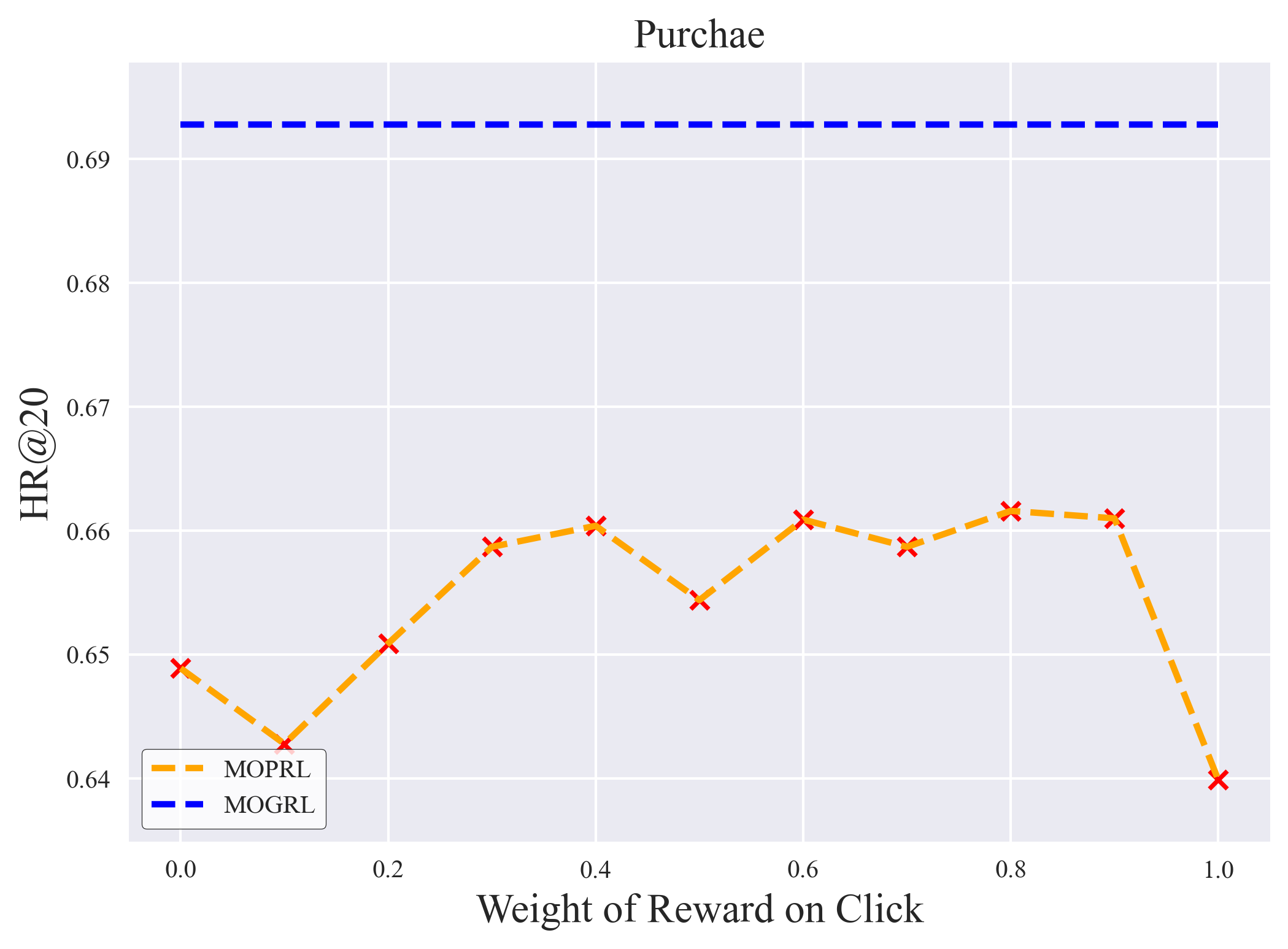
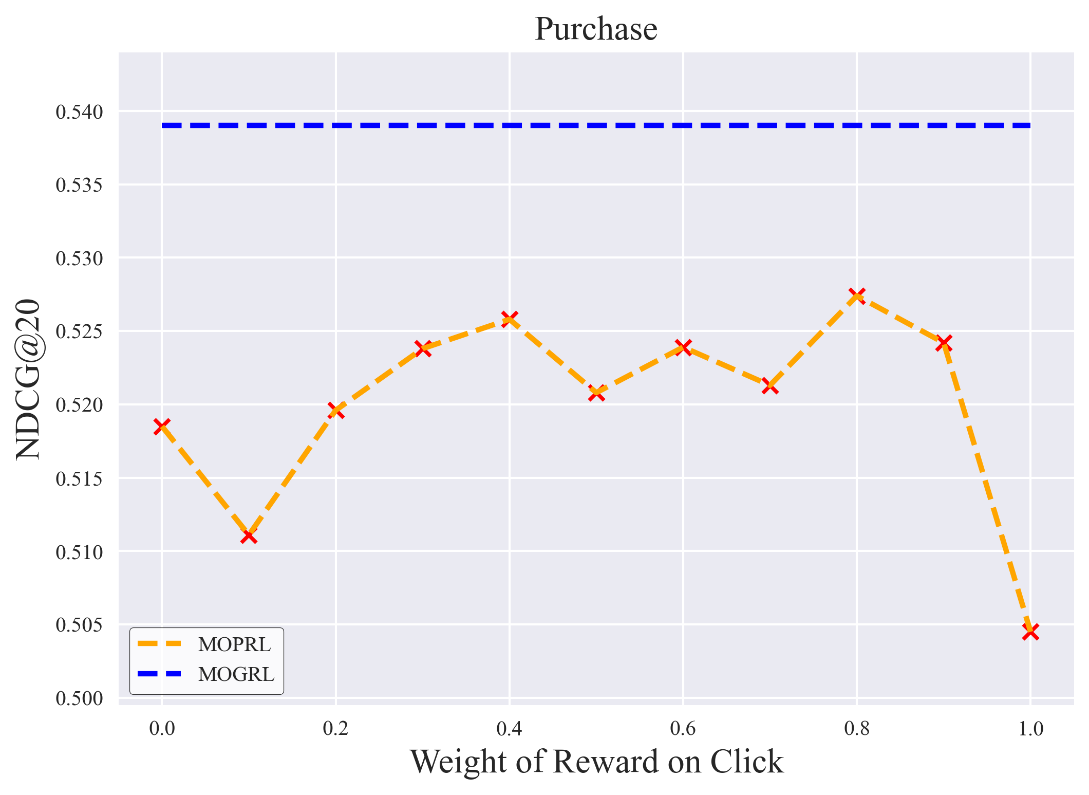
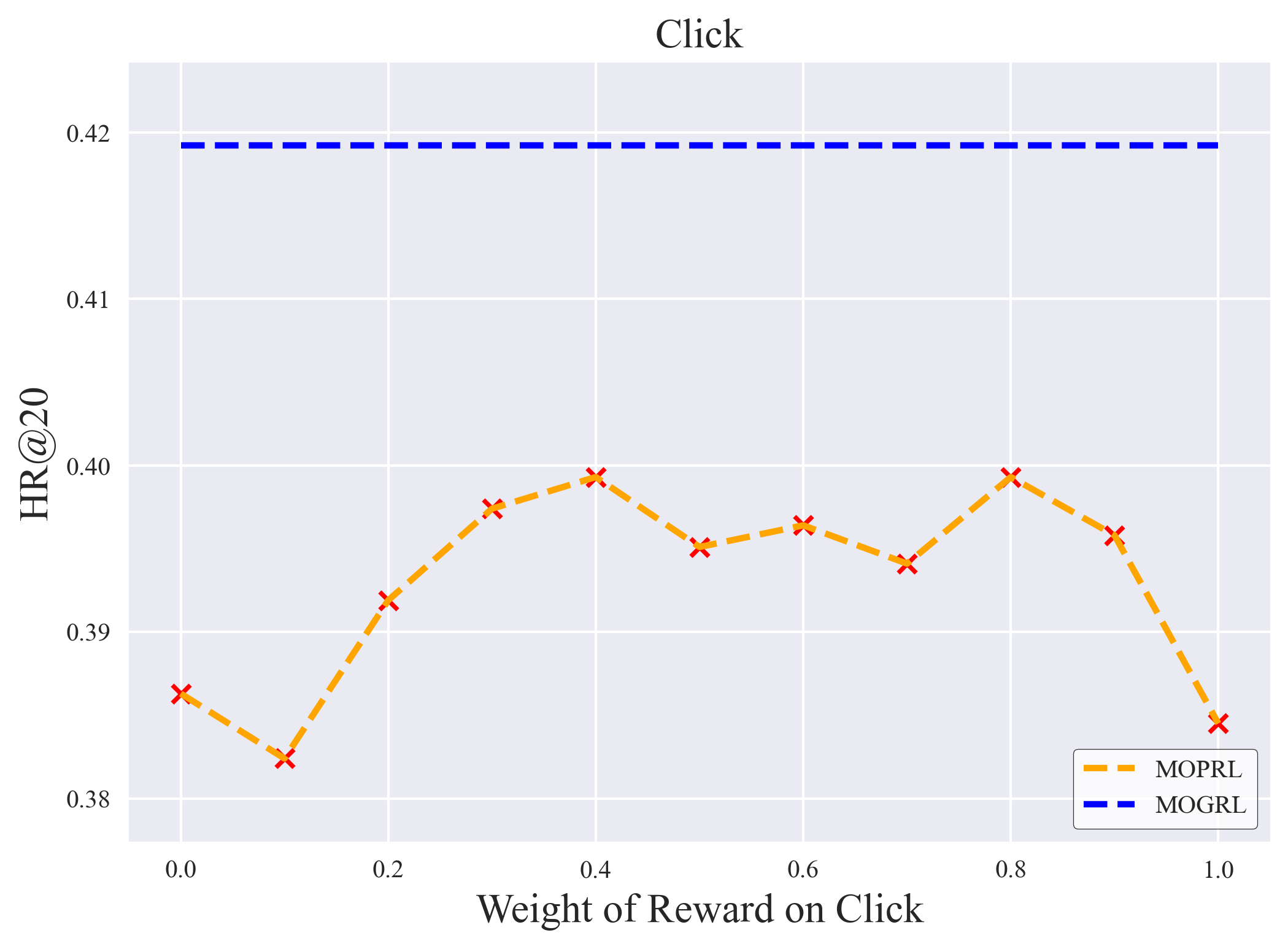
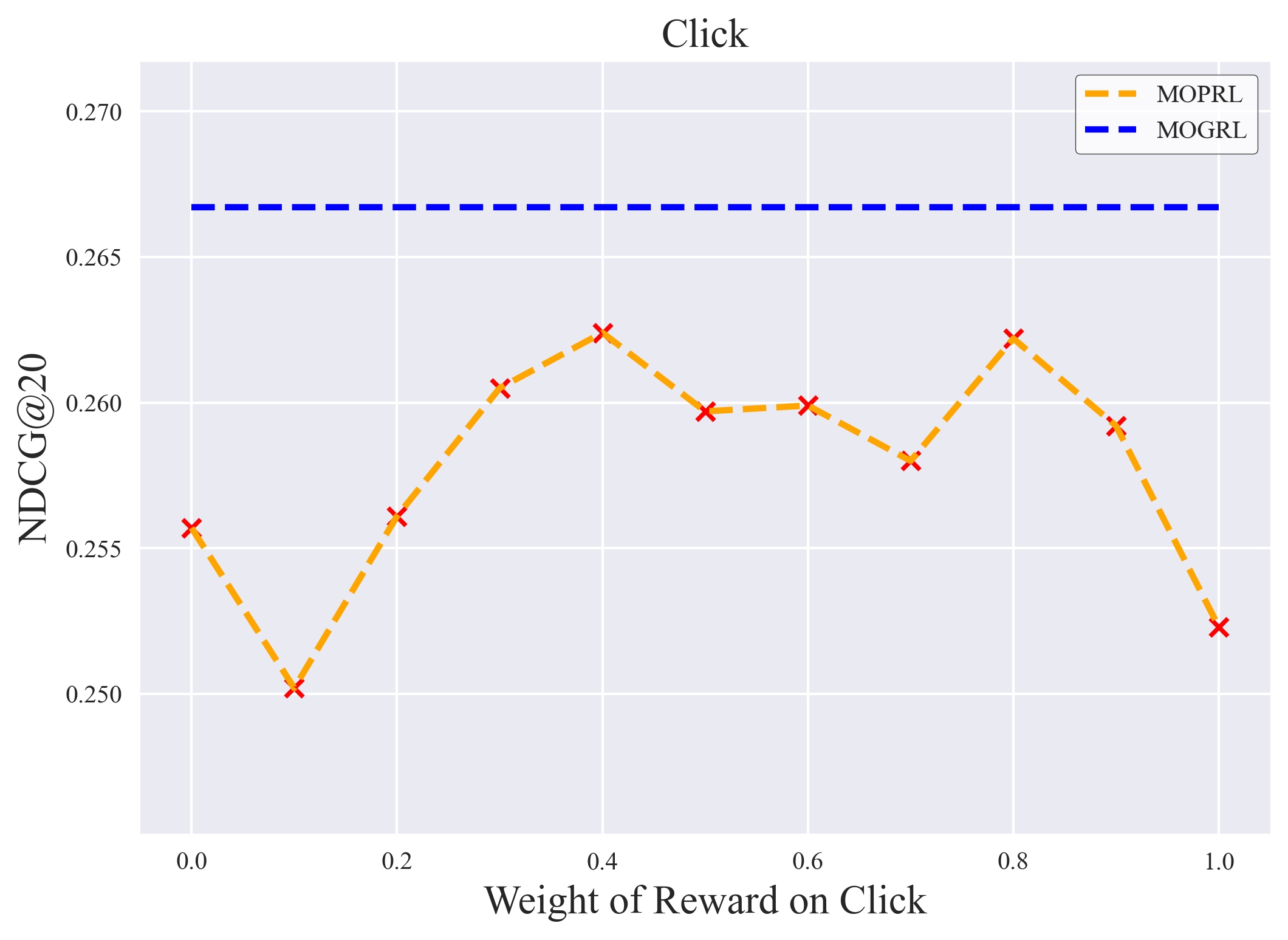
Figure 2: Comparison between MOGCSL and MOPRLs with different weight combinations on RetailRocket.

Apart from previous benchmarks for multi-objective learning, MOGCSL also exhibits significant and consistent performance improvements on both datasets compared to offline RL based SQN and the variant MOPRL created on standard GCSL. Especially, at each timestep, the overall reward of them is calculated as the weighted sum of rewards across all objectives. In our experiments, it’s defined as $r^{\prime}=w_{c}r^{c}+w_{p}r^{p}$, where $r^{c}$ and $r^{p}$ are click and purchase reward and $w_{c}+w_{p}=1$. Then the goal in MOPRL is derived by calculating the cumulative rewards as a scalar. In contrast, MOGCSL takes the goal as a vector, allowing the disentanglement of rewards for different objectives along different dimensions. Notably, no additional summation weights or other constraints are required. We have conducted experiments to compare the performance of MOGCSL to MOPRLs with different weight combinations. Figure 2 shows the performance comparison on the RetailRocket dataset. Results on Challenge15 exhibit similar trends. It’s clear that MOGCSL consistently outperforms MOPRL across all weight combinations on both click and purchase metrics, demonstrating that representing the goal as a multi-dimensional vector enhances the effectiveness of GCSL on multi-objective learning.

4.3 Complexity Comparison (RQ2)

Apart from the performance improvement, MOGCSL also benefits from seamless integration with classic sequential models and optimization by standard cross-entropy loss, adding minimal additional complexity. During the training stage, the only extra complexity arises from relabeling one-step rewards with goals and including them as input to the sequential model. In contrast, previous multi-objective learning methods often introduce significantly excess time and space complexity (Zhang and Yang 2021). For instance, MMOE and Shared-Bottom both design separate towers for each objective, resulting in dramatic increase in model parameters. SQN needs an additional RL head for optimization on TD error. DWA requires recording and calculating loss change dynamics for each training epoch, while PE involves computing the inverse of a large parameter matrix to solve an optimization problem under KKT conditions. Additionally, tuning the combination of weights for multiple objectives using grid search for Fix-Weight, SQN, and MOPRL is time-consuming. Approximately $O(m^{n})$ repetitive experiments are needed to find the nearly optimal weight combination, where $m$ denotes the size of the search space per dimension and $n$ represents the number of objectives.

Table 2 summarizes the complexity comparison. It’s evident that MOGCSL significantly benefits from a smaller model size and faster training speed, while concurrently achieving great recommendation performance.

Table 2: Comparison of time and space complexity. The training time is calculated on RetailRocket.

	Model	Training time	Training time
	Size	(per epoch)	(total)
Share-Fix	14.0M	137.2s	9.6Ks
Share-DWA	14.0M	141.7s	5.3Ks
Share-PE	14.0M	1364.3s	55.6Ks
MMOE-Fix	14.1M	148.7s	10.2Ks
MMOE-DWA	14.1M	152.2s	9.5Ks
MMOE-PE	14.1M	3120.5s	60.5Ks
SQN	11.3M	175.7s	10.5Ks
MOPRL	9.1M	116.9s	3.4Ks
MOGCSL	9.1M	117.2s	3.0Ks

4.4 Goal-Choosing Strategy Comparison (RQ3)

As introduced in Section 3.3, most previous research on GCSL decides the inference goals based on simple statistics on the training set. However, we demonstrate that the distribution of the goals achieved by the agent during inference should be jointly determined by the initial state, input goal and behavior policy. Based on that, we propose a novel algorithm (see Algorithm 2) that leverages CVAE to derive feasible and desirable goals for inference. Note that an utility principle $U(\boldsymbol{g})$ is required to evaluate the goodness of the multi-dimensional goals, which is generally preferable for “high” goals but could be flexible with specific business requirements. In our experiments, we select the best goal $\tilde{\boldsymbol{g}}^{a}_{b}$ from the set $\boldsymbol{G}^{a}$ based on the following rule:

$$\tilde{\boldsymbol{g}}^{a}_{b}=\tilde{\boldsymbol{g}}\in\boldsymbol{G}^{a},\;\mathrm{s.t.}\ \nexists\,\tilde{\boldsymbol{g}}^{\prime}\in\boldsymbol{G}^{a}\setminus\tilde{\boldsymbol{g}}\,,\ \tilde{g}^{\prime}_{i}\geq\tilde{g}_{i}\ \forall i\in[1,d].$$ (8)

We compare two variants of MOGCSL here. MOGCSL-S employs the statistical strategy introduced in Section 4.2, while MOGCSL-C utilizes the goal-choosing method based on CVAE (Algorithm 2). Due to limited space, we’ve included the result table in Appendix 4. Surprisingly, we observe that these two strategies do not significantly differ in overall performance across both datasets. While MOGCSL-C performs slightly better on RetailRocket, it exhibits worse performance on Challenge15. To investigate the reason, we conduct an additional experiment by varying the factor $\lambda$ for the inference goals of MOGCSL-S. The results reveals that the optimal performance is achieved when the factor is set between 1 and 2 for all metrics. When it grows larger, performance consistently declines. The figure is shown in Appendix B.7. Interestingly, similar findings have been reported in prior research (Chen et al. 2021; Xin et al. 2023; Zheng, Zhang, and Grover 2022), demonstrating that setting large inference goals can actually harm performance.

We posit that the sparsity of training data within the high-goal space may contribute to the suboptimal performance of more advanced goal-choosing methods. While we may find some potentially achievable high goals, the model lacks sufficient training data to learn effective actions to reach these goals. Notably, the mean cumulative reward across all trajectories in both datasets is only around 5.3 for click and 0.2 for purchase. Consequently, most training data demonstrates how to achieve relatively low goals, hindering the model’s ability to generalize effectively for larger goals in inference.

The results provide several insights for selecting goal-choosing strategies when applying MOGCSL in practical applications. First, strategies based on simple statistics on the training data prove to be efficient and effective in many cases, particularly when low latency or reduced model complexity is required during inference. Second, if we aim to further enhance performance using more advanced goal-choosing algorithms, access to a training set with more instances with high-valued goals could be crucial.

5 Conclusion

We propose a novel framework named MOGCSL for multi-objective recommendation. MOGCSL utilizes a vectorized goal to disentangle the representation of different objectives. It benefits from the ability to adapt to general architectures and standard optimization patterns. Also, MOGCSL is able to distinguish and eliminate harmful effects from the potentially highly noisy portions of the training data often prevalent in recommender systems. Besides, we propose a novel goal-choosing algorithm to model and determine desirable goals for inference of MOGCSL. Extensive experiments validate the superiority of MOGCSL in terms of both performance and efficiency. We aim to also study the applicability of the MOGCSL framework to other domains that have significant amounts of uninformative data that one is better off ignoring while building a predictive model.

Appendix A Proof of Theorem 1

First, as introduced in Section 3.1, we formulate our problem as an MOMDP (Roijers et al. 2013) described by the tuple $<\mathcal{S},\mathcal{A},T,R,\rho>$ given an environment that the agent can interact with. Especially, in our problem setting, the environment is taken as all the users on the platform and the agent is the recommender system. A state $\boldsymbol{s}_{t}\in\mathcal{S}$ is taken as the representation of user’s preferences at a given timestep $t$. The action space $\mathcal{A}$ includes all candidate items to be recommended. $T(\boldsymbol{s}_{t+1}|\boldsymbol{s}_{t},a_{t})$ determines the state transition probability. $R(s_{t},a_{t})$ is the reward function, where $\boldsymbol{r}_{t}=R(s_{t},a_{t})$ means the agent receives a reward $\boldsymbol{r}_{t}$ after taking an action $a_{t}$ under state $\boldsymbol{s}_{t}$. $\rho$ is the distribution of the initial states.

Then we begin by first proving the following lemma.

Lemma A.1.

Assume that the environment is modeled as an MOMDP. Consider a trajectory $\tau$ that is generated by the policy $\pi(a|\boldsymbol{s},\boldsymbol{g})$ given the initial state $\boldsymbol{s}_{1}$ and goal $\boldsymbol{g}_{1}$, the distributions of $\boldsymbol{s}_{t}$ and $(\boldsymbol{s}_{t}$, $\boldsymbol{g}_{t})$ at each timestep are both determined by $(\boldsymbol{s}_{1},\boldsymbol{g}_{1},\pi)$.

Proof.

First, for $t=1$ we have:

$$\mathrm{Pr}(\boldsymbol{r}_{1}=\boldsymbol{r})=\sum_{a}\mathds{1}({R}(\boldsymbol{s}_{1},a)=\boldsymbol{r})\pi(a|\boldsymbol{s}_{1},\boldsymbol{g}_{1}).$$ (9)

Note that the reward function ${R}(\boldsymbol{s},a)$ is fixed for the given environment. Then, we complete the proof by mathematical induction.
Statement:The distributions of $\boldsymbol{s}_{t}$ and $(\boldsymbol{s}_{t}$, $\boldsymbol{g}_{t})$ are both determined by $(\boldsymbol{s}_{1},\boldsymbol{g}_{1},\pi)$, for $t=2,3,...,|\tau|$.
Base case $t=2$: Since $\boldsymbol{s}_{1}$ and $\boldsymbol{g}_{1}$ are given and fixed, we have:

$$\mathrm{Pr}(\boldsymbol{s}_{2}=\boldsymbol{s})=\sum_{a}T(\boldsymbol{s}|a,\boldsymbol{s}_{1})\pi(a|\boldsymbol{s}_{1},\boldsymbol{g}_{1}).$$ (10)

It’s clear that $\boldsymbol{s}_{2}\sim f_{s_{2}}(\boldsymbol{s};\boldsymbol{s}_{1},\boldsymbol{g}_{1},\pi)$ where $f_{s_{2}}$ is a distribution determined by $(\boldsymbol{s}_{1},\boldsymbol{g}_{1},\pi)$.

For $(\boldsymbol{s}_{2},\boldsymbol{g}_{2})$, according the definition of $\boldsymbol{g}_{t}$ in Eq. (1), when a reward $\boldsymbol{r}_{t}$ is received, the desired goal on next timestep is $\boldsymbol{g}_{t+1}=\boldsymbol{g}_{t}-\boldsymbol{r}_{t}$. Combined with Eq. (9), We have:

$$\begin{split}\mathrm{Pr}(\boldsymbol{s}_{2}=\boldsymbol{s},\boldsymbol{g}_{2}=\boldsymbol{g})=\sum_{a}\mathds{1}({R}(\boldsymbol{s}_{1},a)=\boldsymbol{g}_{1}-\boldsymbol{g})\cdot\\ T(\boldsymbol{s}|\boldsymbol{s}_{1},a)\pi(a|\boldsymbol{s}_{1},\boldsymbol{g}_{1}).\end{split}$$ (11)

Since the dynamic function $T(\boldsymbol{s}^{\prime}|\boldsymbol{s},a)$ is given, it’s clear that $(\boldsymbol{s}_{2},\boldsymbol{g}_{2})\sim f_{s_{2},g_{2}}(\boldsymbol{s},\boldsymbol{g};\boldsymbol{s}_{1},\boldsymbol{g}_{1},\pi)$.
Inductive Hypothesis: Suppose the statement holds for all $t$ up to some $n$, $2\leq n\leq|\tau|-1$.
Inductive Step: Let $t=n+1$, similar to the base case, we have:

$$\begin{split}\mathrm{Pr}(\boldsymbol{s}_{n+1}=\boldsymbol{s})=\sum_{a^{\prime},\boldsymbol{s}^{\prime},\boldsymbol{g}^{\prime}}T(\boldsymbol{s}|\boldsymbol{s}^{\prime},a^{\prime})\pi(a^{\prime}|\boldsymbol{s}^{\prime},\boldsymbol{g}^{\prime})\cdot\\ \mathrm{Pr}(\boldsymbol{s}_{n}=\boldsymbol{s}^{\prime},\boldsymbol{g}_{n}=\boldsymbol{g}^{\prime}).\end{split}$$ (12)

$$\begin{split}\mathrm{Pr}(\boldsymbol{s}_{n+1}=\boldsymbol{s},\boldsymbol{g}_{n+1}=\boldsymbol{g})=\sum_{a^{\prime},\boldsymbol{s}^{\prime},\boldsymbol{g}^{\prime}}[\mathds{1}({R}(\boldsymbol{s}^{\prime},a^{\prime})=\boldsymbol{g}^{\prime}-\boldsymbol{g})\cdot\\ T(\boldsymbol{s}|\boldsymbol{s}^{\prime},a^{\prime})\pi(a^{\prime}|\boldsymbol{s}^{\prime},\boldsymbol{g}^{\prime})\mathrm{Pr}(\boldsymbol{s}_{n}=\boldsymbol{s}^{\prime},\boldsymbol{g}_{n}=\boldsymbol{g}^{\prime})].\end{split}$$ (13)

According to the hypothesis that the distributions of $(\boldsymbol{s}_{n}$, $\boldsymbol{g}_{n})$ is determined by $(\boldsymbol{s}_{1},\boldsymbol{g}_{1},\pi)$, it’s easy to see that $\boldsymbol{s}_{n+1}\sim f_{\boldsymbol{s}_{n+1}}(\boldsymbol{g};\boldsymbol{s}_{1},\boldsymbol{g}_{1},\pi)$ and $(\boldsymbol{s}_{n+1},\boldsymbol{g}_{n+1})\sim f_{s_{n+1},g_{n+1}}(\boldsymbol{s},\boldsymbol{g};\boldsymbol{s}_{1},\boldsymbol{g}_{1},\pi)$.

As a result, the statement holds for $t=n+1$. By the principle of mathematical induction, the statement holds for all $t=2,3,...,|\tau|$. Apparently, that proves Lemma A.1. ∎

Then, based on the lemma, we can prove Theorem 1.

Proof.

Let $|\tau|=T$, by definition we have:

$$\boldsymbol{g}^{a}=\sum_{t=1}^{T}\boldsymbol{r}_{t},$$ (14)

Let $\mathbf{x}_{n}=(\boldsymbol{r}_{n},...,\boldsymbol{r}_{1})$, according to the Markov property and Bayes’ rules we have:

$$\begin{split}P(\boldsymbol{r}_{n}&|\boldsymbol{r}_{n-1},...,\boldsymbol{r}_{1})=P(\boldsymbol{r}_{n}|\mathbf{x}_{n-1})\\ =&\sum_{\boldsymbol{s}_{n}}P(\boldsymbol{r}_{n}|\boldsymbol{s}_{n},\mathbf{x}_{n-1})P(\boldsymbol{s}_{n}|\mathbf{x}_{n-1})\\ =&\sum_{\boldsymbol{s}_{n}}P(\boldsymbol{r}_{n}|\boldsymbol{s}_{n})\sum_{\boldsymbol{s}_{n-1}}P(\boldsymbol{s}_{n}|\boldsymbol{s}_{n-1},\mathbf{x}_{n-1})P(\boldsymbol{s}_{n-1}|\mathbf{x}_{n-1})\\ =&\sum_{\boldsymbol{s}_{n}}P(\boldsymbol{r}_{n}|\boldsymbol{s}_{n})\sum_{\boldsymbol{s}_{n-1}}P(\boldsymbol{s}_{n}|\boldsymbol{s}_{n-1},\mathbf{x}_{n-1})...\\ &\sum_{\boldsymbol{s}_{2}}P(\boldsymbol{s}_{3}|\boldsymbol{s}_{2},\mathbf{x}_{n-1})P(\boldsymbol{s}_{2}|\mathbf{x}_{n-1})\\ \end{split}$$ (15)

For the first term, we have:

$$P(\boldsymbol{r}_{n}|\boldsymbol{s}_{n})=\sum_{a_{n},\boldsymbol{g}_{n}}\frac{\mathds{1}({R}(\boldsymbol{s}_{n},a_{n})=\boldsymbol{r}_{n})\pi(a_{n}|\boldsymbol{s}_{n},\boldsymbol{g}_{n})P(\boldsymbol{s}_{n},\boldsymbol{g}_{n})}{P(\boldsymbol{s}_{n})}.$$ (16)

Since $(\boldsymbol{s}_{1},\boldsymbol{g}_{1})$ is given and fixed, for each $m\in[2,n-1]$ we have:

$$\begin{split}P(\boldsymbol{s}_{m+1}|\boldsymbol{s}_{m},\mathbf{x}_{n-1})=\sum_{a_{m}}\pi(a_{m}|\boldsymbol{s}_{m},\boldsymbol{g}_{1}-\sum_{i=1}^{m-1}\boldsymbol{r}_{i})\cdot\\ T(\boldsymbol{s}_{m+1}|\boldsymbol{s}_{m},a_{m})\mathds{1}[R(\boldsymbol{s}_{m},a_{m})=\boldsymbol{r}_{m}].\end{split}$$ (17)

Similarly, the last term can be written as:

$$P(\boldsymbol{s}_{2}|\mathbf{x}_{n-1})=\sum_{a_{1}}\pi(a_{1}|\boldsymbol{s}_{1},\boldsymbol{g}_{1})T(\boldsymbol{s}_{2}|\boldsymbol{s}_{1},a_{1})\mathds{1}[R(\boldsymbol{s}_{1},a_{1})=\boldsymbol{r}_{1}].$$ (18)

According to Lemma A.1, the distributions of $\boldsymbol{s}_{n}$ and $(\boldsymbol{s}_{n},\boldsymbol{g}_{n})$ are both determined by $(\boldsymbol{s}_{1},\boldsymbol{g}_{1},\pi)$. As a result, by Eq. (15 - 18), it’s clear that the distribution of the conditional probability distribution $P(\boldsymbol{r}_{n+1}|\boldsymbol{r}_{n},...,\boldsymbol{r}_{1})$ is also determined by $(\boldsymbol{s}_{1},\boldsymbol{g}_{1},\pi)$. Then, the distribution of $\boldsymbol{g}^{a}$ can be written as:

$$\begin{split}&\mathrm{Pr}(\boldsymbol{g}^{a}=\boldsymbol{g})=\idotsint_{\sum_{i=1}^{T}\boldsymbol{r}_{i}=\boldsymbol{g}}f(\boldsymbol{r}_{1},\boldsymbol{r}_{2},...,\boldsymbol{r}_{T})d\boldsymbol{r}_{1}d\boldsymbol{r}_{2}...d\boldsymbol{r}_{T}\\ &=\idotsint_{\sum_{i=1}^{T}\boldsymbol{r}_{i}=\boldsymbol{g}}f_{1}(\boldsymbol{r}_{1})f_{2}(\boldsymbol{r}_{2}|\boldsymbol{r}_{1})...f_{T}(\boldsymbol{r}_{T}|\boldsymbol{r}_{T-1},...,\boldsymbol{r}_{1})d\boldsymbol{r}_{1}...d\boldsymbol{r}_{T}\end{split}$$ (19)

Obviously, the distribution of $\boldsymbol{g}^{a}$ is determined by $(\boldsymbol{s}_{1},\boldsymbol{g}_{1},\pi)$, which is exactly what Theorem 1 states.

∎

Appendix B Experiment Details

B.1 Denoising Capability Experiments

To illustrate the effect of the denoising capability of MOGCSL, we consider the same set-up introduced in Section 3.4. Especially, the state of the user is represented by a vector $\boldsymbol{s}$. As described before, we assume that the noisy portion of the training data originates from users who are presented with a list of items that are not suitable for them, rendering their choices for these recommendations not meaningful. Conversely, data samples with higher goals are generally less noisy, meaning $\varepsilon(a)$ is closer to $a$.

To empirically show the effect of this phenomenon in a simple set-up, we generate a dataset as follows: (1): The states and the goals are sampled from two independent multivariate normal distributions with dimension of $50$ and $5$ respectively. (2) The ground-truth action $a$ is entirely determined by $\boldsymbol{s}$, whose ID is set to the number of coordinates of $\boldsymbol{s}$ that are greater than 0. (3) Define $\varepsilon(a)$ as: $\varepsilon(a)=a$ if $g_{i}>-1$ for all $i$; otherwise $\varepsilon(a)$ is uniformly random.

Formally, $\varepsilon(a)$ is determined by $\boldsymbol{g}$ and $\boldsymbol{s}$ as follows:

$$\varepsilon(a)=(\prod\limits_{i=0}^{n}\mathds{1}(g_{i}>-1))a+(1-\prod\limits_{i=0}^{n}\mathds{1}(g_{i}>-1))randint[1,N],$$ (20)

where $a=\sum_{j=0}^{l}\mathds{1}(s_{j}>0)$.

Since MOGCSL is applicable to any supervised model by integrating goals as additional input features, we choose a simple XGBoost classifier (Chen and Guestrin 2016) here for the sake of clarity. Specifically, we train three variants of XGBoost classifier on this data to predict the action given a state: (1) XGBoost-s: this variant only takes $\boldsymbol{s}$ as input and ignores $\boldsymbol{g}$. It cannot detect noisy instances in $\mathcal{D}$ because it lacks access to $\boldsymbol{g}$. (2) XGBoost-ug: this variant is taken as a single-objective GCSL model, which takes $\boldsymbol{s}$ and only the first coordinate $g_{1}$ of $\boldsymbol{g}$ as input. Clearly, it’s also unable to precisely distinguish noisy data since $\varepsilon(a)$ is determined by all dimensions of $\boldsymbol{g}$ (as shown in Eq. (20)). (3) XGBoost-mg: this variant is based on our multi-objective GCSL, which takes both $\boldsymbol{s}$ and $\boldsymbol{g}$ as input. It is the only one capable of distinguishing all the noisy data by learning the determination pattern from $\boldsymbol{g}$ and $\boldsymbol{s}$ to $\varepsilon(a)$.

During inference stage, for XGBoost-ug and XGBoost-mg, we adopt a simple strategy to determine the goals: directly setting each dimension of $\boldsymbol{g}$ to 1, which serves as a high value to satisfy the condition $g_{i}>-1$ for the noiseless samples where $\varepsilon(a)=a$.

The results are presented in Table 3. It is evident that XGBoost-mg achieves the best performance. By incorporating multi-dimensional goals as input, XGBoost-mg can effectively differentiate between noisy and noiseless samples in the training data based on MOGCSL. During inference, when a high goal is specified as input, the model can make predictions based solely on the patterns and knowledge learned from the noiseless data.

Table 3: Comparison of XGBoost with different inputs. The mean and standard deviation over 5 seeds are reported.

	Accuracy	M-Logloss
XGBoost-s	0.0576$\pm$0.0038	3.7595$\pm$0.0393
XGBoost-ug	0.0598$\pm$0.0009	3.7262$\pm$0.0281
XGBoost-mg	0.0634$\pm$0.0027	3.6603$\pm$0.0097

B.2 Datasets

We conduct experiments on two publicly available datasets: Challenge15 and RetailRocket . They are both collected from online e-business platforms by recording users’ sequential behaviours in recommendation sessions. Specifically, both datasets include binary labels indicating whether a user clicked or purchased the currently recommended item. And each interaction records the user’s corresponding click/purchase behaviour(s). Following previous research (Xin et al. 2023, 2020), we filter out sessions with lengths shorter than 3 or longer than 50 to ensure data quality.

After preprocessing, the Challenge15 dataset comprises 200,000 sessions, encompassing 26,702 unique items, 1,110,965 clicks and 43,946 purchases. Similarly, the processed RetailRocket dataset consists of 195,523 sessions, involving 70,852 distinct items. It documents 1,176,680 clicks and 57,269 purchases. We partition them into training, validation, and test sets, maintaining an 8:1:1 ratio.

B.3 Baseline Details

In the experiments, we compare two representative model architectures for multi-objective learning:

• Shared-Bottom(Ma et al. 2018): A classic model structure for multi-objective learning. The bottom of the model is a neural network shared across all objectives. On top of this shared base, separate towers are added for each objective, producing predictions specific to that objective.

• MMOE(Ma et al. 2018): A widely used multi-objective model architecture. It first maps inputs to multiple expert modules shared by all objectives. These experts contribute to each objective through designed gates. The final input for each tower is a weighted summation of the experts’ outputs.

Table 4: Comparison between statistical strategy and CVAE-based method for goal-choosing at inference on RetailRocket and Challenge15. The mean and standard deviation over 5 seeds are reported. Boldface denotes the best results.

[RetailRocket]	Purchase (%)				Click (%)
	HR@10	NDCG@10	HR@20	NDCG@20	HR@10	NDCG@10	HR@20	NDCG@20
MOGCSL-S	65.43$\pm$0.15	52.92$\pm$0.11	69.28$\pm$0.14	53.90$\pm$0.14	36.30$\pm$0.25	25.24$\pm$0.15	41.92$\pm$0.55	26.67$\pm$0.19
MOGCSL-C	65.01$\pm$0.07	52.89$\pm$0.04	69.34$\pm$0.05	54.00$\pm$0.04	36.54$\pm$0.02	25.41$\pm$0.04	42.20$\pm$0.03	26.84$\pm$0.06

[Challenge15]	Purchase (%)				Click (%)
	HR@10	NDCG@10	HR@20	NDCG@20	HR@10	NDCG@10	HR@20	NDCG@20
MOGCSL-S	56.82$\pm$0.25	35.93$\pm$0.15	65.64$\pm$0.55	38.17$\pm$0.19	42.27$\pm$0.15	25.64$\pm$0.11	50.52$\pm$0.14	27.73$\pm$0.11
MOGCSL-C	55.13$\pm$0.07	35.04$\pm$0.02	63.98$\pm$0.04	37.30$\pm$0.03	42.14$\pm$0.04	25.37$\pm$0.07	50.12$\pm$0.09	27.53$\pm$0.05

Beyond architectural adaptations, other works focus on studying optimization constraints, mainly through assigning weights of losses for different objectives. We compare the following methods:

• Fixed-Weights(Wang et al. 2016): A straightforward strategy that assigns fixed weights based on grid search results from the validation set. These weights remain constant throughout the whole training stage.

• DWA(Liu, Johns, and Davison 2019): This method aims to dynamically assign weights by considering the rate of loss change for each objective during recent training epochs. Generally, it tends to assign larger weights to objectives with slower loss changes.

• PE(Lin et al. 2020): It’s designed for generating Pareto-efficient recommendations across multiple objectives. The model optimizes for Pareto efficiency, ensuring no further improvement in one objective comes at the expense of any others.

PRL (Xin et al. 2023) is a recent work that firstly applied GCSL to recommender systems. To adapt it for multi-objective recommendation, we calculate the goals as linear combination of cumulative rewards for each objective. We call this variant as MOPRL. We also incorporate an offline reinforcement learning baseline called SQN (Xin et al. 2020), which utilizes combines supervised learning with Q-learning through a shared base model. Similarly, the aggregate reward is computed as a linear combination of the rewards for each objective.

Note that to ensure a fair comparison, we use the T-enc and self-attention block introduced in Section 3.2 as the base module to encode the sequential data for all compared baselines.

B.4 Evaluation Metrics

We employ two widely recognized information retrieval metrics to evaluate model performance in top-$k$ recommendation. Hit ratio (HR@$k$) is to quantify the proportion of recommendations where the ground-truth item appears in the top-$k$ positions of the recommendation list (Hidasi et al. 2015). Normalized discounted cumulative gain (NDCG@$k$) further considers the positional relevance of ranked items, assigning greater importance to top positions during calculation (Kang and McAuley 2018). Given our dual objectives in experiments, we evaluate performance using HR@$k$ and NDCG@$k$ based on corresponding labels for click and purchase events (i.e., whether an item was clicked or purchased by the user).

B.5 Implementation Details

First, to ensure a fair comparison, we employ the transformer encoder and self-attention block introduced in Section 3.2 as the base module to encode the input features for all compared baselines. We preserve the 10 most recent historical interaction records to construct the state representation. For sequences shorter than 10 interactions, we pad them with a padding token. The embedding dimensions for both state and goal are set to 64, and the batch size is fixed at 256. We utilize the Adam optimizer for all models, tuning the learning rate within the range of [0.0001, 0.0005, 0.001, 0.005]. Additionally, for methods that necessitate manual assignment of weights, we fine-tune these weights in the range of [0.1, 0.1, …, 0.9] based on their performance on the validation set. The sample size $K$ in Algorithm 2 is set to 20 in the experiments. All experiments are conducted five times, each with different random seeds, and we report the mean and standard deviation of the results.

B.6 Comparison of Goal-Choosing Strategies

Table 4 presents the performance comparison of different goal-choosing strategies on MOGCSL.

B.7 Comparison of MOGCSL-S w.r.t Factors

Performance comparison of MOGCSL-S with different factors for inference goal is shown in Figure 3.

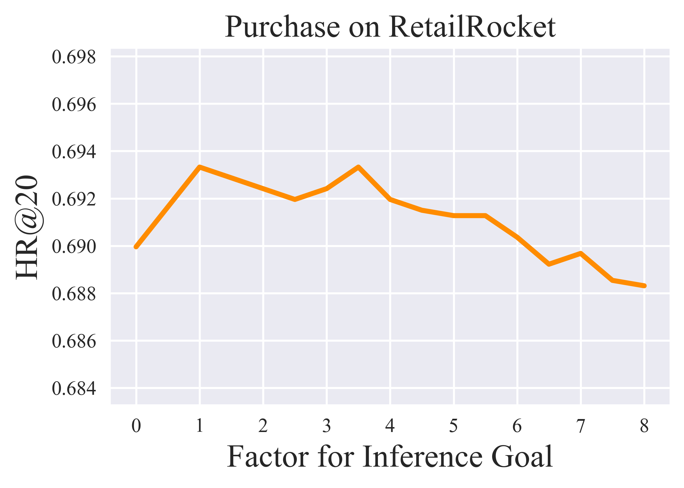
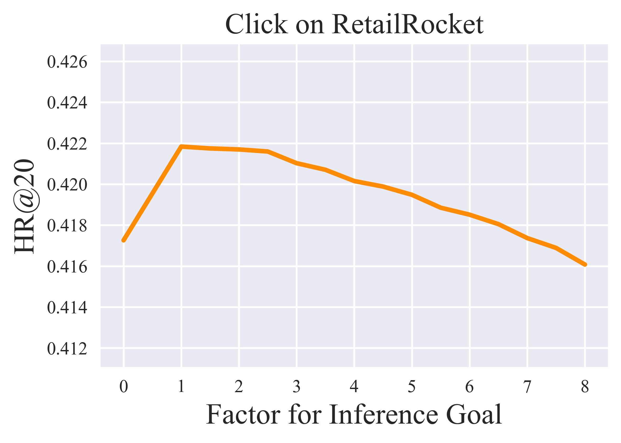
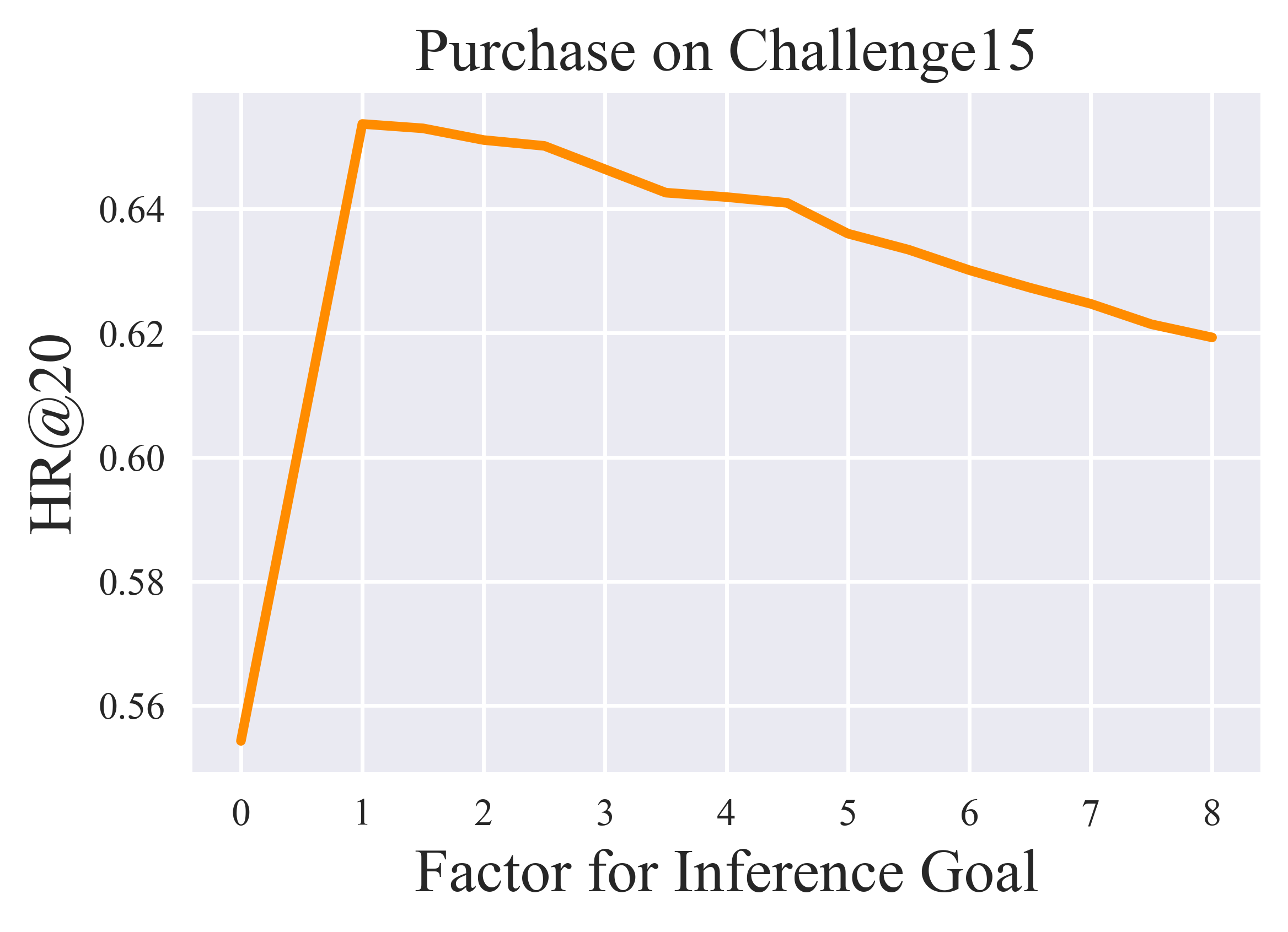
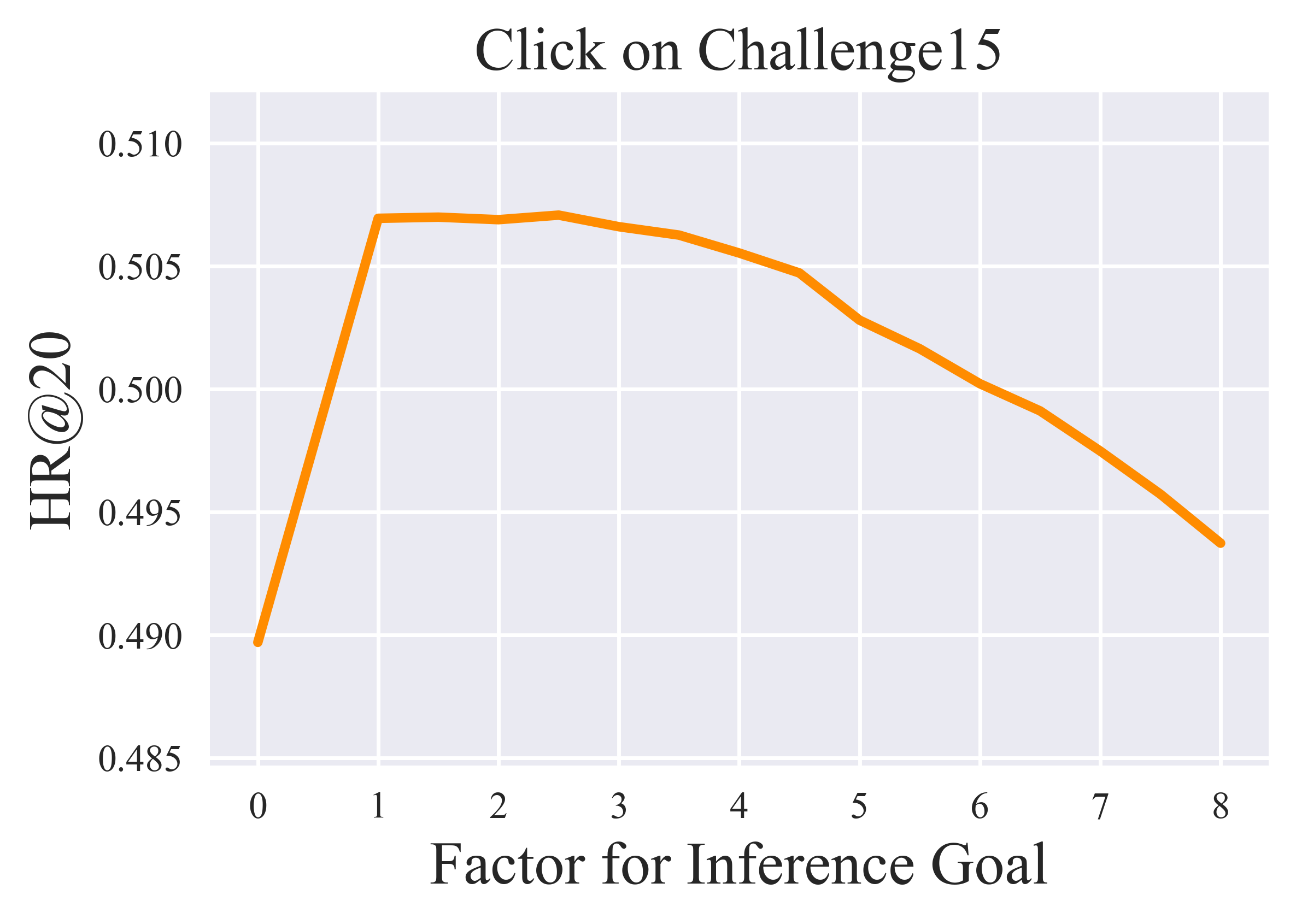
Figure 3: Performance of MOGCSL-S with different factors for inference goal.

References

- Ajay et al. (2020) Ajay, A.; Kumar, A.; Agrawal, P.; Levine, S.; and Nachum, O. 2020. Opal: Offline primitive discovery for accelerating offline reinforcement learning. arXiv preprint arXiv:2010.13611.
- Brandfonbrener et al. (2022) Brandfonbrener, D.; Bietti, A.; Buckman, J.; Laroche, R.; and Bruna, J. 2022. When does return-conditioned supervised learning work for offline reinforcement learning? Advances in Neural Information Processing Systems, 35: 1542–1553.
- Cai et al. (2022) Cai, Q.; Zhan, R.; Zhang, C.; Zheng, J.; Ding, G.; Gong, P.; Zheng, D.; and Jiang, P. 2022. Constrained reinforcement learning for short video recommendation. arXiv preprint arXiv:2205.13248.
- Chan et al. (2019) Chan, H.; Wu, Y.; Kiros, J.; Fidler, S.; and Ba, J. 2019. ACTRCE: Augmenting Experience via Teacher’s Advice For Multi-Goal Reinforcement Learning. arXiv preprint arXiv:1902.04546.
- Chane-Sane, Schmid, and Laptev (2021) Chane-Sane, E.; Schmid, C.; and Laptev, I. 2021. Goal-conditioned reinforcement learning with imagined subgoals. In International Conference on Machine Learning, 1430–1440. PMLR.
- Chen et al. (2021) Chen, L.; Lu, K.; Rajeswaran, A.; Lee, K.; Grover, A.; Laskin, M.; Abbeel, P.; Srinivas, A.; and Mordatch, I. 2021. Decision transformer: Reinforcement learning via sequence modeling. Advances in neural information processing systems, 34: 15084–15097.
- Chen and Guestrin (2016) Chen, T.; and Guestrin, C. 2016. Xgboost: A scalable tree boosting system. In Proceedings of the 22nd acm sigkdd international conference on knowledge discovery and data mining, 785–794.
- Emmons et al. (2021) Emmons, S.; Eysenbach, B.; Kostrikov, I.; and Levine, S. 2021. Rvs: What is essential for offline rl via supervised learning? arXiv preprint arXiv:2112.10751.
- Hidasi et al. (2015) Hidasi, B.; Karatzoglou, A.; Baltrunas, L.; and Tikk, D. 2015. Session-based recommendations with recurrent neural networks. arXiv preprint arXiv:1511.06939.
- Ho and Salimans (2022) Ho, J.; and Salimans, T. 2022. Classifier-free diffusion guidance. arXiv preprint arXiv:2207.12598.
- Kang and McAuley (2018) Kang, W.-C.; and McAuley, J. 2018. Self-attentive sequential recommendation. In 2018 IEEE international conference on data mining (ICDM), 197–206. IEEE.
- Li et al. (2023) Li, C.; Wang, Y.; Liu, Q.; Zhao, X.; Wang, W.; Wang, Y.; Zou, L.; Fan, W.; and Li, Q. 2023. STRec: Sparse transformer for sequential recommendations. In Proceedings of the 17th ACM Conference on Recommender Systems, 101–111.
- Lin et al. (2020) Lin, X.; Chen, H.; Pei, C.; Sun, F.; Xiao, X.; Sun, H.; Zhang, Y.; Ou, W.; and Jiang, P. 2020. A pareto-efficient algorithm for multiple objective optimization in e-commerce recommendation. In Proceedings of the 13th ACM Conference on recommender systems, 20–28.
- Liu, Zhu, and Zhang (2022) Liu, M.; Zhu, M.; and Zhang, W. 2022. Goal-conditioned reinforcement learning: Problems and solutions. arXiv preprint arXiv:2201.08299.
- Liu, Johns, and Davison (2019) Liu, S.; Johns, E.; and Davison, A. J. 2019. End-to-end multi-task learning with attention. In Proceedings of the IEEE/CVF conference on computer vision and pattern recognition, 1871–1880.
- Ma et al. (2018) Ma, J.; Zhao, Z.; Yi, X.; Chen, J.; Hong, L.; and Chi, E. H. 2018. Modeling task relationships in multi-task learning with multi-gate mixture-of-experts. In Proceedings of the 24th ACM SIGKDD international conference on knowledge discovery & data mining, 1930–1939.
- Mirza and Osindero (2014) Mirza, M.; and Osindero, S. 2014. Conditional generative adversarial nets. arXiv preprint arXiv:1411.1784.
- Misra et al. (2016) Misra, I.; Shrivastava, A.; Gupta, A.; and Hebert, M. 2016. Cross-stitch networks for multi-task learning. In Proceedings of the IEEE conference on computer vision and pattern recognition, 3994–4003.
- Roijers et al. (2013) Roijers, D. M.; Vamplew, P.; Whiteson, S.; and Dazeley, R. 2013. A survey of multi-objective sequential decision-making. Journal of Artificial Intelligence Research, 48: 67–113.
- Ruder (2017) Ruder, S. 2017. An overview of multi-task learning in deep neural networks. arXiv preprint arXiv:1706.05098.
- Sener and Koltun (2018) Sener, O.; and Koltun, V. 2018. Multi-task learning as multi-objective optimization. Advances in neural information processing systems, 31.
- Sohn, Lee, and Yan (2015) Sohn, K.; Lee, H.; and Yan, X. 2015. Learning structured output representation using deep conditional generative models. Advances in neural information processing systems, 28.
- Stamenkovic et al. (2022) Stamenkovic, D.; Karatzoglou, A.; Arapakis, I.; Xin, X.; and Katevas, K. 2022. Choosing the best of both worlds: Diverse and novel recommendations through multi-objective reinforcement learning. In Proceedings of the Fifteenth ACM International Conference on Web Search and Data Mining, 957–965.
- Wang et al. (2016) Wang, S.; Gong, M.; Li, H.; and Yang, J. 2016. Multi-objective optimization for long tail recommendation. Knowledge-Based Systems, 104: 145–155.
- Xin et al. (2020) Xin, X.; Karatzoglou, A.; Arapakis, I.; and Jose, J. M. 2020. Self-supervised reinforcement learning for recommender systems. In Proceedings of the 43rd International ACM SIGIR conference on research and development in Information Retrieval, 931–940.
- Xin et al. (2023) Xin, X.; Pimentel, T.; Karatzoglou, A.; Ren, P.; Christakopoulou, K.; and Ren, Z. 2023. Rethinking reinforcement learning for recommendation: A prompt perspective. In Proceedings of the 45th International ACM SIGIR Conference on Research and Development in Information Retrieval, 1347–1357.
- Yang et al. (2022) Yang, R.; Lu, Y.; Li, W.; Sun, H.; Fang, M.; Du, Y.; Li, X.; Han, L.; and Zhang, C. 2022. Rethinking goal-conditioned supervised learning and its connection to offline rl. arXiv preprint arXiv:2202.04478.
- Yu et al. (2020) Yu, T.; Kumar, S.; Gupta, A.; Levine, S.; Hausman, K.; and Finn, C. 2020. Gradient surgery for multi-task learning. Advances in Neural Information Processing Systems, 33: 5824–5836.
- Zhang and Yang (2021) Zhang, Y.; and Yang, Q. 2021. A survey on multi-task learning. IEEE Transactions on Knowledge and Data Engineering, 34(12): 5586–5609.
- Zheng, Zhang, and Grover (2022) Zheng, Q.; Zhang, A.; and Grover, A. 2022. Online decision transformer. In international conference on machine learning, 27042–27059. PMLR.