Continuous Gaussian Process Pre-Optimization for Asynchronous Event-Inertial Odometry

Abstract

Event cameras, as bio-inspired sensors, are asynchronously triggered with high-temporal resolution compared to intensity cameras. Recent work has focused on fusing the event measurements with inertial measurements to enable ego-motion estimation in high-speed and HDR environments. However, existing methods predominantly rely on IMU preintegration designed mainly for synchronous sensors and discrete-time frameworks. In this paper, we propose a continuous-time preintegration method based on the Temporal Gaussian Process (TGP) called GPO. Concretely, we model the preintegration as a time-indexed motion trajectory and leverage an efficient two-step optimization to initialize the precision preintegration pseudo-measurements. Our method realizes a linear and constant time cost for initialization and query, respectively. To further validate the proposal, we leverage the GPO to design an asynchronous event-inertial odometry and compare with other asynchronous fusion schemes within the same odometry system. Experiments conducted on both public and own-collected datasets demonstrate that the proposed GPO offers significant advantages in terms of precision and efficiency, outperforming existing approaches in handling asynchronous sensor fusion.

I Introduction

The estimation of ego-motion is critical for robots to accomplish automated tasks, including bridge inspection [1], disaster rescue [2], and autonomous driving [3]. Traditionally, this problem has been addressed by fusing various sensors using filter-based, optimization-based, or learning-based methods [4, 5, 6]. However, these conventional discrete-time estimation frameworks struggle with handling unsynchronized or high-frequency sensors effectively. To address this challenge, continuous-time methods have been proposed to associate measurements from different sensors with a unified, time-indexed trajectory, such as B-splines [7] or Temporal Gaussian Processes (TGP) [8].

Recent studies have demonstrated that event-inertial odometry based on continuous-time frameworks have great potential for ego-motion estimation in high-speed and High Dynamic Range (HDR) scenarios [9, 10]. Nonetheless, existing continuous-time event-inertial systems often involve a substantial number of inertial factors and optimize them together with kinematic states of motion trajectory, leading to high computational consumption. Other schemes integrate inertial measurements (referred to as preintegration) between keyframes to reduce the number of inertial factors, but paying the cost of neglecting the rich motion information between integration intervals. Consequently, event factors can only rely on an imprecise prior trajectory to build re-projection relationships. Since the prior trajectory may violate the true motion, it can corrupt the estimation.

Continuous-time preintegration methods mitigate these issues by modeling the integration procedure as continuous inference using differential equations or latent states [11, 12]. This enables the asynchronous fusion ability to query on a local inertial preintegration trajectory. The primary drawback is that the initialization and inference are still time-consuming for online applications. In addition. the differential equation-based methods often have less supports for asynchronous querying and back-end optimization.

To address these challenges, we propose a hybrid estimation framework that combines the advantages of both discrete- and continuous-time methods. We introduce a Temporal Gaussian Process (TGP)-based preintegration optimization, called GPO, to estimate the inertial pseudo-measurements. Our GPO employs a two-step optimization process to achieve linear solving and constant query times, enabling precise kinematic state queries at any time. Furthermore, we integrate GPO into an asynchronous event-inertial odometry system and demonstrate that our proposed approach outperforms state-of-the-art methods on both public and self-collected event-inertial datasets.

II Related Work

II-A Continuous-Time Estimation and Preintegration

The concept of preintegration was initially introduced by Lupton et al. [13]. On this basis, Forster et al. proposed preintegration on SO(3) manifold [14] which addresses the numerical singularity in attitude preintegration. Laterly, they successfully applied their method to a visual-inertial odometry [15]. In addition, Zhang et al. utilized the discrete-time preintegration to a TGP-based continuous-time multi-sensor fusion framework [16]. However, it can only offer a relative motion measurement between two adjacent motion states, and ignores the contribution of high-frequency motion information for asynchronous sensor fusion.

The discrete-time preintegration schemes assumes the constant measurements during each integration step, which may introduce high errors. To alleviate it, the differential equation-based preintegration methods were designed to model the rigid motion using the kinematic formula. For example, Shen et al. [17] first introduced a continuous form of preintegration, while Eckenhoff et al. [11] provided closed-form solutions for both preintegration and covariance propagation. The solid theoretical framework of this method was presented in [18], and they also incorporate their proposal into a graph-based sensor fusion system. Yang et al. [19] developed an efficient modularized formulation that accounts for bias states in the computation of inertial covariance. To further enable the asynchronous fusion, the Gaussian Process (GP)-based preintegration methods were proposed. The high-frequency preintegration is achieved by upsampling the raw IMU measurements and model the rotation integration as inference on the latent states of GP [20, 21]. But it only consider the 1-axis-rotation scenario and still rely on the iterative numerical integration. Further improvements were reported in LPM and GPM [22, 23] to continuously integrate on SO(3) using latent states of three independent GP. The LPM was subsequently involved in an event-inertial odometry systems [24]. Furthermore, they extended their proposal to support both attitude and translation preintegration in [12]. The latent states of six independent GP are solved with a least squares optimization problem, and endow an analytical preintegration ability using the linear operators. Although the latent state preintegration offers asynchronous fusion capabilities, its high computational burden can degenerate the real-time performance. Recently, Burnett et al. [25, 26] modeled the raw IMU measurements as the direct observations of the kinematic state of continuous-time trajectories, which can be employed in the TGP-based continuous-time framework. As mentioned in [9], this method has a low-precision in the asynchronous event-inertial odometry than the discrete-time and latent state schemes. In contrast, our proposal introduces the TGP theory into preintegration and suggests a two-step pre-optimization to initialize the preintegration. Combined with the concise propagation of Jacobians and covariances, our GPO achieves linear solving and constant querying time efficiency.

II-B Event-Inertial Odometry

Event-based visual-inertial odometry (EVIO) has garnered significant attentions for its potential to estimate ego-motion in challenging scenarios [27]. Zhu et al. [28] proposed a method to construct batch event packets aligned through two Expectation-Maximization steps [29], which were then fused with preintegrated IMU measurements in an Extended Kalman Filter (EKF) backend. Mahlknecht et al. [30] synchronized measurements from the Event-based KLT (EKLT) tracker [31] via extrapolation triggered by a fixed number of events, and then fused these visual measurements with IMU data in a filter-based backend. However, these methods suffer from high frontend computational complexity. Rebecq et al. [32] introduced a framework in which the corner features were detected on the motion-compensated event images, and tracked using Lucas-Kanade (LK) optical flow. Eventually, these tracked features were fused with discrete-time preintegration factors in a keyframe-based framework. This work was extended to Ultimate-SLAM [33] by incorporating intensity frames for enhancing robustness. Lee et al. [34] developed an 8-DOF warping model to fuse events and frames for accurate feature tracking, leveraging residuals from frontend optimization to update adaptive noise covariance.

Another trend involves utilizing the Time Surface (TS) [35], which stores the timestamp of the most recent event at each pixel, as a representation to enable frame-based detection and tracking techniques. Guan et al. [36] applied the Arc* [37] for corner detection and LK optical flow for tracking on polarity-encoded TS. They designed a tightly coupled graph-based optimization framework to fuse discrete-time preintegration results and event features. Based on this, PL-EVIO [38] integrated event-based line and point features with image-based point features, providing richer information in structured environments. For stereo configurations, Zhou et al. [39] proposed ESVO, the first event-based stereo visual odometry, which maximized spatiotemporal consistency using TS. Junkai et al. [40] extended this work to incorporate gyroscope measurements to mitigate degeneracy issues. Tang et al. [41] introduced an adaptive decay-based TS for feature extraction and proposed a polarity-aware strategy to enhance robustness. These tracked features were subsequently fused with discrete-time preintegration results using a Multi-State Constraint Kalman Filter (MSCKF). In general, these methods transform asynchronous event streams into synchronous data associations and convert high-rate IMU data into inter-frame motion constraints through discrete-time preintegration. However, the discrete-time estimation frameworks employed by existing event-inertial methods disrupt the asynchronous nature of event cameras, resulting in degraded performance in high-speed maneuvers.

To address this, several event-triggered inertial fusion frameworks have been proposed, preserving the high-temporal resolution and asynchronous properties of event cameras. Liu et al. [42] introduced a monocular asynchronous backend (without IMU), triggering optimization based on incoming events. Wang et al. [43] developed an event-based stereo VIO using TGP regression in an incremental backend. Dai et al. [24] proposed a tightly coupled event-inertial odometry framework based on inferring preintegration observations for each tracked event feature using LPM. Le et al. [44] extended this work by introducing a line feature tracker. Wang et al. [10] proposed a sliding-window TGP-based optimizer for asynchronous event odometry, and Li et al. [45] proposed to realize asynchronous fusion for event-inertial odometry using Gaussian Process Preintegration (GPP). Wang et al. [9] further extended this work by integrating various inertial fusion schemes and enabled the continuous-time estimation framework based on TGP.

III METHODOLOGY

III-A Inertial Preintegration

Define the measurements of the gyroscope and accelerometer be $\tilde{\bm{\omega}}_{m}$ and $\tilde{\bm{a}}$, respectively. We have the IMU’s measurement model as follows:

$$\tilde{\bm{\omega}}=\bm{\omega}_{b}^{bi}+\mathbf{b}_{g}+\bm{\varsigma}_{g},$$ (1)

$$\tilde{\bm{a}}=\bm{C}_{bi}(\ddot{\bm{r}}_{i}^{bi}-\bm{g}_{i})+\bm{b}_{a}+\bm{\varsigma}_{a},$$

where $\bm{\varsigma}_{g}\sim\mathcal{N}(\bm{0},\bm{Q}_{g})$ and $\bm{\varsigma}_{a}\sim\mathcal{N}(\bm{0},\bm{Q}_{a})$ are the measurement noises, $\bm{g}_{i}$ is the gravitational acceleration, and $\mathbf{b}_{g}$ and $\mathbf{b}_{a}$ are the gyroscope and accelerometer biases. According to the kinematic model of the rigid body, we have the integration formula as

$$\bm{C}_{k+1}=\bm{C}_{k}\prod_{t_{k}}^{t_{k+1}}\exp\left((\tilde{\bm{\omega}}(\tau)-\bm{b}_{g})d\tau\right),$$ (2)

$$\dot{\bm{r}}_{k+1}=\dot{\bm{r}}_{k}+\bm{g}_{i}\Delta t_{k}+\int_{t_{k}}^{t_{k+1}}\bm{C}(\tau)(\tilde{\bm{a}}(\tau)-\bm{b}_{a})d\tau,$$

$$\bm{r}_{k+1}=\bm{r}_{k}+\dot{\bm{r}}_{k}\Delta t+\frac{\bm{g}_{i}\Delta t^{2}_{k}}{2}+\int\!\!\!\int\bm{C}(\tau)(\tilde{\bm{a}}(\tau)-\bm{b}_{a})d\tau^{2},$$

where $\Delta t_{k}=t_{k+1}-t_{k}$, and $\bm{C}_{k},\dot{\bm{r}}_{k},\bm{r}_{k}$ are the rotation, linear velocity and translation of the rigid body at timestamp $t_{k}$. From (2), if the state variable $\bm{C}(\tau)$ updated during estimation, the integration needs be re-calculated again. To avoid the re-integration, $\bm{C}(\tau)$ is divided by $\bm{C}(\tau)=\bm{C}_{k}\bm{C}_{k}(\tau)$. The inertial preintegration measurements can be expressed by

$$\Delta\bm{C}=\prod_{t_{k}}^{t_{k+1}}\exp\left((\tilde{\bm{\omega}}(\tau)-\bm{b}_{g})d\tau\right),$$ (3)

$$\Delta\bm{v}=\int\bm{C}_{k}(\tau)(\tilde{\bm{a}}(\tau)-\bm{b}_{a})d\tau,$$

$$\Delta\bm{r}=\int\!\!\!\int\bm{C}_{k}(\tau)(\tilde{\bm{a}}(\tau)-\bm{b}_{a})d\tau^{2}.$$

Note that $\bm{C}_{k}(\tau)$ can be computed from $\Delta\bm{C}$ simultaneously. When the estimated IMU biases $\bm{b}_{a}$ and $\bm{b}_{g}$ are changed, the inertial preintegration measurements in (3) are updated with linearized Jacobians.

III-B GP Regression on Preintegration States

Although the inertial preintegration works well when applied in the discrete-time visual-inertial system, It would be suboptimal for the asynchronous measurement fusion, such as the event-inertial odometry and incompatible frequency measurements of gyroscopes and accelerometers. We address this drawback by integrating a pre-optimization step, where raw inertial measurements are modeled as a continuous-time trajectory using the sparse GP regression method.

Given the raw measurement $\tilde{\bm{\omega}}(\tau_{i})$ and $\tilde{\bm{a}}(\tau_{j})$, $\tau_{i},\tau_{j}\in[t_{k},t_{k+1}]$, we expect to search the preintegration pseudo-measurement at arbitrary timestamp $\tau\in[t_{k},t_{k+1}]$, even if the raw IMU measurements are asynchronous (i.e., $\tau_{i}\neq\tau_{j}$ when $i=j$ or $\tau_{i+1}-\tau_{i}\neq\tau_{i}-\tau_{i-1}$ or $\tau_{j+1}-\tau_{j}\neq\tau_{j}-\tau_{j-1}$). Assume the angular acceleration $\dot{\bm{\omega}}(\tau)$ to obey a zero-mean Gaussian process. The differential equation for the rotation preintegration state can be defined as

$$\dot{\bm{C}}(\tau)=\bm{C}(\tau)(\bm{\omega}(\tau))^{\land},\quad\dot{\bm{\omega}}(\tau)\sim\mathcal{GP}(\bm{0},\bm{Q}_{c}\delta(\tau-\tau^{\prime})),$$ (4)

where $\delta(\tau-\tau^{\prime})$ is the Dirac delta function and $\bm{Q}_{c}$ is the power spectral density matrix. Regard the rotation preintegration in (3) as a continuous-time process, we can leverage the Gaussian process in (4) to describe it, i.e.,

$$\bm{C}(\tau) =\mathbf{I}\quad\quad\quad\ \quad\text{if}\ \tau=t_{k},$$ (5)

$$\bm{C}(\tau) =\Delta\bm{C}\quad\quad\quad\text{if}\ \tau=t_{k+1},$$

$$\bm{\omega}(\tau) =\tilde{\bm{\omega}}(\tau)-\bm{b}_{g}.$$

where $\bm{\omega}(\tau)$ is modeled as the bias corrected angular velocity. A local variable $\bm{\phi}_{k}(\tau)$ is introduced to convert the nonlinear differential equation (4) to be a piece-wise linear one as

$$\bm{C}(\tau)=\bm{C}_{m}\exp((\bm{\phi}_{m}(\tau))^{\land}),$$ (6)

$$\ddot{\bm{\phi}}_{m}(\tau)\sim\mathcal{GP}(\bm{0},\bm{Q}_{c}\delta(\tau-\tau^{\prime})),$$

where $\bm{C}_{m}=\bm{C}(\tau_{m})$ is the linearization point. The time derivative of local variable has a relationship with the bias corrected angular velocity as $\bm{\omega}(\tau)=\bm{\mathcal{J}}(\bm{\phi}_{m}(\tau))\dot{\bm{\phi}}_{m}(\tau)$, where $\bm{\mathcal{J}}(\bm{\phi}_{m}(\tau))$ is the right Jacobian of $\bm{\phi}_{m}(\tau)$. In contrast, the state space equations for translation and velocity are inherently linear, defined as

$$\dot{\bm{r}}(\tau)=\bm{v}(\tau),\quad\dot{\bm{v}}(\tau)=\bm{a}(\tau),\quad\dot{\bm{a}}(\tau)\sim\mathcal{GP}(\bm{0},\bm{Q}_{r}\delta(\tau-\tau^{\prime})),$$ (7)

where $\bm{a}(\tau)=\bm{C}_{k}(\tau)(\tilde{\bm{a}}(\tau)-\bm{b}_{a})$ is a localized acceleration measurement corrected by the bias, and $\dot{\bm{a}}(\tau)$ is the “jerk” of the preintegration trajectory. In fact, both (6) and (7) has the similar closed-form solution as

$$\bm{x}_{m}(\tau) =\bm{\Lambda}_{m}(\tau)\bm{x}_{m}(\tau_{m})+\bm{\Psi}_{m}(\tau)\bm{x}_{m}(\tau_{m+1}),$$

$$\bm{\Lambda}_{m}(\tau) =\bm{\Phi}(\tau,\tau_{m})-\bm{\Psi}_{m}(\tau)\bm{\Phi}(\tau_{m+1},\tau_{m}),$$

$$\bm{\Psi}_{m}(\tau) =\bm{Q}_{m}(\tau)\bm{\Phi}(\tau_{m+1},\tau)^{\top}\bm{Q}_{m}(\tau_{m+1})^{-1},$$ (8)

where $\bm{x}_{m}(\tau)$ is the local state variable, $\bm{\Phi}(\tau,t_{m})$ is the transition function and $\bm{Q}_{m}(\tau)$ is the covariance matrix. In our context, the local state variables can be defined as $\bm{\gamma}_{m}(\tau)\doteq[\bm{\phi}_{m}(\tau),\dot{\bm{\phi}}_{m}(\tau)]$ for (6), and $\bm{p}_{m}(\tau)\doteq[\bm{r}(\tau),\bm{v}(\tau),\bm{a}(\tau)]$ for (7), respectively. In fact, $\bm{p}_{m}(\tau)=\bm{p}(\tau)$ is a global state variable, we add subscript $m$ for unifying the representation. As introduced in [45] and [46], the covariance matrices of two special sparse GP for (III-B) can be individually given by

$$\frac{\bm{Q}_{m}^{c}(\tau)=\begin{bmatrix}\frac{1}{3}\Delta\tau^{3}\bm{Q}_{c}&\frac{1}{2}\Delta\tau^{2}\bm{Q}_{c}\\ \frac{1}{2}\Delta\tau^{2}\bm{Q}_{c}&\Delta\tau\bm{Q}_{c}\end{bmatrix},}{\bm{Q}_{m}^{r}(\tau)=\begin{bmatrix}\frac{1}{20}\Delta\tau^{5}\bm{Q}_{r}&\frac{1}{8}\Delta\tau^{4}\bm{Q}_{r}&\frac{1}{6}\Delta\tau^{3}\bm{Q}_{r}\\ \frac{1}{8}\Delta\tau^{4}\bm{Q}_{r}&\frac{1}{3}\Delta\tau^{3}\bm{Q}_{r}&\frac{1}{2}\Delta\tau^{2}\bm{Q}_{r}\\ \frac{1}{6}\Delta\tau^{3}\bm{Q}_{r}&\frac{1}{2}\Delta\tau^{2}\bm{Q}_{r}&\Delta\tau\bm{Q}_{r}\end{bmatrix},}$$ (9)

where $\Delta\tau=\tau-\tau_{m}$, and $\bm{Q}_{c}$ and $\bm{Q}_{r}$ are generally set to be constant diagonal matrices. Their respective transition functions also have analytical expressions as

$$\frac{\bm{\Phi}^{c}(\tau,\tau_{m})=\begin{bmatrix}\mathbf{I}&\Delta\tau\mathbf{I}\\ \mathbf{0}&\mathbf{I}\end{bmatrix},}{\bm{\Phi}^{r}(\tau,\tau_{m})=\begin{bmatrix}\mathbf{I}&\Delta\tau\mathbf{I}&\frac{1}{2}\Delta\tau^{2}\mathbf{I}\\ \mathbf{0}&\mathbf{I}&\Delta\tau\mathbf{I}\\ \mathbf{0}&\mathbf{0}&\mathbf{I}\end{bmatrix}.}$$ (10)

III-C Two-steps Pre-Optimization

Let $\tau_{0}=t_{k}$ and $\tau_{M}=t_{k+1}$, we uniformly sample $M+1$ points within the preintegration period $[t_{k},t_{k+1}]$. By estimating GP states of these sampled timestamps, the raw IMU measurements within one preintegration period can be transfer to a continuous-time pseudo-measurement trajectory. Based on the foregoing pseudo measurement model, two pre-optimization steps are adopt to infer the pseudo-measurement trajectory. Let the global states for gyroscope preintegration be $\bm{\chi}_{m}^{g}=[\bm{C}_{m},\bm{\omega}_{m}]$, and for accelerometer preintegration be $\bm{\chi}_{m}^{a}=[\bm{r}_{m},\bm{v}_{m},\bm{a}_{m}]$, where $m\in{0,1,\cdots,M}$. The objective of pre-optimization, consisting of measurement residuals and GP prior residuals, can be defined as

$$\min_{\bm{\chi}_{m}^{g}}\sum_{i=0}^{N_{g}}\|\bm{e}_{g}^{m}(\tau_{i})\|^{2}_{Q_{g}}+\sum_{m=0}^{M}\|\bm{e}_{g}^{p}(\tau_{m})\|^{2}_{Q_{m}^{c}},$$ (11)

$$\min_{\bm{\chi}_{m}^{a}}\sum_{j=0}^{N_{a}}\|\bm{e}_{a}^{m}(\tau_{j})\|^{2}_{Q_{a}}+\sum_{m=0}^{M}\|\bm{e}_{a}^{p}(\tau_{m})\|^{2}_{Q_{m}^{r}},$$ (12)

where $\bm{e}_{g}^{m}$ and $\bm{e}_{a}^{m}$ indicates the gyroscope and accelerometer measurement residuals, and $\bm{e}^{p}_{g}$ and $\bm{e}^{p}_{a}$ are the corresponding GP prior residuals. We use different subscripts $\{i,j,m\}$ to represent the possible asynchronism among raw measurements and estimated pseudo preintegration states. Based on the prior assumptions in (6) and (7), the related prior residuals can be given by

$$\bm{e}_{g}^{p}(\tau_{m})=\left[\begin{array}[]{cc}\Delta\tau_{m}\bm{\omega}_{m}-\log(\bm{C}_{m}^{-1}\bm{C}_{m+1})\\ \bm{\omega}_{m}-\bm{\mathcal{J}}(\log(\bm{C}_{m}^{-1}\bm{C}_{m+1}))^{-1}\bm{\omega}_{m+1}\\ \end{array}\right],$$ (15)

$$\bm{e}_{a}^{p}(\tau_{m})=\left[\begin{array}[]{ccc}\Delta\tau_{m}\bm{v}_{m}+\frac{1}{2}\Delta\tau_{m}^{2}\bm{a}_{m}-\bm{r}_{m,m+1}\\ \bm{v}_{m}+\Delta\tau_{m}\bm{a}_{m}-\bm{v}_{m+1}\\ \bm{a}_{m}-\bm{a}_{m+1}\end{array}\right].$$ (19)

As we have regulated the analytical relationship between the GP state and the raw IMU measurement in (5) and (7), their corresponding residuals have concise forms as follows:

$$\bm{e}_{g}^{m}(\tau_{i}) =\tilde{\bm{\omega}}(\tau_{i})-\tilde{\bm{b}}_{g}-\bm{\omega}_{m}(\tau_{i}),$$ (20)

$$\bm{e}_{a}^{m}(\tau_{j}) =\bm{C}_{k}(\tau_{j})(\tilde{\bm{a}}(\tau_{j})-\tilde{\bm{b}}_{a})-\bm{a}_{m}(\tau_{j}).$$ (21)

Known that $\tau_{m}\leq\tau_{i}<\tau_{m+1}$, the $\bm{\omega}_{m}(\tau_{i})$ can be calculated by firstly interpolating the local state variable $\bm{\gamma}_{m}(\tau_{i})$ using (III-B) and then $\bm{\omega}_{m}(\tau_{i})=\bm{\mathcal{J}}(\bm{\phi}_{m}(\tau_{i}))\dot{\bm{\phi}}_{m}(\tau_{i})$. Similarly, the rotation component $\bm{C}_{k}(\tau_{j})$ can also be interpolated using (6) and (III-B). According to the prior model, the pseudo-acceleration $\bm{a}_{m}(\tau_{j})$ is directly assumed to be $\bm{a}_{m}$, if $\tau_{m}\leq\tau_{j}<\tau_{m+1}$.

III-D Event-Inertial Odometry

The proposed GP pre-optimization method is adopted to fuse the asynchronous event measurements coming from a monocular event camera. An asynchronous event-inertial odometry has been developed based on our previous work [9]. In our event-inertial odometry, the feature trajectories are tracked on the raw event streams using an event-driven frontend. These feature trajectories are inherently asynchronous with arbitrary sampling timestamps. Previous works usually leverage one continuous-time motion trajectory based on B-spline or GP regression to relate them with the inertial preintegration. Different from existing methods, we first adopt the proposed two-step GP pre-optimization to infer a series of local pseudo-measurement trajectories in a data-driven manner. Then, we fix the continuous-time local trajectory, and query the preintegration pseudo-measurements for asynchronous event projection factors. Subsequently, both the event and inertial observations are integrated into the backend factor graph. Eventually, the expected motion states are estimated by solving the factor graph with a sliding-window optimizer.

III-D1 Jacobians Derivation

For a given event projection factor occurring at an arbitrary timestamp, the residual Jacobians about neighbor estimated pose and velocity can be analytically inferred with the queried pseudo inertial integration. The Jacobians about estimated biases need further consideration. The previous GPP method calculates time-consuming numerical Jacobians of all latent states by extra integration steps. Instead, the proposed GPO memories the procedural Jacobians on timestamps of pseudo measurements using discrete-time formula and further propagates them to the arbitrary queried time using the Chain Rule. Assume $\bm{e}_{ev}(\tau)$ be an asynchronous event projection residual, the Jacobians can be derived by

$$\frac{\partial\bm{e}_{ev}(\tau)}{\partial\bm{b}(\tau)}=\frac{\partial\bm{e}_{ev}(\tau)}{\partial\bm{x}(\tau)}\left(\frac{\partial\bm{x}(\tau)}{\partial\bm{x}(\tau_{i})}\frac{\partial\bm{x}(\tau_{i})}{\partial\bm{b}(\tau)}+\frac{\partial\bm{x}(\tau)}{\partial\bm{x}(\tau_{i+1})}\frac{\partial\bm{x}(\tau_{i+1})}{\partial\bm{b}(\tau)}\right),$$ (22)

where $\tau\in[\tau_{i},\tau_{i+1}]$ is the projection timestamp, and $\bm{x}(\tau_{i})$ and $\bm{x}(\tau_{i+1})$ are two nearest neighbor pseudo states, and $\bm{b}(\tau)$ is the IMU bias variable. Normally, the Jacobian $\partial\bm{e}_{ev}(\tau)/\partial\bm{x}(\tau)$ can be derived from the observation model, and the Gaussian Process model of GPO can give $\frac{\partial\bm{x}(\tau)}{\partial\bm{x}(\tau_{i})}$ analytically. The pseudo state $\bm{x}(\tau_{i})$ is obtain by composing the last estimated state and later pseudo measurements, i.e., $\bm{x}(\tau_{i})=\bm{x}(t_{k})\boxplus\Delta\bm{x}(\tau_{i})$, where $\boxplus$ is the plus operator for linear vectors and the matrix multiply for Lie group. Note that $\Delta\bm{x}(\tau_{i})$ is first estimated by GPO, and then used as a pseudo measurement in the backend factor graph to estimate the system state $\bm{x}(t_{k})$. As done in previous work, the IMU bias is regard as constant within the whole integration period $[t_{k},t_{k+1})$. Therefore, we have

$$\frac{\partial\bm{x}(\tau_{i})}{\partial\bm{b}(\tau)}\approx\frac{\partial\bm{x}(\tau_{i})}{\partial\Delta\bm{x}(\tau_{i})}\frac{\partial\Delta\bm{x}(\tau_{i})}{\partial\bm{b}(\tau_{i})},$$ (23)

in which the procedural Jacobian $\frac{\partial\Delta\bm{x}(\tau_{i})}{\partial\bm{b}(\tau_{i})}$ can be efficiently inferred when initializing the pseudo measurements as done in discrete-time preintegration.

III-D2 Covariance Propagation

The asynchronous event factor can be integrated into the fusion problem by means of the proposed GPO method. Previous work normally consider a constant noise on all visual observations, which omits the effect of noisy pseudo inertial measurements and causes overconfidence on event observations. In this work, we derive the covariance propagation formula for the asynchronous event factor. In particular, the GPO memories the procedural covariance during its initialization, and then is used to interpolate the covariance at queried time. The interpolated covariance is propagated by the foregoing Jacobians to compute the process prior noise about event measurements. Eventually, the process prior noise is accumulated with the measurement noise of event camera.

$$\bm{\Sigma}_{\tau} =\lambda\bm{\Sigma}_{i}+(1-\lambda)\bm{\Sigma}_{i+1},$$

$$\bm{\Sigma}_{e} =\bm{J}\bm{\Sigma}_{\tau}\bm{J}^{\top}+\bm{\Sigma}_{s},$$ (24)

where $\lambda$ is the time-related weight coefficient from linear interpolation, and $\bm{\Sigma}_{s}\in\mathbb{R}^{2\times 2}$ is the sensor noise, and $\bm{J}$ is the stacked Jacobian of $\bm{e}_{ev}(\tau)$ w.r.t. $\bm{x}(\tau)$ and $\bm{b}(\tau)$. For high-frequency property of IMUs, the $\bm{\Sigma}_{\tau}$ can be approximated reasonably by linear interpolation. Intuitively, the projection factors queried far from system state $t_{k}$ will be assigned low confidence which is helpful for alleviating accumulative integration errors of IMU.

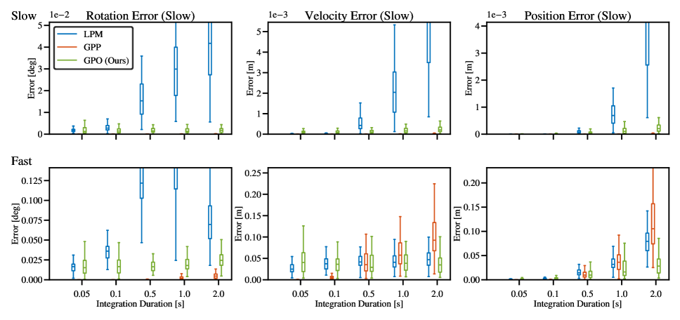
Figure 1: Precision comparison under various integration durations. The raw IMU measurements of two types of motions (Slow and Fast) are generated from simulation as done in [12]. For each integration period, we randomly select 100 trials, and compare their $\Delta\bm{C}$, $\Delta\bm{v}$, $\Delta\bm{r}$ with the ground truth. The GPP achieves the best precision for rotational integration in both slow and fast motions. The proposed GPO has higher precision than LPM in all situations and realizes the best performance for velocity and position integration of fast motions.

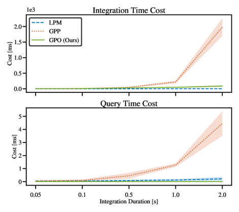
Figure 2: Time cost of integration and querying operations. The integration operation of the LPM acts like the discrete-time preintegration, and thus has the lowest time cost (top, blue dashed line). Although our GPO needs a two-step optimization, it is quite efficient and increases linearly with the number of integration time (top, green line). The GPP is the most time-consuming scheme (a cube time complexity, top, red dotted line), and its resolving time becomes unstable with the increasing integration duration (top, red shadow area). More importantly, our GPO accomplishes the best constant time cost for query pseudo measurements, Jacobians and covariance matrices (bottom, green line), which is ideal for fusing high-temporal resolution measurements of other asynchronous sensors.

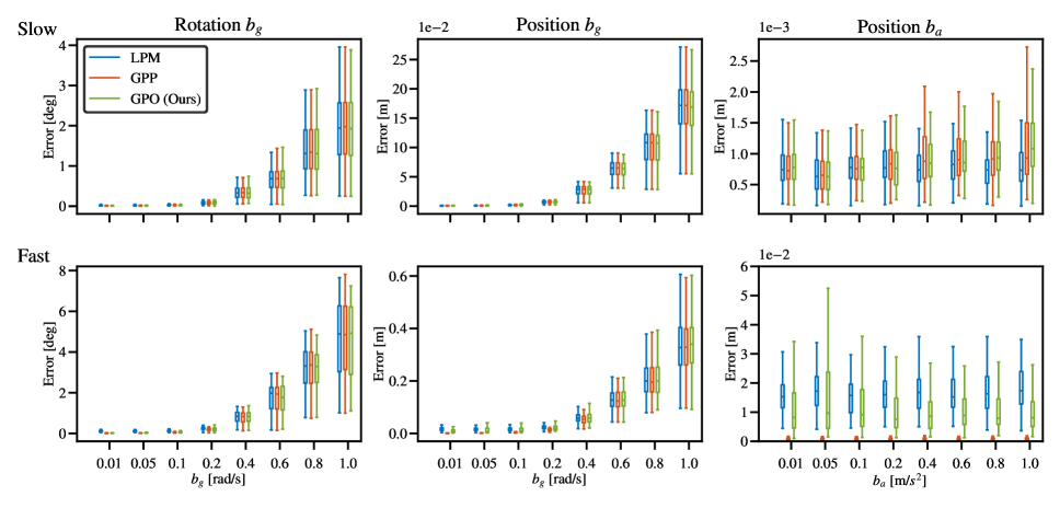
Figure 3: Procedual Jacobians evaluations. The Jacobian $\partial\Delta\bm{x}(\tau)/\partial\bm{b}(\tau)$ calculated using (22) and (23) is adopted to correct the integration results of known biases, and compared with the reintegration results. Ten interpolation time $\tau$ are randomly selected within the integration duration, and each evaluation is repeated with 100 trials. We show that the proposed approximate method (see Sec. III-D1) achieves competitive results in all cases.

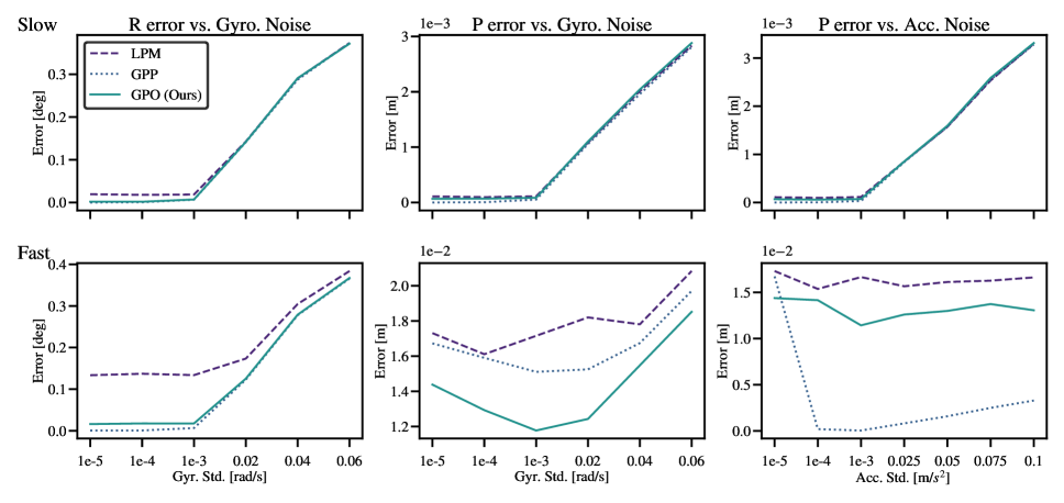
Figure 4: Robustness evaluations results. Varying degrees of Gaussian noises are mixed with raw IMU measurements (0.5 s, 100 Hz). All three methods performs similarly in slow motion with increasing noises. The proposed GPO has the best robustness in velocity integration and similar performances for attitude estimation with GPP.

IV Experiments

In the experiments, we compare the proposed GPO with two similar GP-based methods, LPM [23] and GPP [12], to evaluate their precision, robustness, and computational efficiency. Additionally, we develop an asynchronous event-inertial odometry system utilizing both GPO and GPP. Real-world experiments are then conducted to assess their performance when integrated into an asynchronous event-inertial fusion system.

IV-A Precision Comparison

We develop a IMU simulator according to [12] and generate raw IMU measurements and the ground truth with two various motion pattern, one for slow motion and one for fast motion. Then, we randomly integrate using LPM, GPP, and our GPO with five different integration periods and repeat each evaluation for 100 trials. For fairly comparing, we set the same Gaussian noise ($1\times 10^{-5}\ m/s^{2}$ for accelerometer and $1\times 10^{-5}\ rad/s$ for gyroscope ) and zero bias for all six axes. The errors of preintegration are shown in Fig. 1. We compare their $\Delta\bm{C}$, $\Delta\bm{v}$, $\Delta\bm{r}$ with the ground truth. The GPP achieves the best precision for rotational integration in both slow and fast motions. The proposed GPO has higher precision than LPM in all situations and realizes the best performance for velocity and position integration of fast motions.

IV-B Time-Complexity Comparison

We summary the time costs of preintegration and query, respectively. For each repeated integration period (100 trails), we randomly sample 10 times within the integration duration and call the query operation to compute the preintegration {$\Delta\bm{C}(\tau)$, $\Delta\bm{v}(\tau)$, $\Delta\bm{r}(\tau)$ } as well as the Jacobians and covariance. The results are displayed in Fig. 2. The integration operation of the LPM resembles discrete-time preintegration and demonstrates the lowest computational cost, as indicated by the blue dashed line in the top figure of Fig. 2. While our proposed GPO requires a two-step optimization process, it remains highly efficient, exhibiting a linear increase in computational cost with respect to the integration time, as shown by the green solid line in the top figure of Fig. 2. In contrast, the GPP is the most computationally expensive approach, characterized by a cubic time complexity (top, red dotted line in Fig. 2). Furthermore, its computation time becomes increasingly unstable as the integration duration grows, as illustrated by the red shaded area in the top figure of Fig. 2. Notably, our GPO achieves the best constant computational cost for querying pseudo-measurements, Jacobians, and covariance matrices, as depicted by the green solid line in the bottom figure of Fig. 2. This property makes GPO particularly well-suited for fusing high-temporal-resolution measurements from other asynchronous sensors.

IV-C Jacobians Evaluation

The Jacobians of preintgration results with respect ot IMU bias $\frac{\partial\Delta\bm{x}(\tau)}{\partial\bm{b}(\tau)}$ are calculated using (22) and (23). It is adopted to estimate IMU biases, and thereby correct the integration results in the fusion framework . Intuitively, The precision Jacobians would achieve better tightly-coupled fusion results. To evaluate it, we utilize the ground-truth biases and the Jacobians provided by different methods to correct the preintegration results and compared them with the reintegration known the biases. Ten interpolation time $\tau$ are randomly selected within the integration duration, and each evaluation is repeated with 100 trials. We show that the proposed approximate method (see Sec. III-D1) achieves competitive results in all cases.

IV-D Robustness against Noise

Inevitably, real IMU sensors contain varying degrees of noise. Therefore, robustness to noise is a crucial criterion for evaluating the performance of a preintegration method. To this end, we designed different noise levels in the simulator and calculated the preintegration errors under two motion patterns. The results are shown in Fig. 4. All three methods exhibit similar sensitivity to noise during slow motion. However, when applied to fast motion, GPO and GPP demonstrate superior noise robustness. Notably, under varying gyroscope noise levels, our GPO achieves lower positional integration errors compared to GPP, indicating enhanced robustness.

IV-E Experiments in Actual Event-Inertial Odometry

All three preintegration methods have been integrated into the same asynchronous event-inertial odometry system to ensure a fair comparison. In the frontend, our odometry system utilizes a fully asynchronous event feature tracker to obtain asynchronous observations. In the backend, these observations are then combined with continuous preintegration measurements, querying at the corresponding moments to form event re-projection factors. The overall integrated results are used as relative motion measurement factors between each pair of estimated system states. All these measurement factors are integrated into a factor graph, which is then optimized using a sliding window optimizer designed in our previous work. This approach leverages pre-optimization to reduce the computational burden before the backend optimization, resulting in more efficient and accurate estimation outcomes.

V Conclusion

In this study, we proposed a TGP-based preintegration method (GPO) and evaluated its performance against two similar GP-based methods, LPM and GPP. Our experimental results demonstrate that GPO effectively balances precision, robustness, and computational efficiency. Unlike LPM, which resembles discrete-time preintegration and incurs the lowest computational cost but lacks flexibility, GPO offers a linear time complexity with respect to integration duration while maintaining efficiency. In comparison to GPP, which suffers from cubic time complexity and instability during extended integration periods, GPO proves to be more reliable and robust. GPO achieves a constant computational cost for querying pseudo-measurements, Jacobians, and covariance matrices, making it particularly suitable for asynchronous sensor fusion tasks. Robustness analysis under varying noise levels reveals that GPO and GPP perform comparably under slow motion, but GPO outperforms both methods in fast-motion scenarios, achieving lower positional integration errors under gyroscope noise. We also present an event-inertial odometry with integrating all these preintegration schemes. Overall, the GPO method demonstrates significant potential for high-temporal-resolution applications, offering a robust and efficient solution for asynchronous fusion systems.

References

- [1] Z. Wang, X. Li, Y. Zhang, and P. Huang, “Localization, planning, and control of a uav for rapid complete coverage bridge inspection in large-scale intermittent gps environments,” IEEE Trans. Control Syst. Technol., pp. 1–13, 2024.
- [2] A. Albanese, V. Sciancalepore, and X. Costa-Pérez, “Sardo: An automated search-and-rescue drone-based solution for victims localization,” IEEE Transactions on Mobile Computing, vol. 21, no. 9, pp. 3312–3325, 2021.
- [3] H. Li, Y. Duan, X. Zhang, H. Liu, J. Ji, and Y. Zhang, “Occ-vo: Dense mapping via 3d occupancy-based visual odometry for autonomous driving,” in 2024 IEEE International Conference on Robotics and Automation (ICRA). IEEE, 2024, pp. 17 961–17 967.
- [4] A. Fornasier, P. van Goor, E. Allak, R. Mahony, and S. Weiss, “Msceqf: A multi state constraint equivariant filter for vision-aided inertial navigation,” IEEE Robotics and Automation Letters, vol. 9, no. 1, pp. 731–738, 2023.
- [5] X. Liu, S. Wen, Z. Jiang, W. Tian, T. Z. Qiu, and K. M. Othman, “A multi-sensor fusion with automatic vision-lidar calibration based on factor graph joint optimization for slam,” IEEE Transactions on Instrumentation and Measurement, 2023.
- [6] S. Klenk, M. Motzet, L. Koestler, and D. Cremers, “Deep event visual odometry,” in 2024 International Conference on 3D Vision (3DV). IEEE, 2024, pp. 739–749.
- [7] J. Lv, X. Lang, J. Xu, M. Wang, Y. Liu, and X. Zuo, “Continuous-time fixed-lag smoothing for lidar-inertial-camera slam,” IEEE/ASME Trans. Mechatronics, vol. 28, no. 4, pp. 2259–2270, 2023.
- [8] W. Talbot, J. Nubert, T. Tuna, C. Cadena, F. Dümbgen, J. Tordesillas, T. D. Barfoot, and M. Hutter, “Continuous-time state estimation methods in robotics: A survey,” arXiv preprint arXiv:2411.03951, 2024.
- [9] Z. Wang, X. Li, Y. Zhang, F. Zhang et al., “Asyneio: Asynchronous monocular event-inertial odometry using gaussian process regression,” arXiv preprint arXiv:2411.12175, 2024.
- [10] Z. Wang, X. Li, T. Liu, Y. Zhang, and P. Huang, “Asynevo: Asynchronous event-driven visual odometry for pure event streams,” arXiv preprint arXiv:2402.16398v2, 2024.
- [11] K. Eckenhoff, P. Geneva, and G. Huang, “High-accuracy preintegration for visual-inertial navigation,” in Algorithmic Foundations of Robotics XII: Proceedings of the Twelfth Workshop on the Algorithmic Foundations of Robotics. Springer, 2020, pp. 48–63.
- [12] C. Le Gentil and T. Vidal-Calleja, “Continuous latent state preintegration for inertial-aided systems,” Int. J. Robot. Res., vol. 42, no. 10, pp. 874–900, 2023.
- [13] T. Lupton and S. Sukkarieh, “Visual-inertial-aided navigation for high-dynamic motion in built environments without initial conditions,” IEEE Transactions on Robotics, vol. 28, no. 1, pp. 61–76, 2011.
- [14] C. Forster, L. Carlone, F. Dellaert, and D. Scaramuzza, “Imu preintegration on manifold for efficient visual-inertial maximum-a-posteriori estimation,” in Robotics: Science and Systems XI, 2015.
- [15] ——, “On-manifold preintegration for real-time visual–inertial odometry,” IEEE Trans. Robot., vol. 33, no. 1, pp. 1–21, 2016.
- [16] H. Zhang, C.-C. Chen, H. Vallery, and T. D. Barfoot, “Gnss/multi-sensor fusion using continuous-time factor graph optimization for robust localization,” IEEE Transactions on Robotics, 2024.
- [17] S. Shen, N. Michael, and V. Kumar, “Tightly-coupled monocular visual-inertial fusion for autonomous flight of rotorcraft mavs,” in 2015 IEEE International Conference on Robotics and Automation (ICRA). IEEE, 2015, pp. 5303–5310.
- [18] K. Eckenhoff, P. Geneva, and G. Huang, “Closed-form preintegration methods for graph-based visual–inertial navigation,” The International Journal of Robotics Research, vol. 38, no. 5, pp. 563–586, 2019.
- [19] Y. Yang, B. P. W. Babu, C. Chen, G. Huang, and L. Ren, “Analytic combined imu integration (aci 2) for visual inertial navigation,” in 2020 IEEE International Conference on Robotics and Automation (ICRA). IEEE, 2020, pp. 4680–4686.
- [20] C. Le Gentil, T. Vidal-Calleja, and S. Huang, “Gaussian process preintegration for inertial-aided state estimation,” IEEE Robot. Autom. Lett., vol. 5, no. 2, pp. 2108–2114, 2020.
- [21] ——, “3d lidar-imu calibration based on upsampled preintegrated measurements for motion distortion correction,” in 2018 IEEE International Conference on Robotics and Automation (ICRA). IEEE, 2018, pp. 2149–2155.
- [22] ——, “In2laama: Inertial lidar localization autocalibration and mapping,” IEEE Transactions on Robotics, vol. 37, no. 1, pp. 275–290, 2020.
- [23] C. Le Gentil and T. Vidal-Calleja, “Continuous integration over so (3) for imu preintegration,” Robot.: Sci. Syst., 2021.
- [24] B. Dai, C. Le Gentil, and T. Vidal-Calleja, “A tightly-coupled event-inertial odometry using exponential decay and linear preintegrated measurements,” in Proc. IEEE/RSJ Int. Conf. Intell. Robot. Syst. IEEE, 2022, pp. 9475–9482.
- [25] X. Zheng and J. Zhu, “Traj-lio: A resilient multi-lidar multi-imu state estimator through sparse gaussian process,” arXiv preprint arXiv:2402.09189, 2024.
- [26] K. Burnett, A. P. Schoellig, and T. D. Barfoot, “Continuous-time radar-inertial and lidar-inertial odometry using a gaussian process motion prior,” arXiv preprint arXiv:2402.06174, 2024.
- [27] G. Gallego, T. Delbrück, G. Orchard, C. Bartolozzi, B. Taba, A. Censi, S. Leutenegger, A. J. Davison, J. Conradt, K. Daniilidis et al., “Event-based vision: A survey,” IEEE Trans. Pattern Anal. Mach. Intell., vol. 44, no. 1, pp. 154–180, 2020.
- [28] A. Zihao Zhu, N. Atanasov, and K. Daniilidis, “Event-based visual inertial odometry,” in Proc. IEEE/CVF Conf. Comput. Vis. Pattern Recognit., 2017, pp. 5391–5399.
- [29] A. Z. Zhu, N. Atanasov, and K. Daniilidis, “Event-based feature tracking with probabilistic data association,” in Proc. IEEE Int. Conf. Robot. Autom. IEEE, 2017, pp. 4465–4470.
- [30] F. Mahlknecht, D. Gehrig, J. Nash, F. M. Rockenbauer, B. Morrell, J. Delaune, and D. Scaramuzza, “Exploring event camera-based odometry for planetary robots,” IEEE Robot. Autom. Lett., vol. 7, no. 4, pp. 8651–8658, 2022.
- [31] D. Gehrig, H. Rebecq, G. Gallego, and D. Scaramuzza, “Eklt: Asynchronous photometric feature tracking using events and frames,” Int. J. Comput. Vis., vol. 128, no. 3, pp. 601–618, 2020.
- [32] H. Rebecq, T. Horstschaefer, and D. Scaramuzza, “Real-time visual-inertial odometry for event cameras using keyframe-based nonlinear optimization,” in Proc. Brit. Mach. Vis. Conf., Sep. 2017, pp. 1–12.
- [33] A. R. Vidal, H. Rebecq, T. Horstschaefer, and D. Scaramuzza, “Ultimate slam? combining events, images, and imu for robust visual slam in hdr and high-speed scenarios,” IEEE Robot. Autom. Lett., vol. 3, no. 2, pp. 994–1001, 2018.
- [34] M. S. Lee, J. H. Jung, Y. J. Kim, and C. G. Park, “Event-and frame-based visual-inertial odometry with adaptive filtering based on 8-dof warping uncertainty,” IEEE Robot. Autom. Lett., 2023.
- [35] X. Lagorce, G. Orchard, F. Galluppi, B. E. Shi, and R. B. Benosman, “Hots: a hierarchy of event-based time-surfaces for pattern recognition,” IEEE Trans. Pattern Anal. Mach. Intell., vol. 39, no. 7, pp. 1346–1359, 2016.
- [36] W. Guan and P. Lu, “Monocular event visual inertial odometry based on event-corner using sliding windows graph-based optimization,” in Proc. IEEE/RSJ Int. Conf. Intell. Robot. Syst. IEEE, 2022, pp. 2438–2445.
- [37] I. Alzugaray and M. Chli, “Asynchronous corner detection and tracking for event cameras in real time,” IEEE Robot. Autom. Lett., vol. 3, no. 4, pp. 3177–3184, 2018.
- [38] W. Guan, P. Chen, Y. Xie, and P. Lu, “Pl-evio: Robust monocular event-based visual inertial odometry with point and line features,” IEEE Trans. Autom. Sci. Eng., pp. 1–17, 2023.
- [39] Y. Zhou, G. Gallego, and S. Shen, “Event-based stereo visual odometry,” IEEE Trans. Robot., vol. 37, no. 5, pp. 1433–1450, 2021.
- [40] J. Niu, S. Zhong, and Y. Zhou, “Imu-aided event-based stereo visual odometry,” arXiv preprint arXiv:2405.04071, 2024.
- [41] K. Tang, X. Lang, Y. Ma, Y. Huang, L. Li, Y. Liu, and J. Lv, “Monocular event-inertial odometry with adaptive decay-based time surface and polarity-aware tracking,” arXiv preprint arXiv:2409.13971, 2024.
- [42] D. Liu, A. Parra, Y. Latif, B. Chen, T.-J. Chin, and I. Reid, “Asynchronous optimisation for event-based visual odometry,” in Proc. IEEE Int. Conf. Robot. Autom., 2022, pp. 9432–9438.
- [43] J. Wang and J. D. Gammell, “Event-based stereo visual odometry with native temporal resolution via continuous-time gaussian process regression,” IEEE Robot. Autom. Lett., vol. 8, no. 10, pp. 6707–6714, 2023.
- [44] C. Le Gentil, F. Tschopp, I. Alzugaray, T. Vidal-Calleja, R. Siegwart, and J. Nieto, “Idol: A framework for imu-dvs odometry using lines,” in Proc. IEEE/RSJ Int. Conf. Intell. Robot. Syst. IEEE, 2020, pp. 5863–5870.
- [45] X. Li, Z. Wang, Y. Zhang, F. Zhang, and P. Huang, “Asynchronous event-inertial odometry using a unified gaussian process regression framework,” in Proc. IEEE/RSJ Int. Conf. Intell. Robot. Syst. IEEE, 2024, accepted.
- [46] T. Y. Tang, D. J. Yoon, and T. D. Barfoot, “A white-noise-on-jerk motion prior for continuous-time trajectory estimation on se(3),” IEEE Robot. Autom. Lett., vol. 4, no. 2, pp. 594–601, 2019.