Binary Evolution Pathways to Blue Large-Amplitude Pulsators: Insights from HD 133729

Blue Large-Amplitude Pulsators (BLAPs) represent a recently identified class of pulsating stars distinguished by their short pulsation periods (22–40 minutes) and asymmetric light curves. This study investigates the evolutionary channel of HD 133729, the first confirmed BLAP in a binary system. Through binary evolution simulations with MESA, we explored various mass ratios and initial orbital periods, finding that a mass ratio of q = 0.30 coupled with non-conservative mass transfer ($\rm\beta$= 0.15) successfully reproduces the observational characteristics(including luminosity, surface gravity, and effective temperature) of the binary system. Our models not only match the observed pulsational properties but also predict significant helium and nitrogen enhancements on the surface of the main-sequence companion. The system is expected to eventually undergo a common envelope phase leading to a stellar merger. Our findings provide crucial insights into the formation mechanism and evolutionary fate of BLAPs with main-sequence companions, while also placing constraints on the elemental abundances of their binary companions.

1 Introduction

Blue Large-Amplitude Pulsators (BLAPs) are a recently discovered class of pulsating stars, first observed by the Optical Gravitational Lensing Experiment (OGLE) survey in 2013 (e.g. Pietrukowicz et al. 2013). BLAPs are characterized by their short pulsation periods ranging from 22 to 40 minutes and their asymmetric light curves, which show a fast rise followed by a slower decline in brightness (e.g. Pietrukowicz et al. 2017). BLAPs lie on a region on the HR diagram between hot, massive main-sequence stars and hot subdwarfs. However, their luminosities ($\rm\log(L/L_{\odot})=2.2-2.6$) are about an order of magnitude higher than those of hot subdwarfs, while their surface gravities ($\rm\log(g/(cms^{-2}))=4.5-4.8$) are significantly lower. In addition to typical BLAPs, a class of high-gravity BLAPs also exists. While they have similar amplitudes to BLAPs, their spectroscopic properties and pulsation periods are more similar to those of sdB stars pulsating in the p-mode, with $\rm T_{eff}\simeq 32,000K$ and pulsation periods between 200 and 475 seconds (e.g. Kupfer et al. 2019). By combining photometric data from the Gaia and time-series data from the Zwicky Transient Facility(ZTF), McWhirter & Lam (2022) reported the discovery of 22 BLAP candidates, including six high-gravity pulsators. Notably, one object, designated ZGP-BLAP-01 (also known as TMTS-BLAP-1), with a pulsation period of 18.93 minutes, exhibits an unusually large period change rate of $2.2\times 10^{-6}\rm yr^{-1}$ (e.g. Lin et al. 2023).

The pulsation mechanism of BLAPs is attributed to the $\kappa$ mechanism, driven by the iron opacity bump at a specific temperature. The phenomenon of radiative levitation arises from the outward force exerted by stellar radiation on ions within a star. This phenomenon was originally proposed to explain the pulsations observed in hot subdwarf stars (e.g. Charpinet et al. 1996). Byrne & Jeffery (2018) highlighted the significant role of radiative levitation, which leads to the accumulation of iron and nickel around the temperature of $\simeq 2\times 10^{5}K$. This accumulation creates a substantial opacity bump to drive the pulsations observed in BLAPs.

In current research, numerous models have been proposed to explain the origin of BLAPs. These models are listed below:

(1) Low-Mass Pre-White Dwarf Model (pre-WDs)

BLAPs are interpreted as low-mass stars (typically 0.2-0.4$\rm M_{\sun}$) with helium cores. Their high effective temperatures and luminosities are sustained by residual hydrogen shell burning. These BLAPs primarily form through significant mass loss from a red giant star in binary systems, either through common envelope evolution or Roche lobe overflow (e.g. Romero et al. 2018; Byrne & Jeffery 2018; Córsico et al. 2018; Byrne et al. 2021).

(2) Helium-Burning Models

a) Core Helium-Burning Star Model

Wu & Li (2018) showed that core helium-burning stars evolved from initial masses $>4.0\rm M_{\sun}$ to final masses of 0.5-1.2$\rm M_{\sun}$ match observed BLAP properties, including effective temperature, luminosity, surface gravity, surface He/H ratio, pulsation periods, and period changes. In binary systems, Meng et al. (2020) demonstrated that using the common envelope wind (CEW) model, a surviving companion can evolve into a helium-burning star with a thin hydrogen envelope post-supernova, matching BLAP characteristics.

b) Shell Helium-Burning Star Model

BLAPs may be shell helium-burning subdwarf B-type (SHeB sdB) stars formed in long-period binary systems through stable RLOF. Studies of 304 binary evolution models show about half can produce SHeB sdBs matching observations, typically in systems with orbital periods $>1400$ days and main-sequence or white dwarf companions (e.g. Xiong et al. 2022).

(3) Stellar Merger Models

Different types of stellar mergers can form BLAPs. The merger of a helium white dwarf (HeWD) with a low-mass main-sequence (MS) star can form hot subdwarfs that evolve through BLAP-like states between helium shell ignition and core burning. (e.g., Zhang et al. 2023). The merger of double extremely low-mass (DELM) white dwarfs represents another promising formation channel for BLAPs. MESA modeling demonstrates that DELM WD mergers with total system masses between 0.32 and 0.7$\rm M_{\sun}$ can successfully produce BLAPs. After coalescence, these systems rapidly evolve into the BLAP phase within a few thousand years and maintain this state for 20,000-70,000 years before evolving further into hot subdwarfs. Eventually, they become either helium white dwarfs or hybrid He/CO white dwarfs. This formation scenario could explain the recent discovery of magnetic BLAPs since strong magnetic fields can be generated during the merger process (e.g. Kołaczek-Szymański et al. 2024). For clarity, I illustrate these models in Figure 1.

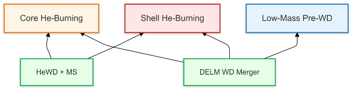
Figure 1: Schematic diagram of the origin of BLAPs. The stellar merger model can ultimately evolve into a pre-white dwarf, a core helium-burning star, or a shell-burning star. Arrows indicate the possible evolutionary paths to these states.

Although the total number of discovered BLAPs has exceeded 80, the number of confirmed BLAPs in binary systems remains limited(e.g. Pietrukowicz et al. 2024). TMTS-BLAP-1 potentially forms a wide binary with an orbital period of 1576 days (e.g. Lin et al. 2023). Recently, a detailed photometric analysis of HD 133729 based on TESS data revealed that this system consists of a late B-type main-sequence star and a BLAP companion, making it the first confirmed BLAP residing in a binary system (e.g. Pigulski et al. 2022).

The analysis of the TESS data from both sectors revealed a dominant frequency at $f_{P}=44.486d^{-1}$(pulsation period is the reciprocal of its frequency, i.e., 32.37 min) accompanied by its harmonics. The presence of the $f_{P}$ harmonics indicates a non-sinusoidal light curve, consistent with typical BLAP characteristics. Additionally, The light-travel-time effect (LTTE) manifests as orbital sidelobes in frequency spectra. These sidelobes appear at a frequency separation equal to the orbital frequency, $f_{orb}$. For HD 133729, the sidelobe separation of approximately $0.043d^{-1}$ implies an orbital period of $P_{orb}=f_{orb}^{-1}\approx 23$ days. Further observational data are presented in Table 1.

Table 1: Observational Data of HD 133729

	BLAP	B-type MS
L/$\rm L_{\sun}$	$2.15\pm 0.15$	$1.87\pm 0.12$
$\rm T_{eff}/K$	$11,500\pm 1000$	$29,000\pm 1800$
$\rm log(g/cm\,s^{-2})$	4.5	4.0
$\rm M/M_{\sun}$	-	$2.85\pm 0.25$

The formation and evolutionary path of the BLAP progenitor in HD 133729 can be potentially explained by two binary formation channels: the pre-WD RLOF/CE channel and the helium-burning RLOF/CE channel. Both scenarios require binary interaction. In the HD 133729 system, the B-type main-sequence star has a mass of $(2.85\pm 0.25)M_{\sun}$, implying that the initial star that formed the BLAP could only have been the primary.

If the BLAP was formed through the helium-burning star channel, its progenitor must also have undergone mass loss. Considering the minimum mass of a ZAMS that can evolve into a BLAP is 4 $\rm M_{\sun}$, it would need to lose 3.5 $\rm M_{\sun}$ to form a helium-burning star. Considering conservative mass transfer, the current B-type main-sequence star would have a mass larger than 3.5 $\rm M_{\sun}$(not matching the observed mass of the MS), making the helium core-burning star channel improbable.

Several open questions remain regarding the formation and evolutionary path of the BLAP in the HD 133729 system. Assuming the BLAP progenitor was the primary star, what specific channel led to its formation? Did it undergo Roche-lobe overflow (RLOF) or common envelope (CE) evolution through the pre-WD channel? Furthermore, what will the binary system’s subsequent evolution be after the BLAP crosses the pulsational instability strip? How do the surface abundances of B-type main-sequence stars in binary systems differ from those of single main-sequence stars? Such abundance anomalies, if present, can serve as valuable diagnostics for spectroscopic analyses.

While existing binary population synthesis models can identify potential pathways for stars to evolve into BLAPs, they cannot directly simulate the detailed binary evolution of this specific system. The HD 133729 system offers a unique opportunity to delve deeper into the formation and evolutionary mechanisms of BLAPs. This work aims to determine the evolutionary pathways and subsequent evolution of a class of BLAPs with main-sequence companions, analogous to the HD 133729 system.

The structure of this paper is as follows: In Section 2, we introduce the methods and parameter settings for stellar evolution and stellar pulsation calculations. Section 3 presents the evolutionary outcomes classified by different mass ratios. Section 4 comprises the discussion of the results. Finally, Section 5 summarizes the findings of this study.

2 Method

In order to investigate the origin of HD 133729, we use MESA (version r23.05.1) to simulate the evolution of binary systems (e.g. Paxton et al. 2011, 2013, 2015, 2018, 2019). The ”binary” module in MESA evolves binary systems by creating two single stars using the ”star” module. It can be used to evolve a primary star with a point-mass companion or to evolve both stars simultaneously. We co-evolve both stars simultaneously (e.g. Paxton et al. 2015).

First, we create a series of pre-main sequence stellar models using the create_pre_main_sequence_model in the ”star” module, as shown in Table 2. The metallicity chosen for our models is $Z=0.02$. For opacity, we selected the GS98 table (e.g. Grevesse & Sauval 1998). For the convection, we used the standard mixing length theory (MLT), with the parameter $\rm\alpha_{MLT}=2$. We have not included the effects of convective overshooting, thermohaline mixing, or semiconvection.

Then, we input primary and secondary into the ”binary” module. The mass transfer scheme uses the Ritter prescription (e.g. Ritter 1988). It assumes that matter flows through the inner Lagrangian point L1 as an isothermal, subsonic gas stream. This flow reaches the speed of sound as it approaches L1.

We considered both conservative and non-conservative evolution. In conservative evolution, the system undergoes mass transfer without additional rapid stellar wind mass loss. In non-conservative evolution, the system experiences mass loss during the mass transfer process. In MESA, it is assumed that the material lost through stellar winds carries the specific orbital angular momentum of its star. For cases with low mass transfer efficiency, the angular momentum loss follows the model by Soberman et al. (1997), where a fixed fraction of the transferred mass is lost either as fast isotropic stellar winds from each star or as a circumbinary matter ring with a certain radius. $\epsilon_{w}\equiv 1-\alpha-\beta$ represents the fraction of mass that is accreted. $\alpha$ is the fraction of mass directly lost as wind and $\beta$ is the fraction that is isotropically re-emitted. We explored different values of the $\beta$ to regulate the mass evolution of the main-sequence star, aiming to match the observed properties.

The calculation of the pulsation period used the formula:

$$M=\frac{10^{\langle\log(g)\rangle}R^{2}}{G}=\frac{10^{3\langle\log(g)\rangle}f^{4}}{G\omega^{4}}$$ (1)

This equation relates the mass (M) of the star to its surface gravity (g), radius (R), and pulsation frequency ($\omega$). The parameter $f=\omega/\omega_{dyn}$, where $\omega_{dyn}^{2}=GM/R^{3}$ is the dynamical frequency of the star. For low-mass helium-core pre-white dwarf models, $f\approx 3.6$. G is the gravitational constant (e.g. Kupfer et al. 2019). To compare the accuracy of formulas for calculating pulsation periods, we used GYRE to compute the l=0 radial pulsations of stellar evolutionary models. In the Eckart-Scuflaire-Osaki-Takata scheme, the meaning of $\rm n_{pg}$ is as follows:

$$n_{\mathrm{pg}}=\begin{cases}n_{\mathrm{p}}-n_{\mathrm{g}}&\text{for a }g_{n_{p}-n_{g}}\text{ mode}\\ n_{\mathrm{p}}-n_{\mathrm{g}}+1&\text{for a }p_{n_{p}-n_{g}+1}\text{ mode}\end{cases}$$ (2)

The pulsations of BLAPs are generally radial fundamental modes. Therefore, we only focus on the case where $\rm n_{pg}=1$ for p mode (e.g. Takata 2006).

Byrne et al. (2021) found no strong correlation between the initial and final masses of BLAPs, suggesting that binary parameters, such as the mass ratio and initial orbital period, are more significant factors in determining the final mass of BLAPs. Therefore, we performed binary evolution calculations for a range of binary mass ratios and initial orbital periods.

Table 2: Initial parameters of binary evolution

$q^{1}$	$\rm M_{1,i}(M_{\sun})$	$\rm M_{2,i}(M_{\sun})$	$\rm P_{\mathrm{min}}(day)^{2}$	$\rm P_{\mathrm{max}}(day)^{3}$	$\rm\Delta P(day)^{4}$	$\rm\beta^{5}$
	2.32	0.58	1.0	4.0	0.3	0
	2.40	0.60	1.0	4.0	0.3	0
0.25	2.48	0.62	1.0	4.0	0.3	0
	2.56	0.64	1.0	4.0	0.3	0
	2.64	0.66	1.0	4.0	0.3	0
	2.72	0.68	1.0	4.0	0.3	0
	2.23	0.67	1.0	4.0	0.3	0
	2.31	0.69	1.0	4.0	0.3	0
0.30	2.38	0.72	1.0	4.0	0.3	0
	2.46	0.74	1.0	4.0	0.3	0
	2.54	0.76	1.0	4.0	0.3	0
	2.62	0.78	1.0	4.0	0.3	0
	2.62	0.78	2.9	3.5	0.2	0.05
	2.62	0.78	2.9	3.5	0.2	0.10
0.30	2.62	0.78	2.9	3.5	0.2	0.15
	2.62	0.78	2.9	3.5	0.2	0.20
	2.14	0.75	1.0	4.0	0.3	0
	2.22	0.78	1.0	4.0	0.3	0
0.35	2.30	0.80	1.0	4.0	0.3	0
	2.37	0.83	1.0	4.0	0.3	0
	2.44	0.86	1.0	4.0	0.3	0
	2.52	0.88	1.0	4.0	0.3	0
	2.00	0.90	1.0	4.0	0.3	0
	2.07	0.93	1.0	4.0	0.3	0
0.45	2.14	0.96	1.0	4.0	0.3	0
	2.21	0.99	1.0	4.0	0.3	0
	2.28	1.02	1.0	4.0	0.3	0
	2.35	1.05	1.0	4.0	0.3	0

3 Result

We first rule out the CE channel. Using MESA calculations, with initial orbital periods longer than 100 days, the mass transfer rate rapidly exceeds $\rm 10^{-3}M_{\sun}\,yr^{-1}$ after the donor fills its Roche lobe, leading to CE evolution. We estimate that these systems will all merge, as the minimum $\rm\alpha_{CE}$ (common-envelope efficiency) required for envelope ejection exceeds 10. Therefore, we focus solely on RLOF.

3.1 Cases for $q=0.25$

For the case of q=0.25, we found that in models with an initial orbital period of 1.0 days, the primary star begins mass transfer while still in the main sequence stage, with a core hydrogen abundance of 0.17-0.21(depending on the masses of the binary components). At this time, the mass transfer timescale ($\rm\tau_{MT}\approx 10^{6.5}yr$) gradually decreases until it becomes smaller than the thermal timescale ($\rm\tau_{KH}\approx 10^{6}yr$). During this process, mass accretion can still be sustained. However, once the orbital period decreases to around 0.5 days, there is a sudden drop of the $\rm\tau_{MT}$($\approx 10^{4.2}yr$), further widening the discrepancy between $\rm\tau_{MT}$ and $\rm\tau_{KH}$ timescale. As shown in Figure 2(We have only chosen a set of cases with the highest binary masses as an illustration.), the mass transfer rate becomes too rapid (about $\rm 10^{-4}M_{\odot},yr^{-1}$), potentially leading to a common envelope phase. At this point, MESA is unable to continue the calculations, and the simulation stops.

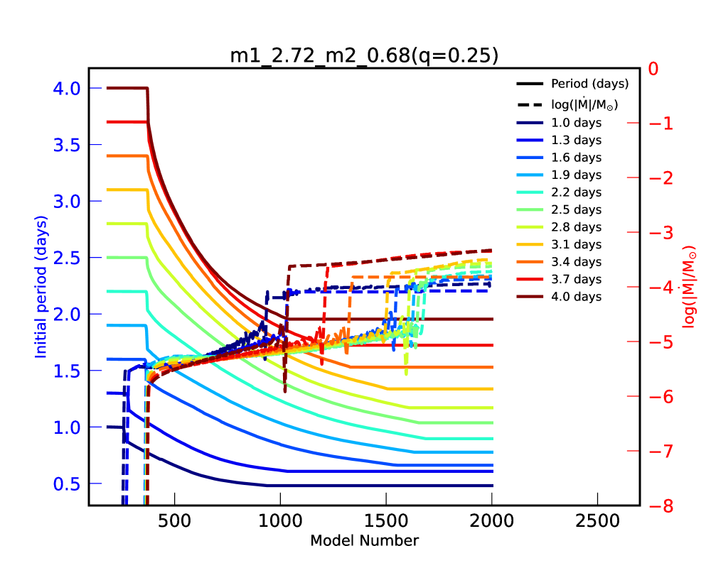
Figure 2: Period($\rm\dot{M}$)-model number diagram for a binary system with masses $\rm M_{1}=2.72M_{\sun}$ and $\rm M_{2}=0.68M_{\sun}$. The x-axis represents the model number. The left y-axis shows the orbital period in days, while the right y-axis displays the logarithm of the mass transfer rate. Colored lines represent different initial orbital periods ranging from 1.0 to 4.0 days. The solid and dashed lines represent the orbital period and the logarithm of the mass transfer rate, respectively.

A longer orbital period delays the onset of mass transfer, resulting in a lower hydrogen abundance in the primary star. However, similar to the case with an orbital period of 1.0 days, there is a sudden increase in the accretion rate when the orbital period shrinks to its minimum. This may indicate the system’s entry into a common envelope phase. As shown in Figure 1, even when the orbital period is increased to 4 days, the situation remains similar, with the accretion rate suddenly increasing to nearly $\rm 10^{-3}M_{\odot},yr^{-1}$. We speculate that in all cases with q=0.25, the sudden increase in the accretion rate after the orbital period shrinks to its minimum leading the system to enter a common envelope phase.

Therefore, with a mass ratio (q) of 0.25, the system cannot undergo stable mass transfer, thus excluding this scenario.

3.2 Cases for $q=0.35$

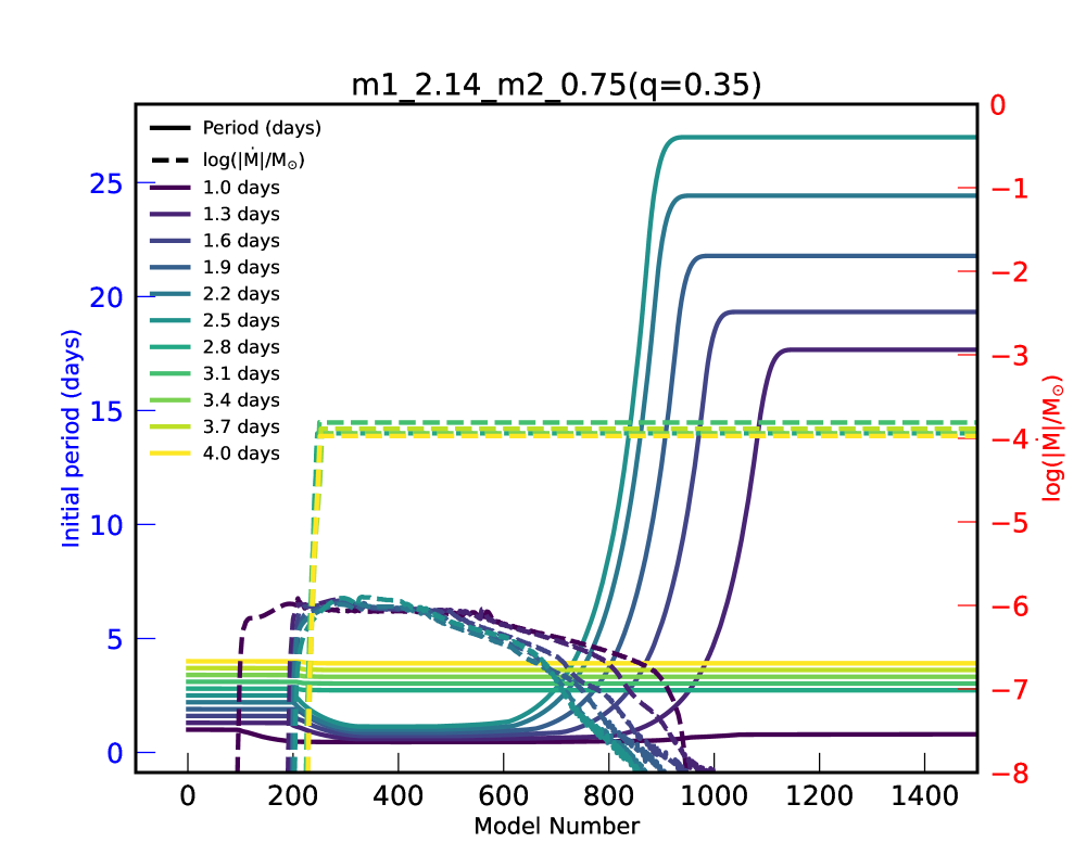
Figure 3: Period($\rm\dot{M}$)-model number diagram for a binary system with masses $\rm M_{1}=2.14M_{\sun}$ and $\rm M_{2}=0.75M_{\sun}$. The x-axis represents the model number. The left y-axis shows the initial orbital period in days, while the right y-axis displays the logarithm of the mass transfer rate. Colored lines represent different orbital periods ranging from 1.0 to 4.0 days. The solid and dashed lines represent the orbital period and the logarithm of the mass transfer rate, respectively.

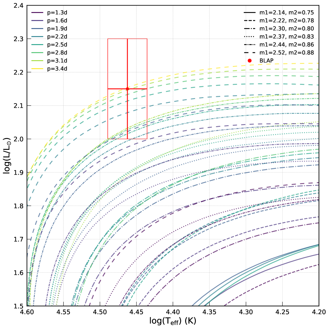
Figure 4: HR diagrams for all RLOF models with a mass ratio of 0.35. Different line styles represent different binary masses, and different colors represent different initial orbital periods.

In a model with a primary star of $\rm 2.14M_{\sun}$ and a secondary star of $0.75\rm M_{\sun}$, with an orbital period of 1 day, stable mass transfer can occur. The mass transfer rate remains consistently around $10^{-6}\,\rm M_{\sun}\,yr^{-1}$, until the primary star’s mass decreases to $0.73\rm M_{\sun}$ and the secondary star’s mass increases to $2.0\rm M_{\sun}$. At this point, the hydrogen in the core of the secondary star has been depleted. However, observations of BLAPS binaries show that the companion star is a main sequence star, indicating that this model does not meet the requirements. if the masses of both the primary and secondary stars are increased (even to their maximum values), the outcome remains similar: the secondary star evolves off the main sequence, yielding an analogous result to the previously described scenario.

The situation differs when the orbital period increases. As shown in Figure 3, for systems with a primary star mass of $\rm 2.14M_{\sun}$, a secondary star mass of $\rm 0.75M_{\sun}$, and an initial orbital period $\rm P_{i}(d)=1.3-2.5$, Roche Lobe Overflow (RLOF) commences when the primary star exhausts its core hydrogen and enters the Hertzsprung gap phase. After the mass transfer process concludes, the initial secondary star’s mass increases to $\rm 2.61-2.63M_{\sun}$, remaining a main-sequence star. If the initial orbital period $\rm P_{i}(d)=2.8-4.0$, the mass transfer rate reaches $\rm 10^{-3.8}M_{\sun}yr^{-1}$ from the outset. The mass transfer rate is very high, suggesting that the binary system likely enters a common envelope phase once mass transfer begins. Table 3 displays the evolutionary parameters of binary systems with q=0.35 that can undergo RLOF.

Figure 3 shows all cases where RLOF occurs at q=0.35, and the secondary star remains on the main sequence after the mass transfer process. It can be seen that only in the case with the highest initial mass ($\rm M_{1}=2.52M_{\sun}$ and $\rm M_{2}=0.88M_{\sun}$) and an initial orbital period between 2.2 and 3.4 days does the primary star’s evolutionary track cross the BLAP region. However, even when traversing the BLAP region, calculations reveal that the pulsation period remains below 32.37 minutes, which is inconsistent with observations. Therefore, we conclude that a mass ratio of q=0.35 cannot explain the observed BLAP binaries.

Table 3: Parameters for stable mass transfer models at q=0.35

$\rm M_{1,i}(M_{\sun})$	$\rm M_{2,i}(M_{\sun})$	$\rm P_{i}(day)^{1}$	$\rm M_{1,f}(M_{\sun})^{2}$	$\rm P_{f}(day)^{3}$
2.14	0.75	1.3-2.5	0.252-0.277	17.72-27.11
2.22	0.78	1.3-2.5	0.259-0.285	18.42-27.97
2.30	0.80	1.3-2.8	0.266-0.297	18.54-30.31
2.37	0.83	1.3-3.1	0.272-0.307	19.26-33.62
2.44	0.86	1.3-3.1	0.269-0.316	19.57-34.18
2.52	0.88	1.3-3.4	0.274-0.327	19.69-36.31

3.3 Cases for $q=0.45$

At this mass ratio, the binary evolution is similar to that with q=0.35. If the initial orbital period $\rm P_{i}=1.0day$ for all masses, the primary star initiates mass transfer during its main-sequence phase. The secondary accretes mass, which accelerates its evolution. Consequently, when the secondary exhausts its central hydrogen, the primary still retains approximately 0.03 solar masses of hydrogen. This is inconsistent with the observed evolutionary state of BLAP binaries, which consist of a pre-WD and a B-type main-sequence star.

If the initial orbital period of the binary is increased, the system can undergo RLOF mass transfer. For instance, with $\rm M_{1,i}=2.00M_{\sun}$ and $\rm M_{2,i}=0.90M_{\sun}$, at an initial orbital period $\rm P_{i}=1.3-2.2$ days, mass transfer begins after the primary star ends its main-sequence phase and enters the Hertzsprung gap, while the secondary star is still on the main sequence. After the mass transfer ends, the primary star has a mass of $0.265-0.282M_{\sun}$ and becomes the pre-WD, while the secondary star has a mass of $2.618-2.635M_{\sun}$ and remains a main-sequence star. However, after the mass transfer, the evolutionary track of the primary star on the HR diagram lies below the track of BLAPs, so a BLAP binary cannot be formed. At initial orbital periods of $\rm P_{i}=2.5-4.0days$, mass transfer still starts during the Hertzsprung gap phase, but the mass transfer rate rapidly increases to about $\rm 10^{-3.76}M_{\sun}yr^{-1}$, similar to what is shown in Figure 3, suggesting that the evolution has entered a common envelope phase. Increasing the binary mass yields similar results to those shown in Figure 4. Even in the case of maximum mass, the pulsation period of the BLAP cannot be matched with observations. All cases where RLOF occurs and the secondary remains a main-sequence star after mass transfer are listed in Table 4.

Table 4: Parameters for stable mass transfer at q=0.45

$\rm M_{1,i}(M_{\sun})$	$\rm M_{2,i}(M_{\sun})$	$\rm P_{i}(day)^{1}$	$\rm M_{1,f}(M_{\sun})^{2}$	$\rm P_{f}(day)^{3}$
2.00	0.90	1.3-2.2	0.265-0.282	21.24-31.30
2.07	0.93	1.3-2.2	0.262-0.283	24.18-33.97
2.14	0.96	1.3-2.5	0.263-0.288	26.20-40.56
2.21	0.99	1.3-2.8	0.264-0.294	28.35-46.82
2.28	1.02	1.3-2.8	0.262-0.299	27.52-48.27
2.35	1.05	1.3-3.1	0.265-0.309	28.76-53.21

3.4 Cases for $q=0.30$

3.4.1 From ZAMS to BLAP

Table 5: Parameters for stable mass transfer at q=0.30

$\rm M_{1,i}(M_{\sun})$	$\rm M_{2,i}(M_{\sun})$	$\rm P_{i}(day)^{1}$	$\rm M_{1,f}(M_{\sun})^{2}$	$\rm P_{f}(day)^{3}$
2.23	0.67	1.3-2.5	0.259-0.284	12.28-20.38
2.31	0.69	1.3-2.5	0.266-0.293	13.48-20.13
2.38	0.72	1.3-2.8	0.272-0.304	14.14-22.91
2.46	0.74	1.3-3.1	0.278-0.316	14.33-24.80
2.54	0.76	1.6-3.4	0.305-0.328	14.95-26.45
2.62	0.78	1.6-3.7	0.314-0.339	14.89-28.25

For models with an initial orbital period of 1 day, mass transfer begins before the primary star has exhausted its hydrogen. As mass transfer progresses, the orbital period decreases. When the orbital period reaches its minimum, the accretion rate suddenly jumps to approximately $\rm 10^{-4}M_{\sun}\,yr^{-1}$, similar to the q=0.25 case shown in Figure 2. This may indicate the onset of a common envelope phase. In the two sets of binary models with the largest initial masses (the last two sets of models shown in Table 5), which have an initial orbital period of 1.3 days, the evolution differs from those with q=0.35 and q=0.45, as no RLOF occurs. For these two mass sets, mass transfer begins before the primary star has exhausted its core hydrogen, with 0.04-0.06 of the core hydrogen remaining. When the orbital period reaches its minimum, the accretion rate also exhibits a sudden jump, increasing to approximately $\rm 10^{-3.9}M_{\sun},yr^{-1}$, possibly indicating the formation of a common envelope.

We focus on models with orbital periods longer than 1 day. Taking the binary system with the minimum mass as an example, where $\rm M_{1}=\rm 2.23M_{\sun}$ and $\rm M_{2}=\rm 0.67M_{\sun}$. Suppose the initial orbital period of the binary is between 1.3 and 2.5 days. In that case, the stars will exhaust the core hydrogen, enter the Hertzsprung gap phase, fill their Roche lobes, and initiate mass transfer via RLOF. The orbital period initially shortens, reaching a minimum, after which the masses of the primary and secondary stars reverse. Subsequently, the orbital period increases, and the radius of the primary star shrinks significantly, no longer filling its Roche lobe, thus ending the mass transfer. The mass of $\rm M_{1}$ becomes $\rm 0.259-0.284M_{\sun}$, the mass of $\rm M_{2}$ becomes $\rm 2.616-2.641M_{\sun}$ , and the orbital period becomes 12.28-20.38 days. The post-mass transfer parameters for more massive binaries are listed in Table 5. Models with orbital periods outside the range for RLOF likely entered a common envelope phase because the mass transfer rate was too high when mass transfer began. This is similar to the case shown in Figure 3.

We have identified a set of models capable of undergoing RLOF. However, these models still lack accurate matching with the observed final orbital period and pulsation period. Therefore, we further refine the RLOF models. The observed orbital period of the BLAP object is 23.08 days. To find the best-matching models, we plotted the initial and final orbital periods for the last four sets of models (see Table 5), as shown in Figure 5. We can use a polynomial fit to determine the best-fit orbital period. We identified four models whose final orbital periods are very close to 23.08 days. We then plotted the HR diagram for these binary systems, as shown in Figure 6. We found that models with $\rm M_{1}$ masses of $\rm 2.46M_{\sun}$, $\rm 2.54M_{\sun}$, and $\rm 2.62M_{\sun}$ all pass through the BLAP region. However, the effective temperatures of the main sequence stars are higher than the observed value. We will address this issue in the next section.

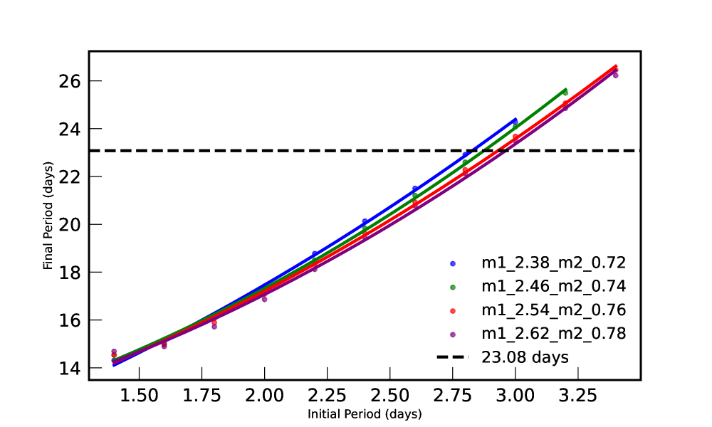
Figure 5: Plot of the final orbital period against the initial orbital period for the four highest binary masses with a mass ratio of 0.30. Polynomial fits are applied to the four datasets. The horizontal dashed black line represents a final orbital period of 23.08 days.

Figure 6: Panel (a) shows the HR diagram for the primary star in four models. The initial periods used for the four models are the optimal periods determined from polynomial fits. Panel (b) shows the HR diagram for the secondary star in the four models.

As shown in Figure 7, two models ($\rm M_{1}$ with $\rm 2.54M_{\sun}$ and $\rm 2.62M_{\sun}$, respectively) fall within the $\rm logT_{eff}$ range of BLAPs and pass through the appropriate log(g). However, only the $\rm M_{1}$ with $\rm 2.62M_{\sun}$ crosses the 32.37-minute pulsation period within the $\rm logT_{eff}$ region of BLAPs. We also need to compare the relative rate of period change. The observed relative rate of period change is $\rm r\equiv\dot{P}_{P}/P_{P}=(-11.5\pm 0.6)\times 10^{-7}\,yr^{-1}$. We can calculate the relative rate of period change at a pulsation period of 32.37 minutes, and the result is $\rm r\equiv\dot{P}_{P}/P_{P}=-1.9\times 10^{-6}\,yr^{-1}$. The difference between these two values lies within one order of magnitude.

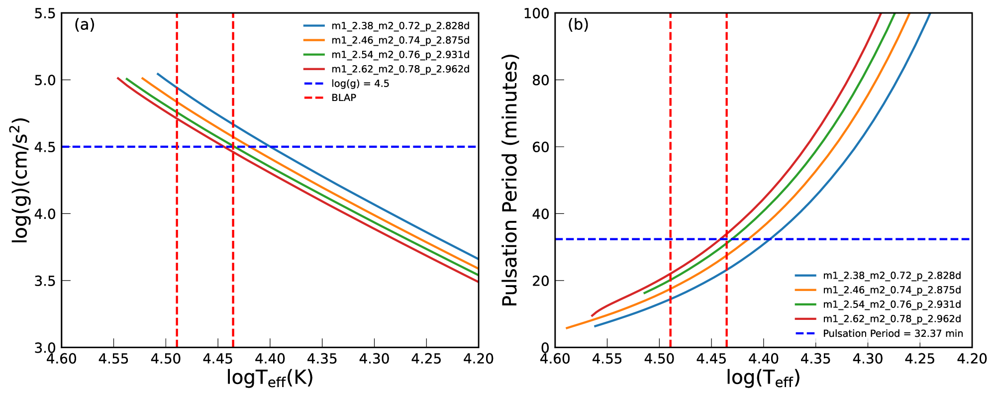
Figure 7: Panel (a) shows the $\rm logT_{eff}$ vs. log(g) diagram for the four models. The red dashed line represents the $\rm logT_{eff}$ range for the BLAPs, and the dark blue dashed line indicates a log(g) of 4.5. Panel (b) shows the $\rm logT_{eff}$ vs. pulsation period diagram. The red dashed line again represents the $\rm logT_{eff}$ range for BLAPs, while the dark blue dashed line represents a pulsation period of 32.27 minutes.

This model can explain the observed BLAPs for the following reasons: 1. The primary star can evolve through the region of the HR diagram corresponding to the BLAP region. 2. While traversing this region, the pulsation period can reach 32.27 minutes. 3. During its evolution across the HR diagram, the primary star can also pass through a log(g)=4.5. 4. At a pulsation period of 32.27 minutes, the relative rate of period change is $\rm-1.9\times 10^{-6}\,yr^{-1}$. Although this does not perfectly match the observed value, it is within the same order of magnitude.

3.4.2 Consider the $\beta$ value in the mass transfer processes.

Because the $\rm logT_{eff}$ of the B-type main-sequence star in the previous model calculation was about 1400K higher than the observed value (Figure 6), we speculated that the mass transfer process should be non-conservative rather than conservative. This speculation is reasonable and allows us to define

$$\beta^{\star}=-\frac{\dot{M}_{a}}{\dot{M}_{d}}=\min\left(\frac{CM_{a}/\tau_{KH,a}}{M_{d}/\tau_{KH,d}},1\right)$$ (3)

where $\rm\tau_{KH}$ is the Kelvin-Helmholtz timescale, $\rm\dot{M}_{d}$ is the mass-loss rate of the donor star, $\rm\dot{M}_{a}$ is the mass-accretion rate onto the accretor, and C accounts for the increase in the maximum accretion rate due to the expansion of the accreting star (e.g. Paczyński & Sienkiewicz 1972; Neo et al. 1977; Hurley et al. 2002; Schneider et al. 2015). During Case A mass transfer, if the component stars have roughly comparable masses, then $\rm\beta^{\star}\approx 1$. During Case B/C mass transfer - when the donor star is more evolved – $\rm\beta^{\star}$ is typically closer to 0. It is evident that the mass transfer in our model is Case B, and $\rm\beta^{\star}$ can be different from 1 (note that the definition of $\rm\beta^{\star}$ here is the opposite of that in MESA).

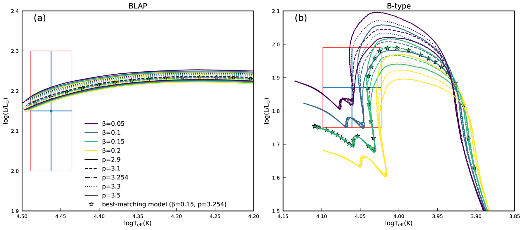
Figure 8: Panel (a) shows the HR diagram for the primary star, taking into account the parameter $\rm\beta$. Different colors represent different $\rm\beta$ values, and different line styles represent different initial orbital periods. The pentagram highlights the best-match model with a final orbital period closest to 23.08 days. Panel (b) shows the HR diagram for the secondary star, also considering the $\rm\beta$ parameter, with the same color and line style conventions as Panel (a).

We performed calculations considering $\rm\beta$. We chose the $\rm M_{1}=2.62M_{\sun}$ $\rm M_{2}=0.78M_{\sun}$, with an initial period of 2.9-3.5 days and a time step of 0.2 days. We also chose different $\rm\beta$ values: 0.05, 0.10, 0.15, and 0.20. Following the method of finding the best final period in the q=0.30 subsection, we also found the best-matching model to be $\rm P_{i}=3.254$ day. As shown in Figure 8, the evolutionary results indicate that the position of the B-type main-sequence star on the HR diagram is closely related to the $\rm\beta$ value. The larger the $\rm\beta$ value, the lower the luminosity and effective temperature of the main-sequence star. We found that when $\rm\beta$ is 0.15, the difference between the effective temperature and the observed value is only about 300K, and the luminosity is also within the error range. Considering the non-conservative mass transfer scenario can better explain the observational results of the B-type main-sequence star. We calculated the time for the binary system to evolve from the main sequence to the BLAP stage, and the time spent in the BLAP region, to be $\rm 4.44\times 10^{8}yr$ and $\rm 2.19\times 10^{5}yr$, respectively.

4 Disscusion

4.1 Post-BLAP Evolution

After the binary system passed through the BLAP phase(here is the best matching model for Figure 8), we continued to evolve it. Now, the B-type main-sequence star has become the donor, and the BLAP has become the accretor. When the donor evolves to the tip of the red giant branch, it expands to fill its Roche lobe and transfers mass to its companion. Currently, the mass ratio(q) is as small as 0.12, making stable mass transfer unlikely($\rm\dot{M}\approx 10^{-3}M_{\sun}\,yr^{-1}$). We speculate that the system has entered the common envelope phase. Following the BLAP phase, the system takes $\rm 5.5\times 10^{8}yr$ to reach the CE phase. We show the HR diagram of the post-BLAP stage in Figure 9.

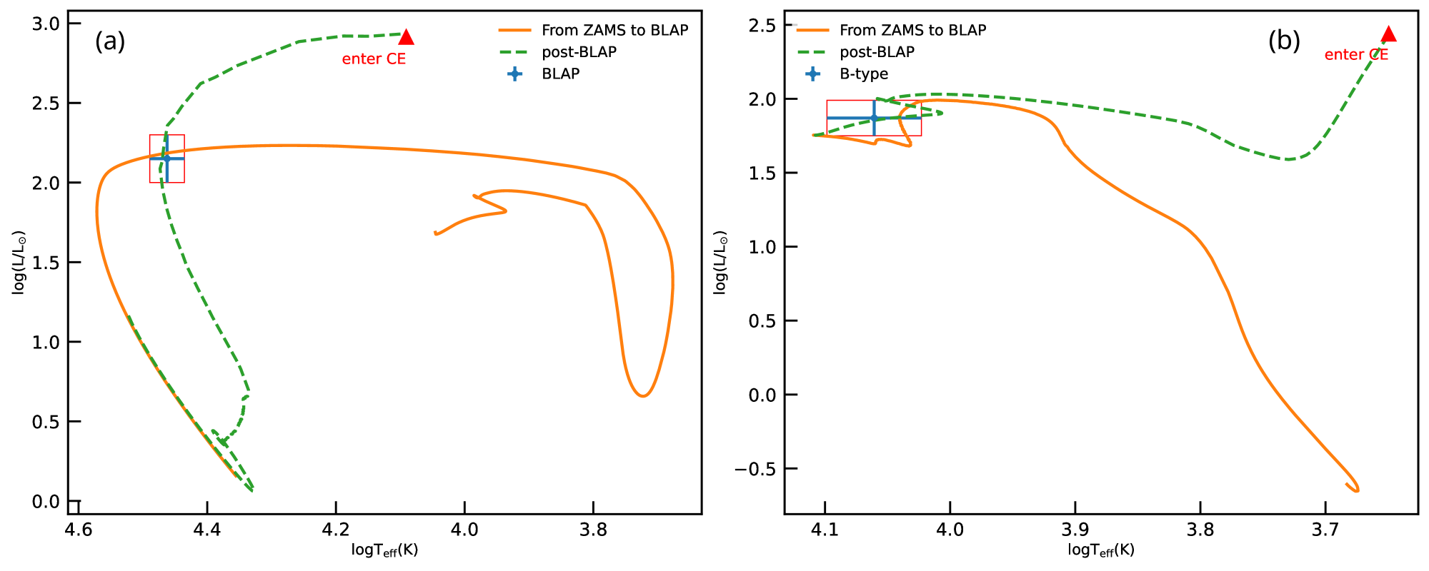
Figure 9: Panel (a) and Panel (b) show the HR diagrams of BLAP and B-type main sequence stars under the best-fitting model in Figure 7. The orange solid line represents the evolutionary track from the ZAMS to the BLAP region, while the green dashed line depicts the evolutionary track from the BLAP phase to the onset of the CE phase. The red triangle indicates the point where the system enters the CE phase.

We calculated the binding energy of the main-sequence star to be $\rm-5.43\times 10^{48}erg$. Assuming an extreme case of common envelope ejection, the limiting separation of the two stars is $\rm R_{1,core}+R_{2}=0.294R_{\sun}$, while the separation before entering the common envelope phase is $a=49R_{\sun}$. Thus, the orbital energy is reduced by $\rm 7.61\times 10^{47}erg$. Using these two energy values, the calculated $\rm\alpha_{CE}$ is approximately 7.14. The widely used range of $\rm\alpha_{CE}$ is about 0-1.5. This implies that it is highly unlikely for the orbital energy to be sufficient to expel the envelope, and we conclude that the two stars will eventually merge.

4.2 Elemental Abundances on the Surfaces of MS

In binary systems, particularly those undergoing mass transfer, the accretion of material from a donor star onto its companion can significantly alter the surface abundances of the accreting star. For instance, helium enrichment often serves as a direct indicator of mass accretion from a helium-rich donor. Similarly, enhancements in nitrogen relative to carbon and oxygen can signal the accretion of CNO-processed material. These elemental signatures are instrumental in diagnosing the history of mass transfer and the evolutionary pathways that have led to the current state of the binary system.

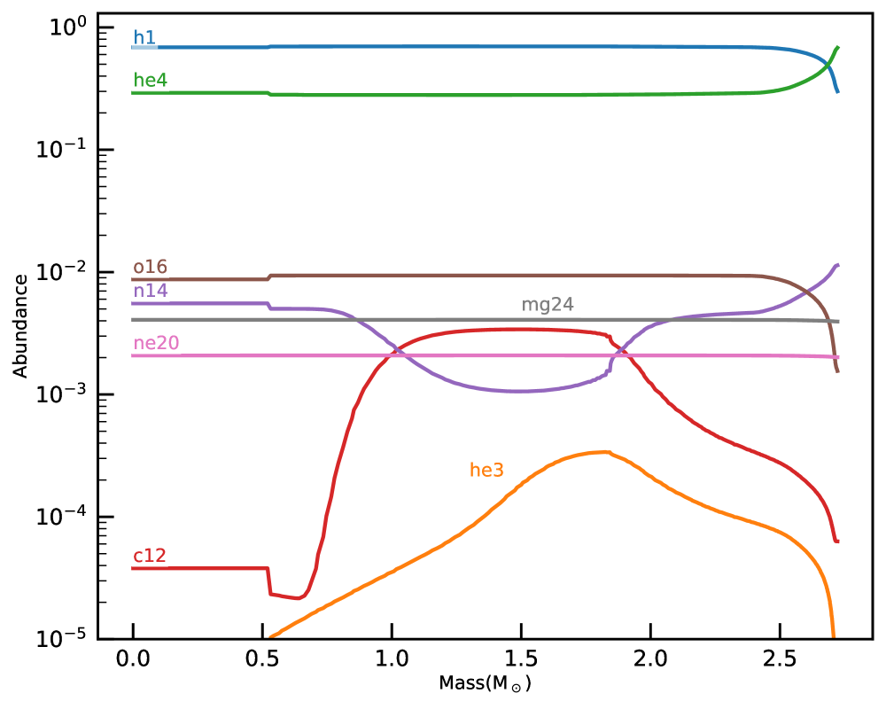
Figure 10: The elemental abundance distributions in the main-sequence companion star following the mass transfer. The solid lines in different colors represent various elements and can find the significant enrichment of $\rm{}^{4}He$ (green) and $\rm{}^{14}N$ (purple) in particular.

Our MESA simulations provide theoretical predictions for the surface elemental abundances of the B-type MS companion in the HD 133729 system. As depicted in Figure 10, the simulations indicate significant enhancements in both He and N on the surface of the accreting MS star. Specifically, the surface He abundance reaches values as high as 0.68, and the N abundance increases to 0.01, both of which are substantially higher than those typically observed in normal MS stars. These elevated abundances are consistent with the accretion of CNO-processed material from a previously evolved donor star.

However, the lack of detailed spectroscopic analysis for HD 133729 presents a challenge for directly validating our theoretical models. Future high-resolution spectroscopic studies are crucial for accurately measuring the surface abundances of He and N in the B-type companion. Confirming these abundance anomalies would strengthen the rationality of this evolutionary pathway.

4.3 Adiabatic calculation of GYRE

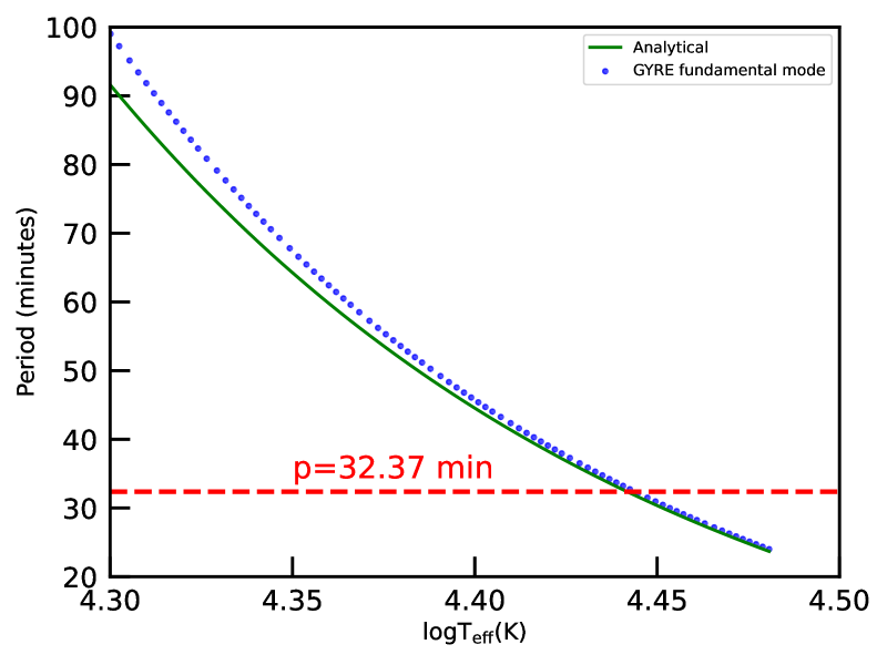
Figure 11: The $\rm logT_{eff}$ vs. pulsation period diagram for the best-match model shown in Figure 8. The green solid line represents the results calculated using Equation 1, while the blue dotted line shows the results of adiabatic pulsation calculations using GYRE.

Kupfer et al. (2019) used formula (1) to calculate the pulsation period of high-gravity BLAPs. We aim to validate this formula for normal BLAPs. We calculated the fundamental mode pulsation periods of BLAPs near 32.75 minutes using adiabatic mode computations with GYRE, as shown in Figure 11. Around 32.75 minutes, the formula provides an excellent match to the GYRE computations, further demonstrating the efficacy of this formula for a wide range of BLAPs.

4.4 Pulsational instability uncertainties

While we can calculate pulsation periods using analytical formulae or numerical tools like GYRE, this does not guarantee that stars are pulsationally unstable as they evolve through these regions. Our calculations have not incorporated pulsational instability analysis under nonadiabatic conditions.

Byrne & Jeffery (2020) investigated the pulsational stability of pre-WD models during their evolution. They first performed adiabatic analyses to identify the eigenfrequencies of the stars. These adiabatic results were then used as initial guess values for nonadiabatic analyses to determine the stability of the identified modes. They found that the radial fundamental mode is unstable from an effective temperature of roughly 30,000K to at least 50,000K, and possibly even as high as 80,000K. In this temperature range, the periods of the unstable fundamental mode vary from around 100 seconds to as long as 2-3 hours.

Romero et al. (2018) also found unstable modes for three harmonic degrees. g modes with l = 1 and l = 2 are unstable for radial orders in the range $29\leq k\leq 39$ and $54\leq k\leq 67$, respectively. The radial fundamental mode is also unstable, suggesting that the modes observed in BLAPs with periods of 1200-1500 seconds could be radial modes. The observed periods in BLAP stars can be explained by non-radial g modes with high radial order or, alternatively, by low-order radial modes in the case of the shortest periods.

4.5 MESA-RSP

The MESA-RSP (Radial Stellar Pulsations) software package, integrated into MESA, has become a powerful tool for studying stellar pulsations. This package can reliably simulate large-amplitude, self-excited, nonlinear pulsations in classical pulsating stars, making it particularly valuable for studying BLAPs. Jadlovský et al. (2024) pioneered the first comprehensive exploration of BLAP theoretical instability regions using MESA-RSP, constructing an extensive grid of models with masses ranging from $\rm 0.3-1.1M_{\sun}$, luminosities spanning $\rm log(L/L_{\sun})=1.5-3.5$, and effective temperatures between 20-35 kK. Their analysis revealed that for lower luminosities ($\rm\sim 200L_{\sun}$), as observed by Pigulski et al. (2022) and Bradshaw et al. (2024), the fundamental mode periods of lower-mass models ($\rm 0.3-0.4M_{\sun}$) show better agreement with observations and empirical relations, particularly the period-luminosity relation.

4.6 Broader applications of the model

Figure 9 of Byrne et al. (2021) presents the orbital period and companion mass distribution for stars in the BLAP evolutionary phase. The orbital period exhibits a bimodal distribution, with a minor peak around 1.2 days and a more prominent peak at an orbital period of $10^{1.6}$ days ($\sim$40 days). Based on the orbital period of HD 133729 and our model calculations, we propose that the second peak in the orbital period distribution likely arises from RLOF, while the first peak originates from the CE ejection. Our aim is not only to explain HD 133729, but also to provide a broad grid of calculated parameters. We anticipate that our non-conservative mass transfer RLOF models will be applicable to newly discovered BLAP binary systems with main-sequence companions.

5 Summary

This study systematically investigates the origin and evolution of binary BLAP systems consisting of a BLAP and a main sequence star, with particular emphasis on explaining the origin of the HD 133725 system. Using MESA stellar evolution code, we performed comprehensive binary evolution simulations exploring a range of mass ratios (q = 0.25, 0.30, 0.35, 0.45) and initial orbital periods to identify viable progenitor channels. Our detailed parameter space exploration strongly supports the pre-white dwarf RLOF channel as the formation pathway for HD 133729.

Under conservative mass transfer, a mass ratio of q = 0.30 can reasonably reproduce the observed orbital period, pulsation period, and rate of period change. However, the effective temperature of the B-type main-sequence star is overestimated in this scenario. Considering non-conservative mass transfer with an isotropic re-emission wind efficiency of $\rm\beta$ = 0.15 yields a better match to the observed effective temperature. The best-fit binary model for the system has component masses of $\rm M_{1,i}=2.68M_{\sun}$ and $\rm M_{2,i}=0.78M_{\sun}$, and $\rm P_{i}=3.254\,day$. We expect the system to undergo a common envelope phase during the second mass transfer episode, ultimately leading to a merger.

The evolution of surface abundances provides an important test of our models. Following the first mass transfer phase, we predict significant surface abundance anomalies in the B-type main-sequence companion, including enhanced helium and nitrogen. These predictions arise from the accretion of CNO-processed material and provide testable diagnostics for future high-resolution spectroscopic observations.

This comprehensive study explains the specific case of HD 133729 and provides a theoretical framework for understanding similar BLAP binary systems. Our findings suggest that non-conservative RLOF is likely a common formation channel for BLAPs with main-sequence companions, particularly for systems with orbital periods around 20-30 days. The surface abundance predictions we have made offer a clear path for observational tests of our model through future high-resolution spectroscopic studies. Such observations will be crucial for further constraining the evolutionary pathways of the BLAP binary and validating our theoretical understanding of their formation and evolution.

6 Acknowledgments

This study is supported by the National Natural Science Foundation of China (Nos 12225304, 12288102, 12090040/12090043, 12473032), the National Key R&D Program of China (No. 2021YFA1600404), the Western Light Project of CAS (No. XBZG-ZDSYS-202117), the science research grant from the China Manned Space Project (No. CMS-CSST-2021-A12), the Yunnan Revitalization Talent Support Program (Yunling Scholar Project), the Yunnan Fundamental Research Project (No 202201BC070003), and the International Centre of Supernovae, Yunnan Key Laboratory (No. 202302AN360001).

References

- Bradshaw et al. (2024) Bradshaw, C. W., Dorsch, M., Kupfer, T., et al. 2024, MNRAS, 527, 10239
- Byrne & Jeffery (2018) Byrne, C. M. & Jeffery, C. S. 2018, MNRAS, 481, 3810
- Byrne & Jeffery (2020) Byrne, C. M. & Jeffery, C. S. 2020, MNRAS, 492, 232
- Byrne et al. (2021) Byrne, C. M., Stanway, E. R., & Eldridge, J. J. 2021, MNRAS, 507, 621
- Charpinet et al. (1996) Charpinet, S., Fontaine, G., Brassard, P., & Dorman, B. 1996, ApJ, 471, L103
- Córsico et al. (2018) Córsico, A. H., Romero, A. D., Althaus, L. G., Pelisoli, I., & Kepler, S. O. 2018, arXiv e-prints, arXiv:1809.07451
- Grevesse & Sauval (1998) Grevesse, N. & Sauval, A. J. 1998, Space Sci. Rev., 85, 161
- Hurley et al. (2002) Hurley, J. R., Tout, C. A., & Pols, O. R. 2002, MNRAS, 329, 897
- Jadlovský et al. (2024) Jadlovský, D., Das, S., & Molnár, L. 2024, arXiv e-prints, arXiv:2408.16912
- Kołaczek-Szymański et al. (2024) Kołaczek-Szymański, P. A., Pigulski, A., & Łojko, P. 2024, A&A, 691, A103
- Kupfer et al. (2019) Kupfer, T., Bauer, E. B., Burdge, K. B., et al. 2019, ApJ, 878, L35
- Lin et al. (2023) Lin, J., Wu, C., Wang, X., et al. 2023, Nature Astronomy, 7, 223
- McWhirter & Lam (2022) McWhirter, P. R. & Lam, M. C. 2022, MNRAS, 511, 4971
- Meng et al. (2020) Meng, X.-C., Han, Z.-W., Podsiadlowski, P., & Li, J. 2020, ApJ, 903, 100
- Neo et al. (1977) Neo, S., Miyaji, S., Nomoto, K., & Sugimoto, D. 1977, PASJ, 29, 249
- Paczyński & Sienkiewicz (1972) Paczyński, B. & Sienkiewicz, R. 1972, Acta Astron., 22, 73
- Paxton et al. (2011) Paxton, B., Bildsten, L., Dotter, A., et al. 2011, ApJS, 192, 3
- Paxton et al. (2013) Paxton, B., Cantiello, M., Arras, P., et al. 2013, ApJS, 208, 4
- Paxton et al. (2015) Paxton, B., Marchant, P., Schwab, J., et al. 2015, ApJS, 220, 15
- Paxton et al. (2018) Paxton, B., Schwab, J., Bauer, E. B., et al. 2018, ApJS, 234, 34
- Paxton et al. (2019) Paxton, B., Smolec, R., Schwab, J., et al. 2019, ApJS, 243, 10
- Pietrukowicz et al. (2017) Pietrukowicz, P., Dziembowski, W. A., Latour, M., et al. 2017, Nature Astronomy, 1, 0166
- Pietrukowicz et al. (2013) Pietrukowicz, P., Dziembowski, W. A., Mróz, P., et al. 2013, Acta Astron., 63, 379
- Pietrukowicz et al. (2024) Pietrukowicz, P., Latour, M., Soszynski, I., et al. 2024, arXiv e-prints, arXiv:2404.16089
- Pigulski et al. (2022) Pigulski, A., Kotysz, K., & Kołaczek-Szymański, P. A. 2022, A&A, 663, A62
- Ritter (1988) Ritter, H. 1988, A&A, 202, 93
- Romero et al. (2018) Romero, A. D., Córsico, A. H., Althaus, L. G., Pelisoli, I., & Kepler, S. O. 2018, MNRAS, 477, L30
- Schneider et al. (2015) Schneider, F. R. N., Izzard, R. G., Langer, N., & de Mink, S. E. 2015, ApJ, 805, 20
- Soberman et al. (1997) Soberman, G. E., Phinney, E. S., & van den Heuvel, E. P. J. 1997, A&A, 327, 620
- Takata (2006) Takata, M. 2006, PASJ, 58, 893
- Wu & Li (2018) Wu, T. & Li, Y. 2018, MNRAS, 478, 3871
- Xiong et al. (2022) Xiong, H., Casagrande, L., Chen, X., et al. 2022, A&A, 668, A112
- Zhang et al. (2023) Zhang, X., Jeffery, C. S., Su, J., & Bi, S. 2023, ApJ, 959, 24