Chiral phase transition: effective field theory and holography

Abstract

We consider chiral phase transition relevant for QCD matter at finite temperature but vanishing baryon density. Presumably, the chiral phase transition is of second order for two-flavor QCD in the chiral limit. Near the transition temperature, we apply the Schwinger-Keldysh formalism and construct a low energy effective field theory (EFT) for the system, in which fluctuations and dissipations are systematically captured. Dynamical variables involve chiral charge densities and order parameter. The EFT action is further confirmed within a modified AdS/QCD model using the holographic Schwinger-Keldysh technique. With suitable higher terms neglected, the stochastic equations derived from the EFT resemble those of model F in the Hohenberg-Halperin classification. Within the EFT, we briefly discuss spontaneous breaking of the chiral symmetry and the Goldstone modes.

1 Introduction

Color confinement and chiral symmetry breaking ($\chi$SB) are two important features of non-perturbative Quantum Chromodynamics (QCD), which play crucial roles in our understanding of the strong interactions. The mechanism of color confinement has been a long-standing problem and is still mysterious. Nevertheless, color confinement implies that in the low-energy regime of QCD in vacuum, the degrees of freedom are no longer quarks and gluons, but rather hadrons. The $\chi$SB has been extensively studied for QCD in vacuum, with chiral perturbation theory established as a low energy effective framework for describing dynamics of light hadrons (e.g., Pions), which are light excitations around the QCD vacuum.

The properties of QCD matter at finite temperature $T$, baryon chemical potential $\mu_{\rm B}$ etc have been an active research topic for many years [1, 2]. Currently, thanks to both theoretical and experimental efforts, a phase diagram for QCD matter has been conjectured over a broad range in the $(T,\mu_{\rm B})$-plane [3, 4, 5]. The commonly conjectured phase diagram predicts some interesting phases of QCD matter, which might be of relevance in laboratories or in compact stars [2]. Indeed, with the help of high energy accelerators such as RHIC and LHC, experimental physicists are dedicated to searching for potential signals (dis)favoring the conjectured QCD phase diagram [6, 7]. A particular focus is on the existence of a critical endpoint and, if existed, its location on the $(T,\mu_{\rm B})$-plane.

While the physics of QCD matter is more fruitful than its vacuum counterpart, dynamics of QCD matter is inevitably much more involved, partially due to medium effects, complicated many-body dynamics, etc. This fact motivated to pursue new ideas or even new methodologies for studying QCD matter under various conditions such as finite $T$ and finite $\mu_{\rm B}$. Among others, effective models were then proposed to explore properties of QCD matter in a certain window. From the symmetry perspective, QCD near chiral phase transition is effectively described by the O(4) model G [8, 9] of the Hohenberg-Halperin classification [10], since two-flavor QCD in the chiral limit has an exact chiral symmetry SU(2)_L $\times$ SU(2)_R $\simeq$ O(4). It is thus tempting to study dynamics of QCD near the chiral phase transition by adopting ideas from theory of dynamic critical phenomena [10], e.g., the real-time Pion propagation problem resolved in [11, 12]. On the other hand, in the long-wavelength long-time regime, an ideal hydrodynamic framework was formulated [13] for studying QCD matter in the chiral limit. Importantly, the hydrodynamic variables contain not only those associated with conserved quantities but also the pionic ones arising from spontaneous breaking of chiral symmetry. In recent years, these effective approaches were further refined to address fluctuation contributions [14, 15, 16, 17, 18, 19] to dynamical quantities like transport coefficients near QCD chiral phase transition.

In the past decade, by virtue of the Schwinger-Keldysh (SK) formalism, dissipative hydrodynamics has been reformulated as a Wilsonian effective field theory (EFT) [20, 21, 22, 23] (see [24] for a review). The hydrodynamic EFT provides a promising framework for studying real-time dynamics of out-of-equilibrium QCD matter, particularly on the systematic treatment of fluctuations and dissipations. Indeed, the formulation of hydrodynamic EFT has been largely enlightened by holographic duality [25, 26, 27]. Moreover, holographic prescriptions for SK formalism [28, 29, 30, 31] make it possible to derive boundary effective action for a certain bulk theory, see, e.g., [31, 32, 33, 34, 35, 36, 37, 38, 39, 40, 41, 42] for recent developments. Holographic derivation of hydrodynamic EFT is of importance on its own right: (I) it would help to understand/examine postulated symmetries that are pivotal in formulating hydrodynamic EFT, and may even shed light on the extension of current hydrodynamic EFT; (II) it provides knowledge for parameters in an EFT whose underlying microscopic theory involves a strongly coupled quantum field theory.

The present work aims at formulating a Schwinger-Keldysh EFT framework for chiral phase transition for two-flavor QCD in the chiral limit. The goal will be achieved through two complementary approaches: the hydrodynamic EFT of [20, 21, 24] versus the holographic SK technique of [31]. For simplicity, dynamics of the stress tensor involving variations of energy and momentum densities will be ignored. Recently, hydrodynamic EFT for conserved charges associated with an internal non-Abelian symmetry has been constructed in [46, 37, 47]. In this work, we extend the construction of [46, 37, 47] by adding a non-Abelian SU(2)_L $\times$ SU(2)_R scalar, which corresponds to a fluctuating chiral condensate of two-flavor QCD. This is mainly motivated by the critical slowing down phenomenon, which says that the non-conserved chiral condensate will evolve also slowly near the phase transition. Thus, in addition to conserved charges, the chiral condensate shall be retained as a dynamical variable as well in the low energy EFT. The EFT to be constructed can be viewed alternatively as non-Abelian generalization of the Schwinger-Keldysh EFT for a nearly critical U(1) superfluid [48, 40].

The remaining of this paper will be organized as follows. In section 2, we present an EFT construction for chiral phase transition for two-flavor QCD in the chiral limit. We also recast the EFT into stochastic formalism and compare it with the model F of [10]. In section 3, we present a holographic derivation of the EFT constructed in section 2. Here, we consider an improved AdS/QCD model [49, 50, 51, 17], which realized $\chi$SB spontaneously by modifying the mass of a bulk scalar field in the original AdS/QCD model [52]. In section 4, we give a brief summary and outlook some future directions.

2 Effective field theory for chiral phase transition

In this section, we construct an EFT describing dynamics of chiral phase transition for two-flavor QCD at finite temperature and zero baryon density. We will focus on the chiral limit so that we have an exact SU(2)_L $\times$ SU(2)_R flavor symmetry. In addition, we assume temperature of the system is slightly above a critical one at which chiral phase transition happens. This assumption means the flavor symmetry is not spontaneously broken, which will simplify our EFT construction. In the long-wavelength long-time limit, we search for a low energy EFT description for such a system. The dynamical variables shall reflect conserved charges associated with the flavor symmetries. Moreover, a non-conserved order parameter characterizing the chiral phase transition shall be retained in the EFT, reflecting dynamics of chiral condensate. Indeed, the EFT to be constructed may be viewed as a non-Abelian generalization of the one for a critical U(1) superfluid formulated recently in [48, 40].

2.1 Dynamical variables and symmetries

The flavor symmetry implies conserved chiral currents $J_{L}^{\mu}$ and $J_{R}^{\mu}$

$$\partial_{\mu}J_{L}^{\mu}=0,\qquad\qquad\partial_{\mu}J^{\mu}_{R}=0$$ (2.1)

The conservation laws (2.1) can be ensured by coupling the currents $J_{L}^{\mu}$ and $J_{R}^{\mu}$ to background gauge fields $\mathcal{A}_{\mu}$ and $\mathcal{V}_{\mu}$ respectively, and further requiring the theory to be invariant under gauge transformations of background gauge fields

$$\mathcal{A}_{\mu}\to e^{{\rm i}\lambda^{{\rm a}}(x)t^{{\rm a}}}\left(\mathcal{A}_{\mu}+{\rm i}\partial_{\mu}\right)e^{-{\rm i}\lambda^{{\rm a}}t^{{\rm a}}},\qquad\qquad\mathcal{V}_{\mu}\to e^{{\rm i}\chi^{{\rm a}}(x)t^{{\rm a}}}\left(\mathcal{V}_{\mu}+{\rm i}\partial_{\mu}\right)e^{-{\rm i}\chi^{{\rm a}}(x)t^{{\rm a}}}$$ (2.2)

where $\lambda^{\rm a}(x)$ and $\chi^{\rm a}(x)$ are arbitrary functions generating the non-dynamical gauge transformations, and $t^{{\rm a}}=\sigma^{\rm a}/2$ is the SU(2) generator with $\sigma^{\rm a}$ the Pauli matrix. Meanwhile, we have the order parameter $\mathcal{O}$ transforming as a bi-fundamental scalar

$$\mathcal{O}\to e^{{\rm i}\lambda^{\rm a}(x)t^{\rm a}}\mathcal{O}e^{-{\rm i}\chi^{\rm a}(x)t^{\rm a}}$$ (2.3)

The low energy EFT is demanded to preserve the non-dynamical gauge symmetry (2.2)-(2.3) so that (2.1) are automatically satisfied.

This idea motivates to promote the gauge transformation parameters $\lambda^{\rm a}(x)$ and $\chi^{\rm a}(x)$ to dynamical fields and identify them as the suitable variables for constructing the EFT [20]. Immediately, we are led to the following combinations

$$B_{\mu}\equiv\mathcal{U}(\varphi)\left(\mathcal{A}_{\mu}+{\rm i}\partial_{\mu}\right)\mathcal{U}^{\dagger}(\varphi),\qquad\qquad C_{\mu}\equiv\mathcal{U}(\phi)\left(\mathcal{V}_{\mu}+{\rm i}\partial_{\mu}\right)\mathcal{U}^{\dagger}(\phi)$$ (2.4)

where

$$\mathcal{U}(\varphi)=e^{{\rm i}\varphi^{\rm a}(x)t^{\rm a}},\qquad\qquad\mathcal{U}(\phi)=e^{{\rm i}\phi^{\rm a}(x)t^{\rm a}}$$ (2.5)

Accordingly, instead of $\mathcal{O}$, it will be more convenient to work with

$$\Sigma\equiv\mathcal{U}(\varphi)\mathcal{O}\mathcal{U}^{\dagger}(\phi)$$ (2.6)

Notice that $B_{\mu},C_{\mu},\Sigma$ are invariant under the non-dynamical gauge transformations (2.2) and (2.3) if $\varphi,\phi$ also participate in this non-dynamical gauge transformation via a shift

$$\varphi^{\rm a}\to\varphi^{\rm a}-\lambda^{\rm a},\qquad\phi^{\rm a}\to\phi^{\rm a}-\chi^{\rm a}$$ (2.7)

Therefore, $B_{\mu},C_{\mu},\Sigma$ will be the ideal building blocks for constructing the EFT action. Notice that in the EFT, $\varphi^{\rm a}$, $\phi^{\rm a}$ and $\Sigma$ are dynamical fields while $\mathcal{A}_{\mu}$ and $\mathcal{V}_{\mu}$ act as external sources for the conserved chiral currents.

In the spirit of SK formalism, all dynamical variables and external sources are doubled

$$\varphi\to\varphi_{1},\varphi_{2},\qquad\phi\to\phi_{1},\phi_{2},\qquad\mathcal{A}_{\mu}\to\mathcal{A}_{1\mu},\mathcal{A}_{2\mu},\qquad\mathcal{V}_{\mu}\to\mathcal{V}_{1\mu},\mathcal{V}_{2\mu}$$

$$B_{\mu}\to B_{1\mu},B_{2\mu},\qquad C_{\mu}\to C_{1\mu},C_{2\mu},\qquad\Sigma\to\Sigma_{1},\Sigma_{2}$$ (2.8)

In the Keldysh basis, we have

$$B_{r\mu}\equiv\frac{1}{2}(B_{1\mu}+B_{2\mu}),\qquad B_{a\mu}\equiv B_{1\mu}-B_{2\mu}$$ (2.9)

and similarly for other variables.

The partition function of the system would be expressed as a path integral over low energy variables

$$Z=\int[D\varphi_{r}][D\varphi_{a}][D\phi_{r}][D\phi_{a}][D\Sigma_{r}][D\Sigma_{a}]e^{{\rm i}S_{eff}[B_{r\mu},C_{r\mu},\Sigma_{r};B_{a\mu},C_{a\mu},\Sigma_{a}]}$$ (2.10)

where $S_{eff}$ is the EFT action. The action $S_{eff}$ is constrained by various symmetries which we briefly summarize here. More details regarding these symmetries can be found in [20, 21, 24].

(1) The constraints implied by the unitarity to time evolution

$$S_{eff}[\mathcal{X}_{r};\mathcal{X}_{a}=0]=0,$$ (2.11)

$$\left(S_{eff}[\mathcal{X}_{r};\mathcal{X}_{a}]\right)=-S_{eff}[\mathcal{X}_{r};-\mathcal{X}_{a}],$$ (2.12)

$${\rm Im}\left(S_{eff}\right)\geq 0,$$ (2.13)

where $\mathcal{X}$ collectively denotes $B_{\mu},C_{\mu},\Sigma$.

(2) Spatially rotational symmetry. This guides one to classify building blocks and their derivatives according to SO(3) spatially rotational transformation.

(3) Flavor SU(2)_L $\times$ SU(2)_R symmetry. This symmetry governs the coupling between the conserved chiral charges and the complex order parameter. In high temperature phase, the flavor symmetry SU(2)_L $\times$ SU(2)_R is unbroken. Along with the SK doubling (2.8), we have a SK doubled symmetry (SU(2)_L,1 $\times$ SU(2)_L,2) $\times$ (SU(2)_R,1 $\times$ SU(2)_R,2). However, it is the diagonal part (with respect to the SK double copy) of the SK doubled symmetry, denoted as SU(2)${}_{L,\,diag}$ $\times$ SU(2)${}_{R,\,diag}$, that $S_{eff}$ shall satisfy. This will become automatically obeyed once $\Sigma_{s}$ and $\Sigma_{s}^{\dagger}$ with $s=1~{}{\rm or}~{}2$ appear simultaneously in the EFT action $S_{eff}$.

(4) Chemical shift symmetry. The EFT action $S_{eff}$ is invariant under a diagonal time-independent shift symmetry

$$\varphi_{r}^{\rm a}\to\varphi_{r}^{\rm a}+\sigma_{L}^{\rm a}(\vec{x}),\qquad\phi_{r}^{\rm a}\to\phi_{r}^{\rm a}+\sigma_{R}^{\rm a}(\vec{x}),\qquad{\rm others~{}unchanged}$$ (2.14)

where $\varphi_{r}^{\rm a}$ and $\phi_{r}^{\rm a}$ shall be understood as the definition (2.9). Physically, this symmetry arises from the fact that the flavor symmetry SU(2)_L $\times$ SU(2)_R is not broken spontaneously in high temperature phase. Under the shift (2.14), various building blocks transform as

$$\Sigma_{a}\rightarrow\mathcal{L}\Sigma_{a}\mathcal{R}^{\dagger},\qquad\quad\Sigma_{r}\rightarrow\mathcal{L}\Sigma_{r}\mathcal{R}^{\dagger}$$

$$B_{r0}\rightarrow\mathcal{L}B_{r0}\mathcal{L}^{\dagger},\qquad B_{a\mu}\rightarrow\mathcal{L}B_{a\mu}\mathcal{L}^{\dagger},\qquad B_{ri}\rightarrow\mathcal{L}(B_{ri}+\text{i}\partial_{i})\mathcal{L}^{\dagger}$$

$$C_{r0}\rightarrow\mathcal{R}C_{r0}\mathcal{R}^{\dagger},\qquad C_{a\mu}\rightarrow\mathcal{R}C_{a\mu}\mathcal{R}^{\dagger},\qquad C_{ri}\rightarrow\mathcal{R}(C_{ri}+\text{i}\partial_{i})\mathcal{R}^{\dagger}$$ (2.15)

where $\mathcal{L}=e^{{\rm i}\sigma_{L}^{\mathrm{a}}(\vec{x})t^{\mathrm{a}}}$ and $\mathcal{R}=e^{{\rm i}\sigma_{R}^{\mathrm{a}}(\vec{x})t^{\mathrm{a}}}$ are elements of SU(2) group that depend arbitrarily on space but is time-independent. Apparently, $\Sigma_{r,a}$ transform as bi-fundamental, $B_{r0}$, $B_{a\mu}$, $C_{r0}$ and $C_{a\mu}$ transform in the adjoint, while $B_{ri}$ and $C_{ri}$ transform as gauge connections. This observation guides us to define three covariant derivative operators

$$\mathcal{D}_{Li}\equiv\partial_{i}-\text{i}[B_{ri},\cdot],\qquad\mathcal{D}_{Ri}\equiv\partial_{i}-\text{i}[C_{ri},\cdot],\qquad\mathcal{D}_{i}=\partial_{i}-\text{i}B_{ri}\cdot+\text{i}\cdot C_{ri}$$ (2.16)

It should be understood that $\mathcal{D}_{Li}$ will act on left-handed fields $B_{r0}$ and $B_{a\mu}$; $\mathcal{D}_{Ri}$ will act on right-handed fields $C_{r0}$ and $C_{a\mu}$; while $\mathcal{D}_{i}$ will act on the order parameter fields $\Sigma_{r,a}$.

The chemical shift symmetry (2.14) sets stringent constraints on $S_{eff}$. It requires $B_{ri}$ and $C_{ri}$ to appear in the action by three ways: via their time derivatives, through their field strengths such as $(\mathcal{F}_{L})_{rij}\equiv\partial_{i}B_{rj}-\partial_{j}B_{ri}-{\rm i}[B_{ri},B_{rj}]$, or via covariant derivatives (2.16). All the rest fields appear in the action through the following three ways: by themselves, by their time derivatives or by covariant spatial derivatives with the help of (2.16).

(5) Dynamical Kubo-Martin-Schwinger (KMS) symmetry. In the classical statistical limit, this symmetry is realized as [21, 24]

$$S_{eff}[B_{r\mu},C_{r\mu},\Sigma_{r};B_{a\mu},C_{a\mu},\Sigma_{a}]=S_{eff}[\hat{B}_{r\mu},\hat{C}_{r\mu},{\hat{\Sigma}}_{r};\hat{B}_{a\mu},\hat{C}_{a\mu},\hat{\Sigma}_{a}]$$ (2.17)

where

$$\hat{B}_{r\mu}(-x)=(-1)^{\eta_{\mu}}B_{r\mu}(x),\qquad\,\,\,\hat{B}_{a\mu}(-x)=(-1)^{\eta_{\mu}}\left[B_{a\mu}(x)+{\rm i}\beta\partial_{0}B_{r\mu}(x)\right],$$

$$\hat{C}_{r\mu}(-x)=(-1)^{\eta_{\mu}}C_{r\mu}(x),\qquad\,\,\,\hat{C}_{a\mu}(-x)=(-1)^{\eta_{\mu}}\left[C_{a\mu}(x)+{\rm i}\beta\partial_{0}C_{r\mu}(x)\right],$$

$$\hat{\Sigma}_{r}(-x)=(-1)^{\eta}\Sigma_{r}^{\dagger}(x),\qquad\qquad\hat{\Sigma}_{a}(-x)=(-1)^{\eta}\left[\Sigma_{a}^{\dagger}(x)+i\beta\partial_{0}\Sigma_{r}^{\dagger}(x)\right]$$ (2.18)

Here, $\beta$ is the inverse temperature, and both eigenvalues $(-1)^{\eta_{\mu}}$ and $(-1)^{\eta}$ are assumed to be $+1$ for simplicity.

(6) Onsager relations. This requirement follows from the symmetry properties of the retarded (or advanced) correlation functions under a change of the ordering of operators [20]. While for some simple cases, Onsager relations are satisfied automatically once dynamical KMS symmetry is imposed, this is not generically true [39, 40].

2.2 The EFT action

With dynamical variables suitably parameterized and the symmetries identified, we are ready to write down the effective action. Basically, as in any EFT, we will organize the effective action by number of fields and by number of spacetime derivatives. Schematically, the effective action is split as

$$S_{eff}=\int{d^{4}x}\,{\rm Tr}\left(\mathcal{L}_{eff}\right)=\int{d^{4}x}\,{\rm Tr}\left(\mathcal{L}_{diff}+\mathcal{L}_{\Sigma}+\mathcal{L}_{3}+\mathcal{L}_{4}\right),$$ (2.19)

where $\mathcal{L}_{diff}$ is diffusive Lagrangian associated with the conserved chiral charges; $\mathcal{L}_{\Sigma}$ is that of the order parameter; and $\mathcal{L}_{3}$, $\mathcal{L}_{4}$ stand for cubic and quartic interactions. Throughout this work, we will be limited to the level of Gaussian White noises. This means the Lagrangian will not cover terms having more than two $a$-variables. Moreover, by neglecting multiplicative noises, any term with two $a$-variables will have a constant coefficient.

For the diffusive Lagrangian $\mathcal{L}_{diff}$, we truncate it to quadratic order in diffusive fields $B_{\mu},C_{\mu}$ and to second order in spacetime derivatives. The result is

$$\mathcal{L}_{diff} =a_{0}B_{a0}B_{r0}+a_{1}B_{a0}\partial_{0}B_{r0}+a_{2}B_{ai}\partial_{0}B_{ri}+a_{3}B_{a0}\mathcal{D}_{Li}\left(\partial_{0}B_{ri}\right)$$

$$+a_{4}B_{ai}\mathcal{D}_{Li}\left(\partial_{0}B_{r0}\right)+a_{5}B_{a0}\mathcal{D}_{Li}\left(\mathcal{D}_{Li}B_{r0}\right)+a_{6}(\mathcal{F}_{L})_{rij}\mathcal{D}_{Li}B_{aj}$$

$$+a_{7}C_{a0}C_{r0}+a_{8}C_{a0}\partial_{0}C_{r0}+a_{9}C_{ai}\partial_{0}C_{ri}+a_{10}C_{a0}\mathcal{D}_{Ri}\left(\partial_{0}C_{ri}\right)$$

$$+a_{11}C_{ai}\left(\mathcal{D}_{Ri}\partial_{0}C_{r0}\right)+a_{12}C_{a0}\mathcal{D}_{Ri}\left(\mathcal{D}_{Ri}C_{r0}\right)+a_{13}(\mathcal{F}_{R})_{rij}\mathcal{D}_{Ri}C_{aj}$$

$$-{\rm i}\frac{a_{1}}{\beta}B_{a0}^{2}-{\rm i}\frac{a_{2}}{\beta}B_{ai}^{2}-{\rm i}\frac{a_{8}}{\beta}C_{a0}^{2}-{\rm i}\frac{a_{9}}{\beta}C_{ai}^{2}$$ (2.20)

where all the coefficients in (2.20) are purely real due to symmetries summarized in section 2.1. Moreover, the constraint (2.13) implies

$$a_{1}\leq 0,\qquad a_{2}\leq 0,\qquad a_{8}\leq 0,\qquad a_{9}\leq 0.$$ (2.21)

Furthermore, imposing left-right symmetry, we are supposed to have

$$a_{i}=a_{i+7},\qquad{\rm with}~{}~{}i=0,1,2,3,4,5,6$$ (2.22)

Our result (2.20) generalizes relevant ones in the literature in a number of ways. In comparison with [46, 37], we extend the global symmetry from SU(2) to SU(2)_L $\times$ SU(2)_R, and include some higher derivative terms in (2.20). In comparison with [47], our Lagrangian (2.20) contains nonlinear terms hidden in the derivatives that were omitted in [47].

We turn to the Lagrangian $\mathcal{L}_{\Sigma}$ for the order parameter. As for $\mathcal{L}_{diff}$, we retain terms up to quadratic order in order parameter and second order in spacetime derivatives. Then, the Lagrangian is

$$\mathcal{L}_{\Sigma} =b_{0}\Sigma_{r}^{{\dagger}}\Sigma_{a}+b_{0}\Sigma_{a}^{{\dagger}}\Sigma_{r}+b_{1}\Sigma_{a}\partial_{0}\Sigma_{r}^{{\dagger}}+b_{1}^{*}\Sigma_{a}^{{\dagger}}\partial_{0}\Sigma_{r}+b_{2}\left(\mathcal{D}_{i}\Sigma_{r}\right)^{{\dagger}}\left(\mathcal{D}_{i}\Sigma_{a}\right)$$

$$+b_{2}\left(\mathcal{D}_{i}\Sigma_{a}\right)^{{\dagger}}\left(\mathcal{D}_{i}\Sigma_{r}\right)+b_{3}\partial_{0}\Sigma_{a}^{\dagger}\partial_{0}\Sigma_{r}+b_{3}^{*}\partial_{0}\Sigma_{a}\partial_{0}\Sigma_{r}^{\dagger}-{\rm i}\frac{2{\rm Re}(b_{1})}{\beta}\Sigma_{a}^{{\dagger}}\Sigma_{a}$$

$$+\frac{{\rm Im}(b_{3})}{\beta}\Sigma_{a}^{\dagger}\partial_{0}\Sigma_{a}$$ (2.23)

where $b_{0},b_{2}$ are purely real, and ${\rm Re}(b_{1})\leq 0$. Near the transition point, the coefficient $b_{0}\sim(T-T_{c})$ with $T_{c}$ the critical temperature. The fact that $b_{1}$ and $b_{3}$ could be complex will be confirmed by holographic study in section 3.

To first order in spacetime derivatives, the cubic Lagrangian $\mathcal{L}_{3}$ is

$$\mathcal{L}_{3} =c_{0}\Sigma_{r}\Sigma_{r}^{{\dagger}}B_{a0}+c_{1}\Sigma_{r}\Sigma_{a}^{{\dagger}}B_{r0}+c_{1}^{*}\Sigma_{a}\Sigma_{r}^{{\dagger}}B_{r0}+\text{i}c_{2}\left(\mathcal{D}_{i}\Sigma_{r}\right)\Sigma_{r}^{{\dagger}}B_{ai}$$

$$-\text{i}c_{2}^{*}\Sigma_{r}\left(\mathcal{D}_{i}\Sigma_{r}\right)^{{\dagger}}B_{ai}+d_{0}\Sigma_{r}^{{\dagger}}\Sigma_{r}C_{a0}+d_{1}\Sigma_{a}^{{\dagger}}\Sigma_{r}C_{r0}+d_{1}^{*}\Sigma_{r}^{{\dagger}}\Sigma_{a}C_{r0}$$

$$+\text{i}d_{2}\Sigma_{r}^{{\dagger}}\left(\mathcal{D}_{i}\Sigma_{r}\right)C_{ai}-\text{i}d_{2}^{*}\left(\mathcal{D}_{i}\Sigma_{r}\right)^{{\dagger}}\Sigma_{r}C_{ai}+\varpi_{1}B_{r0}B_{ai}\left(\mathcal{D}_{Li}B_{r0}\right)$$

$$+\varpi_{2}B_{r0}B_{ai}\partial_{0}B_{ri}+\varpi_{3}C_{r0}C_{ai}\left(\mathcal{D}_{Ri}C_{r0}\right)+\varpi_{4}C_{r0}C_{ai}\partial_{0}C_{ri}$$ (2.24)

Here, by $Z_{2}$ reflection symmetry (2.12), the coefficients $c_{0},c_{3},d_{0},d_{3}$ are purely real. Similarly, imposing the dynamical KMS symmetry (2.17), we have constraints

$$c_{0}=c_{1}=c_{1}^{*},\qquad c_{2}=c_{2}^{*},\qquad d_{0}=d_{1}=d_{1}^{*},\qquad d_{2}=d_{2}^{*}$$ (2.25)

Interestingly, we found that the Onsager relations among $rrra$-terms [40] give an additional constraint

$$c_{2}=-d_{2}=b_{2}$$ (2.26)

Finally, we consider the quartic Lagrangian $\mathcal{L}_{4}$. To zeroth order in spacetime derivatives, the result is

$$\mathcal{L}_{4} =\chi_{1}\Sigma_{a}^{{\dagger}}\Sigma_{r}\Sigma_{r}^{{\dagger}}\Sigma_{r}+\chi_{1}^{*}\Sigma_{r}^{{\dagger}}\Sigma_{a}\Sigma_{r}^{{\dagger}}\Sigma_{r}+c_{3}\Sigma_{r}\Sigma_{r}^{{\dagger}}B_{r0}B_{a0}+d_{3}\Sigma_{r}^{{\dagger}}\Sigma_{r}C_{r0}C_{a0}$$

$$+c_{4}\Sigma_{r}\Sigma_{a}^{{\dagger}}B_{r0}B_{r0}+d_{4}\Sigma_{a}^{{\dagger}}\Sigma_{r}C_{r0}C_{r0}+c_{4}^{*}\Sigma_{a}\Sigma_{r}^{{\dagger}}B_{r0}B_{r0}+d_{4}^{*}\Sigma_{r}^{{\dagger}}\Sigma_{a}C_{r0}C_{r0}$$

$$+\chi_{2}\Sigma_{r}^{{\dagger}}B_{r0}\Sigma_{r}C_{a0}+\chi_{3}\Sigma_{r}^{{\dagger}}B_{a0}\Sigma_{r}C_{r0}+\chi_{4}\Sigma_{r}^{{\dagger}}B_{r0}\Sigma_{a}C_{r0}+\chi_{4}^{*}\Sigma_{a}^{{\dagger}}B_{r0}\Sigma_{r}C_{r0}$$ (2.27)

where the coefficients satisfy

$$\chi_{1}=\chi_{1}^{*},\quad c_{3}=2c_{4}=2c_{4}^{*},\quad d_{3}=2d_{4}=2d_{4}^{*},\quad\chi_{4}=\chi_{4}^{*}.$$ (2.28)

While the EFT action constructed above formally looks similar to that of a critical U(1) superfluid [48, 40], the results of present work are very fruitful thanks to non-Abelian feature for each building blocks. This feature has been recently explored in [47] by allowing for weakly breaking of the chiral symmetry.

2.3 Stochastic equations: non-Abelian model F

In this section, we discuss the stochastic equations implied by the EFT action presented in (2.20), (2.23), (2.24) and (2.27).

The expectation values of chiral currents are simply obtained by varying $S_{eff}$ with respect to external sources $\mathcal{A}_{a\mu}$ and $\mathcal{V}_{a\mu}$:

$$J_{L}^{\mu}\equiv\frac{\delta S_{eff}}{\delta\mathcal{A}_{a\mu}},\qquad J_{R}^{\mu}\equiv\frac{\delta S_{eff}}{\delta\mathcal{V}_{a\mu}}$$ (2.29)

The equations of motion for $\varphi_{r}$ and $\phi_{r}$ are indeed the conservation laws of chiral currents:

$$\frac{\delta S_{eff}}{\delta\varphi_{a}}=0\Rightarrow\partial_{\mu}J_{L}^{\mu}=0,\qquad\frac{\delta S_{eff}}{\delta\phi_{a}}=0\Rightarrow\partial_{\mu}J_{R}^{\mu}=0$$ (2.30)

Restricted to Gaussian noises, it is equivalent to trade $B_{a\mu}$ and $C_{a\mu}$ in the equations of motion (2.30) for noise variables $\xi_{L}$ and $\xi_{R}$ [20]. Resultantly, (2.30) can be rewritten into a stochastic form

$$\partial_{\mu}J^{\mu}_{L,\,hydro}=\xi_{L},\qquad\qquad\partial_{\mu}J^{\mu}_{R,\,hydro}=\xi_{R},$$ (2.31)

where the noises $\xi_{L}$ and $\xi_{R}$ obey a Gaussian distribution.

The hydrodynamic currents $J^{\mu}_{L,\,hydro}$ and $J^{\mu}_{R,\,hydro}$ can be easily read off from the EFT action

$$\rho_{L} \equiv J_{L,hydro}^{0}$$

$$=a_{0}\mu_{L}+a_{1}\partial_{0}\mu_{L}+\left(a_{3}+a_{5}\right)\tilde{\mathcal{D}}_{Li}\left(\tilde{\mathcal{D}}_{Li}\mu_{L}-E_{L;i}\right)+a_{3}\tilde{\mathcal{D}}_{Li}E_{L;i}$$

$$\quad+c_{1}\mathcal{O}_{r}\mathcal{O}_{r}^{{\dagger}}+c_{3}\mathcal{O}_{r}\mathcal{O}_{r}^{{\dagger}}\mu_{L}+\chi_{3}\mathcal{O}_{r}\mu_{R}\mathcal{O}_{r}^{{\dagger}}$$

$$\rho_{R} \equiv J^{0}_{R,\,hydro}$$

$$=a_{7}\mu_{R}+a_{8}\partial_{0}\mu_{R}+\left(a_{10}+a_{12}\right)\tilde{\mathcal{D}}_{Ri}\left(\tilde{\mathcal{D}}_{Ri}\mu_{R}-E_{R;i}\right)+a_{10}\tilde{\mathcal{D}}_{Ri}E_{R;i}$$

$$\quad+d_{1}\mathcal{O}_{r}^{{\dagger}}\mathcal{O}_{r}+d_{3}\mathcal{O}_{r}^{{\dagger}}\mathcal{O}_{r}\mu_{R}+\chi_{2}\mathcal{O}_{r}^{{\dagger}}\mu_{L}\mathcal{O}_{r}$$

$$J^{i}_{L,\,hydro} =-a_{2}\left(\tilde{\mathcal{D}}_{Li}\mu_{L}-E_{L;i}\right)+\left(\varpi_{1}+\varpi_{2}\right)\mu_{L}\left(\tilde{\mathcal{D}}_{Li}\mu_{L}-E_{L;i}\right)+a_{4}\tilde{\mathcal{D}}_{Li}\partial_{0}\mu_{L}$$

$$\quad+a_{6}\tilde{\mathcal{D}}_{Lj}(\tilde{\mathcal{F}}_{L})_{rij}+\text{i}c_{2}\left[\left(\tilde{\mathcal{D}}_{i}\mathcal{O}_{r}\right)\mathcal{O}_{r}^{{\dagger}}-\mathcal{O}_{r}\left(\tilde{\mathcal{D}}_{i}\mathcal{O}_{r}\right)^{{\dagger}}\right]+\varpi_{1}\mu_{L}E_{L;i}$$

$$J^{i}_{R,\,hydro} =-a_{9}\left(\tilde{\mathcal{D}}_{Ri}\mu_{R}-E_{R;i}\right)+\left(\varpi_{3}+\varpi_{4}\right)\mu_{R}\left(\tilde{\mathcal{D}}_{Ri}\mu_{R}-E_{R;i}\right)+a_{11}\tilde{\mathcal{D}}_{Ri}\partial_{0}\mu_{R}$$

$$\quad+a_{13}\tilde{\mathcal{D}}_{Rj}(\tilde{\mathcal{F}}_{R})_{rij}+\text{i}d_{2}\left[\left(\tilde{\mathcal{D}}_{i}\mathcal{O}_{r}\right)\mathcal{O}_{r}^{{\dagger}}-\mathcal{O}_{r}\left(\tilde{\mathcal{D}}_{i}\mathcal{O}_{r}\right)^{{\dagger}}\right]+\varpi_{4}\mu_{R}E_{R;i}$$ (2.32)

Here, the chemical potentials $\mu_{L},\mu_{R}$ and order parameter $\mathcal{O}_{r}$ are defined as [46]

$$\mu_{L}\equiv\mathcal{U}^{\dagger}(\varphi_{r})B_{r0}\mathcal{U}(\varphi_{r}),\qquad\mu_{R}\equiv\mathcal{U}^{\dagger}(\phi_{r})C_{r0}\mathcal{U}(\phi_{r}),\qquad\mathcal{O}_{r}\equiv\mathcal{U}^{\dagger}(\varphi_{r})\Sigma_{r}\mathcal{U}(\phi_{r})$$ (2.33)

The $E_{Li}$, $(\tilde{\mathcal{F}}_{L})_{rij}$, $E_{Ri}$ and $(\tilde{\mathcal{F}}_{R})_{rij}$ are electromagnetic fields associated with the background non-Abelian gauge fields $\mathcal{A}_{r\mu}$ and $\mathcal{V}_{r\mu}$. The derivative operators in (2.32) are obtained from (2.16) by replacing $B_{ri}$ and $C_{ri}$ by the background fields $\mathcal{A}_{ri}$ and $\mathcal{V}_{ri}$:

$$\tilde{\mathcal{D}}_{Li}\equiv\partial_{i}-\text{i}[\mathcal{A}_{ri},\cdot],\qquad\tilde{\mathcal{D}}_{Ri}\equiv\partial_{i}-\text{i}[\mathcal{V}_{ri},\cdot],\qquad\tilde{\mathcal{D}}_{i}\equiv\partial_{i}-\text{i}\mathcal{A}_{ri}\cdot+\text{i}\cdot\mathcal{V}_{ri}$$ (2.34)

Interestingly, (2.32) generalize the U(1) charge diffusion to non-Abelian situation, with contribution from a charged order parameter included.

In the same spirit, treating $\Sigma_{a}$ as a noise variable $\zeta$, we obtain a stochastic equation for the order parameter:

$$\frac{\delta S_{eff}}{\delta\Sigma_{a}}=0\Rightarrow\frac{J_{\mathcal{O}}}{b_{1}^{*}}=\zeta,$$ (2.35)

where

$$J_{\mathcal{O}}= b_{0}\mathcal{O}_{r}+b_{1}^{*}\left(\partial_{0}\mathcal{O}_{r}+{\rm i}\,\mu_{L}\mathcal{O}_{r}-{\rm i}\,\mathcal{O}_{r}\mu_{R}\right)-b_{2}\tilde{\mathcal{D}}_{i}^{{\dagger}}\left(\tilde{\mathcal{D}}_{i}\mathcal{O}_{r}\right)+c_{0}\mu_{L}\mathcal{O}_{r}+d_{0}\mathcal{O}_{r}\mu_{R}$$

$$+\chi_{1}\mathcal{O}_{r}\mathcal{O}_{r}^{{\dagger}}\mathcal{O}_{r}+c_{4}\mu_{L}\mu_{L}\mathcal{O}_{r}+d_{4}\mathcal{O}_{r}\mu_{R}\mu_{R}+\chi_{4}\mu_{L}\mathcal{O}_{r}\mu_{R}$$ (2.36)

In deriving (2.32) and (2.36), we have ignored two time-derivative terms in the EFT action. This is valid for rewriting the equations of motion (2.31) and (2.35) into “non-Abelian” model F in the Hohenberg-Halperin classification.

The equations (2.31) and (2.35) are stochastic equations for the chemical potentials $\mu_{L,R}$ and the chiral condensate $\mathcal{O}_{r}$. We advance by trading $\mu_{L,R}$ for $\rho_{L,R}$, which makes it more convenient to compare our results with [10]. Inverting the first two equations in (2.32), we are supposed to get functional relations

$$\mu_{L}=\mu_{L}[\rho_{L},\rho_{R},\mathcal{O}_{r}],\qquad\mu_{R}=\mu_{R}[\rho_{L},\rho_{R},\mathcal{O}_{r}]$$ (2.37)

which help to rewrite equations of motion (2.31) and (2.35) into stochastic equations for the charge densities and chiral condensate. For simplicity, we switch off external fields $\mathcal{A}_{r\mu}$ and $\mathcal{V}_{r\mu}$. Then, the stochastic equations are

$$\partial_{0}\rho_{L} =\frac{a_{2}}{a_{0}}\nabla^{2}\rho_{L}+\frac{a_{2}c_{1}}{a_{0}}\nabla^{2}\left(\mathcal{O}_{r}\mathcal{O}_{r}^{{\dagger}}\right)-\text{i}c_{2}\left(\nabla^{2}\mathcal{O}_{r}\mathcal{O}_{r}^{{\dagger}}-\nabla^{2}\mathcal{O}_{r}^{{\dagger}}\mathcal{O}_{r}\right)-\frac{\varpi_{1}+\varpi_{2}}{2a_{0}^{2}}\nabla^{2}\rho_{L}^{2}$$

$$+\xi_{L}$$

$$\partial_{0}\rho_{R} =\frac{a_{8}}{a_{7}}\nabla^{2}\rho_{R}+\frac{a_{8}d_{1}}{2a_{7}}\nabla^{2}\left(\mathcal{O}_{r}\mathcal{O}_{r}^{{\dagger}}\right)-\text{i}d_{2}\left(\nabla^{2}\mathcal{O}_{r}\mathcal{O}_{r}^{{\dagger}}-\nabla^{2}\mathcal{O}_{r}^{{\dagger}}\mathcal{O}_{r}\right)-\frac{\varpi_{3}+\varpi_{4}}{2a_{7}^{2}}\nabla^{2}\rho_{R}^{2}$$

$$+\xi_{R}$$

$$\partial_{0}\mathcal{O}_{r} =\frac{b_{0}}{b_{1}^{*}}\mathcal{O}_{r}-\frac{b_{2}}{b_{1}^{*}}\nabla^{2}\mathcal{O}_{r}+\frac{c_{0}}{b_{1}^{*}a_{0}}\rho_{L}\mathcal{O}_{r}+\frac{d_{0}}{b_{1}^{*}a_{7}}\mathcal{O}_{r}\rho_{R}+\frac{1}{b_{1}^{*}}\left(\chi_{1}+\frac{c_{0}^{2}}{a_{0}}+\frac{d_{0}^{2}}{a_{7}}\right)\mathcal{O}_{r}\mathcal{O}_{r}^{{\dagger}}\mathcal{O}_{r}$$

$$-{\rm i}\left(\frac{1}{a_{0}}\rho_{L}\mathcal{O}_{r}-\frac{1}{a_{7}}\mathcal{O}_{r}\rho_{R}\right)+{\rm i}\left(\frac{c_{1}}{a_{0}}-\frac{d_{1}}{a_{7}}\right)\mathcal{O}_{r}\mathcal{O}_{r}^{\dagger}\mathcal{O}_{r}+\frac{c_{4}}{b_{1}^{*}a_{0}^{2}}\mathcal{O}_{r}\rho_{L}\rho_{L}+\frac{d_{4}}{b_{1}^{*}a_{7}^{2}}\mathcal{O}_{r}\rho_{R}\rho_{R}$$

$$+\frac{\chi_{4}}{b_{1}^{*}a_{0}a_{7}}\mathcal{O}_{r}\rho_{L}\rho_{R}+\zeta$$ (2.38)

Presumably, the effective theory we constructed corresponds to non-Abelian superfluid near the critical temperature. It is then of interest to compare the set of equations (2.38) with that of model F under the Hohenberg-Halperin classification [10], with the latter an effective description for U(1) superfluid near critical point. We find that, with the terms $\nabla^{2}\rho_{L,R}^{2}$, $\mathcal{O}_{r}\rho_{L}\rho_{L}$, $\mathcal{O}_{r}\rho_{R}\rho_{R}$ and $\mathcal{O}_{r}\rho_{L}\rho_{R}$ ignored, (2.38) can be viewed as non-Abelian version of the stochastic equations of the model F. Interestingly, the terms $\nabla^{2}\rho_{L,R}^{2}$ in the evolution equations of $\rho_{L,R}$ resemble the Kardar-Parisi-Zhang (KPZ) term [53], which has been unveiled from the EFT perspective in [20]. The terms of the form $\mathcal{O}_{r}\rho\rho$ in evolution equation of $\mathcal{O}_{r}$ represent higher order terms if $\rho\sim\mathcal{O}^{2}$ near the phase transition. However, it is important to stress that the EFT approach provides a systematic way of generalizing the widely used stochastic models.

Recall that below the critical temperature $T_{c}$, the coefficient $b_{0}$ becomes negative. Then, from (2.38), we immediately conclude that a stable homogeneous configuration in low temperature phase can be taken as

$$\mathcal{O}_{r}=\bar{\mathcal{O}}\neq 0,\qquad\rho_{L}=0,\qquad\rho_{R}=0$$ (2.39)

where $\bar{\mathcal{O}}$ is a constant background for the chiral condensate operator, characterizing spontaneous $\chi$SB. Now, we consider perturbations on top of the state (2.39)

$$\mathcal{O}_{r}=\left(\bar{\mathcal{O}}+\delta\mathcal{O}\right)e^{{\rm i}\theta}\approx\bar{\mathcal{O}}+\delta\mathcal{O}+{\rm i}\bar{\mathcal{O}}\theta,\qquad\rho_{L}=0+\delta\rho_{L},\qquad\rho_{R}=0+\delta\rho_{R}$$ (2.40)

Plugging (2.40) into (2.38) and keeping linear terms in perturbations, we will find [54, 10] that there are propagating modes (Goldstone modes) of the form $\theta+\delta\rho_{L}-\delta\rho_{R}$. These are non-Abelian generalization of the U(1) superfluid sound mode and correspond to the Pions associated with spontaneous $\chi$SB. Beyond linear level, we are supposed to have an interacting theory for density variations $\delta\rho_{L,R}$ and chiral condensate variation $\delta\mathcal{O},~{}\theta$. In fact, it will be interesting to carry out such an analysis based on the EFT action, yielding a generalized ChiPT valid for finite temperature. We leave this interesting exploration as future work.

3 Holographic EFT for a modified AdS/QCD

In this section, we confirm the EFT constructed in section 2 through a holographic study for a modified AdS/QCD model.

3.1 Holographic setup

We consider a modified AdS/QCD model [49, 50, 51, 17] with a bulk action

$$S_{0}=\int{d^{5}}x\sqrt{-g}\,\text{Tr}\Bigl{\{}-|DX|^{2}-\left(m_{0}^{2}-\frac{\mu^{2}}{r^{2}}\right)|X|^{2}-a|X|^{4}-\frac{1}{4}\left(F_{L}^{2}+F_{R}^{2}\right)\Bigr{\}}$$ (3.1)

Here, the scalar field $X$ is dual to the chiral condensate $\mathcal{O}$. Thus, $X$ is in the fundamental representation of bulk $S(2)_{L}\times SU(2)_{R}$ gauge symmetry so that $D_{M}X=\nabla_{M}X-{\rm i}A_{LM}X+{\rm i}XA_{RM}$. The $SU(2)$ gauge potential $A_{LM}=A_{LM}^{\rm a}t^{\rm a}$ is dual to the left-handed current $J_{L}^{\mu}$ and $A_{RM}$ dual to $J_{R}^{\mu}$. $F_{L}$ denotes field strength of $SU(2)_{L}$ Yang-Mills field $A_{L}$ with $F_{LMN}=\nabla_{M}A_{LN}-\nabla_{N}A_{LM}-{\rm i}\left[A_{LM},A_{LN}\right]$ and similarly for $F_{R}$.

The original AdS/QCD model proposed in [52] corresponds to $\mu=0$ in (3.1), which does not incorporate spontaneous $\chi$SB. This shortcoming was resolved phenomenologically by introducing the $\mu$-term in the scalar mass [49, 50, 51, 17]. We take $m_{0}^{2}=-3/L^{2}$ with $L$ the AdS radius so that the dual operator $\mathcal{O}$ has a scaling dimension three as required for real-world QCD. In this work we will focus on dynamics near the phase transition. Then, the phenomenological parameter $\mu$ in (3.1) can be written as

$$\mu=\mu_{c}+\delta\mu$$ (3.2)

Here, $\mu_{c}$ is the critical value of $\mu$ at which the order parameter $\mathcal{O}$ vanishes when its external source is zero. This condition gives $\mu_{c}=2.40r_{h}^{2}$. The $\delta\mu$ stands for a tiny deviation from the critical value. Throughout this work we will set the AdS radius $L$ to be unity.

In the probe limit, the background geometry is Schwarzschild-AdS₅ black brane. The metric of background geometry expressed through the ingoing Eddington-Finkelstein coordinate system $x^{M}=(r,v,x^{i})$ is given by

$$ds^{2}=g_{MN}dx^{M}dx^{N}=2dvdr-r^{2}f\left(r\right)dv^{2}+r^{2}\delta_{ij}dx^{i}dx^{j},\qquad i,j=1,2,3$$ (3.3)

where $f\left(r\right)=1-{r^{4}_{h}}/{r^{4}}$ with $r_{h}$ the horizon radius. The Schwarzschild-AdS₅ has Hawking temperature $T={r_{h}}/\pi$, which is identified as the temperature for boundary theory. In order to derive effective action for boundary theory, we apply the holographic SK technique [31] in which the radial coordinate varies along a contour of Figure 1.

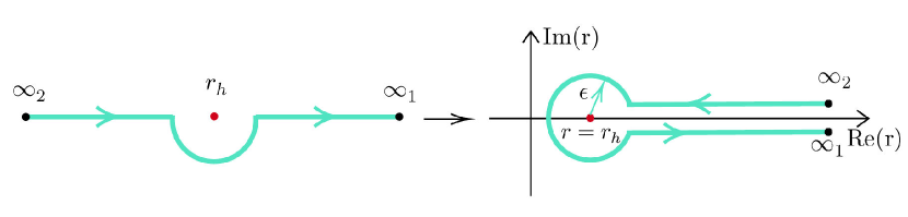
Figure 1: Left: complexified double AdS path (analytically continued near horizon) [55]; Right: the holographic SK contour [31]. Actually, the two horizontal legs overlap with the real axis.

The bulk equations of motion derived from (3.1) are

$$EL^{N}=0,\qquad ER^{N}=0,\qquad EX=0$$ (3.4)

where

$$EL^{M} =\nabla_{N}\left(F_{L}\right)^{MN}+{\rm i}\left[A_{LN},\left(F_{L}\right)^{NM}\right]+(\mathcal{J}_{L})^{M}$$

$$ER^{M} =\nabla_{N}\left(F_{R}\right)^{MN}+{\rm i}\left[A_{RN},\left(F_{R}\right)^{NM}\right]+(\mathcal{J}_{R})^{M}$$

$$EX =D^{M}(D_{M}X)-\left(m_{0}^{2}-\frac{\mu^{2}}{r^{2}}\right)X-2a\left(X^{{\dagger}}X\right)X$$ (3.5)

The bulk currents are

$$({\mathcal{J}}_{L})^{M} =-{\rm i}X\left(D^{M}X\right)^{{\dagger}}+{\rm i}\left(D_{M}X\right)X^{{\dagger}},$$

$$({\mathcal{J}}_{R})^{M} =-{\rm i}X^{\dagger}\left(D^{M}X\right)+{\rm i}\left(D_{M}X\right)^{{\dagger}}X$$ (3.6)

The bulk gauge symmetry allows us to take the following radial gauge condition [34]

$$A_{Lr}=-\frac{A_{L0}}{r^{2}f(r)},\qquad\qquad A_{Rr}=-\frac{A_{R0}}{r^{2}f(r)}.$$ (3.7)

Then, near the AdS boundary, the bulk fields behave as

$$A_{L\mu}\left(r\to\infty_{s},\ x^{\alpha}\right) =B_{s\mu}(x^{\alpha})+\cdots+\frac{\mathfrak{J}_{s\mu}(x^{\alpha})}{r^{2}}+\cdots,$$

$$A_{R\mu}\left(r\to\infty_{s},\ x^{\alpha}\right) =C_{s\mu}(x^{\alpha})+\cdots+\frac{\mathfrak{L}_{s\mu}(x^{\alpha})}{r^{2}}+\cdots,$$

$$X\left(r\to\infty_{s},\ x^{\alpha}\right) =\frac{m_{s}(x^{\alpha})}{r}+\cdots+\frac{\Sigma_{s}(x^{\alpha})}{r^{3}}+\cdots,$$ (3.8)

where $B_{s\mu}$, $C_{s\mu}$ and $\Sigma_{s}$ are exactly the dynamical variables introduced in section 2 for writing down the EFT action. Therefore, when solving bulk equations (3.4), we will impose boundary conditions as follows: take $B_{s\mu}$, $C_{s\mu}$ and $\Sigma_{s}$ as boundary data and fix them. So, once bulk equations are solved, the rest modes in (3.8) will become functionals of the boundary data.

It turns out that in order to fully determine the bulk gauge fields, we have to impose extra boundary conditions at the horizon [31]

$$A_{L0}(r=r_{h}-\epsilon,x^{\alpha})=0,\qquad A_{R0}(r=r_{h}-\epsilon,x^{\alpha})=0$$ (3.9)

which further breaks residual gauge invariance for bulk theory after taking the radial gauge condition (3.7). Physically, the horizon condition (3.9) corresponds to chemical shift symmetry for the boundary theory.

In order to remove divergences at $r=\infty$, we shall supplement the bulk action (3.1) with suitable counter-term action

$$S_{ct}=S_{ct}^{A}+S_{ct}^{X}$$ (3.10)

where

$$S_{ct}^{A}=\frac{1}{4}\log r\,\int d^{4}x\sqrt{-\gamma}{\rm Tr}\left(F_{L\mu\nu}F_{L}^{\mu\nu}+F_{R\mu\nu}F_{R}^{\mu\nu}\right),$$

$$S_{ct}^{X}=\int{d^{4}x}\sqrt{-\gamma}\,{\rm Tr}\left[n_{M}X^{{\dagger}}D^{M}X+n_{M}X(D^{M}X)^{{\dagger}}+X^{{\dagger}}X-(\overline{\nabla}_{\mu}X)^{{\dagger}}(\overline{\nabla}^{\mu}X)\log r\right],$$ (3.11)

where $r\to\infty$ is assumed. The counter-term action (3.11) is written down in minimal subtraction scheme. Here, $\gamma$ is the determinant of induced metric $\gamma_{\mu\nu}$ on the boundary $r=\infty$, $n_{M}$ is the normal vector of the hypersurface with $r=\infty$, and $\overline{\nabla}_{\mu}$ is the 4D covariant derivative compatible with the induced metric $\gamma_{\mu\nu}$.

In addition, we need to add a boundary term

$$S_{bdy}=\int{d^{4}x}\mathrm{Tr}\left(\frac{1}{2}m^{{\dagger}}\Box m-m^{{\dagger}}\partial_{0}^{2}m\right),$$ (3.12)

where $\Box=\eta^{\mu\nu}\partial_{\mu}\partial_{\nu}$ with $\eta^{\mu\nu}$ the 4D Minkowski metric. Eventually, the on-shell variation of the total bulk action reads

$$\delta(S_{0}+S_{ct}+S_{bdy})=\int d^{4}x{\rm Tr}\left(\mathfrak{J}_{s}^{\mu}\delta B_{s\mu}+\mathfrak{L}_{s}^{\mu}\delta C_{s\mu}-2m_{s}^{\dagger}\delta\Sigma_{s}-2m_{s}\delta\Sigma_{s}^{\dagger}\right)$$ (3.13)

which implies the bulk variational problem is well-defined given the boundary conditions specified below (3.8).

In the saddle point approximation, derivation of boundary effective action boils down to solving classical equations of motion for the bulk theory (3.4). However, to ensure the dynamical variables encoded in the boundary data off-shell, we will adopt a partially on-shell approach to solve the bulk dynamics, as demonstrated from bulk partition function [55, 35, 40]. Eventually, under the radial gauge choice (3.7), we will solve the dynamical components of bulk equations

$$EL^{0}-\frac{EL^{r}}{r^{2}f(r)}=0,\qquad EL^{0}-\frac{EL^{r}}{r^{2}f(r)}=0,\qquad EL^{i}=0,\qquad ER^{i}=0,\qquad EX=0$$ (3.14)

while leave aside the constraint equations

$$EL^{r}=0,\qquad ER^{r}=0$$ (3.15)

The boundary effective action is identified as

$$S_{eff}=S_{0}|_{p.o.s}+S_{ct}+S_{bdy}$$ (3.16)

where $S_{0}|_{p.o.s}$ stands for the partially on-shell bulk action obtained by plugging solutions for (3.14) into (3.1).

3.2 Bulk perturbation theory

In this section we set up a perturbative approach to solve the dynamical equations (3.14). Recall that the EFT action presented in section 2 is organized by number of dynamical fields $B_{s\mu}$, $C_{s\mu}$ and $\Sigma_{s}$ as well as number of spacetime derivatives of these fields. Accordingly, our strategy of for solving (3.14) will be through a double expansion.

First, we expand bulk fields as

$$A_{LM} =\alpha A_{LM}^{(1)}+\alpha^{2}A_{LM}^{(2)}+\cdots,\qquad A_{RM}=\alpha A_{RM}^{(1)}+\alpha^{2}A_{RM}^{(2)}+\cdots,$$

$$X =\alpha X^{(1)}+\alpha^{2}X^{(2)}+\cdots,$$ (3.17)

where the bookkeeping parameter $\alpha$ assists in counting number of dynamical variables $B_{s\mu}$, $C_{s\mu}$ and $\Sigma_{s}$. This can be viewed as linearization over the highly nonlinear system (3.14). Indeed, the leading order solutions $A_{LM}^{(1)}$ and $A_{RM}^{(1)}$ obey free Maxwell equations in the background spacetime (3.3). The nonlinear solutions like $A_{LM}^{(2)}$ and $A_{RM}^{(2)}$ obey similar equations as those of $A_{LM}^{(1)}$ and $A_{RM}^{(1)}$, with nontrivial sources to be built from lower order solutions. The conclusion also applies to the scalar field $X$: the leading part $X^{(1)}$ satisfies free Klein-Gordon (KG) equation in Schwarzschild-AdS₅, while the nonlinear parts like $X^{(2)}$ obey inhomogeneous KG equation with sources constructed from lower order solutions.

Next, at each order in the expansion (3.17), we do a boundary derivative expansion

$$A_{LM}^{(m)} =A_{LM}^{(m)(0)}+\lambda A_{LM}^{(m)(1)}+\lambda^{2}A_{LM}^{(m)(2)}+\cdots,$$

$$A_{RM}^{(m)} =A_{RM}^{(m)(0)}+\lambda A_{RM}^{(m)(1)}+\lambda^{2}A_{RM}^{(m)(2)}+\cdots,$$

$$X^{(m)} =X^{(m)(0)}+\lambda X^{(m)(1)}+\lambda^{2}X^{(m)(2)}+\cdots,$$ (3.18)

where $\lambda$ helps to count number of boundary derivatives.

Thanks to the double expansion (3.17) and (3.18), the dynamical equations (3.14) turn into a set of linear ordinary differential equations (ODEs) which we schematically write here

$$\Box_{0}A_{L0}^{(m)(n)}=j_{L0}^{(m)(n)},\qquad\Box_{i}A_{Li}^{(m)(n)}=j_{Li}^{(m)(n)},$$

$$\Box_{0}A_{R0}^{(m)(n)}=j_{R0}^{(m)(n)},\qquad\Box_{i}A_{Ri}^{(m)(n)}=j_{Ri}^{(m)(n)},$$

$$\Box_{X}X^{(m)(n)}=j_{X}^{(m)(n)}$$ (3.19)

where the differential operators can be read off from (3.14) by ignoring boundary spacetime derivatives

$$\Box_{0}=\partial_{r}(r^{3}\partial_{r}),\qquad\Box_{i}=\partial_{r}[r^{3}f(r)\partial_{r}],\qquad\Box_{X}=\partial_{r}[r^{5}f(r)\partial_{r}]-\left(m_{0}^{2}-\frac{\mu^{2}}{r^{2}}\right)$$ (3.20)

The source terms are easily read off by plugging the double expansion (3.17) and (3.18) into dynamical equations (3.14).

Perturbative solutions for the gauge sector

For the gauge sector, we can recycle our previous results for perturbative solutions [39, 40]. For the leading order parts, we have

$$A_{L0}^{(1)(0)}(r)=B_{s0}\left(1-\frac{r_{h}^{2}}{r^{2}}\right),\qquad r\in[r_{h}-\epsilon,\infty_{s}),$$

$$A_{L0}^{(1)(0)}(r)=C_{s0}\left(1-\frac{r_{h}^{2}}{r^{2}}\right),\qquad r\in[r_{h}-\epsilon,\infty_{s}),$$

$$A_{Li}^{(1)(0)}(r)=B_{2i}+\frac{B_{ai}}{2{\rm i}\pi}\log\frac{r^{2}-r_{h}^{2}}{r^{2}+r_{h}^{2}},$$

$$A_{Ri}^{(1)(0)}(r)=C_{2i}+\frac{C_{ai}}{2{\rm i}\pi}\log\frac{r^{2}-r_{h}^{2}}{r^{2}+r_{h}^{2}}$$ (3.21)

For the next to leading order parts, we have

$$A_{L0}^{(1)(1)}(r) =\frac{\partial_{0}B_{s0}}{4r_{h}}\left(1-\frac{r_{h}^{2}}{r^{2}}\right)\left[\pi-2\arctan\left(\frac{r}{r_{h}}\right)+\log\frac{r+r_{h}}{r-r_{h}}\right],\quad r\in[r_{h}-\epsilon,\infty_{s}),$$

$$A_{R0}^{(1)(1)}(r) =\frac{\partial_{0}C_{s0}}{4r_{h}}\left(1-\frac{r_{h}^{2}}{r^{2}}\right)\left[\pi-2\arctan\left(\frac{r}{r_{h}}\right)+\log\frac{r+r_{h}}{r-r_{h}}\right],\quad r\in[r_{h}-\epsilon,\infty_{s}),$$

$$A_{Li}^{(1)(1)}(r) =\frac{\partial_{0}B_{2i}}{4r_{h}}\left[\pi-2\arctan\left(\frac{r}{r_{h}}\right)+2\log(r+r_{h})-\log(r^{2}+r_{h}^{2})\right]$$

$$-\frac{\partial_{0}B_{ai}}{8\pi r_{h}}\left[-(2-{\rm i})\pi-2{\rm i}\arctan\left(\frac{r}{r_{h}}\right)-{\rm i}\log\frac{r-r_{h}}{r+r_{h}}\right]\log\frac{r^{2}-r_{h}^{2}}{r^{2}+r_{h}^{2}},$$

$$A_{Ri}^{(1)(1)}(r) =\frac{\partial_{0}C_{2i}}{4r_{h}}\left[\pi-2\arctan\left(\frac{r}{r_{h}}\right)+2\log(r+r_{h})-\log(r^{2}+r_{h}^{2})\right]$$

$$-\frac{\partial_{0}C_{ai}}{8\pi r_{h}}\left[-(2-{\rm i})\pi-2{\rm i}\arctan\left(\frac{r}{r_{h}}\right)-{\rm i}\log\frac{r-r_{h}}{r+r_{h}}\right]\log\frac{r^{2}-r_{h}^{2}}{r^{2}+r_{h}^{2}}.$$ (3.22)

For higher order solutions, instead of recording lengthy expressions, we write them compactly as radial integrals. For time-components, we have

$$A_{L0}^{(m)(n)}(r)=\int_{\infty_{s}}^{r}\left[\frac{1}{x^{3}}\int_{\infty_{s}}^{x}j_{L0}^{(m)(n)}(y)dy+\frac{c_{s}^{(m)(n)}}{x^{3}}\right]dx,\quad r\in[r_{h}-\epsilon,\infty_{s}),$$

$$A_{R0}^{(m)(n)}(r)=\int_{\infty_{s}}^{r}\left[\frac{1}{x^{3}}\int_{\infty_{s}}^{x}j_{R0}^{(m)(n)}(y)dy+\frac{d_{s}^{(m)(n)}}{x^{3}}\right]dx,\quad\,\,r\in[r_{h}-\epsilon,\infty_{s}),$$ (3.23)

where the integration constants $c_{s}^{(m)(n)}$ and $d_{s}^{(m)(n)}$ are determined by vanishing horizon condition (3.9).

For spatial components, we have

$$A_{Li}^{(m)(n)}(r) =\int_{\infty_{2}}^{\infty_{1}}G_{Y}(r,\xi)j_{Li}^{(m)(n)}(\xi)d\xi$$

$$=\frac{Y_{1}(r)}{2{\rm i}\pi r_{h}^{2}}\int_{\infty_{2}}^{r}Y_{2}(\xi)j_{i}^{(m)(n)}(\xi)d\xi+\frac{Y_{2}(r)}{2{\rm i}\pi r_{h}^{2}}\int_{r}^{\infty_{1}}Y_{1}(\xi)j_{Li}^{(m)(n)}(\xi)d\xi,$$

$$A_{Ri}^{(m)(n)}(r) =\int_{\infty_{2}}^{\infty_{1}}G_{Y}(r,\xi)j_{Ri}^{(m)(n)}(\xi)d\xi$$

$$=\frac{Y_{1}(r)}{2{\rm i}\pi r_{h}^{2}}\int_{\infty_{2}}^{r}Y_{2}(\xi)j_{Ri}^{(m)(n)}(\xi)d\xi+\frac{Y_{2}(r)}{2{\rm i}\pi r_{h}^{2}}\int_{r}^{\infty_{1}}Y_{1}(\xi)l_{i}^{(m)(n)}(\xi)d\xi,$$ (3.24)

where $Y_{1}(r)$ and $Y_{2}(r)$ are two linearly independent solutions for homogeneous part of (3.19) which we take as [39, 40]

$$Y_{1}(r)=-\frac{1}{2}\log\frac{r^{2}-r_{h}^{2}}{r^{2}+r_{h}^{2}}+{\rm i}\pi,\qquad\qquad Y_{2}(r)=-\frac{1}{2}\log\frac{r^{2}-r_{h}^{2}}{r^{2}+r_{h}^{2}}.$$ (3.25)

Perturbative solutions for the scalar sector

Regarding the scalar sector, we resort to a numerical technique since it is impossible to have analytical solutions. First, we consider the linear solution $X^{(1)}$ in the expansion (3.17). In the Fourier space achieved by $\partial_{\mu}\to{\rm i}k_{\mu}=(-{\rm i}\omega,{\rm i}\vec{q}\,)$, the equation of motion for $X^{(1)}$ is

$$\partial_{r}\left[r^{5}f(r)\partial_{r}X^{(1)}\right]-\left(m_{0}^{2}-\frac{\mu^{2}}{r^{2}}\right)r^{3}X^{(1)}-2{\rm i}\omega r^{3}\partial_{r}X^{(1)}-3{\rm i}\omega r^{2}X^{(1)}-q^{2}rX^{(1)}=0$$ (3.26)

Following the idea of [33, 36, 38], the solution for $X^{(1)}$ is

$$X^{(1)}(r,k_{\mu}) =\left[\frac{1}{2}\coth\left(\frac{\beta\omega}{2}\right)\Sigma_{a}(k_{\mu})+\Sigma_{r}(k_{\mu})\right]\frac{\Phi(r,k_{\mu})}{\Phi^{(3)}(k_{\mu})}$$

$$-\Sigma_{a}(k_{\mu})\frac{e^{2{\rm i}\omega\chi(r)}}{(1-e^{-\beta\omega})}\frac{\Phi(r,-k_{\mu})}{\Phi^{(3)}(-k_{\mu})}$$ (3.27)

Here, $\Phi(r,k_{\mu})$ is a regular solution (i.e., the ingoing mode) for the linear equation (3.26), which will be constructed numerically [38]. Near the AdS boundary $r=\infty$, the regular solution $\Phi(r,k_{\mu})$ is expanded as

$$\Phi(r\to\infty,k_{\mu})=\cdots+\frac{\Phi^{(3)}(k_{\mu})}{r^{3}}+\cdots$$ (3.28)

The factor $\chi(r)$ is

$$\chi(r)\equiv\int_{\infty_{2}}^{r}\frac{dy}{y^{2}f(y)}=-\frac{1}{4r_{h}}\left[\pi-2\arctan\left(\frac{r}{r_{h}}\right)+\log\left(1+\frac{r_{h}}{r}\right)-\log\left(1-\frac{r_{h}}{r}\right)\right]$$ (3.29)

Based on the linear solution (3.27), the higher order solutions can be constructed via Green’s function method as implemented for the gauge sector, see (3.24). Here, the two linearly independent solutions $\tilde{Z}_{1}(r)$ and $\tilde{Z}_{2}(r)$ for the homogeneous equation $\Box_{X}=0$ can be extracted from (3.27). The result is

$$\tilde{Z}_{1}(r)=\Phi_{0}(r),\qquad\tilde{Z}_{2}(r)=\chi(r)\Phi_{0}(r)-\Phi_{1}(r)$$ (3.30)

where $\Phi_{0}(r)$ and $\Phi_{1}(r)$ correspond to hydrodynamic expansion of the regular solution $\Phi(r,k_{\mu})$

$$\Phi(r,k_{\mu}\to 0)=\Phi_{0}(r)+{\rm i}\omega\Phi_{1}(r)+\cdots$$ (3.31)

In practice, we make linear combination of $\tilde{Z}_{1}(r)$ and $\tilde{Z}_{2}(r)$ and generate two new linear solutions

$$Z_{1}(r)=g_{1}\tilde{Z}_{1}(r)+g_{2}\tilde{Z}_{2}(r),\qquad Z_{2}(r)=h_{1}\tilde{Z}_{1}(r)+h_{2}\tilde{Z}_{2}(r)$$ (3.32)

which near the AdS boundary have “ideal” asymptotic behaviors

$$Z_{1}(r\to\infty_{1})=\frac{1}{r}+\cdots+\frac{0}{r^{3}}+\cdots,\qquad Z_{2}(r\to\infty_{2})=\frac{0}{r}+\cdots+\frac{1}{r^{3}}+\cdots$$ (3.33)

Recall that we will focus on the regime near the phase transition so that we can take (3.2). So, throughout our holographic derivation of the EFT action presented in section 2, our computation will be limited to the critical point $\mu=\mu_{c}$ except for $b_{0}$ which requires a tiny deviation $\delta\mu$. When $\mu=\mu_{c}$ (at the critical point), the numerical values for $g_{1,2},h_{1,2}$ of (3.32) are

$$g_{1}=-15.04-5.34\text{i},\quad g_{2}=3.40,\quad h_{1}=-15.04,\quad h_{2}=3.40$$ (3.34)

Now, we present the solutions for higher order parts for scalar sector

$$X^{(m)(n)}(r) =\int_{\infty_{2}}^{\infty_{1}}dr^{\prime}G_{X}(r,r^{\prime})j_{X}^{(m)(n)}(r^{\prime})dr^{\prime}$$

$$=\frac{Z_{1}(r)}{\mathcal{C}}\int_{\infty_{2}}^{r}Z_{2}(r^{\prime})j_{X}^{(m)(n)}(r^{\prime})dr^{\prime}+\frac{Z_{2}(r)}{\mathcal{C}}\int_{r}^{\infty_{1}}Z_{1}(r^{\prime})j_{X}^{(m)(n)}(r^{\prime})dr^{\prime},$$ (3.35)

where $G_{X}(r,r^{\prime})$ is the Green’s function. The constant $\mathcal{C}$ is determined from Wronskian determinant of $Z_{1}(r)$ and $Z_{2}(r)$

$$W_{Z}\equiv Z_{2}(r)\partial_{r}Z_{1}(r)-Z_{1}(r)\partial_{r}Z_{2}(r)=\frac{\mathcal{C}}{r^{5}f(r)}\Longrightarrow\mathcal{C}=18.17{\rm i}$$ (3.36)

3.3 Holographic effective action

In this section, we compute the boundary effective action based on the perturbative solutions obtained in last section 3.2.

In accord with the expansion of (3.17), the gauge field strength $F_{L}$ can be expanded as (similarly for $F_{R}$)

$$F_{L}=\alpha F_{L}^{(1)}+\alpha^{2}F_{L}^{(2)}+\alpha^{3}F_{L}^{(3)}+\cdots$$ (3.37)

where for simplicity we ignored both Lorentzian indices and flavor indices. In the bulk action, the contribution from the gauge field strengths is

$$S_{F} =-\frac{1}{4}\int d^{5}x\sqrt{-g}\,{\rm Tr}\left(F_{L}^{2}+F_{R}^{2}\right)+S_{ct}^{A}$$

$$=-\frac{1}{4}\int d^{5}x\sqrt{-g}\,{\rm Tr}\left[\left(F_{L}^{(1)}\right)^{2}+2F_{L}^{(1)}F_{L}^{(2)}+2F_{L}^{(1)}F_{L}^{(3)}+\left(F_{L}^{(2)}\right)^{2}+\cdots\right.$$

$$\qquad\qquad\qquad\qquad\quad\,\,\left.\left(F_{R}^{(1)}\right)^{2}+2F_{R}^{(1)}F_{R}^{(2)}+2F_{R}^{(1)}F_{R}^{(3)}+\left(F_{R}^{(2)}\right)^{2}+\cdots\right]+S_{ct}^{A}$$ (3.38)

Then, based on (3.38), it can be demonstrated that [37] the linear solutions $A_{L}^{(1)}$ and $A_{R}^{(1)}$ are sufficient in calculating boundary action up to order $\mathcal{O}(\alpha^{4})$. Moreover, the terms of order $\mathcal{O}(\alpha^{4})$ in (3.38) contain at least one boundary derivative, which we have not covered in section 2. Therefore, the contribution from $S_{F}$ could be simply computed as

$$S_{F}=-\frac{1}{4}\int d^{4}x\int_{\infty_{2}}^{\infty_{1}}dr\sqrt{-g}\left(F_{L}^{2}+F_{R}^{2}\right)\bigg{|}_{A_{L}\to A_{L}^{(1)},\,A_{R}\to A_{R}^{(1)}}+S_{ct}^{A}$$ (3.39)

where the linear solutions $A_{L}^{(1)}$ and $A_{R}^{(1)}$ are presented in (3.21) through (3.24). Evaluating the radial integral in (3.39), we obtain exactly (2.20) and the last four terms of (2.24) with holographic results for various coefficients [34, 40]

$$a_{0}=2r_{h}^{2},\quad a_{1}=0,\quad a_{2}=-r_{h},\quad a_{3}=-\frac{\log(2r_{h}^{2}/L^{2})}{2},\quad a_{4}=-\frac{\log(2r_{h}^{2}/L^{2})}{2},$$

$$a_{5}=\log(2r_{h}^{2}/L^{2}),\quad a_{6}=\frac{1}{2}\log(r_{h}^{2}/L^{2}),\quad a_{7}=2r_{h}^{2},\quad a_{8}=0,\quad a_{9}=-r_{h},$$

$$a_{10}=-\frac{\log(2r_{h}^{2}/L^{2})}{2},\quad a_{11}=-\frac{\log(2r_{h}^{2}/L^{2})}{2},\quad a_{12}=\log(2r_{h}^{2}/L^{2}),\quad a_{13}=\frac{1}{2}\log(r_{h}^{2}/L^{2}),$$

$$\varpi_{1}=\varpi_{2}=\log(2r_{h}/L),\qquad\varpi_{3}=\varpi_{4}=-\log(2r_{h}^{2}/L^{2})$$ (3.40)

where we recovered AdS radius $L$ by dimensional analysis. As pointed out in [39], the fact that $a_{1}=0$ and $a_{8}=0$ is related to the hydrodynamic frame that holographic model naturally choose. In other words, $a_{1}$ and $a_{8}$ can be consistently set to zero by appropriate field redefinition, at the cost of having an additional higher order terms [39, 21]. The results for $a_{6}$ and $a_{13}$ are renormalization scheme-dependent, see (3.11).

We turn to the contribution from scalar sector in the bulk action (3.1)

$$S_{X} \equiv\int d^{5}x\sqrt{-g}\,{\rm Tr}\left\{-\left|DX\right|^{2}-\left(m_{0}^{2}-\frac{\mu_{c}^{2}}{r^{2}}\right)|X|^{2}-a|X|^{4}\right\}+S_{ct}^{X}+S_{bdy}$$

$$=-\int d^{4}x\mathrm{Tr}\left(r^{5}X^{\dagger}\partial_{r}X+r^{3}X^{\dagger}\partial_{0}X\right)\bigg{|}_{r=\infty_{2}}^{r=\infty_{1}}+a\int d^{5}x\sqrt{-g}\,{\rm Tr}(|X|^{4})$$

$$=\int d^{4}x\,{\rm Tr}\left(2m_{1}^{\dagger}\Sigma_{1}-2m_{2}^{\dagger}\Sigma_{2}\right)+a\int d^{5}x\sqrt{-g}\,{\rm Tr}\left(|X|^{4}\right)$$

$$=\int d^{4}x\,{\rm Tr}\left[(m_{1}+m_{2})^{\dagger}\Sigma_{a}+2(m_{1}-m_{2})^{\dagger}\Sigma_{r}\right]+a\int d^{5}x\sqrt{-g}\,{\rm Tr}\left(|X|^{4}\right),$$ (3.41)

where in the second equality we have integrated by part and made use of scalar’s equation of motion. The $m_{1,2}$ are leading terms in the near boundary asymptotic behavior for $X$, see (3.8). In accord with the expansions (3.17) and (3.18), we expand $m_{s}$ formally

$$m_{s} =\alpha\,m_{s}^{(1)}+\alpha^{2}m^{(2)}_{s}+\alpha^{3}m^{(3)}+\cdots,$$

$$m_{s}^{(l)} =m_{s}^{(l)(0)}+\lambda^{1}m_{s}^{(l)(1)}+\lambda^{2}m_{s}^{(l)(2)}+\cdots$$ (3.42)

From the linear solution $X^{(1)}$ in (3.27), it is straightforward to read off $m_{s}^{(1)}$. In the hydrodynamic limit, they are expanded as

$$\left(m_{1}^{(1)}\right)^{\dagger}+\left(m_{2}^{(1)}\right)^{\dagger} =0.2904(\mu_{c}-\mu)\Sigma_{r}^{\dagger}+(0.348+0.01{\rm i})\partial_{0}\Sigma_{r}^{\dagger}-0.121\partial_{i}^{2}\Sigma_{r}^{\dagger}$$

$$\quad+(0.022+0.100{\rm i})\partial_{0}^{2}\Sigma_{r}^{\dagger}+\cdots,$$

$$2\left[\left(m_{1}^{(1)}\right)^{\dagger}-\left(m_{2}^{(1)}\right)^{\dagger}\right] =0.2904(\mu_{c}-\mu)\Sigma_{a}^{\dagger}-(0.348+0.01{\rm i})\partial_{0}\Sigma_{a}^{\dagger}-0.121\partial_{i}^{2}\Sigma_{a}^{\dagger}$$

$$\quad-(0.022+0.100{\rm i})\partial_{0}^{2}\Sigma_{a}^{\dagger}+\cdots.$$ (3.43)

Then, plugging (3.43) into (3.41), we perfectly produce quadratic terms of (2.23). The holographic results for various coefficients of (2.23) are (in unit of $r_{h}=1$)

$$b_{0}=0.290(\mu_{c}-\mu),\quad b_{1}=-0.348-0.0100{\rm i},\quad b_{2}=-0.121,\quad b_{3}=-0.022-0.100{\rm i},$$ (3.44)

where by dimensional analysis $(\mu_{c}-\mu)\sim(T-T_{c})$ with $T_{c}$ the critical temperature.

We turn to cubic terms of the boundary action, which generically contain both zeroth and first order derivatives. From holographic formula (3.41), this requires to compute $m_{1}^{(2)(0)}$ and $m_{1}^{(2)(1)}$. The latter can be extracted from the formal expressions (3.35)

$$m_{1}^{(2)(n)}=\frac{1}{\mathcal{C}}\int_{\infty_{2}}^{\infty_{1}}Z_{2}(r^{\prime})j_{X}^{(2)(n)}(r^{\prime})dr^{\prime},\qquad m_{2}^{(2)(n)}=\frac{1}{\mathcal{C}}\int_{\infty_{2}}^{\infty_{1}}Z_{1}(r^{\prime})j_{X}^{(2)(n)}(r^{\prime})dr^{\prime}$$ (3.45)

where $n=0,1$. Here, the relevant sources can be read off from the bulk equations

$$j_{X}^{(2)(0)} =0,$$

$$j_{X}^{(2)(1)} =-2{\rm i}rA_{Li}^{(1)(0)}\partial_{i}X^{(1)(0)}+2{\rm i}r\partial_{i}X^{(1)(0)}A_{Ri}^{(1)(0)}-{\rm i}r\partial_{i}A_{Li}^{(1)(0)}X^{(1)(0)}$$

$$\quad+{\rm i}rX^{(1)(0)}\partial_{i}A_{Ri}^{(1)(0)}$$ (3.46)

With $A_{L,R}^{(1)(0)}$ presented in (3.21) and $X^{(1)(0)}$ easily extracted from (3.27), we work out the radial integrals of (3.45) numerically:

$$\left(m_{1}^{(2)}\right)^{\dagger}+\left(m_{2}^{(2)}\right)^{\dagger} =0.242{\rm i}\left(\partial_{i}\Sigma_{r}^{{\dagger}}B_{ri}-C_{ri}\partial_{i}\Sigma_{r}^{{\dagger}}\right)+0.121{\rm i}\left(\Sigma_{r}^{{\dagger}}\partial_{i}B_{ri}-\partial_{i}C_{ri}\Sigma_{r}^{{\dagger}}\right)$$

$$2\left[\left(m_{1}^{(2)}\right)^{\dagger}-\left(m_{2}^{(2)}\right)^{\dagger}\right] =0.242{\rm i}\left(\partial_{i}\Sigma_{r}^{{\dagger}}B_{ai}+\partial_{i}\Sigma_{a}^{{\dagger}}B_{ri}-C_{ai}\partial_{i}\Sigma_{r}^{{\dagger}}-C_{ri}\partial_{i}\Sigma_{a}^{{\dagger}}\right)$$

$$\quad+0.121{\rm i}\left(\Sigma_{r}^{{\dagger}}\partial_{i}B_{ai}+\Sigma_{a}^{{\dagger}}\partial_{i}B_{ri}-\partial_{i}C_{ai}\Sigma_{r}^{{\dagger}}-\partial_{i}C_{ri}\Sigma_{a}^{{\dagger}}\right).$$ (3.47)

Finally, we compute quartic terms of the boundary action. The holographic formula (3.41) implies two sources for quartic terms. The first one corresponds to bulk part of (3.41), which is computed as

$$\int_{\infty_{2}}^{\infty_{1}}dr\sqrt{-g}\,|X|^{4}\bigg{|}_{X\to X^{(1)(0)}}$$

$$= 0.0449\Sigma_{r}\Sigma_{a}^{{\dagger}}\Sigma_{r}\Sigma_{r}^{{\dagger}}+0.0449\Sigma_{r}\Sigma_{r}^{{\dagger}}\Sigma_{a}\Sigma_{r}^{{\dagger}}$$ (3.48)

The second source of quartic terms comes from the first part of (3.41), which requires to compute $m_{s}^{(3)(0)}$

$$m_{1}^{(3)(0)}=\frac{1}{\mathcal{C}}\int_{\infty_{2}}^{\infty_{1}}Z_{2}(r^{\prime})j_{X}^{(3)(0)}(r^{\prime})dr^{\prime},\qquad m_{2}^{(3)(0)}=\frac{1}{\mathcal{C}}\int_{\infty_{2}}^{\infty_{1}}Z_{1}(r^{\prime})j_{X}^{(3)(0)}(r^{\prime})dr^{\prime}$$ (3.49)

Here, the relevant source terms are

$$j_{X}^{(3)(0)} =\frac{r}{f(r)}A_{L0}^{2}X+\frac{r}{f(r)}XA_{R0}^{2}-\frac{2r}{f(r)}A_{L0}XA_{R0}-rA_{Li}A_{Li}X$$

$$\quad-rXA_{Ri}A_{Ri}+2rA_{Li}XA_{Ri}+2aX^{\dagger}XX\bigg{|}_{A_{L,R}\to A_{L,R}^{(1)(0)},\,X\to X^{(1)(0)}}$$ (3.50)

Working out the radial integrals in (3.49), we have

$$\left(m_{1}^{(2)}\right)^{\dagger}+\left(m_{2}^{(2)}\right)^{\dagger} =0.0336\left(\Sigma_{r}^{{\dagger}}B_{r0}B_{r0}+C_{r0}C_{r0}\Sigma_{r}^{{\dagger}}-2C_{r0}\Sigma_{r}^{{\dagger}}B_{r0}\right)$$

$$-0.121\left(\Sigma_{r}^{{\dagger}}B_{ri}B_{ri}+C_{ri}C_{ri}\Sigma_{r}^{{\dagger}}-2C_{ri}\Sigma_{r}^{{\dagger}}B_{ri}\right)$$

$$-0.0293a\Sigma_{r}^{{\dagger}}\Sigma_{r}\Sigma_{r}^{{\dagger}}$$

$$2\left[\left(m_{1}^{(2)}\right)^{\dagger}-\left(m_{2}^{(2)}\right)^{\dagger}\right] =0.0336\left(\Sigma_{a}^{{\dagger}}B_{r0}B_{r0}+C_{r0}C_{r0}\Sigma_{a}^{{\dagger}}-2C_{r0}\Sigma_{a}^{{\dagger}}B_{r0}+2\Sigma_{r}^{{\dagger}}B_{a0}B_{r0}\right.$$

$$\qquad\qquad\,\,\left.+2C_{a0}C_{r0}\Sigma_{r}^{{\dagger}}-2C_{a0}\Sigma_{r}^{{\dagger}}B_{r0}-2C_{r0}\Sigma_{r}^{{\dagger}}B_{a0}\right)$$

$$-0.121\left(\Sigma_{a}^{{\dagger}}B_{ri}B_{ri}+C_{ri}C_{ri}\Sigma_{a}^{{\dagger}}-2C_{ri}\Sigma_{a}^{{\dagger}}B_{ri}+\Sigma_{r}^{{\dagger}}B_{ri}B_{ai}+\Sigma_{r}^{{\dagger}}B_{ai}B_{ri}\right.$$

$$\qquad\qquad\left.+C_{ai}C_{ri}\Sigma_{r}^{{\dagger}}+C_{ri}C_{ai}\Sigma_{r}^{{\dagger}}-2C_{ai}\Sigma_{r}^{{\dagger}}B_{ri}-2C_{ri}\Sigma_{r}^{{\dagger}}B_{ai}\right)$$

$$-0.0293a\Sigma_{r}^{{\dagger}}\Sigma_{r}\Sigma_{a}^{{\dagger}}$$ (3.51)

Plugging (3.47), (3.48) and (3.51) into (3.41), we read off holographic results for the coefficients in cubic terms (2.24) and quartic terms (2.27) (in unit of $r_{h}$)

$$c_{0}=c_{1}=0,\quad d_{0}=d_{1}=0,\quad c_{2}=0.121,\quad d_{2}=-0.121,$$

$$c_{3}=c_{3}^{*}=2c_{4}=2c_{4}^{*}=0.0672,\quad d_{3}=d_{3}^{*}=2d_{4}=2d_{4}^{*}=0.0672,$$

$$\chi_{1}=0.0156a,\quad\chi_{2}=-0.134,\quad\chi_{3}=-0.134,\quad\chi_{4}=\chi_{4}^{*}=-0.0672.$$ (3.52)

Our holographic results satisfy all the symmetries summarized in section 2.1. In particular, owing to the chemical shift symmetry, we see that some quadratic terms, cubic terms and quartic terms (i.e., those terms hidden behind the covariant spatial derivative $\mathcal{D}_{i}$ in (2.23) and (2.24)) are linked to each other sharing the same coefficients. This is clearly obeyed by our numerical results, as shown in (3.43) (spatial derivative terms), (3.47) and relevant parts (i.e., the second line, the sixth line, and the seventh line) in (3.51).

Notice that the holographic model gives $c_{0}=c_{1}=0$ and $d_{0}=d_{1}=0$. However, this shall be understood as an accidental issue arising from the saddle point approximation undertaken in this work. This is directly related to the fact that vertices like $XXA_{L0}$ and $XXA_{R0}$ are absent in the bulk theory, as seen from the first line of the formula (3.46). However, beyond probe limit, such terms would be generated through loop effects in the bulk, as illustrated by the Witten diagram of Figure 2.

Figure 2: Witten diagram for $B_{0}\Sigma\Sigma^{\dagger}$-terms in boundary action. Left: they would not vanish if loop effects are considered in the bulk theory. Right: they do vanish at the tree level of the bulk theory in the probe limit.

4 Summary and Outlook

We have constructed a Wilsonian EFT (in a real-time formalism) which is valid for studying the long-wavelength lone-time dynamics of QCD matter near the chiral phase transition. The dynamical variables contain conserved charge densities associated with the chiral symmetry and the order parameter characterising the $\chi$SB. The inclusion of the latter as a dynamical field is crucial as one focuses on critical regime of chiral phase transition. The EFT Lagrangian is stringently constrained by the set of symmetries postulated for hydrodynamic EFT [20, 21, 24], in particular, the dynamical KMS symmetry and the chemical shift symmetry, which link certain terms in the EFT action. From the EFT action, we have derived a set of stochastic equations for the chiral charge densities and the chiral condensate, which will be useful for numerical simulations. We found that, with higher order terms ignored properly, the set of stochastic equations resemble the model F of Hohenberg-Halperin classification [10], which was proposed to study dynamical evolution of critical U(1) superfluid system. The EFT approach provides a systematic way of extending phenomenological stochastic models.

By applying the holographic Schwinger-Keldysh technique [31], we have confirmed the EFT construction by deriving boundary effective action for a modified AdS/QCD model [49, 50, 51, 17]. The modified AdS/QCD naturally incorporates spontaneous $\chi$SB and thus allows to get access into critical regime of chiral phase transition. Moreover, the holographic study gives valuable information on parameters in the EFT action, whose microscopic theory is strongly coupled and is usually channelling to study with perturbative method. Intriguingly, we find some coefficients (i.e., $c_{0,1}$ and $d_{0,1}$ in (2.24)) are accidentally zero. We attribute this to the saddle point approximation and the probe limit undertaken in this work.

There are several directions we hope to address in the future. First, it will be interesting to explore consequences of higher order terms in (2.38), i.e., those beyond model F in Hohenberg-Halperin classification, along the line of [56]. This might be important in clarifying non-Gaussianity regarding QCD critical point. Second, it would be straightforward to include effect of explicit breaking of chiral symmetry in the spirit of [47], which utilized a spurious symmetry by associating a transformation rule for mass matrix (as a source for the order parameter $\Sigma$). Presumably, this effect will render the transition into a crossover. Third, the EFT constructed in this work would be useful in understanding phases of nuclear matter at finite temperature and isospin chemical potential, such as Pion superfluid phase (i.e., Pion condensation). Last but not the least, it will be interesting to consider more realistic AdS/QCD models such as [57, 58, 59, 60] that have taken into account latest lattice results, observational constraints, etc. Study along this line is supposed to provide more realistic information for the parameters appearing in the low energy EFT.

References

- [1] A. Jaiswal et al., “Dynamics of QCD matter — current status,” Int. J. Mod. Phys. E 30 no. 02, (2021) 2130001, arXiv:2007.14959 [hep-ph].
- [2] MUSES Collaboration, R. Kumar et al., “Theoretical and experimental constraints for the equation of state of dense and hot matter,” Living Rev. Rel. 27 no. 1, (2024) 3, arXiv:2303.17021 [nucl-th].
- [3] A. M. Halasz, A. D. Jackson, R. E. Shrock, M. A. Stephanov, and J. J. M. Verbaarschot, “On the phase diagram of QCD,” Phys. Rev. D 58 (1998) 096007, arXiv:hep-ph/9804290.
- [4] A. Bzdak, S. Esumi, V. Koch, J. Liao, M. Stephanov, and N. Xu, “Mapping the Phases of Quantum Chromodynamics with Beam Energy Scan,” Phys. Rept. 853 (2020) 1–87, arXiv:1906.00936 [nucl-th].
- [5] L. Du, A. Sorensen, and M. Stephanov, “The QCD phase diagram and Beam Energy Scan physics: a theory overview,” Int. J. Mod. Phys. E 33 no. 07, (2024) 2430008, arXiv:2402.10183 [nucl-th].
- [6] X. Luo, S. Shi, N. Xu, and Y. Zhang, “A Study of the Properties of the QCD Phase Diagram in High-Energy Nuclear Collisions,” Particles 3 no. 2, (2020) 278–307, arXiv:2004.00789 [nucl-ex].
- [7] Q.-Y. Shou et al., “Properties of QCD matter: a review of selected results from ALICE experiment,” Nucl. Sci. Tech. 35 no. 12, (2024) 219, arXiv:2409.17964 [nucl-ex].
- [8] R. D. Pisarski and F. Wilczek, “Remarks on the Chiral Phase Transition in Chromodynamics,” Phys. Rev. D 29 (1984) 338–341.
- [9] K. Rajagopal and F. Wilczek, “Static and dynamic critical phenomena at a second order QCD phase transition,” Nucl. Phys. B 399 (1993) 395–425, arXiv:hep-ph/9210253.
- [10] P. C. Hohenberg and B. I. Halperin, “Theory of dynamic critical phenomena,” Rev. Mod. Phys. 49 (Jul, 1977) 435–479. https://link.aps.org/doi/10.1103/RevModPhys.49.435.
- [11] D. T. Son and M. A. Stephanov, “Real time pion propagation in finite temperature QCD,” Phys. Rev. D 66 (2002) 076011, arXiv:hep-ph/0204226.
- [12] D. T. Son and M. A. Stephanov, “Pion propagation near the QCD chiral phase transition,” Phys. Rev. Lett. 88 (2002) 202302, arXiv:hep-ph/0111100.
- [13] D. T. Son, “Hydrodynamics of nuclear matter in the chiral limit,” Phys. Rev. Lett. 84 (2000) 3771–3774, arXiv:hep-ph/9912267.
- [14] E. Grossi, A. Soloviev, D. Teaney, and F. Yan, “Transport and hydrodynamics in the chiral limit,” Phys. Rev. D 102 no. 1, (2020) 014042, arXiv:2005.02885 [hep-th].
- [15] E. Grossi, A. Soloviev, D. Teaney, and F. Yan, “Soft pions and transport near the chiral critical point,” Phys. Rev. D 104 no. 3, (2021) 034025, arXiv:2101.10847 [nucl-th].
- [16] A. Florio, E. Grossi, A. Soloviev, and D. Teaney, “Dynamics of the critical point in QCD,” Phys. Rev. D 105 no. 5, (2022) 054512, arXiv:2111.03640 [hep-lat].
- [17] X. Cao, M. Baggioli, H. Liu, and D. Li, “Pion dynamics in a soft-wall AdS-QCD model,” JHEP 12 (2022) 113, arXiv:2210.09088 [hep-ph].
- [18] J. Braun et al., “Soft modes in hot QCD matter,” arXiv:2310.19853 [hep-ph].
- [19] J. V. Roth, Y. Ye, S. Schlichting, and L. von Smekal, “Dynamic critical behavior of the chiral phase transition from the real-time functional renormalization group,” arXiv:2403.04573 [hep-ph].
- [20] M. Crossley, P. Glorioso, and H. Liu, “Effective field theory of dissipative fluids,” JHEP 09 (2017) 095, arXiv:1511.03646 [hep-th].
- [21] P. Glorioso, M. Crossley, and H. Liu, “Effective field theory of dissipative fluids (II): classical limit, dynamical KMS symmetry and entropy current,” JHEP 09 (2017) 096, arXiv:1701.07817 [hep-th].
- [22] F. M. Haehl, R. Loganayagam, and M. Rangamani, “Topological sigma models & dissipative hydrodynamics,” JHEP 04 (2016) 039, arXiv:1511.07809 [hep-th].
- [23] F. M. Haehl, R. Loganayagam, and M. Rangamani, “Effective Action for Relativistic Hydrodynamics: Fluctuations, Dissipation, and Entropy Inflow,” JHEP 10 (2018) 194, arXiv:1803.11155 [hep-th].
- [24] H. Liu and P. Glorioso, “Lectures on non-equilibrium effective field theories and fluctuating hydrodynamics,” PoS 305 (2018) 008, arXiv:1805.09331 [hep-th].
- [25] J. M. Maldacena, “The Large N limit of superconformal field theories and supergravity,” Adv. Theor. Math. Phys. 2 (1998) 231–252, arXiv:hep-th/9711200.
- [26] S. S. Gubser, I. R. Klebanov, and A. M. Polyakov, “Gauge theory correlators from noncritical string theory,” Phys. Lett. B 428 (1998) 105–114, arXiv:hep-th/9802109.
- [27] E. Witten, “Anti-de Sitter space and holography,” Adv. Theor. Math. Phys. 2 (1998) 253–291, arXiv:hep-th/9802150.
- [28] C. P. Herzog and D. T. Son, “Schwinger-Keldysh propagators from AdS/CFT correspondence,” JHEP 03 (2003) 046, arXiv:hep-th/0212072.
- [29] K. Skenderis and B. C. van Rees, “Real-time gauge/gravity duality,” Phys. Rev. Lett. 101 (2008) 081601, arXiv:0805.0150 [hep-th].
- [30] K. Skenderis and B. C. van Rees, “Real-time gauge/gravity duality: Prescription, Renormalization and Examples,” JHEP 05 (2009) 085, arXiv:0812.2909 [hep-th].
- [31] P. Glorioso, M. Crossley, and H. Liu, “A prescription for holographic Schwinger-Keldysh contour in non-equilibrium systems,” arXiv:1812.08785 [hep-th].
- [32] J. de Boer, M. P. Heller, and N. Pinzani-Fokeeva, “Holographic Schwinger-Keldysh effective field theories,” JHEP 05 (2019) 188, arXiv:1812.06093 [hep-th].
- [33] B. Chakrabarty, J. Chakravarty, S. Chaudhuri, C. Jana, R. Loganayagam, and A. Sivakumar, “Nonlinear Langevin dynamics via holography,” JHEP 01 (2020) 165, arXiv:1906.07762 [hep-th].
- [34] Y. Bu, T. Demircik, and M. Lublinsky, “All order effective action for charge diffusion from Schwinger-Keldysh holography,” JHEP 05 (2021) 187, arXiv:2012.08362 [hep-th].
- [35] Y. Bu, M. Fujita, and S. Lin, “Ginzburg-Landau effective action for a fluctuating holographic superconductor,” JHEP 09 (2021) 168, arXiv:2106.00556 [hep-th].
- [36] Y. Bu and B. Zhang, “Schwinger-Keldysh effective action for a relativistic Brownian particle in the AdS/CFT correspondence,” Phys. Rev. D 104 no. 8, (2021) 086002, arXiv:2108.10060 [hep-th].
- [37] Y. Bu, X. Sun, and B. Zhang, “Holographic Schwinger-Keldysh field theory of SU(2) diffusion,” JHEP 08 (2022) 223, arXiv:2205.00195 [hep-th].
- [38] Y. Bu, B. Zhang, and J. Zhang, “Nonlinear effective dynamics of a Brownian particle in magnetized plasma,” Phys. Rev. D 106 no. 8, (2022) 086014, arXiv:2210.02274 [hep-th].
- [39] M. Baggioli, Y. Bu, and V. Ziogas, “U(1) quasi-hydrodynamics: Schwinger-Keldysh effective field theory and holography,” JHEP 09 (2023) 019, arXiv:2304.14173 [hep-th].
- [40] Y. Bu, H. Gao, X. Gao, and Z. Li, “Nearly critical superfluid: effective field theory and holography,” JHEP 07 (2024) 104, arXiv:2401.12294 [hep-th].
- [41] Y. Liu, Y.-W. Sun, and X.-M. Wu, “Holographic Schwinger-Keldysh effective field theories including a non-hydrodynamic mode,” arXiv:2411.16306 [hep-th].
- [42] M. Baggioli, Y. Bu, and X. Sun, “Chiral Anomalous Magnetohydrodynamics in action: effective field theory and holography,” arXiv:2412.02361 [hep-th].
- [43] S.-H. Ho, W. Li, F.-L. Lin, and B. Ning, “Quantum Decoherence with Holography,” JHEP 01 (2014) 170, arXiv:1309.5855 [hep-th].
- [44] J. K. Ghosh, R. Loganayagam, S. G. Prabhu, M. Rangamani, A. Sivakumar, and V. Vishal, “Effective field theory of stochastic diffusion from gravity,” JHEP 05 (2021) 130, arXiv:2012.03999 [hep-th].
- [45] T. He, R. Loganayagam, M. Rangamani, and J. Virrueta, “An effective description of momentum diffusion in a charged plasma from holography,” arXiv:2108.03244 [hep-th].
- [46] P. Glorioso, L. V. Delacrétaz, X. Chen, R. M. Nandkishore, and A. Lucas, “Hydrodynamics in lattice models with continuous non-Abelian symmetries,” SciPost Phys. 10 no. 1, (2021) 015, arXiv:2007.13753 [cond-mat.stat-mech].
- [47] M. Hongo, N. Sogabe, M. A. Stephanov, and H.-U. Yee, “Schwinger-Keldysh effective action for hydrodynamics with approximate symmetries,” arXiv:2411.08016 [hep-th].
- [48] A. Donos and P. Kailidis, “Nearly critical superfluids in Keldysh-Schwinger formalism,” JHEP 01 (2024) 110, arXiv:2304.06008 [hep-th].
- [49] K. Chelabi, Z. Fang, M. Huang, D. Li, and Y.-L. Wu, “Chiral Phase Transition in the Soft-Wall Model of AdS/QCD,” JHEP 04 (2016) 036, arXiv:1512.06493 [hep-ph].
- [50] K. Chelabi, Z. Fang, M. Huang, D. Li, and Y.-L. Wu, “Realization of chiral symmetry breaking and restoration in holographic QCD,” Phys. Rev. D 93 no. 10, (2016) 101901, arXiv:1511.02721 [hep-ph].
- [51] J. Chen, S. He, M. Huang, and D. Li, “Critical exponents of finite temperature chiral phase transition in soft-wall AdS/QCD models,” JHEP 01 (2019) 165, arXiv:1810.07019 [hep-ph].
- [52] J. Erlich, E. Katz, D. T. Son, and M. A. Stephanov, “QCD and a holographic model of hadrons,” Phys. Rev. Lett. 95 (2005) 261602, arXiv:hep-ph/0501128.
- [53] M. Kardar, G. Parisi, and Y.-C. Zhang, “Dynamic Scaling of Growing Interfaces,” Phys. Rev. Lett. 56 (1986) 889.
- [54] A. Donos and P. Kailidis, “Nearly critical holographic superfluids,” JHEP 12 (2022) 028, arXiv:2210.06513 [hep-th]. [Erratum: JHEP 07, 232 (2023)].
- [55] M. Crossley, P. Glorioso, H. Liu, and Y. Wang, “Off-shell hydrodynamics from holography,” JHEP 02 (2016) 124, arXiv:1504.07611 [hep-th].
- [56] M. Nahrgang and M. Bluhm, “Modeling the diffusive dynamics of critical fluctuations near the QCD critical point,” Phys. Rev. D 102 no. 9, (2020) 094017, arXiv:2007.10371 [nucl-th].
- [57] R.-G. Cai, S. He, L. Li, and Y.-X. Wang, “Probing QCD critical point and induced gravitational wave by black hole physics,” Phys. Rev. D 106 no. 12, (2022) L121902, arXiv:2201.02004 [hep-th].
- [58] S. He, L. Li, S. Wang, and S.-J. Wang, “Constraints on holographic QCD phase transitions from PTA observations,” Sci. China Phys. Mech. Astron. 68 no. 1, (2025) 210411, arXiv:2308.07257 [hep-ph].
- [59] Y.-Q. Zhao, S. He, D. Hou, L. Li, and Z. Li, “Phase structure and critical phenomena in two-flavor QCD by holography,” Phys. Rev. D 109 no. 8, (2024) 086015, arXiv:2310.13432 [hep-ph].
- [60] R.-G. Cai, S. He, L. Li, and H.-A. Zeng, “QCD Phase Diagram at finite Magnetic Field and Chemical Potential: A Holographic Approach Using Machine Learning,” arXiv:2406.12772 [hep-th].