Multi-objective Combinatorial Methodology for Nuclear Reactor Site Assessment: A Case Study for the United States

Abstract

As the global demand for clean energy intensifies to achieve sustainability and net-zero carbon emission goals, nuclear energy stands out as a reliable solution. However, fully harnessing its potential requires overcoming key challenges, such as the high capital costs associated with nuclear power plants (NPPs). One promising strategy to mitigate these costs involves repurposing sites with existing infrastructure, including coal power plant (CPP) locations, which offer pre-built facilities and utilities. Additionally, brownfield sites—previously developed or underutilized lands often impacted by industrial activity—present another compelling alternative. These sites typically feature valuable infrastructure that can significantly reduce the costs of NPP development. This study introduces a novel multi-objective optimization methodology, leveraging combinatorial search to evaluate over 30,000 potential NPP sites in the United States. Our approach addresses gaps in the current practice of assigning pre-determined weights to each site attribute that could lead to bias in the ranking. Each site is assigned a performance-based score, derived from a detailed combinatorial analysis of its site attributes. The methodology generates a comprehensive database comprising site locations (inputs), attributes (outputs), site score (outputs), and the contribution of each attribute to the site score (outputs). We then use this database to train a machine learning neural network model, enabling rapid predictions of nuclear siting suitability across any location in the contiguous United States. By interpolating between the sites in the database, the model addresses critical siting metrics with exceptional efficiency. Our findings highlight that both brownfield and CPP sites are highly competitive for nuclear development. Notably, three brownfield sites in California and three CPP sites in Wisconsin, North Carolina, and Pennsylvania rank among the most promising locations. These results underscore the potential of integrating machine learning and optimization techniques to transform nuclear siting, paving the way for a cost-effective and sustainable energy future.

1 Introduction

Nuclear energy has several important applications, ranging from electricity generation to specialized industrial and medical uses [1, 2, 3, 4]. Nuclear energy ranks among the highest-yielding energy sources and has very low carbon dioxide emissions, even when accounting for the entire lifespan of the nuclear power plant (NPP). With its significant potential, nuclear energy could play a key role in achieving net-zero carbon emissions. However, a major challenge is its high levelized cost of electricity. While production costs for renewable energy sources have consistently declined over time, nuclear energy had the highest levelized cost of electricity in 2023, driven by rising capital expenditures and regulatory requirements [5]. In contrast, wind and solar energy tend to reduce electricity prices in their regions since their levelized costs are generally lower than the average for all energy sources [6]. Although the raw material costs for nuclear electricity production have also decreased [7], the substantial initial costs of nuclear power facilities remain a primary factor in nuclear energy’s higher prices and contribute to public concerns and negative sentiment toward nuclear power along with other issues, including radioactive waste and safety [8, 9]. The construction of supporting infrastructure is one of the expensive prerequisites for nuclear power.

By repurposing established facilities, the capital costs associated with NPP construction could be reduced. This analysis focuses on the United States, where we consider two existing facility options for new nuclear siting: coal power plant (CPP)s and brownfields. First, we consider using the CPP station sites for NPP development. In comparison to a greenfield NPP building operation, the overall capital costs could be decreased by 15-35%, depending on the magnitude and choice of technology used in repurposing the framework of a coal power facility with a 1,200 MWe power output [10]. However, these CPP locations still have both drawbacks. For example, if site remediation of a CPP is required before beginning the NPP construction project, the coal to nuclear repurposing costs could be high. Still, the existing educated workforce of the CPP would decrease the training and education costs of the personnel [11]. A complete cost analysis must be completed before such a repurposing operation. According to the U.S. Department of Energy, 237 operational and 157 idle potential CPP sites are appropriate for hosting nuclear energy facilities [10]. Before reusing the CPP buildings, each of these sites must be thoroughly studied, as NPPs are complex, long-term projects with several risk factors and consequences. The NPP sitting in U.S. CPP locations has been researched in the past [12, 13, 14, 15]. CPP locations promise to be valuable sites for NPP siting. However, the number of U.S. CPPs is not enough to achieve the ultimate net-zero goals for the country. Therefore, an analysis that includes a more comprehensive look at all potential NPP sites in the U.S. is needed.

The second option to host a NPP is to consider brownfield sites. The term ”brownfield” refers to formerly built land that may be contaminated, underutilized, or abandoned, and may occasionally have low pollution levels [16]. The economic costs and risks of brownfield redevelopment projects are lower in areas that have an increased demand for residential and commercial development [17]. According to the U.S. Environmental Protection Agency (EPA), Assessment Cleanup and Redevelopment Exchange System (ACRES), brownfield sites are properties where the existence or potential presence of a hazardous material, pollutant, or contaminant may make it more difficult to expand, redevelop, or reuse [18]. Cmmon types of brownfield sites are former industrial or manufacturing plants, abandoned gas stations, landfills or waste disposal areas, rail yards, mines, and junkyards. Repurposing these sites could be beneficial for the environment and economy. To assess, clean up, and sustainably reuse the brownfield sites, The EPA Brownfields Program provides grants and technical assistance to communities.

The siting problem of NPP location has been an ongoing topic for the last 80 years. The problem consists of many different degrees of freedom and each requirement must be analyzed carefully since NPPs are long-term and high-cost projects. Most of the siting analyses in this field use a technique called the “weighted sum method”. In this method, subjective weights are applied to the geographical data to perform location selection studies for NPPs. To form an objective function, these techniques use pre-determined weights that the analyst justifies based on several factors. Geographical characteristics like seismicity, the presence of cooling water, fault lines, the distance to centers of population, international borders, and logistic network are the most crucial factors taken into account in this weighted sum method [13]. In some studies, only the most crucial characteristics are taken into account, such as seismic activity, population density, cooling water cost, reactor unit cost, and consumer proximity [14]. More sophisticated approaches use detailed NPP socioeconomic data. These methods handle financial, site-related, welfare, and project life-cycle factors independently in separate subroutines, by using their built-in socioeconomic data and weights [15]. Both simple and complex approaches still depend on users to assess the weights assigned to each site objective or attribute. The analyst responsible for setting thresholds, assigning weights, and processing raw data ultimately makes these critical decisions. In this process, the choice of weights can be subjective or objective, but never entirely removes the analyst’s bias in prioritizing certain sites for location selection. This is demonstrated in a recent study on CPP assessment in the U.S. for NPP transition conducted by [19], which involved assigning weights to various site objectives. While we recognize that the authors determined these weights through thorough research and extensive consultations, this level of rigor is cannot be guaranteed in every study. Additionally, the approach still introduces bias, as site rankings inherently depend on the assigned weights. Therefore, an alternative method that avoids predetermined weights is needed to better identify ideal locations for NPP siting with limited bias. Multi-objective optimization techniques may offer some solution pathways to these challenges.

A range of optimization methods for minimization and maximization problems are available in the literature, typically grouped into four main categories: stochastic, genetic, first-order, and second-order algorithms [20]. Most optimization algorithms can solve single-objective optimization problems when the objective orfitness or cost function is a scalar. However, when addressing problems that involve multiple objectives, multi-objective optimization (MOO) approaches are required. These algorithms are designed to handle the complexity of balancing multiple objectives simultaneously during the search.

Genetic Algorithm (GA)s are powerful optimization techniques that mimic natural selection, using processes such as mutation, crossover, and selection to evolve solutions to complex problems. In multi-objective GA, there are two main approaches: elite-preserving and non-elite-preserving. Elite-preserving GAs retain the best solutions—referred to as ”elite” individuals—across generations, ensuring that high-quality solutions are not lost during the evolution process. This approach increases the likelihood of convergence toward optimal solutions by continuously preserving the strongest candidates. In contrast, non-elite-preserving GAs do not explicitly retain these top individuals, which can lead to a greater diversity in solutions but may slow convergence. Elite-preserving multi-objective GAs are often more effective in applications where maintaining high-quality solutions across generations is crucial. Non-elite-preserving methods are better suited to scenarios where exploration is prioritized. Multi-objective GAs like Non-dominated Sorting Genetic Algorithm II (NSGA-II) [21] and Non-dominated Sorting Genetic Algorithm III (NSGA-III) [22] maintain the elites over iterations. The NSGA-III is slightly superior to the NSGA-II. For instance, NSGA-III uses the variable of crowding distance to identify additional population solutions and rank them in order to maintain variety.

In the problem of site selection, there is a high likelihood that multiple sites may have favorable characteristics which makes optimization challenging. We propose the concept of site characteristic “domination” as a solution to this problem. The method of non-dominated sorting is used in different optimization algorithms to identify optimal solutions in [21, 22, 23]. The most optimal samples in a non-dominated sorting operation are also known as the Pareto front, where each solution represents a trade-off across multiple objectives. In this Pareto-efficient set, no single solution is superior across all objectives, but the Pareto solutions that balance all objectives can be further analyzed. Consequently, in order to find the best NPP siting locations independent of any bias, we conduct a combinatorial analysis of Pareto front solutions by running a massive number of combinations of site attributes, thereby mitigating external bias towards any site.

This research presents a new approach to nuclear reactor site assessment and brownfield redevelopment by specifically targeting the siting of nuclear power plants NPPs; an area that has not been thoroughly explored in the existing literature. Utilizing raw site data available through the STAND tool, we created a dataset of brownfield NPP siting locations, focusing on 34,548 sites that do not require extensive industrial cleanup, thereby establishing a robust resource for future nuclear siting projects. Furthermore, we conducted a comparative analysis between CPPs and brownfields, challenging the prevailing assumption that CPP sites are the only sites that offer optimal conditions for NPP siting. By comparing 265 CPPs with the brownfield sites, our findings illuminate the feasibility of alternative sites, thereby offering additional compelling options to the current trends in coal-to-nuclear transition research. To enhance the efficiency of future site assessment, we developed a machine learning model that predicts siting metrics and objective importance; significantly reducing the computational burden associated with traditional methodologies. This model is poised to facilitate rapid assessments for any contiguous U.S. location, ultimately streamlining the decision-making process in NPP siting. Accordingly, the key contributions of this study can be summarized as:

1. A novel multi-objective combinatorial methodology is introduced for site ranking, eliminating the need for analyst-defined weights that could introduce bias. The approach is generic and adaptable, allowing it to be applied to other countries beyond the United States, where this study is based.

2. This study represents the first comprehensive evaluation of such a large number of potential nuclear reactor sites—encompassing both brownfield and coal sites—within the United States using a unified and flexible methodology.

3. The extensive dataset and results generated through this search methodology have enabled the development of a machine learning model. This model facilitates rapid assessments of nuclear reactor site suitability across the United States, requiring only the site’s coordinates, county, and state.

The remaining sections are organized as follows: Section 2 delves into the data collection and processing, providing an overview of the socioeconomic, safety, and proximity site characteristics relevant to our study, along with a detailed examination of coal power plant sites. In Section 3, we outline the research methodology, which encompasses a discussion of the Non-dominated Multi-objective Combinatorial Search and the implementation of Concatenated Neural Networks (ConcNN) to analyze the collected data. Following this, Section 4 presents the Results and Discussions, where we interpret the findings and their implications. Finally, Section 5 concludes the paper, summarizing key insights and suggesting avenues for future research.

2 Data Collection and Processing

In the brownfield nuclear reactor siting analysis, we use the ACRES brownfield database (described above) as a starting point. We gathered the geographical database files from the EPA. We extracted the coordinates recorded in ACRES from the database layers. We then use the extracted coordinates in the Siting Tool for Advanced Nuclear Development (STAND) tool developed by Fastest Path to Zero Initiative (FPtZ) at the University of Michigan [24]. We processed each extracted brownfield coordinate STAND to creating a brownfield nuclear reactor siting dataset that includes all brownfield sites with their corresponding coordinates and site characteristics. We found unreliable data for Alaska and Hawaii in the STAND tool,because of data availability issues; the brownfield sites in these two states were excluded from the final dataset. The ACRES U.S. brownfield locations gathered from EPA are given in Figure 1. The brownfield siting dataset is current as of May 2024.

About 34,212 different contiguous U.S. brownfield coordinates in the EPA ACRES brownfield database have been processed through STAND to generate values for 22 unique objectives. The attributes in the dataset describe the characteristics of each site. We chose these objectives the 1000 MWt or higher power reactor siting parameters used in the coal-to-nuclear transition analysis performed by the previous NPP siting research [19]. We classify the objectives selected for the brownfield sites under three categories:

1. Socioeconomic characteristics: (1) Number of nuclear restrictions in the state, (2) state electricity price, (3) state net electricity imports, (4) state nuclear inclusive policy, (5) population sentiment towards nuclear energy, (6) traditional regulation in the energy market, (7) 5-year average labor rate, and (8) Social Vulnerability Index (SVI).

2. Safety characteristics: (1) Number of intersecting protected lands, (2) number of hazardous facilities in 5 miles, (3) no fault line intersection, (4) no landslide area, (5) having a peak ground acceleration lower than 0.3g, (6) not having a flood in previous 100 years, (7) no open water or wetland intersection, and (8) having a slope lower than 12 percent.

3. Proximity characteristics: (1) Having a close population center, (2) having a close retiring power station, (3) having a close Research and Development (R&D) center, (4) having a close electricity grid substation (5), transportation system distance, and (6) having a streamflow with 50 kgpm flow inside 20 miles.

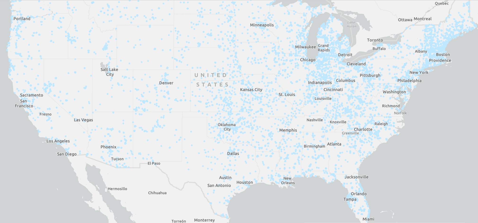
Figure 1: ACRES brownfield locations provided by EPA.

2.1 Socioeconomic Characteristics

We extracted nuclear restrictions in each statesidering it is an uncontrollable parameter for a stakeholder, we define a moratorium as a deal breaker. We express all other restrictions in a single variable as the number of nuclear restrictions in the state. These five remaining restrictions are state legislature approval, state commissioner of environmental protection approval, proving that the construction of a nuclear facility will be economically feasible for ratepayers, demonstrable technology or a means for high-level waste disposal or reprocessing, and proving that the radioactive waste material disposal method will be safe.

We define state electricity price as the annual average electricity price in cents/kWh and electricity imports as the annual amount of electrical power imported by the state in millions of kWh. Our ”population sentiment towards nuclear energy” parameter is an average of the 10-year poll findings of sentiment values of the counties in any 20-mile radius We set state nuclear inclusive policy as a binary value that shows if the state administration has any decisions to support the development of nuclear energy, such as Renewable Portfolio Standards (RPSs), Renewable Portfolio Goals (RPGs), and Clean Energy Standards (CESs).

In energy market regulation, traditional regulation is considered a positive attribute since a regulation authority would help nuclear energy to become the stable baseline in a grid. The construction labor rate is the 5-year average of state labor rate, provided by Occupational Employment and Wage Statistics, in USD.

2.2 Safety Characteristics

We selected safety objectives characteristics that support siting a 1000MWt or higher power reactor [19]. Most of the safety objectives (1, 3, 4, 6, 7) are intersections with dangerous areas explained in the list of objectives provided earlier in this section. NRC Regulatory Guide 4.7, “General Site Suitability Criteria for Nuclear Power Stations” describes that siting nuclear reactors close to the publicly used lands depends on local jurisdictions and can be refused. For this reason, the protected land objective checks if the site intersects with American Indian reservations, correctional facilities, critical habitats, forests, hospitals, national monuments, national or state parks, schools or colleges, wild and scenic rivers, wilderness areas, or wildlife refuges. If the site intersects with any of these, the number of intersections is given.

The objective of “having a near hazardous facility within a 5-mile radius” checks for any petroleum or gas processing facility, pumping stations, fertilizer plants, chemical plants, nuclear fuel plants, storage tanks, and airports. For the fault lines, 10 CFR 100, Appendix A, Table 1 specifies that fault lines within 200 miles of the site must be considered [25]. The STAND tool checks if the location is within 200 miles of any fault line. The United States Geological Survey (U.S.GS) reports the lands that have a moderate or high risk of landslides. This objective states whether the location intersects with a high or moderate landslide-risk area, if any. The peak ground acceleration objective checks for any ground acceleration history higher than 0.3g in the area, which is the suggested limit for the high-power light water reactor (LWR) installations in the 2002 EPRI (Electric Power Research Institute) siting guidance [26].

The flood zone objective checks if the site lies in a 100-year floodplain. For the open waters and wetlands, depending on the region of the open water, these areas are protected by (1) the Rivers and Harbors Act, (2) the Wild and Scenic Rivers Act, (3) the Clean Water Act, (4) the Coastal Management Act, (5) the Coastal Barriers Resources Act, (6) the Fish and Wildlife Coordination Act, (7) the Migratory Bird Conservation Act, and (8) the National Wildlife Refuge Act. This objective checks if the site intersects with lakes, rivers, streams, ponds, etc. The objective featuring the slope of the site is a binary variable that returns 1 if the slope of the site location is higher than 12% as recommended in the 2002 EPRI siting guidance [26].

2.3 Proximity Characteristics

Proximity objectives have been used as binary values as suggested by the STAND tool and previous research conducted in the area. For example, the 10 CFR 100 Regulatory Guide of the U.S. Nuclear Regulatory Commission (NRC) shows that at least a four-mile distance is required between the NPP and the population centers with 25,000 residents [27, 28]. In the STAND tool, this objective is set to 0 if the closest population center distance is closer than four miles. For centers with more than four miles, the objective is linearly scaled between [0,1], where the center with the highest distance from the plant is set to 1.

Communities with existing nuclear technology are generally more supportive of nuclear technology as NPPs are an important source of local jobs and tax revenues. Operating nuclear facilities show the number of nuclear facilities or generators within a 100-mile radius. Having access to nearby nuclear R&D facilities can provide technical support during the development of a nuclear facility. The R&D center objective shows if there is a nuclear R&D center within 100 miles.

The retiring power station objective shows if any coal, natural gas, or nuclear power station is in a one-mile radius in the next 20 years. For the sites with a retiring power station nearby, the distances are linearly scaled to the [0,1] range where the lowest-distance site is set to 1. The substation distance objective is the site distance to the closest electricity grid substation in miles, scaled to [0,1] range where the closest site to the substation is set to 1. We define transportation systems as major roads in the U.S.. The objective is set to 1 if there is a major road closer than 1 mile. For the sites that do not have a major road in a 1-mile radius, the values are linearly scaled to the [0,1] range where the lowest-distance site is set to 1. The streamflow objective shows if there are any freshwater supplies in 20-mile radius, with the minimum 50,000 gallons per minute (GPM) streamflow as recommended in the STAND tool.

The distance values in this section are the distance values that the STAND tool uses for thresholding and linearly scaling the attributes of the selected sites. We selected the generator retirement time (20 years), transportation method (major roads), and streamflow GPM value (50K) with the guidance of the STAND tool developers.

Lastly, an example of the created preprocessed dataset is given in Figure 1. Since the dataset is scaled, higher values for each attribute indicate favorable objectives. For example, 0.9 in the electricity price column indicates a low electricity price in the state, while 0.1 indicates a high electricity price.

Table 1: Preprocessed data with three examples for brownfield sites.

Attribute	Site A	Site B	Site C
Registry ID	110000339982	110000344832	110000346028
Longitude	-76.56465	-81.45892	-80.25551
Latitude	39.27712	39.40018	35.82021
County FIPS	24510	54107	37057
State FIPS	24	54	37
Number of Nuclear Restrictions in the State	0	0	0
State Electricity Price	14.30538462	10.26	10.62692308
State Net Electricity Imports	25934	-28050	14875
State Nuclear Inclusive Policy	0	0	0
Population Sentiment Towards Nuclear Energy	0.402230895	0.428866209	0.658312001
Traditional Regulation In The Energy Market	1	1	1
5-Year Average Labor Rate	34766	35606	30384
Social Vulnerability Index	0.41585454	0.38254449	0.433715808
Number of Intersecting Protected Lands	0	1	0
Number of Hazardous Facilities in 5 Miles	8	6	3
No Fault Line Intersection	1	1	1
No Landslide Area	0	0	0
Having A Peak Ground Acceleration Lower Than 0.3g	1	1	1
Not Having A Flood in Previous 100 Years	0	0	1
No Open Water Or Wetland Intersection	1	1	1
Having A Slope Lower Than 12 Percent	1	1	1
Population Center Distance	3.204225645	13.69500274	13.22706011
Retiring Facility Distance	2.951268247	76.8295757	52.97458529
Existing Nuclear R&D Center in 100 Miles	1	0	1
Electricity Substation Distance	1.381065329	1.642955799	1.266471271
Transportation System Distance	0.778196965	1.49198691	1.235386683
Having A Streamflow with 50 Kgpm Flow in 20 Miles	1	1	1

2.4 Coal Power Plant Sites

According to the U.S. Department of Energy, there are currently 157 inactive and 237 active candidate coal power plant locations that are suitable for housing NPPs [10]. These sites are accompanied by pertinent data, including the 22 objectives outlined in the STAND framework, which are detailed in previous sections and in Table 1. However, the CPP dataset lacks the state federal information processing standard (FIPS) number and county FIPS number from its input data. Previous research identified 265 U.S. coal power plant sites as relevant for NPP siting [19]. Additionally, the coal-to-nuclear transition dataset was updated in October 2024 by the Fastest Path to Zero Initiative (FPTZ) Initiative at the University of Michigan. We have adapted the coal power plant dataset, which was previously examined using the weighted sum method, for multi-objective optimization. By using this dataset, we facilitated a one-to-one comparative analysis with the brownfield sites.

The coal-to-nuclear siting dataset is considerably smaller than the brownfield siting dataset, resulting in significantly shorter processing times. Unfortunately, the limited size also restricts the ability to train machine learning models. Consequently, we exclusively used the brownfield dataset to train the machine learning models. The CPP locations were processed separately, allowing for a comparison between the optimal locations identified in both datasets.

3 Research Methodology

This section describes the methodology used for the assessment of the brownfield and Coal sites described in Section 2, which consists of two major parts. First, we describe our high-dimensional non-dominated combinatorial search approach that is used to rank all sites based on how many times they show up in the Pareto-front when considering every possible combination of the 22 site objectives. This search leads to a set of metrics that describe the importance of each objective to the rank of the site and a site score for global ranking. The site score depends on the dataset used in the analysis. For this reason, the method is repeated for the brownfield sites, CPPs, and a joint dataset of 250 best brownfields and all CPPs. Given our relatively large dataset of more than +30,000 sites, in the second part, we train a data-driven methodology using Concatenated Neural Networks (ConcNN) that allows predicting the (1) site score, (2) site objectives, and (3) importance value of each objective to the site score. The network needs only the site coordinates and location to make such a prediction.

3.1 Non-Dominated, Multi-Objective Combinatorial Search

We used a combinatorial search between the 22 objectives to establish a ground-truth outcome through the application of a non-dominated sorting method. When we perform non-dominated sorting across all objectives at once, the resulting Pareto front comprises 1,294 locations, which yields inconclusive results for a single optimal site. To address this limitation, we applied non-dominated sorting to all possible combinations of objectives. A detailed explanation of these combinations is provided in Table 2, which outlines the combinations of objectives for each specified combination length.

Table 2: Explanation of combination lengths and total number of combinations.

Comb. Length	Combination Examples	Total Number
1	(1), (2), (3), …, (21), (22)	22
2	(1,2), (1,3), (1,4), …, (21,20), (21,22)	231
3	(1,2,3), (1,2,4), (1,2,5), …, (20,21,19), (20,21,22)	1540
21	(1,2, …, 20,21), (1,2, …, 20,22), …, (2,3, …, 21,22)	22
22	(1,2,3, …, 20,21,22)	1

The preprocessed brownfield site objective dataset contains 15,979 rows that represent the individual sites and 22 columns corresponding to objectives. The contiguous U.S. ACRES brownfield dataset includes sites that are often adjacent or in close proximity to one another. Data in the STAND tool rely on state-level and county-level information, proximity to other sites of interest, and integration with geographical databases. We expect locations within close proximity to exhibit identical characteristics. To manage this redundancy, we truncated site coordinates to 0.01 degrees of longitude and latitude, and we removed sites with identical truncated coordinates from the dataset. Later, we inferred the siting results for these removed locations by using results from persisting locations with the same truncated coordinates. This method introduces an uncertainty of approximately 0.315 miles in the southern U.S. and 0.246 miles in the northern U.S. due to the truncation of coordinates. The computational complexity of the non-dominated sorting method varies between $O(N\log N)$ and $O(N^{2})$, depending on the implementation and problem structure. Reducing the number of sites from 34,212 to 15,979 results in a 56.34% decrease in computation time under the low-complexity $O(N\log N)$ scenario and a 77.85% decrease under the high-complexity $O(N^{2})$ scenario.

The non-dominated, multi-objective combinatorial search starts from combination length $s=1$. We only apply non-dominated sorting a single selected objective at a time. For the combination length $s=1$, we apply non-dominated sorting $k\in[1,22]$ times for the examples given in Table 2.

The preprocessed 15,979 rows of data is defined as the matrix $\widehat{A}$ where $\widehat{A}\in\mathbb{R}^{15979\times 22}$. The subsets of $\widehat{A}$ that only include selected column indices are defined as $\widehat{A}_{L_{k}}$, i.e. $\widehat{A}_{L_{k}}\in\widehat{A}$.

We generated the possible combinations of the siting objectives using $C(s,t)$. For $C(1,22)$, there are 22 different $C_{k}$ elements to select, each of these elements is given in Table 2. This operation creates $L$, the possible combinations that choose $s$ elements from a set of $t$ elements regardless of order. $L_{k}$ defines a single combination in the list $L$.

$$\begin{split}C(s,22)=L\\ L=\{L_{1},L_{2},L_{3},\ldots,L_{k}\}\\ \end{split}$$ (1)

Note that $L$ depends on $s$. For simplicity, we omit the subscript $s$ in the notation for $L$ and the vectors up to $\overrightarrow{SR}$ as discussed in this section.

The function $NS$ is defined as the operation that applies non-dominated sorting on a matrix. The $NS$ function outputs a column vector $\overrightarrow{r}_{k}$ with 15,979 rows indicating the domination for each site. $\overrightarrow{r}_{k}$ has 1 in the ”dominating” $\widehat{A}$ site indices and 0 in the “dominated” site indices. For each $\widehat{A_{L_{k}}}$ subset, there is an unique $\overrightarrow{r}_{k}$ vector.

$$NS(\widehat{A}_{L_{k}})=\overrightarrow{r}_{k},\quad\overrightarrow{r}_{k}\in\mathbb{R}^{15979\times 1}$$ (2)

The next step involves the summation and normalization of each vector $\overrightarrow{r}_{k}$, resulting in the normalized observation ratio $\overrightarrow{NR}$. Summing the normalized observation ratios across various combination lengths $s$ yields the summed normalized observation ratio $\overrightarrow{SR}$. Finally, applying min-max scaling to $\overrightarrow{SR}$ within the range $[0,1]$ produces $\overrightarrow{\mathbb{M}}$, which acts as a site performance metric for selecting the most suitable reactor sites.

$$\begin{split}\overrightarrow{\text{NR}}=\frac{\sum_{k}\overrightarrow{r}_{k}}{\left|\sum_{k}\overrightarrow{r}_{k}\right|}\\ \widehat{SR}=\sum_{s=1}^{22}\widehat{NR}\\ \overrightarrow{\mathbb{M}}=\frac{\overrightarrow{SR}-\min(\overrightarrow{SR})}{\max(\overrightarrow{SR})-\min(\overrightarrow{SR})}\end{split}$$ (3)

The methodology presented is based on the non-dominated sorting approach, which we employed to identify the optimal individuals within a given set. Consequently, the siting metric derived from this method is inherently influenced by the specific sites included in the dataset. We demonstrate an example of aquiring the site observation ratio below. In this problem, we select the 3-length combination of the objectives.

$$C(3,22) =L=[L_{1},L_{2},L_{3},\ldots,L_{1540}]$$

$$L_{230} =\begin{bmatrix}2,3,5\end{bmatrix}$$

The function $C(s,t)$ creates the list of the combinations. We select the $230^{th}$ item on this listfor demonstration. This lis, $L_{230}$, includes the column (objective) numbers 2, 3, and 5, which represent state electricity price, state electricity imports, and population SVI, respectively. The subset $L_{230}$ of the dataset $\widehat{A}$ shown below:

$$\widehat{A}_{L_{230}} =\begin{bmatrix}0.2023&0.6605&0.6158\\ 0.0729&0.2907&0.5883\\ 0.3935&0.5107&0.9067\\ 0.4777&0.7118&0.6409\\ \vdots&\vdots&\vdots\end{bmatrix}$$

Applying non-dominated sorting to the dataset subset creates $\overrightarrow{r}_{230}$ as follows:

$$NS(\widehat{A}_{L_{230}}) =\overrightarrow{r}_{230}=\begin{bmatrix}0\\ 0\\ 1\\ 1\\ \vdots\end{bmatrix}$$

This vector indicates that the sites at the first and second row indices are dominated by the other sites in this example. After finding the domination status of all locations for all 3-length combinations of the siting objectives (from 1 to 1,540 total combinations), we normalize the summed vector:

$$\overrightarrow{NR} =\begin{bmatrix}0\\ 0\\ 0.0002\\ 0.0002\\ \vdots\end{bmatrix}$$

Summing $\overrightarrow{NR}$ for all combination lengths creates the summed normalized observation ratio $\overrightarrow{SR}$, which can then be converted by min-max normalization to $\overrightarrow{\mathbb{M}}$ (the siting metric) as follows:

$$\overrightarrow{SR} =\begin{bmatrix}0.013\\ 0.008\\ 0.029\\ 0.034\\ \vdots\end{bmatrix}$$

$$\overrightarrow{\mathbb{M}} =\begin{bmatrix}0.0065\\ 0.0040\\ 0.0145\\ 0.0170\\ \vdots\end{bmatrix}$$

Following the site score, $\overrightarrow{\mathbb{M}}$, we seek to determine which of the 22 objectives contribute the most to the site score. This provides a more informative explanation for a given site’s suitability. To do this, we start by defining the summed normalized objective contributions ($\widehat{SC}$), which show the contribution of each objective to a specific site performance. Then, the dominating indices vector $\overrightarrow{r}_{k}$ is multiplied with $\overrightarrow{v}_{k}^{T}$. The column vector $\overrightarrow{v}_{k}$ shows which objectives are included in the current combination:

$$\begin{split}\overrightarrow{v}_{k}[i]=\begin{cases}1&\text{if }i\in L_{k}\\ 0&\text{if }i\notin L_{k}\end{cases}\\ \widehat{R}_{k}=\overrightarrow{r}_{k}\cdot\overrightarrow{v}_{k}^{T}\end{split}$$ (4)

Note that $\overrightarrow{v}_{k}$ depends on $s$. For simplicity, the subscript $s$ is omitted in the notation for $\overrightarrow{v}_{k}$ and the matrices up to $\widehat{S}$ as discussed in this section.

The vector $\overrightarrow{v}_{k}$ has 1 at the indices included in the objective combination $L_{k}$ for the combination $k$. The matrix $\widehat{R}_{k}$ resulting from the dot product shows which objectives (column indices) affected the performance of the sites (row indices). We define $\widehat{R}_{k}$ as the contribution matrix for the $k^{th}$ objective combination in the dataset. These contribution matrices are summed for different combinations within the same combination length as follows:

$$\widehat{OC}=\sum_{k}\widehat{R}_{k}$$

The objective contribution ($\widehat{OC}$) is row-normalized to not favor any combination length. The indices $i$ and $j$ represent the row and column indices of the matrix, respectively, and are normalized such that the sum of each row equals 1.

$$\widehat{NC}_{i,j}=\frac{\widehat{OC}_{i,j}}{\sum_{j}\widehat{OC}_{i,j}}$$

The normalized objective contributions ($\widehat{NC}$) are then summed for all combination lengths to get the summed objective contribution ($\widehat{S}$).

$$\begin{split}\widehat{S}=\sum_{s=1}^{22}\widehat{NC}\\ \end{split}$$

The summed objective contribution ($\widehat{S}$) matrix is row normalized to set the sum of importance to 1 for every site individually in the dataset. The aforementioned operations form the normalized summed objective contribution ($\widehat{SC}$).

$$\begin{split}\widehat{SC}_{i,j}=\frac{\widehat{S}_{i,j}}{\sum_{j}\widehat{S}_{i,j}}\end{split}$$

An example of achieving the normalized objective contributions is given below. For the selected same objective combination (k=230) with the column numbers 2, 3 and 5, the non-dominated sorting result is given as $\overrightarrow{r}_{230}$. Each row shows a site index which dominates the result of the non-dominated sorting.

$$\begin{split}\overrightarrow{r}_{230}&=\begin{bmatrix}0\\ 0\\ 1\\ 1\\ \vdots\end{bmatrix}\\[10.00002pt] \end{split}$$

The combination selected for this example includes the columns 2, 3 and 5 of the dataset. The subset including these columns is given as $L_{230}$.

$$\begin{split}L_{230}&=\begin{bmatrix}2,3,5\end{bmatrix}\\[10.00002pt] \end{split}$$

We use the combination of objectives in this example to create a vector where an entry is 1 if the corresponding objective index is included and 0 otherwise. Note that the length of the vector $\overrightarrow{v_{230}}$ is 22, but only the indices 2, 3, and 5 are non-zero.

$$\begin{split}\overrightarrow{v}_{230}&=\begin{bmatrix}0\\ 1\\ 1\\ 0\\ 1\\ \vdots\end{bmatrix}\\[10.00002pt] \end{split}$$

The matrix $\overrightarrow{R_{230}}$ is created from the dot product of $\overrightarrow{r}_{230}$ and $\overrightarrow{v}_{230}^{T}$.

$$\begin{split}\widehat{R}_{230}&=\begin{bmatrix}0&0&0&0&0&\ldots\\ 0&0&0&0&0&\ldots\\ 0&1&0&1&1&\ldots\\ 0&1&0&1&1&\ldots\\ \vdots&\vdots&\vdots&\vdots&\vdots\end{bmatrix}\\[10.00002pt] \end{split}$$

The contribution matrices of combinations $R_{k}$ are summed for all existing combinations of the given combination length ($s=3$).

$$\begin{split}\widehat{OC}&=\begin{bmatrix}0.3&0.5&2&0.7&0.1&\ldots\\ 5&1.1&0.6&0.1&0.3&\ldots\\ 0.2&1.2&0.3&1.7&1&\ldots\\ 0.1&0.2&0.1&1.3&0.5&\ldots\\ \vdots&\vdots&\vdots&\vdots&\vdots\end{bmatrix}\\[10.00002pt] \end{split}$$

The objective contribution matrix of the combination length ($s=3$) is normalized to create the normalized objective contribution matrix $\widehat{NC}$.

$$\begin{split}\widehat{NC}&=\begin{bmatrix}0.08&0.14&056&0.19&0.03&\ldots\\ 0.70&0.15&0.08&0.01&0.04&\ldots\\ 0.05&0.27&0.07&0.39&0.23&\ldots\\ 0.05&0.10&0.05&0.55&0.10&\ldots\\ \vdots&\vdots&\vdots&\vdots&\vdots\end{bmatrix}\end{split}$$

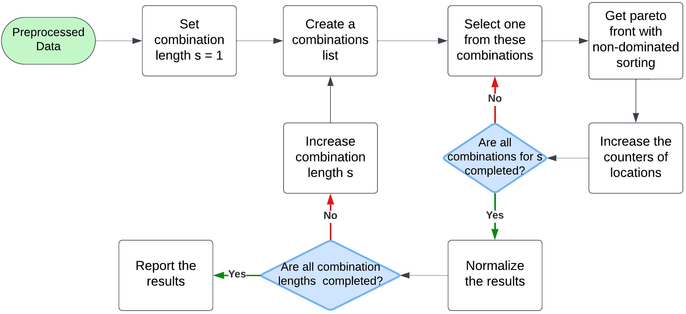
Figure 2: A multi-objective analysis combinatorial analysis for nuclear reactor sites.

We summarize this method in the flowchart shown in Figure 2. The application of the prescribed method presented several challenges, primarily due to the rapid increase in the number of combinations with varying combination lengths. Prior to the analysis, we executed the siting analysis routine computer core counts and combination lengths. Based on the scaling for core numbers, we anticipated that the complete analysis of all combination lengths would require approximately 8.5 days running on 512 cores. To mitigate the risk of processes being forcibly terminated due to extended runtimes and to address program memory issues, we implemented a checkpoint system between each combination length. We then executed the method in segments, each lasting approximately three days. Each checkpoint records the elapsed computation time for each combination length and the data processed up to that point. We provide a comparison of combination lengths and their corresponding computation times in Table 3.

Table 3: Computation times for different combination lengths

Combination Length	1	2	3	4	5	6	7	8	9
Computation Time (min)	0.028	0.29	2.01	11	43.94	134.85	250.65	408.96	937.46

3.2 Concatenated Neural Networks (ConcNN)

To evaluate the impact of each parameter on various locations, we propose a Feed-Forward Neural Network (FNN) model. This model aims to predict the siting metric and the importance of site objectives for any location within the contiguous U.S.. Additionally, it seeks to identify which objectives will influence siting decisions, eliminating the need to re-run the high-cost analysis described in the previous section.

The FNN model is composed of two parts. The first part of the model uses the longitude, latitude, county FIPS code (Federal Information Processing Standards), and state FIPS code as its input and the 22 site objectives as the output. The model predicts the siting objectives for a given location by interpolating between the existing locations in the dataset. These predicted objectives are then passed to the second stage of the model. In this stage, the 22 objective predictions, along with the original coordinates, county FIPS, and state FIPS, are input to predict the siting metric (score) and the objective importance values.

To develop the described model, we defined our input data ($X$) with four features, including coordinates, state, and county information. This input passes through a series of hidden layers, producing an intermediate output ($Y_{1}$) that predicts two sets of variables: 14 continuous variables ($Y_{L}$) and 8 binary variables ($Y_{B}$). These variables represent the siting objectives, derived from the STAND tool that are relevant to the chosen location. The intermediate output ($Y_{1}$) is then concatenated with the initial input data ($X$), forming an enhanced feature set. The model then processes this concatenated data through subsequent hidden layers to predict additional siting metrics and objective importance scores ($Y_{2}$). We then train the model to optimize predictions for both $Y_{1}$ and $Y_{2}$ simultaneously. This improved model performance compared to a standard FNN since the initial part of the model is further refined using outputs from the second part.

We conducted hyperparameter tuning using grid search for each of the following parameters: the number of hidden layers of the first part (ranging from 1 to 8), the number of hidden layers of the second part (ranging from 1 to 8), the number of neurons per layer (between 25 and 1,000), and the learning rate (between 1e-5 and 1e-3). The flowchart illustrating the data flow of the model is presented in Figure 3.

To speed up the calculations, we explored an alternative method to replace the first stage of the ConcNN model. This alternative uses a lookup table combined with a linear interpolation scheme to predict NPP siting objectives across locations in the contiguous U.S.. In the original ConcNN model, the first stage processes four input parameters to predict 22 siting objectives. For predicting the characteristics of the locations, the lookup table and interpolation method are expected to perform effectively. This is because most siting objectives are primarily influenced by proximity-based metrics. LUT-NN refers to this revised model, which uses a lookup table for predicting the site objectives. ConcNN will be used to refer to the original, fully neural network model that predicts all outputs.. Later in the results section, we benchmark both LUT-NN and ConcNN in predicting site objectives, the siting metric, and objective importance values. The data flow for both LUT-NN and ConcNN models is given in Figure 3 and 4.

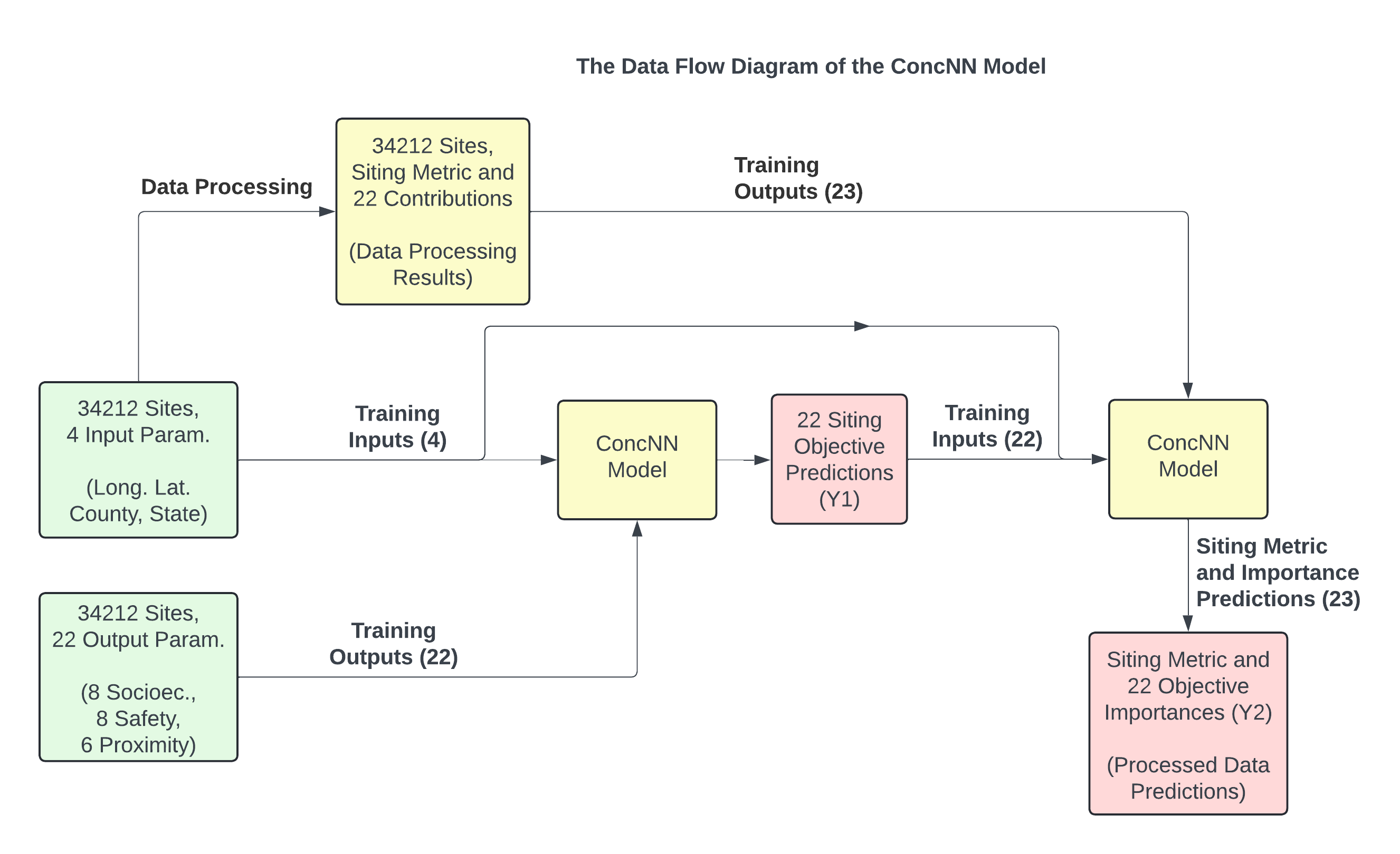
Figure 3: Visualization of the data flow of the ConcNN model (concatenated neural network).

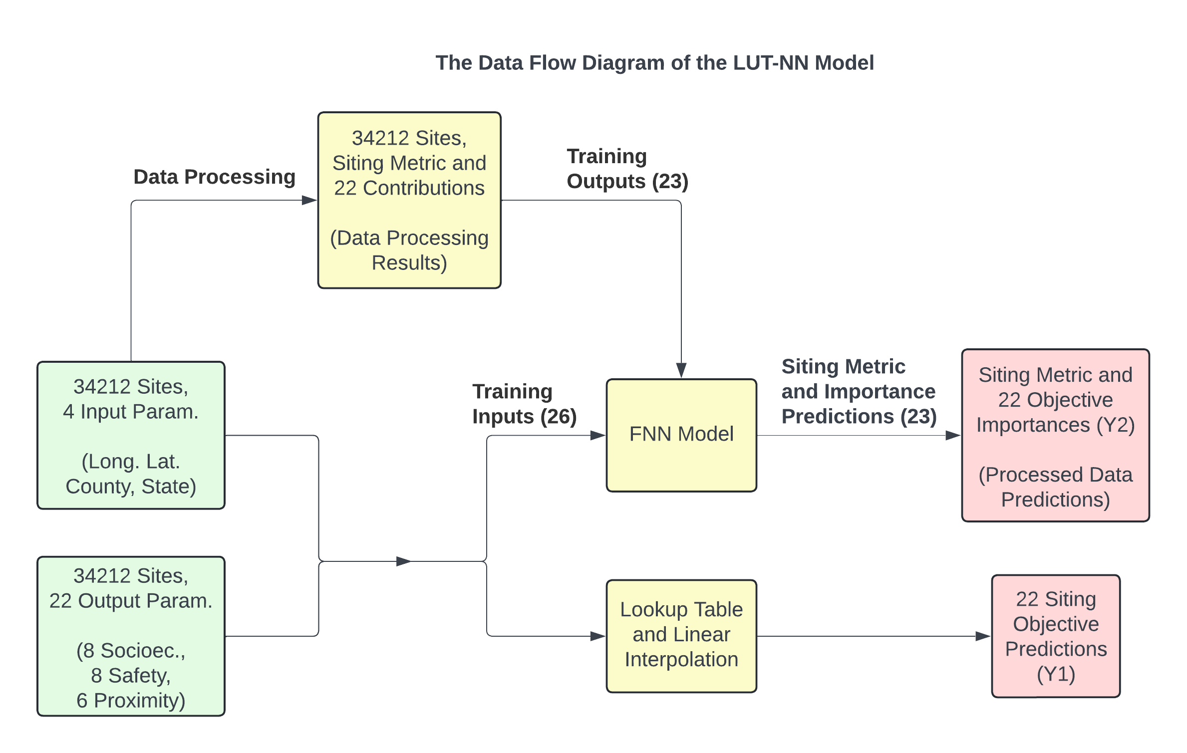
Figure 4: Visualization of the data flow of the LUT-NN model (lookup table plus neural network).

3.3 Computing Resources

This study used the Idaho National Laboratory High-Performance Computing (INL-HPC) system to conduct the one-time combinatorial search described in Section 3.1. The analysis encompassed all brownfield sites, CPP sites, and the combined dataset of brownfield and CPP sites. The computations were performed in parallel on the Bitterroot cluster, utilizing 512 cores. Each CPU in the cluster is an Intel® Xeon® Platinum 8480+ with 56 cores operating at a frequency of 3.8 GHz, with 256 GB of RAM per node. The search was successfully completed over a span of nine days.

For the machine learning training, we employed TensorFlow 2.18.0 and Keras 3.6.0 to develop and train the ConcNN model, as detailed in Section 3.2. We conducted the training and hyperparameter tuning on an internal GPU server at the University of Michigan. This server is equipped with two AMD EPYC 9654 processors, each providing 96 cores operating at 2.4–3.7 GHz, resulting in a total of 192 cores and 384 threads. Additionally, the server features four NVIDIA RTX 6000 Ada Generation GPUs and 1536 GB of DDR5 RAM. The training and tuning process completed in approximately 18 hours.

4 Results and Discussions

4.1 Reactor Siting Analysis in the United States

We analyzed the brownfield location dataset using the resources explained in Section 3.3 until site observation ratios for all 22 combination lengths were computed based on the method presented in Section 3.1. After this process, we used the resulting data to calculate the siting metric. We used this siting metric to identify optimal locations and evaluate the influence of each objective on the site score. The workflow employed to derive these findings is summarized in Figure 5.

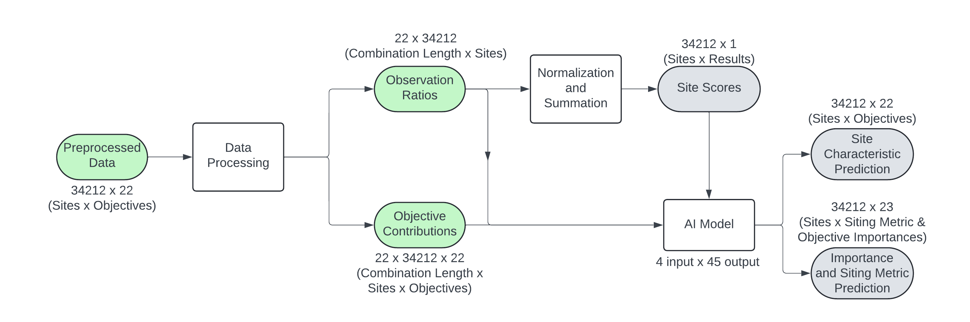
Figure 5: A flowchart summarizing the results acquired from brownfield sites dataset.

To illustrate how the processed data varies with changing combination lengths, we plot the site observation ratios for different combination lengths prior to summing them. The top-performing locations and their observation ratios across various combination lengths are presented in Figure 6.

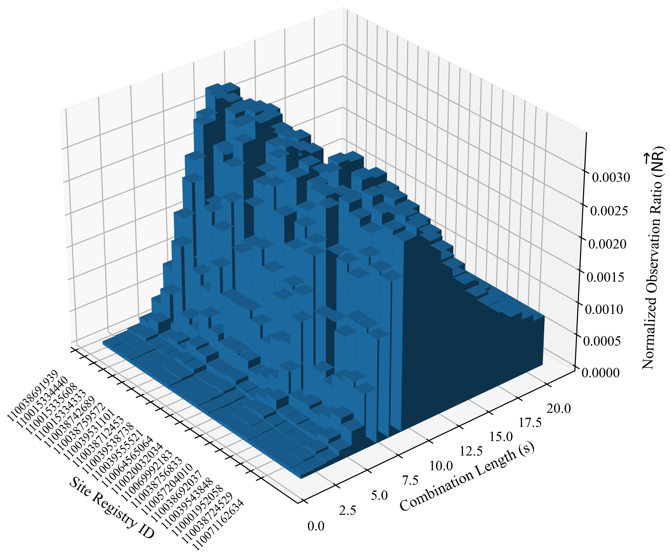
Figure 6: The normalized observation ratio as a function of combination length from the non-dominated multi-objective combinatorial search. The plot shows the change of $\overrightarrow{NR}$ with combination length ($s$) for the top performing 20 brownfield sites.

Considering the required computational power, we present the non-dominated, multi-objective combinatorial search operation as a brute-force method for this dataset. The number of locations is significantly larger in the brownfield siting dataset (34,212) than the coal site dataset (265). For this reason, non-dominated, multi-objective combinatorial search provides more reliable outcomes on the brownfield NPP siting dataset. We give the product of these operations as a summed and scaled observation ratio (siting metric) for each location. The site scores of the best brownfield sites are given in Table 4.

Table 4: Site scores (summed and scaled observation ratios $\overrightarrow{\mathbb{M}}$) by site ID, state and county for the top five performing brownfield locations in the contiguous U.S..

Brownfield ID	State	County	Longitude	Latitude	Siting Metric ($\overrightarrow{\mathbb{M}}$)
110038759572	FL	St. Lucie	-80.320	27.418	1.000
110015334440	CA	Almeda	-122.103	37.668	0.989
110038756833	MT	Garfield	-106.907	47.318	0.988
110039543330	CT	Hartford	-72.674	41.763	0.973
110038712453	NC	Wake	-78.631	35.763	0.945

For the best-performing site ( ACRES location ID 110038759572, which is located in St. Lucie County, Florida), the change in the observation ratio is illustrated in Figure 7. As shown, the observation ratio tends to decrease with increasing combination length. This trend is consistent across all other sites examined in the procedure outlined in Figure 2. We attribute the observed decrease to the total number of combinations associated with different combination lengths; specifically, fewer combinations at both high and low combination lengths (see Table 2) result in lower observation rates. This becomes more obvious in Figure 8, which shows the change in the normalized observation ratio variance as a function of combination length. Nevertheless, high-order combination lengths (e.g. 18-20) cause larger variance in the observation ratio compared to the low-order ones (e.g., 3-5)

We show one of the most interesting findings in this study in Figures 6-8, which reveal that the most promising sites tend to exhibit a prominent observation rate on the Pareto front at higher combination lengths, peaking between 10-12 combinations. This suggests that the interaction between objectives plays a critical role in site ranking. Simply assigning weights to individual objectives fails to capture these high-dimensional interactions. These higher-order interactions significantly influence site ranking, while lower-order combination lengths have a relatively smaller impact on the variance of observation rate for different sites.

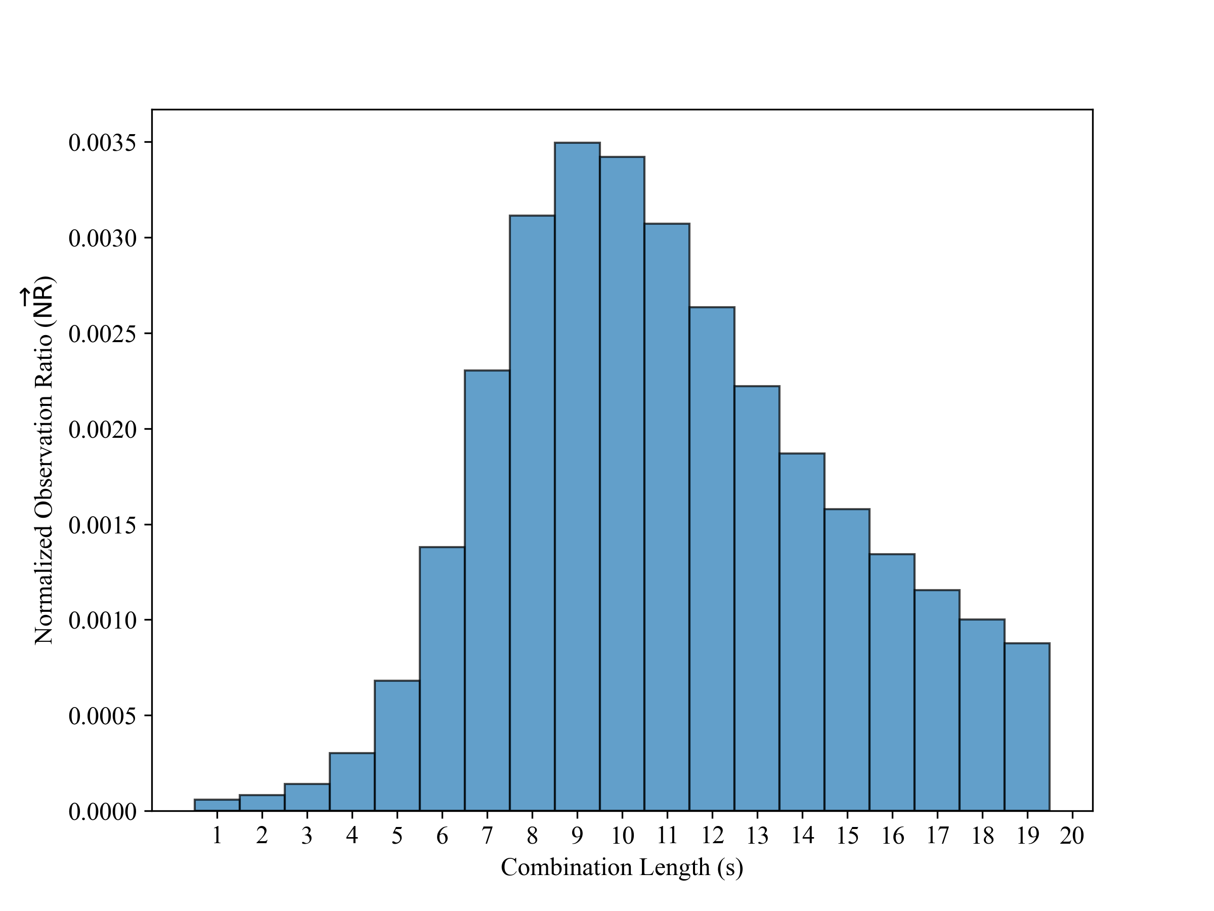
Figure 7: Normalized observation ratio ($\overrightarrow{NR}$) of the best performing brownfield site (ACRES Registry ID 110038759572 in St. Lucie County, Florida) for different combination lengths ($s$).

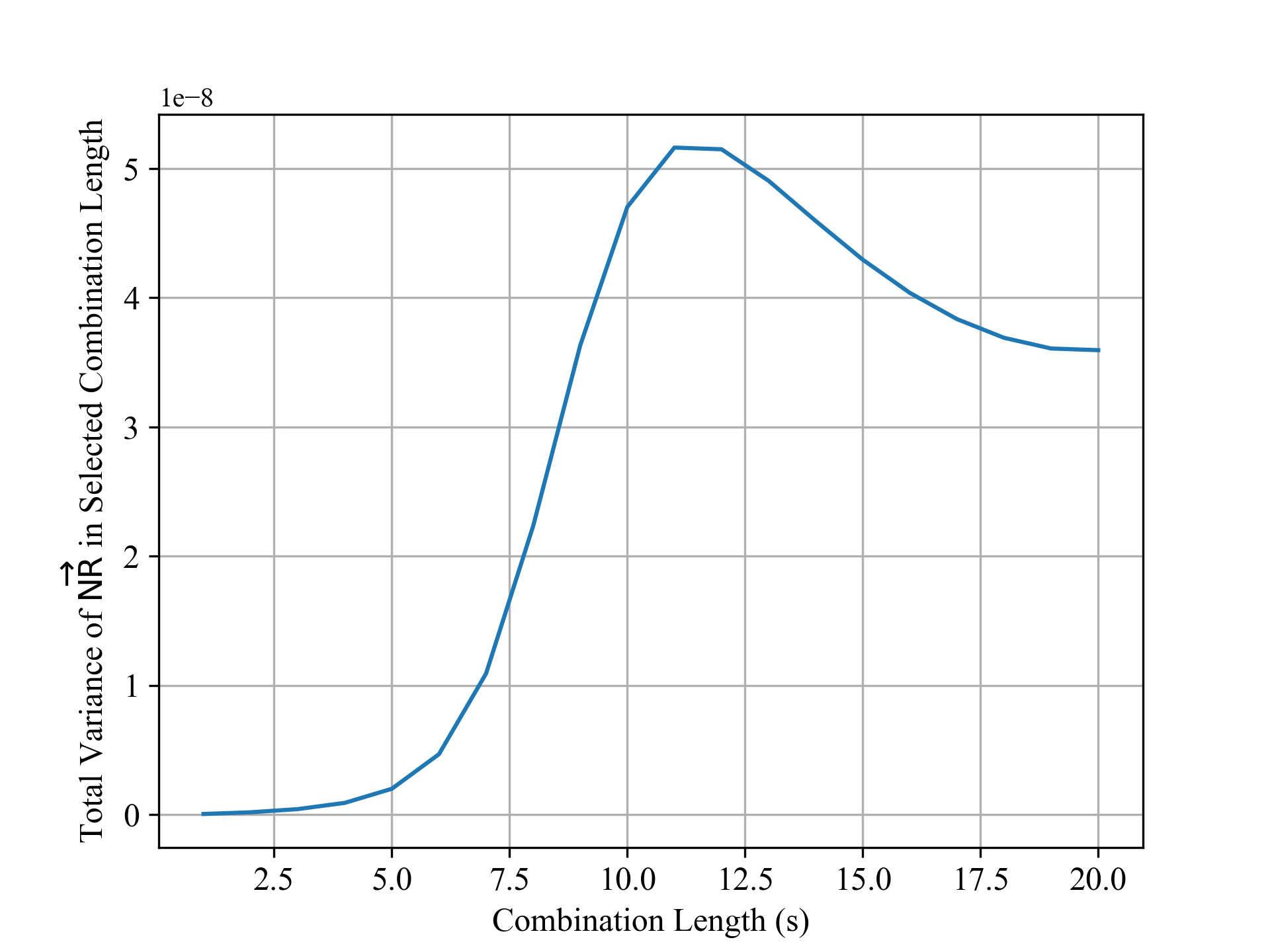
Figure 8: The variance in the normalized observation ratio as a function of the combination length ($s$). This figure shows how the $\overrightarrow{NR}$ results differ for increasing combination lengths. For $s=1$, the rows of $\overrightarrow{NR}$ are mostly the same (for each site) with approximately 0 variance in the vector.

The top-performing brownfield locations identified in this analysis are situated in St. Lucie County, Florida (FL); Alameda County, California (CA); Garfield County, Montana (MT); Hartford County, Connecticut (CT); and Wake County, North Carolina (NC). Key distinguishing objectives for these sites include distance to retiring facilities, public sentiment toward nuclear energy, proximity to nuclear R&D centers, terrain slopes, and fault line proximity. Of these five sites, only the location in California (2) has a nuclear restriction, which is the need for high-level waste disposal technology or reprocessing capacity. In terms of energy policy and incentives, the top two sites in Florida (1) and California (2) have nuclear-inclusive policies, while the third site in Montana (3) has higher electricity prices. Additionally, the California site (2) operates in a traditionally regulated energy market; all other sites have deregulated markets. California, however, it is the only location adjacent to protected lands. From a safety perspective, only the Montana site (3) is within 200 miles of a fault line, but it ranks positively for all other safety objectives because it is the safest site in the top five results. The California site (2) is the only site with multiple nearby nuclear R&D centers. he Florida site (1) ranks highest for population sentiment favoring nuclear energy.

This analysis shows optimal site selection without weighting the importance of specific objectives,thereby yielding an objective conclusion. This is a stark contrast to the subjectivity of status quo methods. The attributes of the top brownfield sites highlight the balanced nature of competing objectives in the selection process.

To create a joint dataset between brownfield and CPP sites, the top 250 sites from the brownfield dataset were combined with all 265 sites from the CPP dataset. A consistent combinatorial methodology was applied to assess and compare optimal brownfield and coal power plant (CPP) sites, facilitating a comprehensive analysis of the top-performing locations across both types of sites. The best 20 sites from this comparison, along with their coordinates and site metrics, are illustrated in Figure 9.

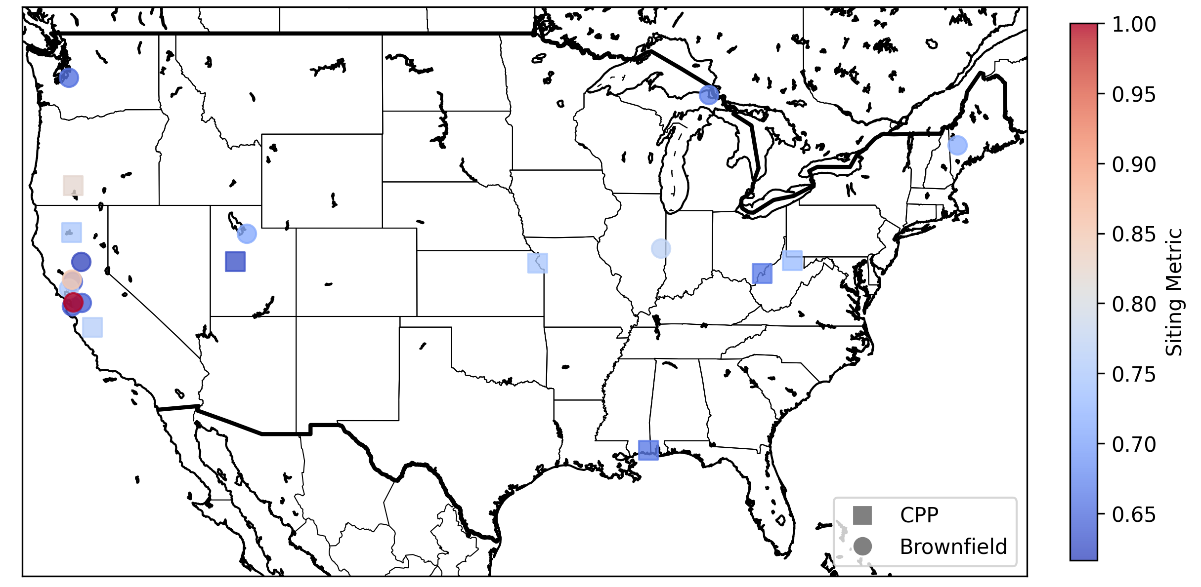
Figure 9: Best performing brownfield and coal sites of the joint dataset based on the non-dominated multi-objective combinatorial search.

The map includes 12 brownfield sites and 8 CPP sites, where each location is based on optimal combinations of the 22 objectives in the joint dataset. The best sites in this comparative study are located in Almeda County in CA, Yolo County in CA, Milwaukee County in WI, Plumas County in CA, Person County in NC. Analysis of objective contributions to the siting metric (score) reveals that each site excels in different dominant objectives impacting its performance. For instance, the model choses Almeda County, California site for its high electricity price, proximity to a significant number of nuclear R&D facilities, and optimal values across other key objectives. Compared to this, the Milwaukee County, Wisconsin site demonstrates stronger safety-related objectives, lower proximity advantages and distant to key objectives, and equivalent economic metrics. This example highlights clear trade-offs between the sites.

The method implemented in this study employs non-dominated sorting to identify the optimal locations. This approach selects locations that are not dominated by others based on the given criteria. The results of the method depend on the dataset used. In the brownfield study, the best site identified was in St. Lucie County, Florida. The objective contributions indicate that this site was selected due to the absence of state nuclear restrictions, the presence of a traditionally regulated energy market, the lack of protected lands, fault lines, landslide hazards, and open water, a peak ground acceleration lower than 0.3g, a slope less than 12 percent, proximity to a substation, and the availability of streamflow.

If a site were to offer at least one superior objective while maintaining the same favorable attributes described above, the St. Lucie County site would be dominated in most combinations. Since the introduction of CPP sites has eliminated St. Lucie County, Florida, as a viable option, we can infer that a CPP site dominates the St. Lucie County site.

The detailed siting metrics and objective values for the top CPP and brownfield sites are provided in Table 8 in the Appendix. The objective importance values of the best brownfield and coal sites in the joint dataset is given in Figure 10.

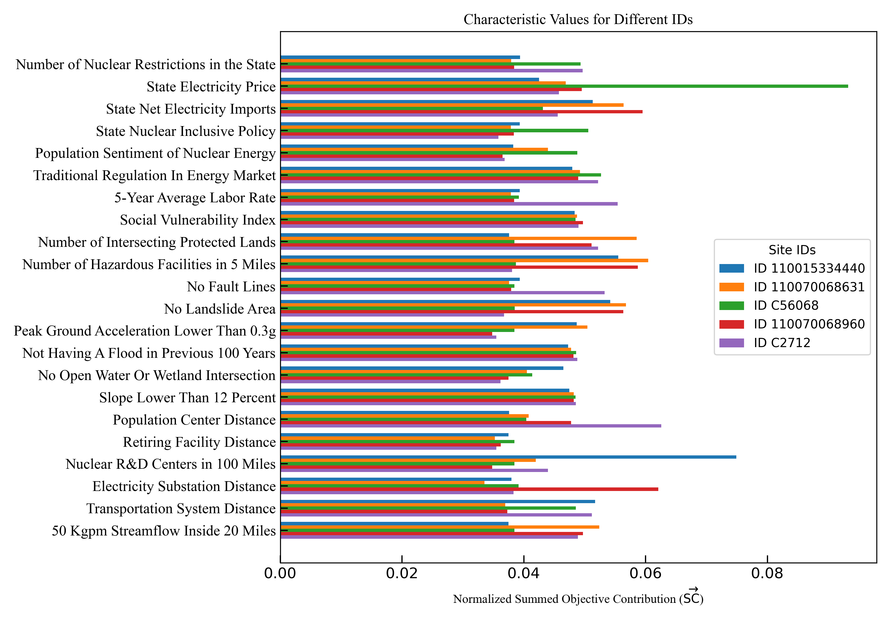
Figure 10: Summed normalized objective contributions ($\overrightarrow{SC}$) of the best-performing locations in the brownfield and coal site joint dataset. Further details about each site are given in Table 8.

Upon examining the results of the joint brownfield and coal sites, we identify the top two performing sites as brownfield locations. In the top 20 sites, the number of brownfields and coal power plant (CPP) locations are close to each other, meaning that both site options are competitive. Notably, the CPP sites predominantly meet safety objectives, as they are generally located away from external hazards. Coal sites are also strategically positioned near electricity substations, streamflow resources, and major roads, providing an advantage in grid connectivity and infrastructure accessibility over brownfield sites. However, the brownfield sites span locations across all contiguous U.S. states. Given the higher number of brownfield sites relative to coal power plants, it is more likely that optimal locations with strong overall objectives can be identified among brownfields instead of CPPs.

Our research methodology employs non-dominated sorting to identify locations that dominate across multiple objectives, without considering the specific magnitude of each objective. This approach prioritizes a location’s relative performance on individual objectives rather than their absolute values. Consequently, even if an objective holds the extreme (best or worst) value in the dataset, its specific magnitude is not factored into the sorting process. For instance, the highest-ranked location has several nearby hazardous facilities, yet it outperforms others due to advantageous factors such as state electricity imports, proximity to retiring facilities, nearby nuclear R&D centers, and distances to both electricity substations and transportation systems. This outcome underscores that certain important objectives in top locations are outweighed by the sheer number of other objectives. This illustrates how trade-offs become inherent to multi-objective optimization.

4.2 ConcNN Model Results

Based on the method presented in Section 3.2 and after collecting an enormous amount of information from our combinatorial search, we built a data-driven model to predict the NPP siting objectives, siting metric, and objective importance values based on the site location.

The model evaluations in this section use Mean Squared Error (MSE), Root Mean Squared Error (RMSE), Mean Absolute Error (MAE), and $R^{2}$ (coefficient of determination). MSE measures the average squared difference between predicted and actual values, penalizing larger errors more heavily. RMSE, the square root of MSE, expresses the error in the same units as the target variable, making it more interpretable. MAE calculates the average absolute differences, providing a more direct measure of typical error without emphasizing outliers. $R^{2}$ evaluates the proportion of variance in the target variable explained by the model, with values closer to 1 indicating better fit. We report these metrics in tables for the evaluated models.

The best ConcNN model after tuning consists of six layers of 1000 neurons in its first part, and two layers of 400 neurons in its second part. We set the learning rate to 1e-3. We select the test data proportion to be 20% of the total dataset (6,842 site locations). The test set is used to assess model performance through site locations not used during training. We set the number of epochs to 1,000 and the batch size to 128. The siting objective prediction ($Y1$) and siting metric and objective importance prediction ($Y2$) training metrics for the ConcNN model are given in Table 5. The model training loss is given in Figure 12. The best ConcNN architecture is sketched in Figure 11.

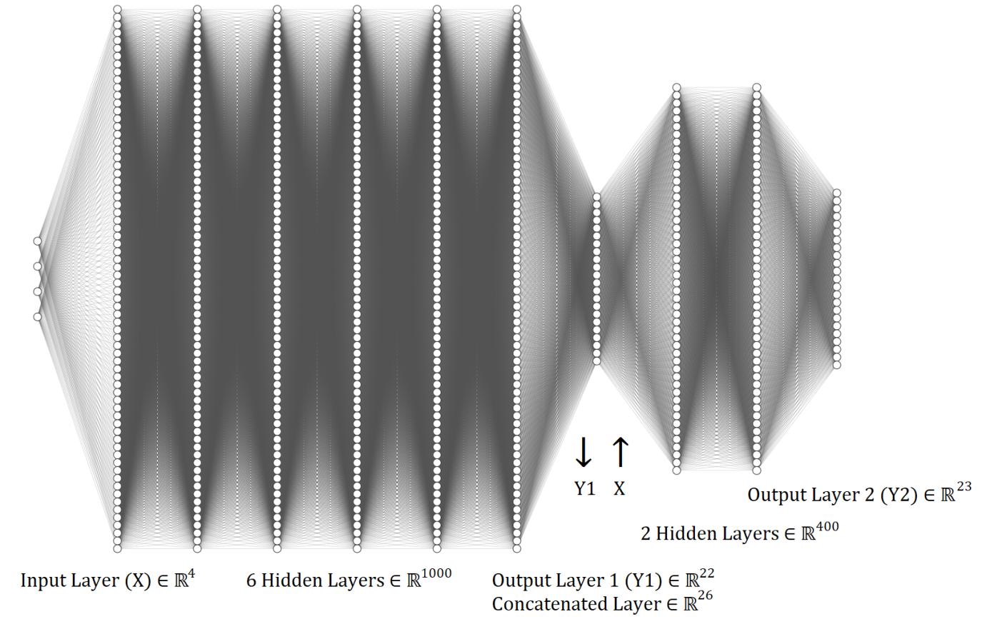
Figure 11: Architecture of the ConcNN model

Table 5: ConcNN Model Training and Test Metrics

Metric	MSE	RMSE	MAE	R²
Y1 Training	5.49058	2.34324	0.55280	0.85176
Y1 Test	7.6995	2.77481	0.58179	0.79706
Y2 Training	0.00018	0.01355	0.00657	0.76858
Y2 Test	0.00023	0.01522	0.00749	0.70403

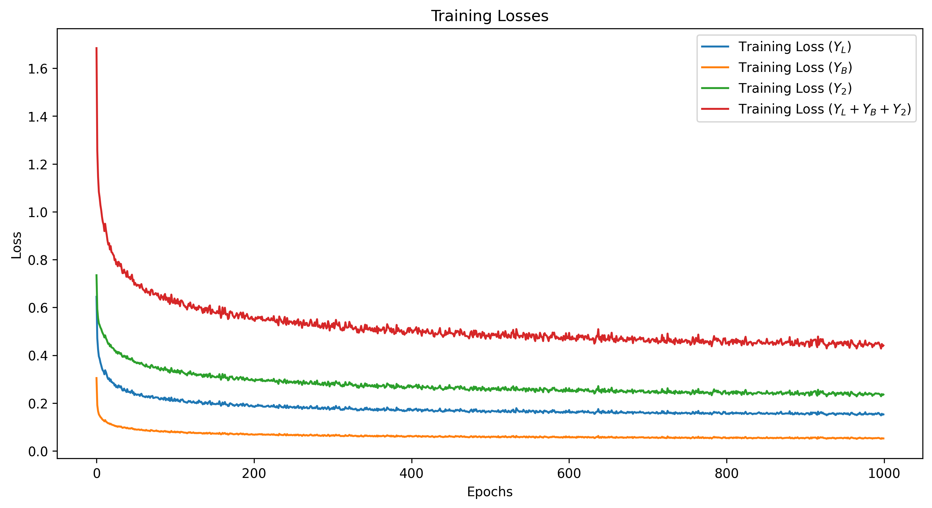
Figure 12: The change of $Y_{L}$, $Y_{B}$, $Y_{2}$ training losses and the total training loss with epoch.

The metric results in Table 5 indicate that while the ConcNN model performs reasonably well, it lacks high accuracy in predicting site characteristics, with an $R^{2}$ on the test set ranging from 0.7 to 0.8 for its two output layers ($Y1$ and $Y2$), compared to the ideal $R^{2}$ of 1.0. This suggests that, despite being trained on a dataset of approximately 34,000 points, the problem remains challenging to model purely by machine learning. The primary difficulty arises because the model receives only four input features related to the site’s location and is tasked with predicting 22 site objectives. As a result, predictions may be particularly error-prone near state borders where site objectives objectives may exhibit significant variability in response to minor changes in input parameters. Furthermore, the lower accuracy in predicting $Y1$ propagates to $Y2$, leading to even lower $R^{2}$ values for the second output. Despite these limitations, the authors believe that the model can still offer rapid predictions of site objectives, site scores, and objective importance values that capture general trends across U.S. sites. However, its errors may be significant enough to limit its utility for precise site ranking.

4.3 LUT-NN Model Results

We present an assessment of LUT-NN, which replaces the first part of ConcNN with a lookup table and linear interpolation, in this section. The hyperparameter tuning for the LUT-NN was conducted over a broad range of values: the number of layers varied from 1 to 10, the number of neurons per layer ranged from 25 to 1,000, and the learning rate was tested between 1e-3 and 1e-5. The optimal model configuration identified consisted of six layers with neuron counts of [750, 750, 750, 700, 700, 650] in each layer, and an initial learning rate of 2e-4. We applied a learning rate decay factor of 0.92 with early stopping patience set to 25 epochs and trained the model for 1,000 epochs with a batch size of 32. To address overfitting, we applied L2 regularization with values ranging from 1e-2 to 1e-5, as well as dropout rates between 0.05 and 0.5, to each layer. Unfortunately, these strategies were not effective in improving prediction accuracy for locations that are absent from the lookup table.

The prediction metrics of LUT-NN for the $Y1$ values are shown in Table 6 for the test sites that exist in the dataset. As expected, the model perfectly predicts test sites. This is represented by the metrics in Table 6. However, to evaluate the $Y1$ metrics with LUT-NN for the site locations that do not exist in the lookup table, 15% of the existing lookup table is selected as the test data (which is similar to the concept used for testing ConcNN). By using the separated test data, we found the performance of the siting objective interpolation to be comparable to the predictions made by the first part of the ConcNN model (Y1). The test $R^{2}$ for the ConcNN is about 0.8 while it is 0.81 for the LUT-NN. This implies that the first part of the ConcNN could not learn more than what linear interpolation between the sites could learn.

We present the prediction metrics for LUT-NN on the $Y1$ values (22 site objectives) in Table 6 for test sites that already “exist” in the dataset. As expected, the model performs perfectly for these sites, reflected by the metrics in Table 6, as the model only needs to match the input data with the right site index. However, to assess the $Y1$ metrics for site locations not present in the lookup table, 15% of the existing lookup table was designated as test data, following a similar approach used to evaluate ConcNN. Using this separated test data, as in Table 6, the performance of LUT-NN in interpolating siting objectives was found to be comparable to the predictions made by the first part of the ConcNN model ($Y1$). Specifically, the test $R^{2}$ is approximately 0.8 for ConcNN and 0.81 for LUT-NN. This result suggests that the first stage of the ConcNN model does not capture more information than what can be achieved through linear interpolation between sites.

Table 6: Interpolation test metrics for LUT-NN for the first set of outputs (e.g., Y1, 22 site objectives)

Metric	MSE	RMSE	MAE	R²
Existing Site	0.00000	0.00000	0.00000	1.00000
$Y_{1}$ Test Set (Non-existing Site)	6.95979	2.63814	0.55284	0.81520

The most notable difference between the two models emerges when the site objectives ($Y1$) are used to predict the second set of outputs ($Y2$: site score and objective importance values). As noted earlier in Table 5, the $Y2$ metrics for ConcNN are even lower than those for $Y1$ with 20% test sites withheld from the full dataset. However, as shown in Table 7, when LUT-NN is used to predict $Y2$ for the same test sites as ConcNN, we see significant improvement. The training $R^{2}$ increases to nearly 0.99, while the test $R^{2}$ improves to approximately 0.88, compared to 0.7 for ConcNN. This demonstrates that using LUT-NN to predict site scores and objective importance values is considerably more accurate than relying solely on a neural network-based approach. As previously mentioned, we applied various regularization techniques to mitigate overfitting, and the results in Table 7 represent the best outcomes achieved.

Table 7: Lookup Table and Interpolation Informed Model Training and Test Metrics

Metric	MSE	RMSE	MAE	R²
Y2 Training	6.314e-06	0.0025	0.0007	0.9912
Y2 Test	7.840e-05	0.0089	0.0028	0.8753

For both ConcNN and LUT-NN, the user is required only to input the location coordinates along with the FIPS codes for the county and state, which are available from the Federal Communications Processing System. The model then predicts NPP siting objectives, siting metrics, and objective importances by interpolating between more than 34,000 site locations available to the model. We designed these models to facilitate accessible and efficient retrieval of NPP siting information across locations in the contiguous U.S.. Based on our analysis,NN can be used for general site assessment without ranking, but the LUT-NN is much more reliable when predicting both site objectives for any site in the U.S. LUT-NN should be preferred for site ranking, as the site scores and objective importance values are more accurate than those predicted by ConcNN.

5 Concluding Remarks

This study introduces a novel, multi-objective combinatorial methodology for NPP site assessment and ranking that eliminates the need for analyst-defined weights, reducing potential bias. The study marks the first comprehensive evaluation of a vast number of potential nuclear reactor sites in the United States, considering both brownfield and coal sites, using a unified, flexible methodology. The proposed approach is adaptable and can be applied to other countries beyond the United States. Furthermore, we developed a machine learning model using the extensive dataset generated through this combinatorial process that enables rapid assessments of nuclear reactor site suitability across the U.S. This model requires only basic site location information (site coordinates, county, and state) from the user.

We generated a comprehensive dataset encompassing raw siting objectives for NPPs in the United States for both brownfield and coal sites. Researchers can use this dataset in its entirety (22 objectives) or can focus on specific objectives relevant to their studies. It includes a wide range of socioeconomic, safety, and proximity factors. Notably, most of these siting characteristics are uncorrelated, preserving distinct information about various locations across the U.S.. We anticipate the brownfield NPP siting dataset to greatly enhance siting analysis and facilitate comparisons of site performance in subsequent research endeavors to aid in carbon-free transition.

In this analysis, we identified several brownfield sites that present viable opportunities for the siting of NPPs. The findings, detailed previously, demonstrate that these sites possess the necessary socioeconomic, geographic, environmental, and proximity characteristics, and have advantages in terms of existing infrastructure and minimized land-use conflicts. Future research should continue to explore the implications of NPP siting on brownfield sites, specifically considering other factors, such as community acceptance to ensure holistic decision-making. To ensure the thorough evaluation and justification of the final siting decisions for the proposed NPPs, we expect that a detailed socio-techno-economic analysis is needed for the top-ranked sites found in this study.

Our analysis also reveals a complex situation in the comparison of nuclear energy generation performance between CPPs and brownfield sites for NPP siting. While some CPPs demonstrate superior performance compared to brownfields, it is noteworthy that certain brownfield sites outperform CPPs. This variability underscores the complexity of energy site assessment. Given these findings, it is clear that the brownfields can compete with CPPs when socioeconomic, safety, and proximity characteristics are adequately considered. The findings of this research indicate that brownfields should be considered alongside coal sites for nuclear projects. Still, this research found that coal power plant sites outperformed most of the brownfield sites, which indicates that coal sites are a competitive option. This conclusion agrees with the previous research conducted in this area [19, 10] using methods distinct from those in this study.

Data Availability

The dataset and models created in this study will be made available on a public Github repository following the completion of the peer review process. The authors will share the repository with the reviewers during an advanced stage of the review process.

CRediT Author Statement

• Omer Erdem: Methodology, Software, Validation, Formal analysis, Visualization, Investigation, Writing - Original Draft.

• Kevin Daley: Conceptualization, Data Curation, Writing - Review and Edit.

• Gabriel Hoelzle: Conceptualization, Data Curation, Writing - Review and Edit.

• Majdi I. Radaideh: Conceptualization, Methodology, Funding acquisition, Supervision, Resources, Project administration, Writing - Review and Edit.

Appendix A Details of the Top Coal and Brownfield Sites

Table 8: Result table of the best brownfield and CPPs found in this analysis.

Registry ID	110015334440	110070068631	C56068	110070068960	C2712	C10343
Longitude	-122.1032	-122.0370	-87.8336	-120.9098	-79.0731	-76.4530
Latitude	37.6677	38.7013	42.8492	40.0949	36.4833	40.8112
County & State	Almeda, CA	Yolo, CA	Milwaukee, WI	Plumas, CA	Person, NC	Northumberland, PA
Siting Metric	1.0000	0.8506	0.8211	0.7703	0.7614	0.7501
Merged Dataset Rank	1	2	3	4	5	6
Number of Nuclear Restrictions in the State	1	1	0	1	0	0
State Electricity Price	24.2231	24.2231	26.0478	24.2231	14.0500	14.0500
State Net Electricity Imports	75504	75504	12109	75504	14875	-70484
State Nuclear Inclusive Policy	1	1	0	1	1	0
Population Sentiment of Nuclear Energy	0.4019	0.6516	0.8994	0.5492	0.4586	0.8469
Traditional Regulation In Energy Market	0	0	0	0	0	0
5-Year Average Labor Rate	48022	48022	43282	48022	30384	41540
Social Vulnerability Index	0.3835	0.3926	0.3886	0.4156	0.4266	0.4339
Number of Intersecting Protected Lands	0	0	0	0	0	0
Number of Hazardous Facilities in 5 Miles	88	0	3	0	0	2
No Fault Lines	0	0	1	0	1	1
No Landslide Area	1	1	1	1	0	0
Peak Ground Acceleration Lower Than 0.3g	0	0	1	0	1	1
Not Having A Flood in Previous 100 Years	0	0	1	1	1	1
No Open Water Or Wetland Intersection	1	1	1	1	1	1
Slope Lower Than 12 Percent	1	1	1	1	1	1
Population Center Distance	1.5768	18.0903	22.4049	57.4029	209.4981	7.9357
Retiring Facility Distance	3.1422	39.3740	133.3787	71.0272	205.2916	0
Nuclear R&D Centers in 100 Miles	66	3	0	0	1	1
Electricity Substation Distance	1.6407	5.4444	0.5557	0.1435	0.2077	0.0277

References

- [1] M. F. Orhan, I. Dincer, M. A. Rosen, M. Kanoglu, Integrated hydrogen production options based on renewable and nuclear energy sources, Renewable and Sustainable Energy Reviews 16 (8) (2012) 6059–6082.
- [2] M. A. Rosen, Nuclear energy: non-electric applications, European journal of sustainable development research 5 (1) (2020) em0147.
- [3] I. Jarrah, M. I. Radaideh, T. Kozlowski, et al., Determination and validation of photon energy absorption buildup factor in human tissues using monte carlo simulation, Radiation Physics and Chemistry 160 (2019) 15–25.
- [4] R. Prăvălie, G. Bandoc, Nuclear energy: Between global electricity demand, worldwide decarbonisation imperativeness, and planetary environmental implications, Journal of environmental management 209 (2018) 81–92.
- [5] Lazard Ltd., Levelized cost of energy: Version 16.0, https://www.lazard.com/media/2ozoovyg/lazards-lcoeplus-april-2023.pdf, uK, London. 2023.
- [6] K. Maciejowska, Assessing the impact of renewable energy sources on the electricity price level and variability–a quantile regression approach, Energy Economics 85 (2020) 104532.
- [7] Y. Du, J. E. Parsons, Update on the cost of nuclear power, Center for Energy and Environmental Policy Research (CEEPR) No (2009) 09–004.
- [8] O. H. Kwon, K. Vu, N. Bhargava, M. I. Radaideh, J. Cooper, V. Joynt, M. I. Radaideh, Sentiment analysis of the united states public support of nuclear power on social media using large language models, Renewable and Sustainable Energy Reviews 200 (2024) 114570.
- [9] D. Price, M. I. Radaideh, D. O’Grady, T. Kozlowski, Advanced bwr criticality safety part ii: Cask criticality, burnup credit, sensitivity, and uncertainty analyses, Progress in Nuclear Energy 115 (2019) 126–139.
- [10] J. K. Hansen, W. D. Jenson, A. M. Wrobel, N. Stauff, K. Biegel, T. Kim, R. Belles, F. Omitaomu, Investigating benefits and challenges of converting retiring coal plants into nuclear plants, Tech. rep., Idaho National Lab.(INL), Idaho Falls, ID (United States) (2022).
- [11] J. K. Hansen, W. Jenson, B. Dixon, L. Larsen, N. Guaita, N. Stauff, K. Biegel, F. Omitaomu, M. Allen-Dumas, R. Belles, Stakeholder guidebook for coal-to-nuclear conversions, Tech. rep., Idaho National Lab.(INL), Idaho Falls, ID (United States) (2024).
- [12] O. Erdem, M. Radaideh, Multi-objective site selection for coal to nuclear power plant transition, International Congress on Advances in Nuclear Power Plants, Las Vegas, US, 2024.
- [13] Z. M. Baskurt, C. C. Aydin, Nuclear power plant site selection by weighted linear combination in gis environment, edirne, turkey, Progress in Nuclear Energy 104 (2018) 85–101.
- [14] A. Devanand, M. Kraft, I. A. Karimi, Optimal site selection for modular nuclear power plants, Computers & Chemical Engineering 125 (2019) 339–350.
- [15] G. Locatelli, M. Mancini, A framework for the selection of the right nuclear power plant, International Journal of Production Research 50 (17) (2012) 4753–4766.
- [16] SustainableBuild, Brownfield sites, https://sustainablebuild.co.uk/brownfieldsites/.
- [17] C. De Sousa, Brownfield redevelopment versus greenfield development: A private sector perspective on the costs and risks associated with brownfield redevelopment in the greater toronto area, Journal of environmental planning and management 43 (6) (2000) 831–853.
- [18] US Environmental Protection Agency, Epa facility registry service (frs): Acres, https://catalog.data.gov/dataset/epa-facility-registry-service-frs-acres.
- [19] M. R. Abdussami, K. Daley, G. Hoelzle, A. Verma, Investigation of potential sites for coal-to-nuclear energy transitions in the united states, Energy Reports 11 (2024) 5383–5399.
- [20] M. J. Kochenderfer, T. A. Wheeler, Algorithms for optimization, Mit Press, 2019.
- [21] K. Deb, H. Jain, An evolutionary many-objective optimization algorithm using reference-point-based nondominated sorting approach, part i: solving problems with box constraints, IEEE transactions on evolutionary computation 18 (4) (2013) 577–601.
- [22] K. Deb, D. K. Saxena, et al., On finding pareto-optimal solutions through dimensionality reduction for certain large-dimensional multi-objective optimization problems, Kangal report 2005011 (2005) 1–19.
- [23] K. Deb, D. Saxena, et al., Searching for pareto-optimal solutions through dimensionality reduction for certain large-dimensional multi-objective optimization problems, in: Proceedings of the world congress on computational intelligence (WCCI-2006), 2006, pp. 3352–3360.
- [24] Fastest Path to Zero Initiative, Siting tools for advanced nuclear development, https://stand.fptz.org/.
-
[25]
Nuclear Regulatory Commission, 10 CFR Part 100 Appendix A - Seismic and Geologic Siting Criteria for Nuclear Power Plants, retrieved from the U.S. Government Publishing Office (2023).
URL https://www.ecfr.gov/current/title-10/part-100/appendix-Appendix%20A%20to%20Part%20100 -
[26]
Electric Power Research Institute (EPRI), Siting Guide: Site Selection and Evaluation Criteria for an Early Site Permit Application, Tech. Rep. Report No. 1006878, Electric Power Research Institute, Palo Alto, CA, prepared by the Electric Power Research Institute (2002).
URL https://www.epri.com/research/products/1006878 - [27] R. Belles, O. Omitaomu, A. Worrall, Tva coal-fired plant potential for advanced reactor siting, Tech. rep., Oak Ridge National Laboratory (ORNL), Oak Ridge, TN (United States) (2021).
-
[28]
U.S. Nuclear Regulatory Commission, 10 CFR Part 100 - Reactor Site Criteria Regulatory Guide, reactor Site Criteria (2023).
URL https://www.nrc.gov/reading-rm/doc-collections/cfr/part100/