Resolved and unresolved Galactic gamma–ray sources

Abstract

The Galactic gamma–ray flux can be described as the sum of two components: the first is due to the emission from an ensemble of discrete sources, and the second is formed by the photons produced by cosmic rays propagating in interstellar space and interacting with gas or radiation fields. The source component is partially resolved as the contributions from individual sources, but a fraction is unresolved and appears as a diffuse flux. Both the unresolved source flux and the interstellar emission flux encode information of great significance for high energy astrophysics, and therefore the separation of these two contributions is very important. In this work we use the distributions in celestial coordinates of the objects contained in the catalogs obtained by the Extensive Air Showers telescopes HAWC and LHAASO to estimate the total luminosity of the Galactic gamma–ray sources and the contribution of unresolved sources to the diffuse gamma–ray flux. This analysis suggests that while the flux from unresolved sources is measurable and important, the dominant contribution to the diffuse flux over most of the celestial sphere is interstellar emission.

I Introduction

The study of the fluxes of high energy gamma–rays arriving at Earth from different astrophysical sources is of fundamental importance for multi–messenger astrophysics, and is crucial for advancing our understanding of the “High Energy Universe”. Recent years have seen a remarkable progress in this field, with observations now covering an energy range of more than seven orders of magnitude from less than $100$ MeV to more than 1 PeV ($10^{8}$–$10^{15}$ eV). The observed gamma–ray flux is composed of Galactic and extragalactic components, but for $E\gtrsim 1$ TeV the extragalactic flux is strongly suppressed by absorption during propagation and becomes negligible. In this paper we will study this high energy range and discuss only the Galactic component.

The observed Galactic gamma–ray flux is formed by a component due to an ensemble of well localized sources (point–like or quasi point–like) and a diffuse component smoothly distributed over the sky. This diffuse component is due in part to the emissions from cosmic rays propagating in interstellar space and interacting with gas and radiation fields, and in part to the sum of the contributions from those sources that are too faint to be identified by the observations.

Decomposing the diffuse flux into these two components (interstellar emission and unresolved sources) and measuring their (different) spectral shapes and angular distributions is a very important task, because both components encode very valuable information. The measurement of the interstellar emission allows to study the shape and the normalization of the cosmic ray spectra in different regions of the Milky Way, and on the other hand, a complete study of Galactic gamma–ray sources must include a good understanding also of the faint, unresolved sources.

It should be noted, however, that the separation of the gamma–ray emission into two components could become ambiguous in some cases, especially at high energy. This is because it is possible, and indeed expected, that cosmic ray particles accelerated in compact sources will escape and form halos of different sizes around their accelerator. Gamma–rays are produced by the interactions of these relativistic particles both inside the accelerators and in the halos, so that a clear separation between the source and the interstellar medium may be difficult.

In the GeV energy range the gamma–ray flux generated by interstellar emission is significantly larger than the flux of unresolved sources, however the two components have different spectral shapes, and therefore the situation could become different at higher energy, in the multi–TeV and PeV energy ranges.

The gamma–rays sky has now been observed by several telescopes, and these observations have resulted in several source catalogs. In the present work we study these catalogs in order to estimate the properties of the populations of Galactic gamma–ray sources, and then to evaluate the unresolved source flux. Our approach here will be purely phenomenological, in fact essentially geometrical, and will not rely on the construction of a model for the nature of the sources and for their emission mechanisms. Such a modeling is of course of great interest, but is also very difficult, since it is likely that different classes of sources contribute to the gamma–ray flux.

This paper is organized as follows. In the next section we describe the catalogs of high energy ($E\gtrsim 1$ TeV) gamma–ray sources obtained by the Extensive Air Shower (EAS) telescopes HAWC and LHAASO, and discuss the conditions for resolving a source. The following section summarizes the existing high energy measurements of the diffuse gamma–ray flux. Section IV introduces the geometrical method we use in this paper to derive the main properties of the Galactic gamma–ray sources from a study of the sky distribution of the resolved sources. Section V applies the geometrical method to the HAWC and LHAASO catalogs obtaining estimates of the luminosity of the individual sources and of the ensemble of all Galactic sources. These results are then used to calculate the flux of unresolved sources in the sky regions where the diffuse flux has been measured. Section VI briefly discusses the results on Galactic neutrinos recently obtained by IceCube and the relationship between the gamma–ray and neutrino fluxes. The last section contains a summary and a final discussion.

II Gamma–ray source catalogs

Catalogs of gamma–ray sources at high energies ($E\gtrsim 1$ TeV) have been obtained by the Cherenkov telescopes HESS HESS:2018pbp and VERITAS Acharyya:2023llt , but for reasons that will be described below, this work is based on the catalogs obtained by two Extensive Air Shower (EAS) telescopes: the High Altitude Water Cherenkov Observatory (HAWC), located in Mexico at latitude $\lambda=19.0^{\circ}$N and altitude 4100 m, and the Large High Altitude Air Shower Observatory (LHAASO), located in China at latitude $\lambda=29.36^{\circ}$N and altitude 4400 m.

• The third HAWC Catalog (3HAWC) HAWC:2020hrt lists 65 sources, observed in the 0.1–100 TeV energy range during 1523 days of data acquisition (between November 2014 and June 2019).

• The first LHAASO catalog (1LHAASO) LHAASO:2023rpg lists a total of 90 sources. The telescope consists of two arrays: the water Cherenkov detector array (WCDA), sensitive in the energy range (1–30) TeV, and the Kilometer Squared Array (KM2A) sensitive in the range from approximately 25 TeV to more than 1 PeV. Of the 90 sources in the catalog, 69 were observed by WCDA (in 508 days of data taking), and 75 by KM2A (in 933 days of data taking), with 54 sources identified in both instruments. Out of the 75 sources observed by KM2A, 44 have measurable fluxes also for $E>100$ TeV.

The present work discusses Galactic sources, and therefore the few known extragalactic object contained in the catalogs have been excluded. From the HAWC catalog we have excluded the two sources associated with the Markarian 421 and Markarian 501 blazars. From the LHAASO catalog we have excluded five extragalactic sources (all observed only in the WCDA array). Four of them are associated with known extragalactic objects (the two Markarians and the blazars 1ES 2344+514 and 1ES 1727+502), in addition also the source LHAASO J1219+2915 was classified as extragalactic in LHAASO:2023rpg . The number of additional, non–identified, extragalactic objects in the two catalogs is expected to be very small.

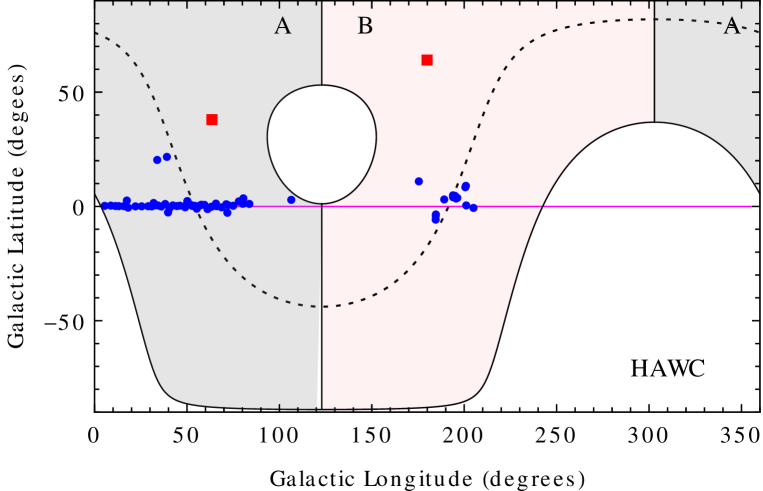
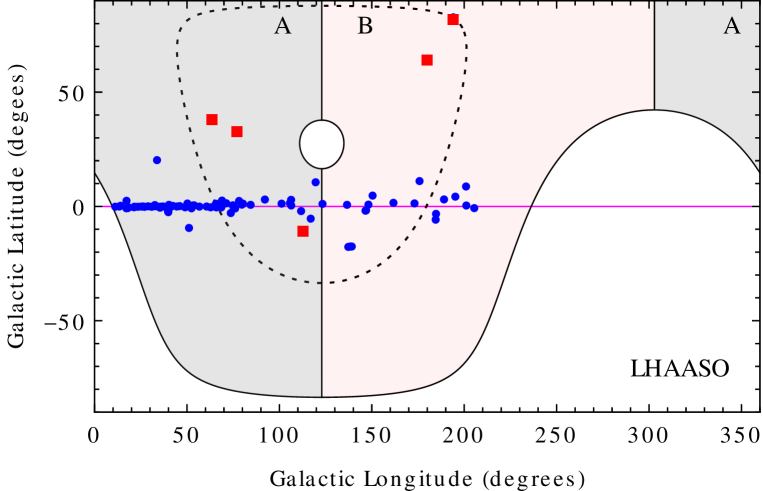
Figure 1: The two panels show the position of the gamma–ray sources in the HAWC (top) HAWC:2020hrt and LHAASO (bottom) LHAASO:2023rpg catalogs in Galactic coordinates. The red squares are sources identified as extragalactic. The shaded areas indicate the regions of the celestial sphere that are observable given the positions of the two telescopes (geographic latitude $\lambda=19.0^{\circ}$ for HAWC and $29.36^{\circ}$ for LHAASO) and assuming that the maximum angle for observing the sources is $\theta_{\rm max}=45^{\circ}$ for HAWC and 50^∘ for LHAASO. The different shadings identify the two subregions A and B [see Eq. (3)] where the sensitivity for gamma–ray observations are equal. The dashed line indicates the points of celestial declination equal to the telescope geographic latitude ($\delta=\lambda$) that corresponds to the points with trajectories that transit through the local zenith.

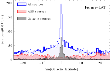
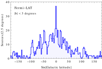
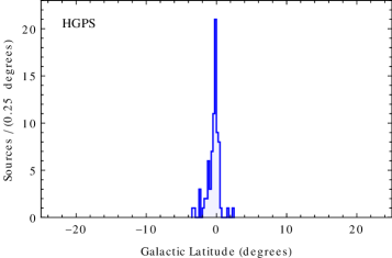
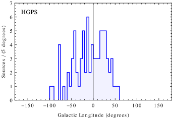
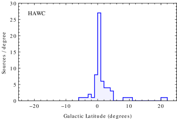
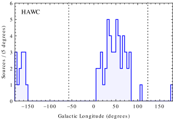
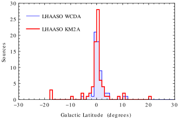
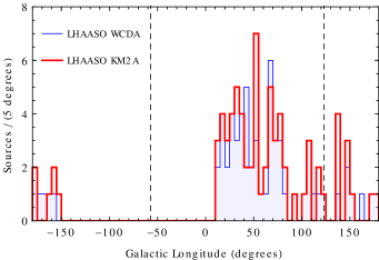
Figure 2: Distributions in Galactic latitude and longitude for sources in different gamma–ray catalogs. Top row for Fermi–LAT Fermi-LAT-4FGL-dr4 , second row for HESS–HGPS HESS:2018pbp , third row for HAWC HAWC:2020hrt , and bottom row for LHAASO (WCDA and KM2A) LHAASO:2023rpg . In the longitude plots for HAWC and LHAASO the vertical dashed lines separate the regions in longitude that have equal sensitivity.

The sky positions (in Galactic coordinates) of the sources in the two catalogs are shown in Fig. 1. It can be seen that most of the sources are located close the Galactic equator (the line of latitude $b=0$), with distributions that are strongly dependent on the Galactic longitude. The latitude and longitude distributions of the sources in the two catalogs are shown in Fig. 2, together with the distributions for the sources in the Fermi–LAT Fermi-LAT:2019yla ; Fermi-LAT-4FGL-dr4 and HESS HESS:2018pbp catalogs.

A detailed discussion of the spectral shapes of the Galactic gamma–ray sources in the catalogs listed above is presented in our companion paper lv_spectral_shapes .

The distributions over the celestial sphere of the objects listed in the gamma–ray catalogs are determined by the space and luminosity distributions of the sources, but also by the sensitivities of the telescopes and their dependence on direction. Cherenkov telescopes are pointing instruments that observe only a small portion of the sky at any given time, so the sensitivity of such a telescope depends on the history of its observations, and can generally have a complicated dependence on direction. The situation is different for an EAS telescope, because its sensitivity, which covers a limited but large portion of the sky, has a dependence on the celestial coordinates that (to a good approximation for data taking over many sidereal days) is entirely determined by its geographic latitude, and changes only gradually and smoothly with direction. Because of these characteristics of the sensitivity (discussed in more detail below), in the present work we use only the observations of the EAS telescopes HAWC and LHAASO.

II.1 Sensitivity of Extensive Air Shower telescopes

The sensitivity of an EAS gamma–ray telescope, i.e. the minimum flux required to resolve a source is to a good approximation completely determined by the celestial declination $\delta$ of the direction of observation. This is because the sky trajectory in local coordinates of a point on the celestial sphere is determined by the declination $\delta$, since points of the same declination and different right ascension follow identical trajectories that differ only by a time shift, and because the signal from a source must be compared with the fluctuations of a background dominated by the isotropic cosmic ray flux.

A telescope located at geographic latitude $\lambda$ and observing only for zenith angle $\theta<\theta_{\rm max}$ can study the region of the celestial sphere in the declination interval:

$$\delta\in[\delta_{\rm min},\delta_{\rm max}]$$ (1)

where the limits:

$$\begin{array}[]{l}\delta_{\rm min}={\rm Max}[\lambda-\theta_{\rm max},-90^{\circ}],\\[4.26773pt] \delta_{\rm max}={\rm Min}[\lambda+\theta_{\rm max},+90^{\circ}]\end{array}$$ (2)

are the declinations of points culminating at zenith angle $\theta=\theta_{\rm max}$ and only touching the cone where measurements are possible. Points with declination equal to the latitude of the telescope ($\delta=\lambda$) culminate at the zenith, and are, to a first approximation, where the sensitivity of the telescope is best. The sensitivity for any declination can be calculated by integrating over its trajectory, and taking into account how effective area, angular resolution, and background rejection depend on the zenith angle.

The fact that the sensitivity of an EAS gammma–ray telescope is independent of right ascension makes it easier to compare the observations in two different regions of the sky if these two regions are chosen to span equal intervals of declination, and therefore have equal sensitivities. In this situation, any difference between the results of the observations for the two regions (e.g. different numbers of resolved sources) must be attributed to differences in the populations of gamma–ray sources in the respective Galactic volumes.

Studies of gamma–rays in the Milky Way are best performed using the Galactic coordinates {$\ell,b\}$. The Galactic equator (line of latitude $b=0$) is inclined with respect to the celestial equator ($\delta=0$), and the two lines intersect at two points of the celestial sphere that are opposite to each other with Galactic coordinates $\{\ell,b\}=\{\ell_{1,2},0\}$ with longitudes $\ell_{1}=32.93^{\circ}$ and $\ell_{2}=-147.07^{\circ}$. The two points $\{\ell^{*}_{\pm,},0\}$ on the Galactic equator with longitudes equidistant from $\ell_{1}$ and $\ell_{2}$ (that is with longitudes $\ell^{*}_{+}=122.93$ and $\ell^{*}_{-}=-57.07^{\circ}$) are those with the minimum and maximum declination ($\delta=\pm 62.87^{\circ}$).

This suggests dividing the celestial sphere into two equal parts by selecting the Galactic longitude ranges (both extending for $180^{\circ}$):

$$\begin{array}[]{l}{\rm Region~A}:\ell\in[\ell^{*}_{-},\ell^{*}_{+}]=[-57.07^{\circ},122.93^{\circ}]\\[7.11317pt] {\rm Region~B}:\ell\in[-180^{\circ},\ell^{*}_{-}]\oplus[\ell^{*}_{+},180^{\circ}]=[-180^{\circ},-57.07^{\circ}]\oplus[122.93^{\circ},180^{\circ}]\end{array}$$ (3)

with the property that the sensitivity of any EAS telescope is the same in both regions. This follows from the fact that points on the celestial sphere with longitudes symmetric with respect to $\ell^{*}_{\pm}$, i.e. points with Galactic coordinates $\{\ell^{*}_{\pm}+\Delta\ell,b\}$ and $\{\ell^{*}_{\pm}-\Delta\ell,b\}$ have identical declination. Note that region A contains the Galactic Center, and region B the anticenter.

The two sky regions A and B can also be defined in terms of celestial coordinates as the right ascension ranges:

$$\begin{array}[]{l}{\rm Region~A}:\alpha\in[\alpha_{1},\alpha_{2}]=[-167.14^{\circ},+12.86^{\circ}]\\[7.11317pt] {\rm Region~B}:\alpha\in[-180^{\circ},\alpha_{1}]\oplus[\alpha_{2},180^{\circ}]=[-180^{\circ},-167.14^{\circ}]\oplus[12.86^{\circ},180^{\circ}]\end{array}$$ (4)

where the right ascensions $\alpha_{1}=-167.14^{\circ}$ and $\alpha_{2}=\alpha_{2}+180^{\circ}$ are the right ascensions of the two points on a line in the sky of constant declination $\delta$ that have the minimum and maximum Galactic latitude. In this second definition it is manifest that the sensitivity of a telescope is equal in both sky regions.

An EAS telescope, can observe only a limited portion of the celestial sphere [see Eq.(2)] and this visible region of the sky can be divided into two parts of equal solid angle and sensitivity, one belonging to region A and the other to region B. The visible part of the celestial sphere for the HAWC and LHAASO telescopes, and their subdivisions into region A and region B are shown in Fig. 1 assuming gamma–ray observations for a maximum zenith angle of 45^∘ for HAWC and 50^∘ for LHAASO.

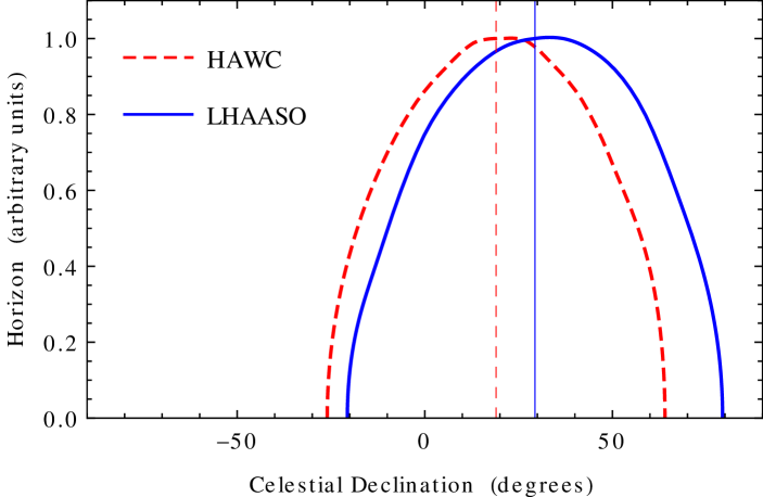
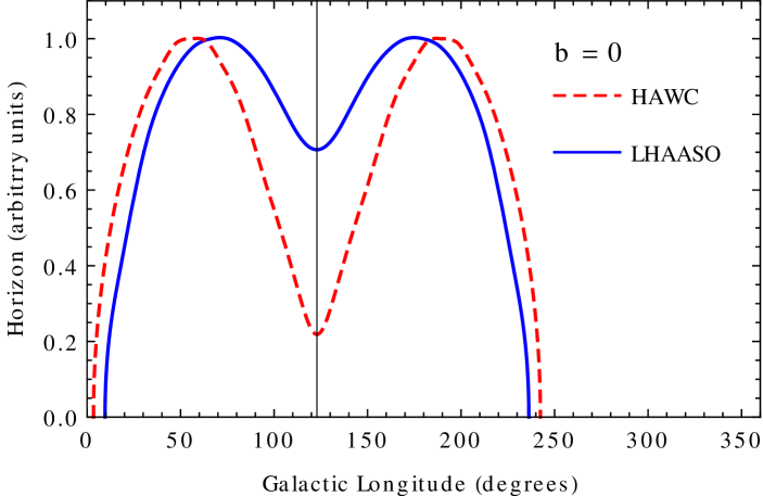
Figure 3: The top panel shows the declination dependence of the horizon to resolve point–like gamma–ray sources for the HAWC and LHAASO–KM2A telescopes plotted as a function of celestial declination. The absolute value of the horizon scales with the source luminosity ($D_{H}\propto L^{1/2}$). The horizon for LHAASO–WCDA has a very similar declination dependence. The vertical lines correspond to a declination equal to the geographic latitude of the telescope, where (to a good approximation) the sensitivity is best, and the horizon is largest. The bottom panel shows again the horizon for points on the Galactic equator ($b=0$) plotted as a function of the longitude for the two telescopes.

In HAWC:2020hrt and LHAASO:2023rpg the HAWC and LHAASO collaborations give plots of the minimum flux required to resolve a point–like source as a function of declination. The declination dependencies of the telescope sensitivities are shown in Fig. 3 re–expressed in terms of the relative size of the horizon, that is the maximum distance to resolve a point–like source. The sensitivity of a telescope is best and the horizon is largest (to a good approximation) for $\delta\approx\lambda$ when the source transits through the local zenith, and the horizon vanishes for declinations $\delta_{\rm min}$ and $\delta_{\rm max}$ when a source only grazes the observation cone $\theta<\theta_{\rm max}$.

Since most of the Galactic sources are observed near the Galactic equator it can be useful to show the sensitivity as a function of Galactic longitude along the equator ($b=0$). For the LHAASO detector, located at longitude $\lambda\simeq 29.36^{\circ}$, and assuming an observation cone with $\theta_{\rm max}=50^{\circ}$, the equator is visible only for longitudes in the range $\ell\in[9.6^{\circ},236.3^{\circ}]$. For the HAWC telescope, located at geographic latitude $\lambda=19.0^{\circ}$, and assuming an observation cone with $\theta_{\rm max}=45^{\circ}$, the Galactic equator is visible in the longitude interval $\ell\in[3.4^{\circ},242.4^{\circ}]$. For both telescopes, for the reasons outlined above, the dependence of the sensitivity on the longitude is symmetrical around the longitude $\ell=\ell^{*}_{+}=122.93^{\circ}$, with the part of the sky with $\ell<\ell^{*}_{+}$ in region A , and the part of the sky with $\ell>\ell^{*}_{+}$ in region B.

II.2 Resolved and unresolved gamma–ray sources

A gamma–ray source is completely described by its position, luminosity, spectral shape and morphology. A precise description of the spectral shape and morphology of a source can be quite complicated, and in the following we will make some simplifications. For the spectral shape, we will assume that, in a not too large energy interval, it can be reasonably well approximated by a simple power–law form of slope $\alpha_{j}$ ($\phi_{j}(E)\propto E^{-\alpha_{j}}$) [for a discussion of the spectral shapes of the Galactic gamma ray sources see lv_spectral_shapes ].

The integrated flux in the interval $[E_{\rm min},E_{\rm max}]$ can then be expressed (neglecting absorption) in the form:

$$\Phi_{j}=\frac{L_{j}}{4\,\pi\,\langle E_{j}\rangle\;D_{j}^{2}}~,$$ (5)

where $D_{j}=|\vec{x}_{j}-\vec{x}_{\odot}|$ is the distance of the source from the solar system (located at $\vec{x}_{\odot}$), and $L_{j}$ is the source luminosity in the same energy interval (left implicit in the notation). The quantity $\langle E_{j}\rangle$ is the average energy of the photons in the interval of interest:

$$\langle E_{j}\rangle=E_{\rm min}~\left(\frac{\alpha_{j}-1}{\alpha_{j}-2}\right)\;\left[1-\left(\frac{E_{\rm min}}{E_{\rm max}}\right)^{\alpha_{j}-2}\right]~.$$ (6)

The morphology of a source will be described with the single parameter $R$ that gives its linear size.

A gamma–ray source is resolved in the observations of a telescope if its integrated flux is larger than a minumum value $\Phi_{\rm min}$ which in general depends on the direction of observation $\Omega$, the angular size of the source $\delta\theta_{s}$ and its spectral shape. In the following we assume that the sources, in the considered energy interval, have approximately the same spectral index, and parameterize the dependence of the minimum flux on the source size with the form:

$$\Phi_{\rm min}(\Omega,\delta\theta_{s})\simeq\Phi_{\rm min}^{0}(\Omega)~~\sqrt{1+\left(\frac{\delta\theta_{s}}{\delta\theta_{\rm exp}}\right)^{2}}~.$$ (7)

In this expression $\Phi_{\rm min}^{0}(\Omega)$ is the minimum flux to resolve a point–like source in the direction $\Omega$, and $\delta\theta_{\rm exp}$ is the angular resolution of the telescope. The dependence of the minimum flux on the source angular size can be derived from the assumption that the minimum observable signal from a source is proportional to the size of the fluctuations of an isotropic background (dominated by the hadronic cosmic ray flux) integrated over a solid angle region of dimension $\delta\Omega\propto(\delta\theta_{s}^{2}+\delta\theta_{\rm exp}^{2})$.

The condition $\Phi_{j}>\Phi_{\rm min}$ can be a expressed as an upper limit on its distance $D_{j}\leq D_{H}$, where the horizon $D_{H}$ is a function of the source luminosity and linear size. For a point–like object, the horizon (leaving the dependence on the direction $\Omega$ implicit) takes the simple form:

$$D_{\rm H}^{0}(L)=\sqrt{\frac{L}{4\pi\,\langle E\rangle\;\Phi_{\rm min}^{0}}}$$ (8)

that grows with the source luminosity $\propto\sqrt{L}$. If the source has a linear size $R$ the horizon distance is smaller and takes the more general form:

$$D_{\rm H}(L,R)=D_{H}^{0}(L)~\sqrt{\sqrt{1+\frac{1}{4\,x^{4}}}-\frac{1}{2\,x^{2}}}\simeq\begin{cases}D_{H}^{0}(L)~x\propto L&{\rm for}~~x\ll 1\\[7.11317pt] D_{H}^{0}(L)\propto\sqrt{L}&{\rm for}~~x\gg 1\end{cases}$$ (9)

where the adimensional quantity $x$:

$$x=\frac{D_{H}^{0}(L)}{R/\delta\theta_{\rm exp}}$$ (10)

is the ratio between the horizon for a point–like source of luminosity $L$ and the distance $R/\delta\theta_{\rm exp}$ where a source of size $R$ has an angular extension equal to the detector resolution. Note that if the horizon distance is much smaller than $R/\delta\theta_{\rm exp}$, its dependence on the luminosity is $\propto L$.

II.3 Resolved sources in the HAWC and LHAASO catalogs

The number of Galactic sources in the HAWC and LHAASO catalogs observed in regions A and B (which are similar but not not identical for the two telescopes) are listed in Table 1.

Table 1: Numbers of high energy Galactic gamma–ray sources in different sky regions for the HAWC and LHAASO catalogs. For the LHAASO catalog the three lines show the sources detected by the WCDA array, the KM2A array and the subset of the KM2A sources detected also above 100 TeV. Region A corresponds to the Galactic longitude range: $\ell\leq\ell^{*}$ and region B to the complementary range $\ell>\ell^{*}$, with $\ell^{*}=122.9^{\circ}$.

	All longitudes				$|b|\leq 3^{\circ}$				$|b|>3^{\circ}$
Telescope	$N$	$N_{A}$	$N_{B}$	$N_{A}/N_{B}$	$N$	$N_{A}$	$N_{B}$	$N_{A}/N_{B}$	$N$	$N_{A}$	$N_{B}$	$N_{A}/N_{B}$
HAWC	63	49	14	$3.5\pm 1.1$	48	46	2	$23.\pm 17.$	15	3	12	$0.25\pm 0.16$
LHAASO	86	66	20	$3.3\pm 0.84$	70	61	9	$6.8\pm 2.4$	16	5	11	$0.45\pm 0.25$
LHAASO–WCDA	65	51	14	$3.6\pm 1.1$	55	49	6	$8.2\pm 3.5$	10	2	8	$0.25\pm 0.2$
LHAASO–KM2A	75	58	17	$3.4\pm 0.94$	62	54	8	$6.8\pm 2.6$	13	4	9	$0.44\pm 0.27$
LHAASO–KM2A-High	44	36	8	$4.5\pm 1.8$	34	32	2	$16.\pm 12.$	10	4	6	$0.67\pm 0.43$

In the case of LHAASO we show the results for the measurements made by the WCDA and KM2A arrays, and also the results for the KM2A sources that have measurable fluxes for energies $E\geq 100$ TeV. When looking at these numbers one should keep in mind that the sensitivity of the telescopes in the A and B regions is identical. The number of sources $\{N_{A},N_{B}\}$ for the four cases are: {49,14}, {51,14}, {68,17} and {36,8} (for HAWC, LHAASO–WCDA, LHAASO–KM2A and LHAASO–high respectively) with $N_{A}/N_{B}$ ratios between 3.5 and 4.5. The numbers of resolved sources are small, but it is clear that there is a large asymmetry, with more sources in the sky region closer to the Galactic Center. This suggests that the sources can be resolved at distances larger than a few kiloparsecs. Such a conclusion is clearly important for estimating the flux from the ensemble of unresolved sources, located beyond this horizon. In the following we will try to obtain a more precise estimates for the horizon and the unresolved flux.

Table 1 also lists the number of sources in two different ranges of latitude ($|b|\leq 3^{\circ}$ and $|b|>3^{\circ}$). Most of the sources are observed at small $|b|$, and the ratio $N(|b|\leq 3^{\circ})/N({\rm all}~b)$ is 0.76 for HAWC and 0.81 for LHAASO. This indicates that the sources are distributed in a thin disk, and that the horizon is much larger than the thickness of this disk.

Table 1 also gives the number of resolved sources of small ($|b|\leq 3^{\circ}$) and large ($|b|>3^{\circ}$) latitude in the A and B sky regions. These numbers reveal the surprising fact that for sources at large latitude one observes more sources in region B, toward the Galactic anti–center. The number of sources $\{N_{A}(|b|<3^{\circ}),N_{B}(|b|<3^{\circ})\}$ in the same four catalogs as before are: {3,12}, {2,8}, {4,9} and {4,6}, and the ratio $N_{A}/N_{B}$ is significantly less than unity. This result, that is also clearly visible in Fig.1 where it can be seen that the latitude spread for sources at large $|\ell|$ is larger than for sources closer to the Galactic Center. This result is due to the fact that the sources observed at large $|b|$ are near the Solar system, and their space distribution is determined by the position and shape of the spiral arms of the Galaxy.

This result suggests that smooth, cylindrically symmetric models of the space distributions of the sources are not adequate to describe these features, and that a precise and detailed modeling of the spiral arms is required. For this reason (and because of the small statistics available at the moment) we postpone the study of the declination dependence of the gamma–ray sources to a future work, and in the following we will base our discussion on the comparison of only two large sky regions, because in this case the sensitivity to the precise modeling of the the space distributions of the sources is much reduced.

III Diffuse Galactic gamma–ray flux measurements

In the the energy range 0.1–100 GeV the flux generated by the emission from cosmic rays propagating in the interstellar medium has been well measured over the entire celestial sphere by the Fermi–LAT telescope Fermi-LAT:2012edv ; Fermi-LAT:2016zaq . Below few GeV the emission generated by relativistic electrons and positrons (via Compton scattering and bremsstrahlung) is important. At higher energies most of the diffuse flux is generated by the hadronic mechanism, where gamma–rays are created in the decay of mesons (mostly $\pi^{\circ}$) produced in the inelastic collisions of protons and nuclei with interstellar gas. The hadronic mechanism is also expected to be dominant in the TeV and PeV energy range.

The Fermi–LAT observations of the diffuse flux encode information that is very important for high energy astrophysics. The crucial problem is to determine whether or not cosmic rays in different parts of the Milky Way have spectra of the same shape as measured in the vicinity of the Earth. There is currently some controversy about the interpretation of the Fermi–LAT measurements (see for example Gaggero:2014xla ; Yang:2016jda ), and observations at higher energies are of crucial importance to shed light on the problem.

Measurements of the diffuse gamma–ray flux for $E\gtrsim 1$ TeV are possible only with telescopes at ground level, and therefore measurements have been obtained only in some limited regions of the sky.

• The ARGO–YBJ telescope ARGO-YBJ:2015cpa has published a measurement of the diffuse flux in the (approximate) energy range [0.35,2] TeV for the sky region of Galactic latitude $|b|<5^{\circ}$ and longitude $25^{\circ}<\ell<100^{\circ}$.

• The Tibet–AS$\gamma$ telescope TibetASgamma:2021tpz has published measurements of the diffuse flux in the (approximate) energy range [10²,10³] TeV in two sky regions (in partial overlap) {$|b|<5^{\circ}$, $25^{\circ}\leq\ell\leq 100^{\circ}$} and {$|b|<5^{\circ}$, $50^{\circ}\leq\ell\leq 200^{\circ}$}. (note that the first region in the same as that used by ARGO–YBJ).

• The LHAASO–KM2A detector LHAASO:2023gne has published measurements of the diffuse gamma–ray flux in the two regions of the sky around the Galactic plane: {$|b|<5^{\circ}$, $15^{\circ}\leq\ell\leq 125^{\circ}$} and {$|b|<5^{\circ}$, $125^{\circ}\leq\ell\leq 235^{\circ}$}. These two regions have the same solid angle extent, with the second (Outer–Galaxy) centered on the Galactic anticenter and the other (Inner–Galaxy) approaching but not reaching the Galactic center.

• The HAWC telescope HAWC:2023wdq has also published a measurement of the diffuse gamma–ray flux in the smaller sky region {$|b|<4^{\circ}$, $43^{\circ}\leq\ell\leq 73^{\circ}$} The HAWC publication also includes flux estimates in smaller portions of this region.

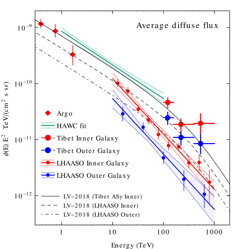
Figure 4: Measurements of the average diffuse gammma–ray flux at high energy obtained by different telescopes: ARGO-YBJ ARGO-YBJ:2015cpa , Tibet AS$\gamma$ TibetASgamma:2021tpz , HAWC HAWC:2023wdq and LHAASO LHAASO:2023gne in different sky regions. The predictions of the average diffuse flux for the factorized model in LV-2018 Lipari:2018gzn for the same sky regions are also shown in the figure.

The diffuse flux measurements of ARGO, Tibet–As$\gamma$, LHAASO and HAWC are shown in Fig. 4 in the form of the average flux in the sky region of observation. It should be noted that the measurements are made in different regions of the sky and therefore a comparison of the results requires a careful discussion of the angular dependence of the flux.

In Fig. 4 we also show (as thin lines) the predictions of the diffuse flux of the factorized model of reference Lipari:2018gzn (hereafter LV–2018 ). This model assumes that the angular distribution of the diffuse flux is energy independent and remains equal to what has been observed by Fermi–LAT for energy $E\simeq 10$ GeV, and the energy dependence of the flux obtained assuming that for $E\gtrsim 10$ GeV the emission is dominated by the hadronic mechanism (see below) and can therefore be calculated, and that the shape of the cosmic ray spectra in all points of the Galacy is identical to what is observed in the vicinity of the Earth. Uncertainties in the shape of the energy spectrum are then controlled by the modeling of the observed cosmic ray spectra and composition in the range where only indirect EAS measurements are possible. The resulting gamma–ray spectrum is then in first approximation a power law with a spectral index $\alpha\approx 2.7$, which gradually softens for $E\gtrsim 10^{2}$ TeV, due to the “Knee” in the primary particle spectrum.

Table 2 shows the relative magnitude of the average diffuse flux observed by Fermi–LAT in different sky regions at $E\simeq 12$ GeV, when the most of the flux is produced by the hadronic mechanism.

Table 2: Relative magnitude of the average diffuse (interstellar emission) gamma–ray flux estimated from the Fermi–LAT observations at $E=12$ GeV in the sky regions where measurements at high energies by Tibet–AS$\gamma$ TibetASgamma:2021tpz , LHAASO LHAASO:2023gne and HAWC HAWC:2023wdq are available. For the two LHAASO regions the average flux is also calculated in the solid angle remaining after the masking of known sources.

Sky region	Latitude	Longitude	$\langle\phi\rangle_{\rm no-mask}$	$\Delta\Omega_{\rm mask}/\Delta\Omega$	$\langle\phi_{\rm mask}\rangle/\langle\phi_{\rm no~mask}\rangle$	$\langle\phi\rangle_{\rm mask}$
LHAASO: Inner Galaxy	$|b|<5^{\circ}$	$15^{\circ}\leq\ell\leq 125^{\circ}$	1	0.617	0.622	1
LHAASO: Outer Galaxy	$|b|<5^{\circ}$	$125^{\circ}\leq\ell\leq 235^{\circ}$	0.337	0.802	0.984	0.534
HAWC: Innner Galaxy	$|b|<4^{\circ}$	$43^{\circ}\leq\ell\leq 73^{\circ}$	0.960	–	–	1.54
Tibet–AS$\gamma$: Inner Galaxy	$|b|<5^{\circ}$	$25^{\circ}\leq\ell\leq 100^{\circ}$	1.027	–	–	1.65
Tibet–AS$\gamma$: Outer Galaxy	$|b|<5^{\circ}$	$50^{\circ}\leq\ell\leq 200^{\circ}$	0.530	–	–	0.852

From the table one can see that in three regions (Tibet–AS$\gamma$ Inner Galaxy, LHAASO Inner–Galaxy, and HAWC) the average fluxes are approximately equal with ratios (1:0.97:0.93), while the Tibet–AS$\gamma$ Outer–Galaxy region has a flux that is a factor 0.53 smaller, and the LHAASO Outer–Galaxy region a fraction 0.33 smaller. It is important to note, however, that the LHAASO diffuse flux measurements are made after masking the points in the sky around resolved gamma–ray sources, and therefore exclude 38.3% and 19.8% of the Inner–Galaxy and Outer–Galaxy regions, respectively. The gamma–ray sources are mostly located at small Galactic latitudes, and therefore the masking mostly excludes points at small $|b|$, where also the flux due to the interstellar emission is higher. Using the results of Fermi–LAT to model the angular distribution of the diffuse flux, one can estimate that the average fluxes in the solid angle reduced by the masking are lower by factors of 0.622 and 0.984 for the Inner and Outer–Galaxy regions, respectively.

One should keep in mind that what is observed as a diffuse gamma–ray flux can be considered, at least in first approximation, as formed by the sum of a (truly diffusive) component generated by the interstellar space emission, and the flux due to the ensemble of all unresolved sources:

$$\Phi_{\rm diffuse}^{\rm data}=\Phi_{\rm ism}+\Phi^{\rm unresolved}_{\rm sources}~.$$ (11)

In this expression the fluxes are integrated in energy over the interval $[E_{\rm min},E_{\rm max}]$ and in angle over the sky region $\Delta\Omega$, that are both left implicit. Disentangling these components is of great importance.

A comparison of the diffuse flux observations by LHAASO and Tibet–AS$\gamma$ will be briefly discussed below in section VI.1.

IV The Horizon method

The main goal of the present work is to estimate luminosity of the ensemble of gamma–ray sources in the Galaxy, and the flux of unresolved sources extrapolating from the information obtained from the observations of the resolved sources. To perform this task we will use a simple method based on the study of the distribution in celestial coordinates of the sources contained in the catalogs of the EAS telescopes.

To illustrate the idea behind this method one can consider a simple, ideal situation where the Milky Way contains $N_{\rm tot}$ identical point–like sources of luminosity $L_{0}$, and a telescope observes a region $\Delta\Omega$ of the celestial sphere, with a sensitivity independent of the direction, and therefore resolving all sources within the horizon distance $D_{H}$, that is a function of the source luminosity according to Eq.(8).

We will now assume that the space distribution of the gamma–ray sources is known. Of course, this space distribution should be determined using present and future observations, however, it is reasonably safe to assume that the gamma–ray sources have a distribution similar to other components of the Milky Way (such as stars, pulsars or supernova remnants) and form a thin disk that extends for several kiloparsecs around the Galactic center, with the Solar system placed at a radius of approximately 8.5 kpc.

The result that the telescope has resolved $N_{s}$ sources does not allow to infer the values of $L_{0}$ and $N_{\rm tot}$ because the observations can be reproduced by an infinite number of solutions. In some solutions the Galaxy contains many faint sources, with the telescope resolving only close objects, in other solutions the Galaxy contains a smaller number of brighter objects that can be resolved in a larger volume.

To resolve this ambiguity one can divide the sky into two parts: region A toward the Galactic Center and region B toward the anti-center, that contain $N_{A}$ and $N_{B}$ resolved sources. It is not strictly necessary, but it is convenient to choose the two regions as having equal solid angle ($\Delta\Omega_{A}=\Delta\Omega_{B}$). It is now easy to see that the pair of values $\{N_{A},N_{B}\}$ can be mapped into the pair of quantities $\{L_{0},N_{\rm tot}\}$ (and viceversa).

In fact the ratio $N_{A}/N_{B}$ depends only on the size of the horizon $D_{H}$ and therefore only on $L_{0}$ (the luminosity of the individual sources). Since the source density increases toward the Galactic center, a ratio $N_{A}/N_{B}$ of the order of unity indicates that all resolved sources are near the Solar system, and therefore that the horizon $D_{H}$ is short and the luminosity $L_{0}$ is small. Increasing the horizon $D_{H}$ (and therefore the luminosity $L_{0}$) the ratio $N_{A}/N_{B}$ grows because the volume subtended by the solid angle $\Delta\Omega_{A}$ (toward the Galactic Center) and of radius $D_{H}$ contains a larger fraction of the Milky Way than the corresponding volume subtended by the solid angle $\Delta\Omega_{B}$ (toward the anti–center). The ratio $N_{A}/N_{B}$ reaches a maximum asymptotic value for very large $L_{0}$, when the horizon $D_{H}$ becomes larger than the maximum extension of the Galaxy along any direction (that is for $D_{H}\gtrsim 50$ kpc) and all Galactic gamma–ray sources in the field of view of the telescope are resolved.

Having estimated $L_{0}$ from the ratio $N_{A}/N_{B}$, it then straightforward to infer the total number of sources and the total luminosity of the Milky Way from the number of resolved sources $(N_{A}+N_{B})$. It is also obvious that having determined the horizon beyond which the sources are not resolved, one can make use of the (assumed) space distribution of the sources, to compute the flux of unresolved sources in any desired direction.

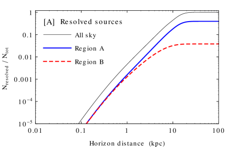
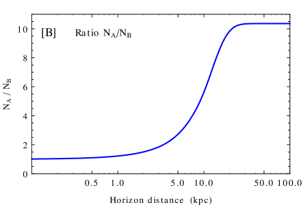
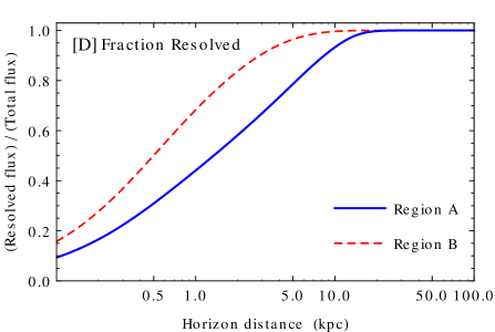
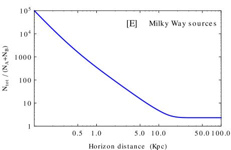
Figure 5: This figure illustrates how the “horizon method” allows to estimate: the luminosity $L_{0}$ of the individual gamma–ray sources, the total luminosity $L_{\rm tot}$ of all Milky Way sources, and the flux of unresolved sources on different sky regions. In this example we assume that the Galactic sources are all point–like and identical, and that the minimum flux $\Phi_{\rm min}$ to resolve a source is direction independent. The calculation is performed for the LHAASO telescope, using the cylindrically symmetric model for the space distribution of the sources. The six panels show different quantities plotted as a function of the horizon distance that is in one–to–one correspondence with the luminosity $L_{0}$ [see Eq.(8)]. Panel [A] shows the number of resolved sources for all the sky, and for regions A and B. Panel [B] shows the ratio $N_{A}/N_{B}$ of the numbers of resolved sources in the two regions. Panel [C] shows the flux of resolved sources in all sky and in regions A and B divided by the quantity $L_{\rm tot}/(4\pi\,\langle E\rangle)$ (with $\langle E\rangle$ the average energy of photons on the interval considered). Panel [D] shows the fraction of the source flux due to resolved sources in region A and region B. Panel [E] shows the ratio $N_{\rm tot}/(N_{A}+N_{B})$ between the total number of sources in the Milky Way and the number of resolved sources. Panel [F] shows the ratio of the total luminosity of the Milky Way and the quantity ($4\pi\,\langle E\rangle\,\Phi_{\rm min}\,(N_{A}+N_{B})$).

The different steps of the horizon method are shown graphically in the six panels of Fig. 5 where different quantities associated with the properties of the Galactic gamma–ray sources are plotted as a function of the horizon distance. This example is calculated assuming the cylindrically symmetric model for the space distribution of the gamma–ray sources discussed in the appendix A.1, the simple model of point–like identical sources and a direction independent minimum flux $\Phi_{\rm min}$ (in the sky region visible by the LHAASO telescope). It is simple to see how the measurement of $N_{A}$ and $N_{B}$ allows to determine $L_{0}$, $L_{\rm tot}$ and the resolved and unresolved fluxes in the two sky regions A and B. Note in panel F how the estimate of the total Galactic luminosity is approximately constant for the horizon in the interval 1–10 TeV.

IV.1 Modeling of the Galactic sources

In the following we will apply the simple geometrical idea introduced above to interpret the observations of the HAWC and LHAASO telescopes. As already discussed, the optimal way to divide the portion of the celestial sphere observed by an EAS telescopes into two parts is to use the subdivision descrived by Eq.(3) or equivalently Eq.(4). The two regions obtained in this way are of equal solid angle, and have (in very good approximation) identical sensitivities, therefore any difference in the number of observed sources must be attributed to real differences in the distributions of the gamma–ray sources.

We want to perform a reasonably realistic calculation, however we will have to introduce some simplifications:

1. We will assume that all sources have the same spectral shape: a power–law of slope $\alpha$. Our discussion will always refer to the flux and luminosity in rather narrow energy intervals, so that this will be a reasonable approximation.

2. We will also assume that all sources have the same linear size $R$, and then study how the results depend on the value of $R$.

3. We will assume the factorization of the space and luminosity dependence of the source distributions:

   $$\frac{dN_{s}}{d^{3}x\,dL}=f(\vec{x})\,\frac{dN_{s}}{dL}$$ (12)

   This factorization hypothesis is motivated by the search for simplicity, and should be critically reviewed in future studies.

In Eq.(12) the function $f(\vec{x})$ describes the space distribution of the sources and, without any loss of generality, is normalized to unity:

$$\int d^{3}x~f(\vec{x})=1~.$$ (13)

In the following we will use a model with cylindrical symmetry, based on previous works of Yusifov and Kucuk Yusifov:2004fr that fit the distribution of pulsars in the Galaxy, and a model that includes the spiral structure of the Milky Way based on the studies of Reid et al. Reid:2019 that fit the space distribution of high–mass star forming regions. Both models are presented in the appendix A.

For the luminosity distribution of the sources we will consider the simple toy model where all sources are identical with luminosity $L_{0}$:

$$\frac{dN_{s}}{dL}=\frac{L_{\rm tot}}{L_{0}}~\delta[L-L_{0}]$$ (14)

and a more realistic model, a power law with exponential cutoff:

$$\frac{dN_{s}}{dL}=\frac{L_{\rm tot}}{\Gamma(2-\gamma)\;L_{*}^{2}}~\left(\frac{L}{L_{*}}\right)^{-\gamma}~\exp\left[-\frac{L}{L_{*}}\right]~.$$ (15)

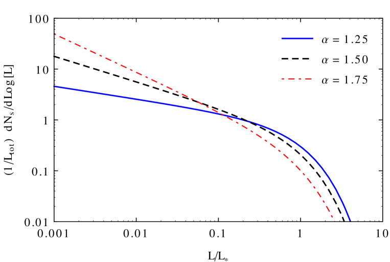
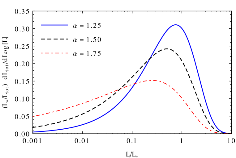
Figure 6: The top panel shows the luminosity distribution with the form of Eq. (15) (a power–law with exponential cutoff), plotted in the form $L\,dN_{s}/dL=dN_{s}/d\log L$ for three values of the exponent: $\gamma=1.25,1.5$ and 1.75. In the absence of a low luminosity cutoff the total number of sources diverge. The bottom panel shows again the luminosity distribution (for the same three values of the exponent) in the form $L^{2}\,dN_{s}/dL=dL_{\rm tot}/d\log L$ plotted with a linear $y$ scale. The total luminosity remains finite.

This distribution is determined by the three parameters {$L_{\rm tot}$, $L_{*}$, $\gamma\}$, with $L_{\rm tot}$ the total luminosity of the ensemble of all Galactic sources, $L_{*}$ a characteristic luminosity, and the exponent $\gamma$ controls the importance of faint sources. A luminosity distribution of very similar form (a power-law between sharp limits $L_{\rm min}$ and $L_{\rm max}$) was introduced by Strong in Strong:2006hf , and has subsequently been used by other authors Steppa:2020qwe ; Cataldo:2020qla . The form of Eq.(15) does not have a low luminosity cutoff, and replaces the sharp high energy cutoff with a more realistic exponential one. The lack of the low energy cutoff implies that the total number of sources in the Galaxy diverges for $\gamma\geq 1$, while the total luminosity diverges for $\gamma\geq 2$. An illustration of luminosity distribution in Eq.(15) is given in Fig. 6, where one can see that, for an exponent $\gamma$ smaller and not to close to two, the total luminosity of the Galactic sources, and therefore the total source flux, is mostly due to objects that have a luminosity around $L_{*}$.

It could appear surprising that the absolute normalization of the luminosity distribution is parametrized with $L_{\rm tot}$, the total power of the Milky Way gamma–rays sources, and not with $N_{\rm tot}$, the total number of sources. This is however a better choice, because the total number of sources in the Galaxy is a quantity that can be ambiguous and misleading, and is in fact essentially impossible to measure, because the Galaxy very likely contains a large number of very faint sources that give a negligible contribution to both the total flux and the total luminosity. In fact, as already discussed, the total number of sources in the Galaxy diverges for an exponent $\gamma\geq 1$, but this divergence is harmless, as long as the total luminosity of the Galaxy remains finite.

The number of sources resolved by a telescope in the sky region $\Delta\Omega$ can be calculated integrating over the luminosity and space distributions of the source:

$$N_{s}(\Delta\Omega)=\int dL~\frac{dN_{s}}{dL}~\int_{\Delta\Omega}d\Omega~\int_{0}^{D_{H}(L,\Omega)}dt~t^{2}~f[\vec{x}_{\odot}+\hat{n}(\Omega)\,t]$$ (16)

where the integration in space is extended up to the horizon $D_{H}(L,\Omega)$ that depends on the luminosity of the source and on the sensitivity of the telescope in that direction [see Eq.(9)].

The total flux from all (resolved and unresolved) gamma–ray sources in the sky region $\Delta\Omega$ can be calculated as:

$$\Phi_{\rm sources}^{\rm all}(\Delta\Omega)=\frac{L_{\rm tot}}{4\,\pi\;\langle E\rangle}~\int_{\Delta\Omega}d\Omega~\int_{0}^{\infty}dt~f[\vec{x}_{\odot}+\hat{n}(\Omega)\,t]$$ (17)

and is proportional to the total Galactic luminosity and is independent of the form of the luminosity distribution. The flux from unresolved sources in the same sky region does depend on the luminosity distribution and can be obtained with an integration similar to the one in Eq.(16):

$$\Phi_{\rm sources}^{\rm unresolved}(\Delta\Omega)=\frac{1}{4\,\pi\;\langle E\rangle}~\int dL~L~\frac{dN_{s}}{dL}~\int_{\Delta\Omega}d\Omega~\int_{D_{H}(L,\Omega)}^{\infty}dt~f[\vec{x}_{\odot}+\hat{n}(\Omega)\,t]$$ (18)

where the space integration extends from the horizon to infinity.

For a luminosity distribution of the form of Eq. (15), the sky distribution of the resolved sources can be used to estimate the parameters $L_{*}$ and $L_{\rm tot}$. Assuming the validity of the factorization hypothesis, a form for the space distributions of the sources, and a value for the exponent $\gamma$, then it is straightforward to map the pair $\{N_{A},N_{B}\}$ (the numbers of resolved sources in region A and B) into the parameters $\{L_{*},L_{\rm tot}\}$ following the same method outlined above for the case of identical sources. The ratio $N_{A}/N_{B}$ is a function only of $L_{*}$, and then the absolute number of resolved sources allows to estimate $L_{\rm tot}$.

It should be noted that for the power–law luminosity model, if the exponent is $\gamma\geq 1$ (and the total number of sources in the Galaxy diverges), in the limit $L_{*}\to\infty$, the number of resolved also diverges, as more and more faint sources can be identified. The rate of the divergence of the number of resolved sources depends on the exponent $\gamma$ and it is faster for larger exponents with the form: $N_{\rm resolved}\propto L_{*}^{(\gamma-1)}$.

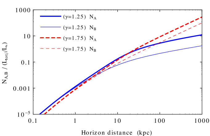
Figure 7: Number of resolved sources in region A and B of the LHAASO detector calculated assuming the cylindrically symmetric space distribution described in appendix A.1 and the power–law with exponential cutoff for the luminosity distribution [see Eq.(15)]. The number of sources is plotted as a function of the horizon for the critical luminosity $L_{*}$ in a direction of declination $\delta=\lambda$. The curves are calculated for two values of the exponent of the power law: $\gamma=1.25$ and $\gamma=1.75$. For large values of $L_{*}$, when the horizon is larger than the linear extension of the Galaxy, the number of resolved sources increase as a power law $N_{A,B}\propto L_{*}^{\gamma-1}\propto D_{H}^{2(\gamma-1)}$. Note also how the ratio $N_{A}/N_{B}$ for a large horizons is smaller for the larger exponent $\gamma$.

The divergence can be also expressed in terms of the horizon $D_{*}=D_{H}(L_{*},\Omega)$ for a source of luminosity $L_{*}$ in an fixed (arbitrary) direction: $N_{\rm resolved}\propto D_{*}^{2(\gamma-1)}$. This is illustrated in Fig. 7 that plots, for the LHAASO detector, the number of resolved sources in regions A and B as a function of the horizon $D_{*}=D_{H}(L_{*},\delta=\lambda)$ for the critical luminosity $L_{*}$ in a direction of declination $\delta=\lambda$ for two values of the exponent $\gamma$. For large $L_{*}$ the numbers of resolved sources in different angular regions grow at the same rate, and therefore the ratio $N_{A}/N_{B}$ becomes asymptotically a constant, that depends on the exponent $\gamma$.

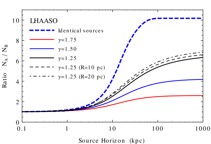
Figure 8: The top panel shows how the ratio $N_{A}/N_{B}$ of gamma–ray sources observable in region A and region B for the LHAASO telescope depends on the horizon for source resolution, in the case of identical sources and for the luminosity distribution of Eq. (15) (a power–law with exponential cutoff). The horizon indicated in the $x$–axis is for a source with celestial declination $\delta=\lambda$ (with $\lambda$ the geographic latitude of the telescope). For other directions the horizon is shorter, and depends on $\delta$ with the form shown in Fig. 3. One line is for point–like identical sources, the other lines are for a power–law luminosity distribution, and in this case the horizon indicated in the $x$–axis is for sources with the cutoff luminosity $L_{*}$, and scales with $L$ according to Eq. (9). Three curves are for point–like sources with three values of the exponent: $\gamma=1.25$, 1.50 and 1.75. For $\gamma=1.25$ also the cases with sources of linear size $R=10$ pc and 20 pc are shown.

This is shown in Fig. 8 that plots the ratio $N_{A}/N_{B}$ as a function of the horizon $D_{0}=D_{H}(L_{0},\delta=\lambda)$ or $D_{*}=D_{H}(L_{*},\delta=\lambda)$ assuming indentical sources or a power–law luminosity distribution. In the second case the curve is calculated for different values of the exponent $\gamma$ and assuming point like or extended sources. In all cases, increasing the horizon the ratio $N_{A}/N_{B}$ grows gradually from a value that is approximately unity for small horizon ($D_{H}\lesssim 1$ kpc) to a maximum asymptotic value. For the simple model where all sources are identical, the asymptotic value of the ratio is simply the the ratio of the numbers of sources in the volumes of the Milky Way subtended by the solid angles $\Delta\Omega_{A}$ and $\Delta\Omega_{B}$:

$$\left(\frac{N_{A}}{N_{B}}\right)_{\rm asymp.}^{\rm ident.sources}=\left(\int_{\Delta\Omega_{A}}d^{3}x~f(\vec{x})\right)\times\left(\int_{\Delta\Omega_{B}}d^{3}x~f(\vec{x})\right)^{-1}$$ (19)

that is determined by the space distribution of the sources.

If the luminosity distribution has the power–law form of Eq. (15), as already discussed, the asymptotic ratio depends in the exponent $\gamma$, and becomes smaller for larger $\gamma$ (approaching unity for $\gamma\to 2$). This is because the sources that can be resolved at a distance $D$ from the Earth are those with luminosity larger than the minimum value $L_{\rm min}(D)\propto\Phi_{\rm min}\,D^{2}$, and integrating over the luminosity distribution, that for $L_{\rm min}\ll L_{*}$ is a power law $\propto(L/L_{*})^{-\gamma}$, one finds that the contribution of sources at distance $D$ is

$$\frac{dN_{\rm resolved}}{dD}\propto L_{*}^{(\gamma-1)}\;D^{-2(\gamma-1)}$$ (20)

so that the contribution of short distances is enhanced. The asymptotic ratio $N_{A}/N_{B}$ can then be calculated as:

$$\left(\frac{N_{A}}{N_{B}}\right)_{\rm asymp.}^{\rm power-law}=\left(\int_{\Delta\Omega_{A}}d^{3}x~f(\vec{x})~|\vec{x}-\vec{x}_{\odot}|^{-2(\gamma-1)}\right)\times\left(\int_{\Delta\Omega_{B}}d^{3}x~f(\vec{x})~|\vec{x}-\vec{x}_{\odot}|^{-2(\gamma-1)}\right)^{-1}~.$$ (21)

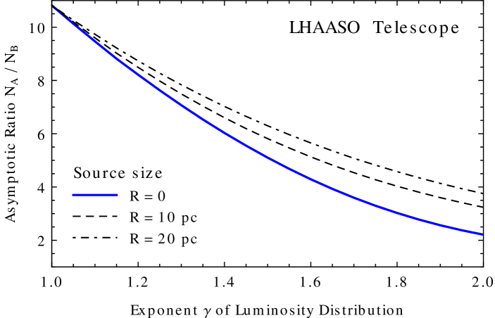
Figure 9: The ratio $N_{A}/N_{B}$ between the number of sources observed in region A and region B of an EAS telescope takes a asymptotic value when the sources have a very high absolute luminosity. This asymptotic ratio depends on the space, luminosity and size distribution of the sources. The figure shows the asymptotic ratio calculated for the cylindrically symmetric space distribution discussed in section A.1, sources of identical linear size $R$, and a luminosity distribution with the power–law with exponential cutoff form of Eq.(15), The asymptotic ratio is plotted as a function of the power–law slope $\gamma$, and three values of the source size ($R=0$, 10 and 20 pc). For a larger exponent $\gamma$ the number of faint sources increases, and the asymptotic ratio decreases.

The asymptotic ratio decreases for larger values of $\gamma$ because the relative importance of sources at large distances is suppressed. This effects is shown in Fig. 9 that plots the asymptotic ratio $N_{A}/N_{B}$ (for the LHAASO telescope) as a function of the exponent $\gamma$. The two curves in the figure are for point–like objects and for sources with a linear size of 20 pc. For the same luminosity distribution, the ratio $N_{A}/N_{B}$ becomes larger when the sources are more extended in space. This is a simple consequence of the fact that sources of large angular extension require a larger flux to be resolved.

The effect we have described is important, because the measured ratio of the number of resolved sources in different parts of the Galaxy can be compared with predictions based on the power–law assumptions for the luminosity distributions, obtaining an upper limit on the exponent $\gamma$.

V Interpretation of the HAWC and LHAASO gamma–ray observations

The main results of our study are contained in four tables (Tables 3–6) that list properties of the Galactic gamma–ray sources estimated from the data in the HAWC, LHAASO–WCDA, LHAASO–KM2A and LHAASO–KM2A-high catalogs, using the method outlined in section IV. These catalogs list sources observed in the energy intervals [1,10] TeV (for HAWC and LHAASO–WCDA), [25,100] TeV (for LHAASO–KM2A) and [10²,10³] TeV (for LHAASO–KM2A-high), and the estimated luminosities are integrated in the same energy intervals.

The relation between the luminosity of a source and its flux also depends on the spectral shape. In this study we made the simplifying assumption the all sources have the same spectral shape that is a approximated by a power–law of slope $\alpha=2.5$ in the [1,10] TeV energy interval, and $\alpha=3.25$ in the [25,100] TeV and and [10²,10³] TeV intervals. For a discussion of the motivation (and the limitations) of these choices see our companion paper lv_spectral_shapes .

The results in the tables are shown for four models of the Galactic gamma–ray sources. Two of the models assume identical point–like sources, but use the two forms for their space distribution described in Appendix A. In the other two models the luminosity distribution of the sources has the power–law form of Eq. (15) with exponent $\gamma=1.25$. In one case the sources are point–like, in the other they have a linear size of 20 pc. The choice of $\gamma=1.25$ is motivated by the fact that larger exponents are disfavored, because they predict too small $N_{A}/N_{B}$ ratios (see Fig. 9).

The first step of our study is to interpret the number of resolved sources in the two sky regions A and B in order to obtain estimates of $L_{0}$ (or $L_{*}$) and $L_{\rm tot}$ for the hypothesis of identical sources or a power–law luminosity distribution. Our analysis method is essentially geometrical, and therefore in the tables we also give the horizon for the resolution of a point–like source of luminosity $L_{0}$ (or $L_{*}$) with celestial declination $\delta=\lambda$, with $\lambda$ the geographic latitude of the telescope. Points in the sky with this declination culminate at the zenith, and for them the sensitivity is best, and the horizon is largest. The horizon for other directions can be be obtained using the curves in Fig. 3 and Eq. (9).

For the hypothesis of identical sources, the estimated value of the horizon $D_{H}(L_{0})$ is of the order of $\approx 10$ kpc for all catalogs, indicating that the sources can be resolved in a large, but limited fraction of the Milky Way volume. The result that the horizon is approximately the same for sources observed in different energy intervals can be understood by noting that the measured $N_{A}/N_{B}$ ratios are similar in all catalogs. This implies that for higher energy intervals the luminosity of the sources and the minimum flux for source resolution decrease at the same rate.

For the hypothesis of a power–law distribution, the estimated horizon $D_{H}(L_{*})$ is larger (on the order of 20–40 kpc), indicating that sources wih luminosities $L\gtrsim L_{*}$ can be resolved in most of the Galactic volume, however the population of Galactic sources contains many fainter objects that can only be resolved at shorter distances, reducing the measurable $N_{A}/N_{B}$ ratio. When the sources have a large linear size, the number of resolved nearby objects is reduced because they have a larger angular extension and require a higher flux. Accordingly the $N_{A}/N_{B}$ ratio is obtained with a smaller luminosity $L_{*}$ and a shorter horizon $D_{H}(L_{*})$.

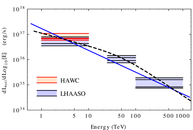
Figure 10: Total luminosity of the Galactic gamma–ray sources estimated from the sky distribution of resolved objects. The lines show the estimates obtained using the models of the source distributions also used to compute the results shown in Tables 3–6. The lines are not fits, but simple descriptions of the results. The solid line is a power–law of form $dL_{\rm tot}/d\log E\propto E^{-0.86}$). The dashed line is a broken power–law data with slopes 0.5 and 1.25 below and above a break energy of 50 TeV.

Fig.10 summarizes all the results on the estimate of the total luminosity of the Galactic sources $L_{\rm tot}$, showing them in the form $dL_{\rm ltot}/d\log_{10}E$. The figure shows that the uncertainty on the total luminosity is rather small, which is the consequence of a cancellation effect, because the total Galactic luminosity is the product of the source density and the average luminosity of the sources, and the number of observed resolved sources can be reproduced by a large density of faint sources visible in a small volume, or by a smaller density of brighter sources that can be resolved in a larger volume.

In fig.10 one of the two curves is a simple power–law of form:

$$\frac{dL_{\rm tot}}{d\log_{10}E}\approx 1.7\times 10^{37}~\left(\frac{E}{\rm TeV}\right)^{-0.86}~\frac{\rm erg}{\rm s}~,$$ (22)

and the second is a smoothly broken power–law with slopes of 0.50 and 1.25 below and above a break of width $w=0.60$:

$$\frac{dL_{\rm tot}}{d\log_{10}E}\approx 1.1\times 10^{37}~\left(\frac{E}{\rm TeV}\right)^{-0.50}~\left[1+\left(\frac{E}{50~{\rm TeV}}\right)^{1/w}\right]^{-0.25\,w}~\frac{\rm erg}{\rm s}~.$$ (23)

The pair of parameters $\{L_{0},L_{\rm tot}\}$ or $\{L_{*},L_{\rm tot}\}$ determine the luminosity distribution, and therefore it becomes possible to compute, for any region of the sky, the expected number of resolved sources, and also the total resolved and unresolved fluxes due to the sources. It is particularly interesting to obtain these estimates for those regions of the sky where measurements of the diffuse gamma–ray flux have been obtained, making it possible to compare the estimates with the observations.

Tables 3–6 report for each catalog, in all relevant regions of the sky: the calculated number of resolved sources, the fluxes of resolved and unresolved sources, and the ratio of the latter to the total source flux. The calculated unresolved source flux can then be compared with the measured diffuse flux, to estimate the fraction of the measured diffuse flux that should be attributed to the contribution of unresolved sources.

In fact, we estimated this unresolved sources contribution in two different ways. The first one is simply to compute the ratio $\Phi_{\rm unresolved}^{\rm model}/\Phi_{\rm diffuse}^{\rm data}$. In this way, the absolute value of the calculated unresolved flux is used. A second method is to estimate the unresolved flux from the sum of the fluxes of all resolved sources in the considered sky region ($\Phi_{\rm resolved}^{\rm data}$) multiplying by the calculated ratio $\Phi_{\rm unresolved}^{\rm model}/\Phi_{\rm resolved}^{\rm model}$. This method has the advantage that the effects of an imprecise description of the detector sensitivity (which determines the absolute value of the calculated fluxes) to a good approximation cancel out. The two methods are in reasonably good agreement with each other.

It should be noted that the estimates obtained with the models are calculated with numerical integrations that implicitly assume that the sources are smoothly distributed in space, neglecting the fact that they are discrete. The results of the calculation should therefore be considered as averages over all possible configurations of the Galaxy associated with the same underlying model. The fluctuations are to a good approximation Poissonian for the number of resolved sources, but can be much larger for the estimate of the resolved source flux, since the flux of an individual object is very sensitive to its distance from the Solar system (diverging at short distances $\propto D^{-2}$).

For the lowest energy interval ([1,10] TeV), the contribution of unresolved sources to the diffuse flux in the region where HAWC has measured the diffuse flux can reach large values ($\gtrsim 50$%) only for a power–law luminosity distribution and for sources of large linear size (20 pc), while in the other cases it remains significant but subdominant, accounting for a fraction of 15–30%.

The LHAASO catalog contains a list of sources identified in the [1,10] TeV energy range, and the data can be analysed with the methods discuss above to estimate the parameters of the source luminosity distribution $\{L_{0},L_{\rm tot}\}$ or $\{L_{*},L_{\rm tot}\}$, with results that are in good agreement with those obtained from the observations of HAWC (see tables 3 and 4. Table 4 gives estimates of the unresolved source flux in the Inner and Outer–Galaxy sky regions, however the LHAASO collaboration has not yet released measurements of the diffuse flux in this energy range.

At higher energies (in the [25,100] TeV and [10²,10³] TeV intervals), the results of the models can be compared with the LHAASO measurements of the diffuse flux in the Inner and Outer–Galaxy sky regions. It turns out that in the Outer–Galaxy region the contribution of unresolved sources to the diffuse flux is most likely subdominant. In the [25,100] TeV interval, this fraction is in most cases of the order of 10–30% of the observed flux, and can approach 50% or more only if the sources have large size.

The contribution of unresolved sources becomes significantly smaller in the higher energy interval [10²,10³] TeV, reflecting the fact that the resolved gamma–ray sources have a very soft spectral shape in this energy range.

For the Inner–Galaxy, in the [25,100] TeV energy range, the contribution of unresolved sources could account for a very large fraction ($\gtrsim 50$%) or even most of the observed diffuse flux. It should be noted, however, that the unresolved source fluxes calculated in this work refer to the entire sky region considered, without taking into account the masking adopted in the LHAASO measurement of the diffuse flux. If we tentatively assume that the diffuse flux at high energies has the same angular dependence as measured by Fermi–LAT at $E\simeq 10$ GeV, the correction factor (see Table 2) is of the order of 1/0.622, and the contribution of unresolved sources is reduced accordingly.

As in the case of the Outer–Galaxy, the contribution of unresolved sources to the diffuse flux is reduced in the highest energy interval [10²,10³] TeV, reflecting the softness of the spectra of the observed sources, and in most models accounts for a fraction of the order of $\sim 20$–30% of the observed diffuse flux.

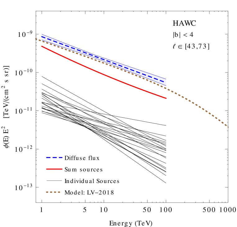
Figure 11: The shaded area shows the best fit and one sigma uncertainty for the diffuse gamma–ray flux measured by HAWC HAWC:2023wdq in the sky region {$|b|<4^{\circ}$, $43^{\circ}\leq\ell<73^{\circ}$. The thick red line shows the sum of the fits to the 21 sources in the HAWC third catalog HAWC:2020hrt that are in the same sky region, while the thin lines show the fits to the individual sources. In the plot the fits to the sources (and their sum) are divided by the solid angle $\Delta\Omega$ of the region to obtain an average flux. The thick dotted line is the prediction of the factorized model in LV–2018 Lipari:2018gzn .

A visualization of the relationship between the diffuse flux and the flux of the resolved sources for the HAWC and LHAASO catalogs is shown in figures 11 and 12. Fig. 11 shows the diffuse flux measured by HAWC in the sky region {$|b|<4^{\circ}$, $43^{\circ}\leq\ell\leq 73^{\circ}$}, together with the fits to all 21 sources resolved in the same region and the sum of all these fits. Integrating in the 1–10 TeV energy range, the observed diffuse flux is $\Phi_{\rm diff}\simeq(3.82^{+0.55}_{-1.10})\times 10^{-11}$  [cm^-2s^-1], while the flux of the resolved sources $\Phi^{\rm resolved}_{\rm sources}\simeq 1.94\times 10^{-11}$  [cm^-2s^-1], is about half as large. The study of the distribution of the sources resolved by HAWC suggests [see table 3] that most (50–80%) of the source flux in the region under study is due to contributions from resolved objects, so one can conclude that unresolved sources account for less than half of the measured diffuse flux. Fig. 11 also shows the prediction of the interstellar emission flux of the factorized model in LV–2018 Lipari:2018gzn which is in reasonably good agreement with the observed flux. Note that in HAWC:2023wdq the HAWC Collaboration compares the diffuse flux data with the DRAGON base model, which is smaller than the data by a factor of two.

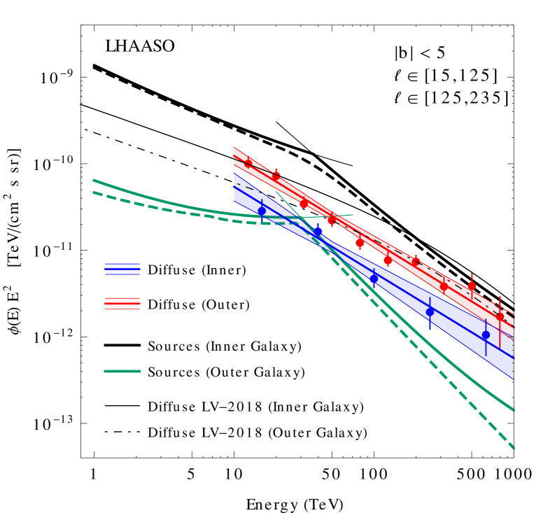
Figure 12: The shaded areas shows the measurements of the diffuse gamma–ray flux obtained by LHAASO LHAASO:2023gne in the sky regions {$|b|<5^{\circ}$, $15^{\circ}\leq\ell\leq 125^{\circ}$} (Inner–Galaxy), and {$|b|<5^{\circ}$, $125^{\circ}\leq\ell\leq 235^{\circ}$} (Outer–Galaxy). The thick lines show the sum of the fits of all sources listed in the 1st LHAASO catalog LHAASO:2023rpg in the two regions. The thick dashed lines show the sum of the combination of fits to the sources observed by both the WCDA and KM2A arrays. The thin lines show the predictions of the factorized model in LV-2018 Lipari:2018gzn for the two regions.

Fig. 12 shows the diffuse fluxes measured by LHAASO in the Inner and Outer–Galaxy regions, together with the fits to the sources resolved in these regions, and the sums of all the fits. In the Inner–Galaxy region 49 sources are measured by WCDA and 55 by KM2A, with 41 sources measured by both detector arrays, while in the Outer–Galaxy region 9 sources are measured by WCDA and 13 by KM2A with 7 measured by both arrays.

Comparison of these results shows that in the Outer–Galaxy the cumulative flux of the sources is approximately equal to the measured diffuse flux at $E\approx 30$ TeV, and then decreases more rapidly with energy. The estimates shown in Tables 5 and 6 suggest than the flux of unresolved sources is only a fraction of the combined flux of the resolved sources, and therefore most of the observed diffuse flux in this region is generated by interstellar emission, with the fraction of unresolved sources decreasing with energy because of their softer spectrum.

In the Inner–Galaxy region the combined flux of all resolved sources is larger than the measured diffuse flux. Note, however, that the diffuse flux is measured in only a fraction of the selected region due to masking of known sources. As discussed above, the solid angle after the masking has a larger $\langle|b|\rangle$ than the entire region, and therefore has also a smaller average flux. Taking into account this effect (a correction estimated of the order of 60% in Table 2), the diffuse flux and the resolved source flux are approximately equal in the [25,100] TeV energy range, and the diffuse flux becomes larger at higher energies. The results shown in Tables 5 and 6 then suggest that unresolved sources contribute a large fraction of the diffuse flux below 100 TeV, but become subdominant at higher energies.

VI Galactic Neutrino flux

It is well known that the emissions of gamma–rays and high energy neutrinos are intimately related, and that the simultaneous study of the fluxes of photons and neutrinos is of fundamental importance to understand the emission mechanisms and the properties of their sources.

Gamma–rays can be produced by the leptonic and hadronic mechanisms. In the first case the emission is generated by the radiation of relativistic electrons and positrons (via Compton scattering on radiation fields and/or Bremsstrahlung in interactions with ordinary matter) and in this case there is no corresponding neutrino emission. In the hadronic mechanism the gamma–rays are emitted in the decay of mesons created in the inelastic interactions of relativistic protons and nuclei, with the dominant source being the decay of neutral pions ($\pi^{0}\to\gamma\gamma$). For the hadronic mechanism the gamma–ray emission is accompanied by the emission of neutrinos generated in the Weak decays of mesons created in the same hadronic collisions. The main neutrino source is the chain decay of charged pions ($\pi^{+}\to\mu^{+}\nu_{\mu}$ followed by $\mu^{+}\to e^{+}\nu_{e}\overline{\nu}_{\mu}$ and charge conjugate modes). The neutrino flavors are modified during propagation due to oscillations, so that, assuming that charged pion decay is the primary production mechanism, the neutrinos that reach the Earth are to a first approximation a combination with equal weights of the three flavors (see Lipari:2007su for more discussion).

The production of charged and neutral pions is related by isospin symmetry and the pions decay spectra are well known, therefore it is possible to find a simple relation connecting the gamma–rays and neutrino emissions. The spectra of the final state particles generated in the decay of ultrarelativistic parents have a scaling form and depend only on the ratio of the energies of the decay product and the parent particle. The exact forms of the spectra of particles generated in pion decay are known, but for the discussion here it is an acceptable approximation to use the simple expressions:

$$\left.\frac{dN}{dx}\right|_{\pi^{0}\to\gamma}=2~\delta\left[x-\frac{1}{2}\right]$$ (24)

(with $x=E_{\gamma}/E_{\pi}$) for gamma–rays, and summing over all $\nu$ and $\overline{\nu}$ flavors:

$$\left.\frac{dN}{dx}\right|_{\pi^{\pm}\to\nu}=3~\delta\left[x-\frac{1}{4}\right]~$$ (25)

(with $x=E_{\nu}/E_{\pi}$) for neutrinos. Assuming that the spectra of the parent charged and neutral pions have the same shape and relative normalizations $R_{\pm}$ and $R_{0}=1-R_{\pm}$, it is then elementary to derive a simple relation between the neutrino and gamma–ray emissions. Neglecting absorption effects, the gamma–ray and neutrino fluxes are then related by:

$$\begin{array}[]{l}\phi_{\gamma}(E_{\gamma})=\phi_{\gamma}^{\rm lept}(E_{\gamma})+\phi_{\gamma}^{\rm had}(E_{\gamma})\\[9.95863pt] \phi_{\nu}(E_{\nu})\simeq(R_{\pm}/R_{0})\;3\;\phi_{\gamma}^{\rm had}\left(2\,E_{\nu}\right)\simeq 6\,\phi_{\gamma}^{\rm had}\left(2\,E_{\nu}\right)\end{array}$$ (26)

where in the last equality we have assumed the ratio $R_{\pm}/R_{0}=2$ predicted by isospin symmetry. This equation states the well known fact that if the gamma–ray flux is generated by the hadronic mechanism, it is accompanied by a neutrino flux of similar magnitude, because in the second line of Eq.(26) the factor of six compensates for the fact that neutrinos are produced at an energy lower by a factor of two, with spectra that fall off rapidly with energy. Conversely, a neutrino flux (generated by the standard mechanism described above) is always accompanied by a gamma–ray flux of comparable magnitude.

In the presence of absorption, the observable fluxes of gamma–rays are reduced, however absorption during propagation is small or negligible for energy below 1 PeV Vernetto:2016alq , and absorption inside the sources is also expected to be small in current models of Galactic objects. By comparing the gamma–rays and neutrino fluxes, it is therefore in principle possible to determine the relative importance of the hadronic and leptonic emission mechanisms.

The Galactic neutrino flux observed by IceCube is the sum of a diffuse component due to interstellar emission and a second component due to the sum of all neutrino sources. The only difference with respect to the gamma–ray case [see Eq. (11)] is that until now no Galactic neutrino sources have yet been identified.

It is expected that at high energies the interstellar emission is dominated by the hadronic mechanism, and therefore produces approximately equal fluxes of neutrinos and gamma–rays. The nature of the mechanisms that operate in the high energy sources is an object of debate. In some classes of sources, such as Pulsar Wind Nebulae (PWN), the main emission mechanism is very likely leptonic, but it is possible (and in some sense also inevitable) that the Galaxy contains sources that generate gamma–rays and neutrinos via the hadronic mechanism. This important question can be addressed comparing the gamma–ray and neutrino fluxes.

VI.1 The IceCube evidence for Galactic neutrino emission

Recently the IceCube collaboration published IceCube:2023ame evidence for the emission of high energy neutrinos from the Galactic plane in the approximate energy range from 1 to 100 TeV. This result was obtained by using machine learning techniques and comparing, over the entire celestial sphere, the IceCube data with three different templates for the diffuse neutrino flux and with a background–only hypothesis, leaving the absolute normalization of the templates as a free parameter. This study lead to evidence for the existence of a Galactic neutrino flux at the level of 4.71, 4.37 and 3.96 $\sigma$’s for the three templates IceCube:2023ame .

One of the three templates (the $\pi^{0}$ model) is a phenomenological one, based on the angular distribution of the diffuse gamma–ray flux measured by the Fermi–LAT (for $E\lesssim 1$ TeV) Fermi-LAT:2012edv and extrapolated to higher energies with a simple $\propto E^{-2.7}$ spectrum, assuming factorization of the energy and angular dependencies of the flux. The other two models (KRA${}_{\gamma}^{5}$ and KRA${}_{\gamma}^{50}$) are based on predictions of the diffuse gamma–ray flux constructed using the cosmic ray transport software package DRAGON including a radially dependent diffusion coefficient for cosmic–ray propagation. This results in a harder spectrum for particles near the center of the Galaxy ($\propto E^{-2.5}$ in the energy range of the Icecube observations), and in an angular distribution becomes progressively more concentrated toward the Galactic Center with increasing energy. The superscripts in the template names indicate the cutoff energies (5 and 50 PeV) of the cosmic ray proton spectrum at Earth.

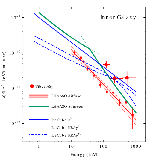
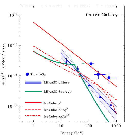
Figure 13: Comparison of the average Galactic gamma–ray and neutrino fluxes obtained by Tibet–AS$\gamma$ TibetASgamma:2021tpz , LHAASO LHAASO:2023rpg ; LHAASO:2023gne and IceCube IceCube:2023ame . The IceCube results are shown in the form of gamma–ray fluxes calculated with Eq.(26) and using as input the neutrino fluxes shown in Fig.S8 of IceCube:2023ame . These neutrino fluxes are the three templates averaged over the Tibet–AS$\gamma$ Inner and Outer Galaxy regions with the absolute normalization obtained from best fits to the data over the entire celestial sphere. The top (bottom) panel shows the IceCube results for the Inner–Galaxy (Outer–Galaxy) region, together with the measurements of the Tibet–AS$\gamma$ and LHAASO telescopes. Note that the definitions of the sky regions differ for the two gamma–ray telescopes. see Table 2).

It is not easy to compare the IceCube neutrino results (based on all sky templates of the neutrino flux) with those of the gamma–ray telescopes (that measure the flux in some limited regions of the sky). However, the supplemental material of the IceCube paper IceCube:2023ame shows (in Fig.S8) the spectra of the three templates (with the best fit normalization) averaged over the Tibet–AS$\gamma$ Inner and Outer–Galaxy regions. These spectra, transformed into gamma–ray spectra using Eq.(26) are shown in Fig. 13 together with the Tibet–AS$\gamma$ and LHAASO telescopes measurements. Examining this figure, several comments are in order:

[A] The average fluxes measured by Tibet–AS$\gamma$ TibetASgamma:2021tpz and LHAASO LHAASO:2023rpg ; LHAASO:2023gne in their respective Inner–Galaxy regions are expected to be very similar to each other, because the LHAASO region is larger (the two regions have the same latitude range $|b|\leq 5^{\circ}$, but longitude ranges $15^{\circ}\leq\ell\leq 125^{\circ}$ for LHAASO versus $25^{\circ}\leq\ell\leq 100^{\circ}$ for Tibet–AS$\gamma$) but the extension is partly toward the Galactic Center and partly toward the Galactic anti–center. The total gamma–ray flux observed by LHAASO in this sky region is dominated by the contribution of photons emitted by identified sources. Summing the resolved source contribution with the measured diffuse flux, and correcting for the effect of the masking [see Table 2] the LHAASO total gamma–ray flux can be reconciled with the flux measured by Tibet–AS$\gamma$. Note however that this conclusion requires the assumption that, contrary to what is discussed in TibetASgamma:2021tpz , most of the gamma–ray flux observed by the Tibet–AS$\gamma$ telescope is due to the contribution of unresolved sources.

[B] The Outer–Galaxy regions for Tibet–AS$\gamma$ and LHAASO are quite different, because the one for Tibet–AS$\gamma$ extends to smaller longitudes ($50^{\circ}\leq\ell\leq 200^{\circ}$ versus $125^{\circ}\leq\ell\leq 235^{\circ}$ for LHAASO. For LHAASO, according to the analysis presented in the previous section, the total gamma–ray flux in the Outer–Galaxy region consists of approximately equal contributions from sources and interstellar emission, with the latter dominating the flux observed as diffuse. In the flux measured by Tibet–AS$\gamma$ the contribution of sources is estimated to be larger than for LHAASO, with the interstellar emission accounting for a fraction of the order of 25% of the total flux.

[C] The crucial question that can be addressed by comparing the gamma–ray and neutrino fluxes, is what fraction of the gamma–ray emission from the sources is produced by the hadronic mechanism, and therefore accompanied by neutrinos. The high neutrino flux observed in the Tibet–AS$\gamma$ Inner–Galaxy region for a neutrino energy of the order of 50 TeV (gamma–ray energy of the order of 100 TeV) is an intriguing hint that an important fraction of the source emission could be generated by the hadronic mechanism, but a robust conclusion requires a more in depth study.

[D] The $\pi^{0}$ and the two KRA$\gamma$ templates have two main differences, with the KRA$\gamma$ templates predicting: (i) much harder spectra in directions toward the Galactic Center, and (ii) a significantly larger Inner/Outer ratio. The gamma–ray observations find spectra that are soft and have a shape independent of direction. For example, the diffuse flux measurements of LHAASO above 25 TeV were fitted with power–law spectra of equal slopes ($2.99\pm 0.08$ and $2.99\pm 0.14$) in the Inner and Outer Galaxy. In addition, the observed Inner/Outer ratios (for both Tibet–AS$\gamma$ and LHAASO are smaller than the predictions of the KRA$\gamma$ templates. Accordingly, the hypothesis at the basis of the KRA$\gamma$ models seems to be disfavored.

VII Summary and Outlook

The study of the Galactic diffuse gamma–ray flux is of great importance, since the flux encodes information about the cosmic ray spectra in different regions of the Milky Way, and the extension of the measurements to very high energies in the TeV and PeV energy ranges is of crucial importance. However, in order to interpret the recent observations of high energy telescopes it is necessary to identify and subtract the contribution of unresolved sources to what is measured as a diffuse flux. The measurement of the unresolved source flux is of course also of great importance in itself and is required for a complete understanding of the properties of the Galactic high energy accelerators.

The recent publications of LHAASO LHAASO:2023gne and HAWC HAWC:2023wdq , which have reported measurements of the diffuse flux in some regions of the Galactic disk, note in the discussion of their results that the data appear to show a significant excess over theoretical expectations that can be explained as the contribution of unresolved objects.

However, the evidence for the existence of an excess in the diffuse gamma–ray flux at high energies is based on the comparison of the data with some specific theoretical models, while other models predict larger fluxes. For example, in this work we have shown that the predictions of the LV–2018 model Lipari:2018gzn are in reasonably good agreement with the HAWC and LHAASO observations, and are in fact somewhat larger than the LHAASO data (see also Vecchiotti:2024kkz ). Therefore the size of the contribution of unresolved sources to the observed diffuse gamma–ray flux remains a very important open problem that can be addressed in several ways.

The approach followed in this paper is based on the study of the angular distributions of the resolved sources. These distributions are determined in part by the (direction dependent) sensitivity of the telescopes but also encode the space and luminosity distributions of the Galactic gamma–ray sources. A sufficiently accurate description of these distributions allows the fluxes of unresolved sources to be calculated. In this paper, to extract this information from the data, we make two main simplifying assumptions: (i) that the space and luminosity distributions of the Galactic gamma–ray sources are factorized, and (ii) that their space distribution is known, at least to a reasonably good approximation. With these assumptions it is possible to infer the parameters of the luminosity distribution of the Galactic gamma–ray sources from the measured angular distribution of those that are resolved, and then to compute the unresolved source flux for any region of interest. It is important to note that this program does not require any measurement of the distances of the resolved sources.

Two major difficulties are that the total number of resolved sources is still relatively small, and that the detailed form of the sky distribution of the sources is not known very precisely. In fact the angular distribution of the resolved sources is determined by the spiral structure of the Milky Way, and by the shape of the spiral arms in the vicinity of the Earth. Current models of the spiral structure cannot describe the details of the longitude and latitude distributions of the data. On the other hand, the general structure of the space distribution of the sources, i.e. a thin disk with a density decreasing exponentially with galactocentric radius is reasonably well known. For these reasons, in this paper we have performed a first approximation study, by dividing the sky into two regions of equal solid angle and sensitivity, one centered (to a good approximation) on the Galactic anticenter (region B), and the other as close as possible to the Galactic center (region A), and comparing the number of resolved sources in the two regions. In this way the statistical errors are reduced, and the uncertainties in the description of the space distribution of the sources play a less important role. Of course, this choice has the important limitation that it allows to determine only two parameters for the luminosity distribution of the sources, which can be chosen as the total luminosity of the ensemble of all Galactic sources, and a characteristic luminosity for the individual sources.

The LHAASO and HAWC catalogs observe 3–4 times more sources in the sky region A toward the Galactic center. Since the density of stars and other astrophysical objects, changes with the galactocentri radius only on a scale of several kpc, it is easy to see that the large $N_{A}/N_{B}$ ratio implies that gamma–ray sources can be resolved out to distances of several kpc. In addition, this result allows to place limits on the contribution of very faint objects to the unresolved source flux. This is because faint objects can only be resolved at short distances, and if they were too numerous, they would push the ratio $N_{A}/N_{B}$ down toward unity.

In this work we have used a model of the source luminosity distribution that is a power–law with an exponential cutoff, and found that the observation of a large asymmetry in the number of resolved sources in the regions A and B can be used to set an upper limit on the exponent that controls the low luminosity end of the distribution $\gamma\lesssim 1.25$.

We have used the ratio $N_{A}/N_{B}$ in the LHAASO and HAWC catalogs to estimate the horizon for source resolution, and thus the luminosity of the individual gamma–ray sources, and then we used the absolute numbers of resolved sources to estimate the total luminosity of all Milky Way sources. This total luminosity can be reconstructed with an uncertainty of about a factor of two, and (in units erg/s) is approximately $1.5\times 10^{37}$, $4\times 10^{36}$ and $4\times 10^{35}$ in the energy intervals [1,10], [10,100], and [10²,10³] TeV.

These results were then used to estimate the flux of unresolved sources, and it was found that, with the possible exception of directions close to the Galactic Center, the contribution of unresolved sources is likely to be subdominant in what is measured as the diffuse gamma–ray flux. The simplest way to obtain a first estimate of the unresolved source flux is to use the measured flux of the resolved sources, and to note that if the horizon for source resolution is of the order of $\approx 10$ kpc, the flux from sources beyond the horizon is only a fraction of the flux from the sources inside the horizon.

More detailed studies of the properties of the Galactic gamma–ray sources are not only desirable but in fact necessary to verify the results and conclusions obtained in the simple study developed here. A more precise description of the spiral structure of the Milky Way, capable of reproducing the observed features in the latitude and longitude distributions of the sources is very desirable, and would allow the shape of the luminosity distribution of the sources to be studied in more detail. In would also be very interesting to perform separately these studies for different classes of sources, which are also likely to have different extensions. It is also clear that the inclusion in future studies of the available information on the distances for a subset of the sources would be very valuable.

Acknowledgments We are grateful to Cao Zhen, Felix Aharonian, You Zhi Yong, Xi Shao Qian and Zha Min for useful discussions.

Appendix A Space distribution of the Milky Way gamma–ray sources

A.1 Cylindrically symmetric model

In this work to describe the space distribution of the Milky Way sources we will use a simple form symmetric for rotations around the $z$ axis and for reflections on the ($xy$) Galactic plane:

$$f(\vec{x})=f_{r}(r)\,f_{z}(z)$$ (27)

For the radial part we used the form introduced by Yusifov and Kucuk Yusifov:2004fr and then used by several other authors:

$$f_{r}(r)=K_{r}~\left(\frac{r+r_{0}}{r_{\odot}+r_{0}}\right)^{a}~\exp\left[-\beta\left(\frac{r-r_{\odot}}{r_{\odot}+r_{0}}\right)\right]$$ (28)

This form depends on three parameters ($r_{0}$, $a$ and $\beta$) with $K_{r}$ is a normalization factor that can be calculated numerically.

For the $z$ dependence we used an exponential form, with a correction to avoid a discontinuity in the derivative at $z=0$:

$$f_{z}(z)=K_{\zeta}~e^{z/Z}\left(1+e^{2z/(Z\,\zeta)}\right)^{-\zeta}$$ (29)

with $K_{\zeta}$ a normalization factor (to insure normalization to unity):

$$K_{\zeta}=\frac{1}{Z}\;\frac{4\Gamma(\zeta)}{\zeta\,\Gamma^{2}(\zeta/2)}\simeq\frac{1}{Z}\;\left(1+\frac{\pi^{2}\zeta^{2}}{24}+\ldots\right)~.$$ (30)

In the limit of $\zeta\to 0$ one has $f_{z}(z)\to e^{-|z|/Z}/Z$, and the function has a cusp at $z=0$, while for $\zeta=1$ one has $f_{z}(z)=[\pi\,Z\,\cosh(z/Z)]^{-1}$. In general the second derivative of $f_{z}(z)$ at $z=0$ is:

$$\left.\frac{d^{2}f_{z}(z)}{dz^{2}}\right|_{z=0}=-\frac{1}{\zeta\,Z^{2}}~.$$ (31)

For our numerical studies we have tested several set of values for the parameters, but the results we are presenting are based on the parameters suggested by Lorimer et al.Lorimer:2006qs to describe the observations of the Parkes 20-cm multibeam pulsar survey of the Galactic plane ($r_{0}=0.55$ kpc, $a=1.64$, $\beta=4.01$) for the radial distribution and $Z=0.18$ kpc for the $z$ distribution.

A.2 Spiral model of the Milky Way

Our model for the spiral structure of the Galaxy is based on the analysis by Reid et al. Reid:2019 of trigonometric parallax and proper motion measurements of molecular masers associated with very young high-mass stars. These objects trace the high-mass star-forming regions of our Galaxy, where gamma ray sources such as PWN and SNR are more likely to be found. The maser measurements have been performed in the 1^st, 2^nd and 3^rd Galactic quadrants. Considering also the well-established arm tangencies in the 4^th Galactic quadrant, the authors developed a model with four spiral arms and some extra arm segments and spurs. Each arm $k$ is described by a logarithmic spiral curve:

$$r=R_{k}\;\exp\left[-(\beta-\beta_{k})\tan\psi_{k}\right]$$ (32)

where $r$ is the distance from the Galactic center, $\beta$ the azimuth angle and $\psi$ the pitch angle. The values of $\psi$, $R_{k}$ and $\beta_{k}$ parameters have been found by fitting the spiral function to the data. The best fit pitch angles are not constant along the spiral lines, but change at some azimuth angles. The best-fit parameter values are given in Table 1 of Reid et al. for a limited range of azimuth angles. Beyond this range we extracted them from Fig. 1 of the same paper, and we extrapolated the spiral lines outside the region shown in the figure using the same pitch angles of the last segment of the curve. In our model we consider four main arms: Norma–Outer, Scutum–Centaurus, Sagittarius–Carina and Perseus, plus the local Orion arm, a small spur in which the Sun is located.

Fitting the maser data, Reid et al. found that the arms width in the Galactic plane increases with the distance $r$ from the Galactic center and for $r>$ 3 kpc can be described by the expression:

$$w(r)=0.336+0.036\,(r-r_{\odot})$$ (33)

where $w(r)$ is in kpc and $R_{\odot}$ = 8.15 kpc.

Using this geometric model of the Galaxy, we have ”filled” the arms (projected on the Galactic plane) with a source number consistent with our model with cylindrical simmetry (described in Appendix A1), normalizing the source number of the two models for each distance $r>$ 4 kpc from the Galactic center. More explicitly, if there are $N$ spiral arms at the distance $r$, then each arm contains (between $r$ and $r+dr$) 1/$N$ of the number of sources located in the ring of area 2$\pi$ $rdr$ of the cylindrical model. The sources are then distributed on the Galactic plane, perpendicularly to each spiral line, according to the expression (33).

For the Galactic center region ($r<4$ kpc), we assume a bar structure with a source density (projected onto the Galactic plane) according to the long-bar model by Wegg et al. (Eq.9 in Wegg:2015 ):

$$\rho_{b}(x_{b},y_{b})\propto\exp\left\{-\left[\left(\frac{x_{b}}{X_{b}}\right)^{g}+\left(\frac{y_{b}}{Y_{b}}\right)^{g}\right]^{\frac{1}{g}}\right\}~G\left(\frac{r_{b}-R_{b}}{\sigma_{b}}\right)$$ (34)

where $x_{b}$ and $y_{b}$ are right-handed galactocentric coordinates with the $x_{b}$ axis oriented along the major axis of the bar, which is assumed to be inclined by 30 degrees with respect to the line connecting the Galactic center to the Sun and $r_{b}=(x_{b}^{2}+y_{b}^{2})^{1/2}$. $G(x)$ is a function describing the outer cutoff of the bar along the major axis: $G(x)$ = 1 for $x\leq$ 1, and $G(x)=\exp(-x^{2})$ for $x>$ k1. We assume no cutoff toward the Galactic center. According to Wegg:2015 , the values of the parameters are: $X_{b}$ = 3.05 kpc, $Y_{b}$ = 0.68 kpc, $g$ = 2.27, $R_{b}$ = 3.85 kpc and $\sigma_{b}$ = 0.72 kpc.

The source density of the bar is normalized by requiring that the total number of sources (spirals plus bar) be equal to the number of sources in the cylindrical model. The source density is adjusted to smoothly connect the bar to the spiral arms.

For the source distribution along the $z$ coordinate, we use (for spiral arms and bar) an exponentially decreasing density as $exp(-|z|/z_{0})$ with $z_{0}=0.18$ kpc, consistent with the previously described cylindrical model (except for the cusp correction, which is not applied here).

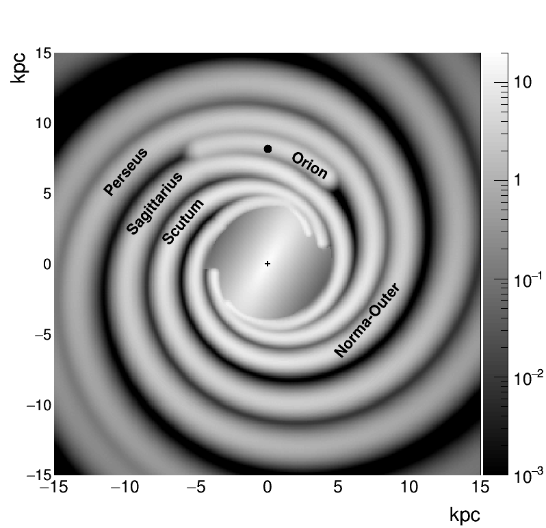
Figure 14: Model of the spiral structure of the Milky Way described in Appendix A.2. The position of the Solar System is indicated by the black dot.

Fig. 14 shows the source density of the model projected on the Galactic plane.

Table 3: Estimate of gamma–ray sources properties obtained from the observations of the HAWC telescope HAWC:2020hrt . The top part of the table lists information obtained by the telescope: the total number of resolved Galactic sources and the number of resolved sources in the sky regions A and B [defined in Eq. (3)]. More experimental results are given for a smaller sky region (the Inner–Galaxy region) where the HAWC Collaboration has obtained a measurement of the average diffuse flux: the number of resolved sources in the region, the best fit for the diffuse flux, and the total flux from resolved sources in the region. The bottom part of the table lists results obtained interpreting the data in the framework of some models discussed in this work, defined by the sources space and luminosity distributions and the source linear size $R$. The four columns are for four models. In the first two the Galactic sources are assumed to be point–like and identical, with luminosity $L_{0}$, but two different space distributions are used, one cylindrically symmetric, and one including a description of the spiral structure of the Milky Way [see Appendix A]. In the other two models the luminosity distribution of the sources is a power–law of index $\gamma=1.25$ with cutoff luminosity $L_{*}$ [see Eq. (15)]. The horizon listed in the table is the maximum distance to resolve a point–like source with celestial declination $\delta=\lambda$ and luminosity $L_{0}$ (for the identical sources model) or $L_{*}$ (for the power–law luminosity distribution models). The last two rows in the table compare the flux of unresolved sources estimated (with two different methods, see main text) in the model with the observed diffuse flux.

HAWC telescope. Energy Interval [1–10] TeV
All Sky: $N_{\rm sources}=63$     Regions A: $N_{A}=49$,     Region B: $N_{B}=14$.
Inner Galaxy [($|b|<4^{\circ}$), ($43^{\circ}\leq\ell\leq 73^{\circ})$]
$N_{\rm sources}^{\rm data}=21$
$\Phi_{\rm resolved}^{\rm data}=1.94\times 10^{-11}$  [cm-2s-1].
$\Phi_{\rm diffuse}^{\rm data}=(3.82^{+0.55}_{-1.10})\times 10^{-11}$  [cm-2s-1]
$\Phi_{\rm diffuse}^{\rm data}/\Phi_{\rm resolved}^{\rm data}=2.0^{+0.3}_{-0.6}$
Modeling of gamma–ray sources
	Model 1	Model 2	Model 3	Model 4
Luminosity distribution	Identical sources	Identical sources	P.L. ($\gamma=1.25$)	P.L ($\gamma=1.25$)
Space distribution	Smooth (PWN)	Spirals	Smooth (PWN)	Smooth (PWN)
Source size	$R=0$	$R=0$	$R=0$	$R=20$ pc
Global properties of Galactic gamma–ray sources
Horizon [kpc]	$6.6^{+1.9}_{-2.2}$	$7.7^{+2.0}_{-2.2}$	$13.9^{+8.7}_{-5.8}$	$9.9^{+5.5}_{-4.1}$
$L_{0}$ or $L_{*}$ [$10^{33}$ erg/s]	$6.4^{+4.2}_{-3.5}$	$8.5^{+4.1}_{-3.2}$	$24^{+44}_{-17}$	$14.3^{+20.}_{-9.3}$
$L_{\rm tot}$ [$10^{36}$ erg/s]	$5.8^{+0.31}_{-0.25}$	$7.0^{+0.32}_{-0.26}$	$6.6^{+1.9}_{-0.8}$	$10.8^{+3.9}_{-0.5}$
Modeling sources in Inner–Galaxy
$N_{\rm sources}^{\rm model}$	$17^{+2}_{-4}$	$23^{+2}_{-5}$	$15\pm 1$	$17^{+1}_{-3}$
$\Phi_{\rm resolved}^{\rm model}$ [$10^{-11}$ (cm2s)-1]	$2.2^{+0.5}_{-0.6}$	$3.3^{+0.6}_{-0.7}$	$2.7^{+1.3}_{-0.9}$	$3.4^{+0.7}_{-0.5}$
$\Phi_{\rm unresolved}^{\rm model}$ [$10^{-11}$ (cm2s)-1]	$0.91^{+0.49}_{-0.32}$	$0.95^{+0.50}_{-0.33}$	$0.91^{+0.50}_{-0.29}$	$2.23^{+2.53}_{-0.98}$
$f_{u}=\Phi_{\rm unresolved}^{\rm model}/\Phi_{\rm all}^{\rm model}$	$0.29^{+0.18}_{-0.11}$	$0.22^{+0.15}_{-0.12}$	$0.25^{+0.20}_{-0.12}$	$0.40^{+0.22}_{-0.16}$
$\Phi_{\rm unresolved}^{\rm model}/\Phi_{\rm diffuse}^{\rm data}$	$0.24^{+0.08}_{-0.12}$	$0.15^{+0.06}_{-0.12}$	$0.24^{+0.08}_{-0.12}$	$0.58^{+0.45}_{-0.33}$
$[\Phi_{\rm sources}^{\rm data}\,f_{u}/(1-f_{u})]/\Phi_{\rm diffuse}^{\rm data}$	$0.21^{+0.18}_{-0.12}$	$0.17^{+0.21}_{-0.09}$	$0.17^{+0.19}_{-0.11}$	$0.33^{+0.39}_{-0.21}$

Table 4: Estimate of gamma–ray sources properties obtained from the observations of the LHAASO-WCDA telescope LHAASO:2023rpg in the energy range [1,10] TeV. The structure of this table is the same as for table 3, with the top part listing experimental results, and the bottom part showing theoretical estimates obtained using the same models. Both experimental results and theoretical estimates are shown for the two sky regions (Inner–Galaxy and Outer–Galaxy regions) where LHAASO has published measurements of the diffuse flux in the higher energy range ($E>25$ TeV). A measurement of the diffuse flux in the WCDA energy range is not yet available at the moment.

LHAASO–WCDA telescope. Energy Interval [1–10] TeV
All Sky: $N_{\rm sources}=65$     Regions A: $N_{A}=51$,     Region B: $N_{B}=14$.
Inner Galaxy [($|b|<5^{\circ}$), ($15^{\circ}\leq\ell\leq 125^{\circ})$]
$N_{\rm inner}^{\rm data}=49$
$\Phi_{\rm resolved}^{\rm data}=25.8\times 10^{-11}$  (cm2s)-11.
Outer–Galaxy [($|b|<5^{\circ}$), ($125^{\circ}\leq\ell\leq 235^{\circ})$]
$N_{\rm outer}^{\rm data}=9$
$\Phi_{\rm resolved}^{\rm data}=1.38\times 10^{-11}$  (cm2s)-1].
Modeling of gamma–ray sources
	Model 1	Model 2	Model 3	Model 4
Luminosity distribution	Identical sources	Identical sources	P.L. ($\gamma=1.25$)	P.L ($\gamma=1.25$)
Space distribution	Smooth (PWN)	Spirals	Smooth (PWN)	Smooth (PWN)
Source size	$R=0$	$R=0$	$R=0$	$R=20$ pc
Global properties of Galactic gamma–ray sources
Horizon [kpc]	$9.2\pm 3.2$	$9.0^{+3.7}_{-2.5}$	$27.^{+49.}_{-15.}$	$20.^{+29.}_{-11.}$
$L_{0}$ or $L_{*}$ [$10^{33}$ erg/s]	$8.0^{+6.5}_{-4.5}$	$7.5^{+7.5}_{-3.5}$	$67.^{+90}_{-30}$	$38.^{+50.}_{-30.}$
$L_{\rm tot}$ [$10^{36}$ erg/s]	$4.3^{+0.9}_{-0.6}$	$3.5^{+1.2}_{-0.6}$	$6.7^{+11}_{-2.6}$	$7.9^{+5.4}_{-1.0}$
Modeling LHAASO–WCDA sources in Inner–Galaxy
$N_{\rm inner}^{\rm model}$	$44^{+4}_{-8}$	$43^{+4}_{-7}$	$43^{+4}_{87}$	$44^{+4}_{-8}$
$\Phi_{\rm resolved}^{\rm model}$   [$10^{-11}$ (cm2s)-1]	$6.4^{+2.3}_{-2.1}$	$7.1^{+3.5}_{-2.1}$	$11.4^{+15.}_{-6.1}$	$11.8^{+12}_{-4.5}$
$\Phi_{\rm unresolved}^{\rm model}$   [$10^{-11}$ (cm2s)-1]	$2.2^{+0.8}_{-0.5}$	$1.7^{+0.6}_{-0.6}$	$2.1^{+0.9}_{-0.7}$	$3.7^{+3.0}_{-2.0}$
$f_{u}=\Phi_{\rm unresolved}^{\rm model}/\Phi_{\rm all}^{\rm model}$	$0.25^{+0.15}_{-0.09}$	$0.20^{+0.12}_{-0.1-}$	$0.16^{+0.20}_{-0.12}$	$0.24^{+0.20}_{-0.16}$
Modeling LHAASO–WCDA sources in Outer–Galaxy.
$N_{\rm onner}^{\rm model}$	$10.0\pm 2.1$	$9.2^{+2/6}_{-1.5}$	$8.8^{+1.7}_{-1.3}$	$9.2^{+1.7}_{-1.4}$
$\Phi_{\rm resolved}^{\rm model}$   [$10^{-11}$ (cm2s)-1]	$3.3^{+0.7}_{-0.5}$	$4.2^{+1.4}_{-0.7}$	$5.1^{+8.7}_{-2.0}$	$5.2^{+4.7}_{-0.7}$
$\Phi_{\rm unresolved}^{\rm model}$   [$10^{-11}$ (cm2s)-1]	$0.18^{+0.19}_{-0.08}$	$0.16^{+0.09}_{-0.08}$	$0.28^{+0.22}_{-0.11}$	$0.54^{+0.64}_{-0.23}$
$f_{u}=\Phi_{\rm unresolved}^{\rm model}/\Phi_{\rm all}^{\rm model}$	$0.055^{+0.075}_{-0.029}$	$0.039^{+0.034}_{-0.023}$	$0.054^{+0.100}_{-0.042}$	$0.100^{+0.160}_{-0.073}$

Table 5: Estimate of gamma–ray sources properties obtained from the observations of the LHAASO–KM2A telescope LHAASO:2023rpg in the energy range [25,100] TeV. The structure of this table is the same as for table 3 and 4 with the top part listing experimental results, and the bottom part showing theoretical estimates obtained using the same models. Experimental results and theoretical estimates are given for the two sky regions (Inner–Galaxy and Outer–Galaxy region) where LHAASO has published measurements of the diffuse flux. Four rows compare the model estimates (obtained with two different methods, see main text) of the unresolved source flux in the two (Inner–Galaxy and Outer–Galaxy) regions with the measurements of the diffuse gamma–ray flux.

LHAASO–KM2A Telescope. Energy Interval [25,100] TeV
All Sky: $N_{\rm sources}=75$     Region A: $N_{A}=58$     Region B: $N_{B}=17$.
LHAASO Inner–Galaxy [($|b|<5^{\circ}$), ($15^{\circ}\leq\ell\leq 125^{\circ}$)
$N_{\rm sources}^{\rm data}=52$
$\Phi_{\rm resolved}^{\rm data}=11.9\times 10^{-13}$  [cm-2s-1].
$\Phi_{\rm diffuse}^{\rm data}=(3.12^{+0.42}_{-0.39})\times 10^{-13}$  [cm-2s-1]     (masking sources)
$\Phi_{\rm diffuse}^{\rm data}/\Phi_{\rm resolved}^{\rm data}=0.26\pm 0.03$
LHAASO Outer–Galaxy [($|b|<5^{\circ}$), ($125^{\circ}\leq\ell\leq 235^{\circ}$)]
$N_{\rm sources}^{\rm resolved}=10$
$\Phi^{\rm resolved}_{\rm sources}=1.53\times 10^{-13}$  [cm-2s-1]
$\Phi_{\rm diffuse}^{\rm data}=(1.38^{+0.29}_{-0.26})\times 10^{-13}$  [cm-2s-1]     (masking sources)
$\Phi_{\rm diffuse}^{\rm data}/\Phi^{\rm resolved}_{\rm sources}=0.90^{+0.19}_{-0.17}$
Modeling of gamma–ray sources
	Model 1	Model 2	Model 3	Model 4
Luminosity distribution	Identical sources	Identical sources	P.L. ($\gamma=1.25$)	P.L ($\gamma=1.25$)
Space distribution	Smooth (PWN)	Spirals	Smooth (PWN)	Smooth (PWN)
Source size	$R=0$	$R=0$	$R=0$	$R=20$ pc
Global properties of Galactic gamma–ray sources
Horizon [kpc]	$7.9^{+2.4}_{-2.5}$	$8.1^{+1.9}_{-3.2}$	$18.8^{+18.}_{-9.}$	$14.2^{+11.}_{-7.}$
$L_{0}$ or $L_{*}$ [$10^{32}$ erg/s]	$6.9^{+4.9}_{-3.7}$	$7.2^{+3.7}_{-4.6}$	$39^{+80}_{-29}$	$22.^{+49.}_{-16.}$
$L_{\rm tot}$ [$10^{35}$ erg/s]	$5.5^{+0.75}_{-0.60}$	$4.5^{+0.56}_{-1.3}$	$7.2^{+4.8}_{-1.9}$	$8.7^{+2.3}_{-0.5}$
Modeling LHAASO–KM2A Inner–Galaxy region
$N_{\rm Inner}^{\rm model}$	$49^{+5}_{-9}$	$48^{+5}_{-9}$	$48^{+5}_{-9}$	$48^{+5}_{-9}$
$\Phi_{\rm resolved}^{\rm model}$   [$10^{-13}$ (cm2s)-1]	$4.2^{+1.2}_{-1.2}$	$4.8^{+1.1}_{-2.1}$	$6.2^{+5.9}_{-2.7}$	$6.2^{+3.6}_{-1.9}$
$\Phi_{\rm unresolved}^{\rm model}$[$10^{-13}$ (cm2s)-1]	$1.9^{+0.6}_{-0.4}$	$1.5^{+0.4}_{-0.4}$	$1.9^{+0.6}_{-0.6}$	$3.3^{+2.4}_{-1.1}$
$f_{u}=\Phi_{\rm unresoled}^{\rm model}/\Phi_{\rm all}^{\rm model}$	$0.31^{+0.14}_{-0.09}$	$0.24^{+0.16}_{-0.08}$	$0.23^{+0.19}_{-0.13}$	$0.35^{+0.22}_{-0.16}$
$\Phi_{\rm unresolved}^{\rm model}/\Phi_{\rm diffuse}^{\rm data}$	$0.89^{+0.09}_{-0.30}$	$0.70^{+0.08}_{-0.26}$	$0.87^{+0.12}_{-0.32}$	$1.6^{+0.7}_{-0.6}$
$[\Phi_{\rm sources}^{\rm data}\,f_{u}/(1-f_{u})]/\Phi_{\rm diffuse}^{\rm data}$	$2.5^{+1.4}_{-1.2}$	$1.7^{+1.4}_{-0.9}$	$1.7^{+1.7}_{-1.1}$	$3.0^{+3.2}_{-1.9}$
Modeling LHAASO–KM2A Outer–Galaxy region.
$N_{\rm Outer}^{\rm model}$	$13\pm 2$	$12\pm 2$	$11^{+2}_{-1}$	$12^{+2}_{-1}$
$\Phi_{\rm resolved}^{\rm model}$  [$10^{-13}$ (cm2s)-1]	$2.1\pm 0.4$	$2.9^{+0.4}_{-1.0}$	$2.8^{+2.1}_{-1.0}$	$3.0^{+1.2}_{-0.5}$
$\Phi_{\rm unresolved}^{\rm model}$ [$10^{-13}$ (cm2s)-1]	$0.18^{+0.15}_{-0.07}$	$0.14^{+0.15}_{-0.04}$	$0.26^{+0.17}_{-0.09}$	$0.64^{+0.7}_{-0.3}$
$f_{u}=\Phi_{\rm unresolved}^{\rm model}/\Phi_{\rm all}^{\rm model}$	$0.077^{+0.081}_{-0.035}$	$0.047^{+0.086}_{-0.016}$	$0.088^{+0.110}_{-0.052}$	$0.18^{+0.17}_{-0.095}$
$\Phi_{\rm unresolved}^{\rm model}/\Phi_{\rm diffuse}^{\rm data}$	$0.13^{+0.07}_{-0.06}$	$0.10^{+0.07}_{-0.04}$	$0.19^{+0.07}_{-0.09}$	$0.47^{+0.35}_{-0.24}$
$[\Phi_{\rm sources}^{\rm data}\,f_{u}/(1-f_{u})]/\Phi_{\rm diffuse}^{\rm data}$	$0.09^{+0.08}_{-0.05}$	$0.05^{+0.09}_{-0.03}$	$0.11^{+0.12}_{-0.07}$	$0.24^{+0.27}_{-0.16}$

Table 6: Estimate of gamma–ray sources properties obtained from the observations of the LHAASO–KM2A telescope LHAASO:2023rpg in the energy range [100,1000] TeV. The structure of this table is the same as for table 5 with the top part listing experimental results, and the bottom part showing theoretical estimates obtained using the same models. Four rows compare the model estimates (obtained with two different methods, see main text) of the unresolved source flux in the two (Inner–Galaxy and Outer–Galaxy) sky regions with the measurements of the diffuse gamma–ray flux.

LHAASO–KM2A Telescope. Energy Interval [100–1000] TeV
All Sky: $N_{\rm sources}=44$     Region A: $N_{A}=36$         Region B: $N_{B}=8$.
LHAASO Inner–Galaxy [($|b|<5^{\circ}$), ($15^{\circ}\leq\ell\leq 125^{\circ}$)
$N_{\rm sources}^{\rm data}=30$
$\Phi^{\rm resolved}_{\rm sources}=3.70\times 10^{-14}$  [cm-2s-1].
$\Phi_{\rm diffuse}^{\rm data}=(2.09^{+0.43}_{-0.37})\times 10^{-14}$  [cm-2s-1]     (masking sources)
$\Phi_{\rm diffuse}^{\rm data}/\Phi^{\rm resolved}_{\rm sources}=0.56^{+0.12}_{-0.10}$
LHAASO Outer–Galaxy [($|b|<5^{\circ}$), ($125^{\circ}\leq\ell\leq 235^{\circ}$)]
$N_{\rm sources}^{\rm resolved}=3$
$\Phi^{\rm resolved}_{\rm sources}=0.243\times 10^{-14}$  [cm-2s-1]
$\Phi_{\rm diffuse}^{\rm data}=(0.92^{+0.32}_{-0.25})\times 10^{-14}$  [cm-2s-1]     (masking sources)
$\Phi_{\rm diffuse}^{\rm data}/\Phi^{\rm resolved}_{\rm sources}=3.8^{+1.2}_{-1.0}$
Modeling of gamma–ray sources
	Model 1	Model 2	Model 3	Model 4
Luminosity distribution	Identical sources	Identical sources	P.L. ($\gamma=1.25$)	P.L ($\gamma=1.25$)
Space distribution	Smooth (PWN)	Spirals	Smooth (PWN)	Smooth (PWN)
Source size	$R=0$	$R=0$	$R=0$	$R=20$ pc
Global properties of Galactic gamma–ray sources
Horizon [kpc]	$10.7^{+5.2}_{-4.6}$	$10.4^{+7.5}_{-3.8}$	$41.5^{+90.}_{-30-.}$	$28.1^{+80.}_{-19.}$
$L_{0}$ or $L_{*}$ [$10^{32}$ erg/s]	$2.6^{+3.1}_{-1.7}$	$2.4^{+4.7}_{-1.4}$	$38^{+80}_{-29}$	$18.^{+80.}_{-16.}$
$L_{\rm tot}$ [$10^{34}$ erg/s]	$7.6^{+2.9}_{-1.6}$	$6.3^{+5.2}_{-1.5}$	$16.0^{+15}_{-9.1}$	$13.9^{+12}_{-3.6}$
Modeling LHAASO–KM2A ($E>100$ TeV) Inner–Galaxy region
$N_{\rm Inner}^{\rm model}$	$32^{+3}_{-7}$	$31^{+3}_{-6}$	$31^{+2}_{-7}$	$32^{+2}_{-7}$
$\Phi_{\rm resolved}^{\rm model}$   [$10^{-14}$ (cm2s)-1]	$1.5^{+0.9}_{-0.6}$	$1.7^{+1.9}_{-0.7}$	$3.6^{+7}_{-2.5}$	$2.9^{+9}_{-1.6}$
$\Phi_{\rm unresolved}^{\rm model}$[$10^{-14}$ (cm2s)-1]	$0.39^{+0.22}_{-0.13}$	$0.29^{+0.18}_{-0.13}$	$0.36^{+0.25}_{-0.17}$	$0.57^{+0.71}_{-0.39}$
$f_{u}=\Phi_{\rm unresoled}^{\rm model}/\Phi_{\rm all}^{\rm model}$	$0.20^{+0.20}_{-0.13}$	$0.15^{+0.21}_{-0.09}$	$0.09^{+0.27}_{-0.09}$	$0.16^{+0.33}_{-0.12}$
$\Phi_{\rm unresolved}^{\rm model}/\Phi_{\rm diffuse}^{\rm data}$	$0.19^{+0.27}_{0.13}$	$0.14^{+0.21}_{-0.09}$	$0.17^{+0.27}_{-0.09}$	$0.27^{+0.47}_{-0.03}$
$[\Phi_{\rm sources}^{\rm data}\,f_{u}/(1-f_{u})]/\Phi_{\rm diffuse}^{\rm data}$	$0.59^{+0.13}_{-0.13}$	$0.40^{+0.09}_{-0.09}$	$0.23^{+0.6}_{-0.2}$	$0.45^{+0.7}_{-0.4}$
Modeling LHAASO–KM2A ($E>100$ TeV) Outer–Galaxy region.
$N_{\rm Outer}^{\rm model}$	$6.3^{+2.0}_{-1.4}$	$5.8^{+2.2}_{-1.2}$	$5.6^{+1.6}_{-1.1}$	$5.8^{+1.6}_{-1.2}$
$\Phi_{\rm resolved}^{\rm model}$  [$10^{-14}$ (cm2s)-1]	$0.70^{+0.29}_{-0.19}$	$0.92^{+0.81}_{-0.19}$	$1.5^{+0.80}_{-0.25}$	$1.2^{+0.72}_{-0.53}$
$\Phi_{\rm unresolved}^{\rm model}$ [$10^{-14}$ (cm2s)-1]	$0.028^{+0.045}_{-0.015}$	$0.026^{+0.025}_{-0.018}$	$0.045^{+0.055}_{-0.022}$	$0.0.094^{+0.19}_{-0.067}$
$f_{u}=\Phi_{\rm unresolved}^{\rm model}/\Phi_{\rm all}^{\rm model}$	$0.038^{+0.088}_{-0.025}$	$0.028^{+0.043}_{-0.034}$	$0.029^{+0.12}_{-0.029}$	$0.071^{+0.22}_{-0.067}$
$\Phi_{\rm unresolved}^{\rm model}/\Phi_{\rm diffuse}^{\rm data}$	$0.030^{+0.050}_{-0.014}$	$0.029^{+0.050}_{-0.01-}$	$0.048^{+0.070}_{-0.031}$	$0.100^{+0.180}_{-0.062}$
$[\Phi_{\rm sources}^{\rm data}\,f_{u}/(1-f_{u})]/\Phi_{\rm diffuse}^{\rm data}$	$0.016^{+0.014}_{-0.011}$	$0.012^{+0.01-}_{-0.010}$	$0.012^{+0.33}_{-0.010}$	$0.31^{+0.068}_{-0.06}$

References

- (1) H. Abdalla et al. [HESS], “The H.E.S.S. Galactic plane survey,” Astron. Astrophys. 612, A1 (2018) doi:10.1051/0004-6361/201732098 [arXiv:1804.02432 [astro-ph.HE]].
- (2) A. Acharyya, et al., “VTSCat: The VERITAS Catalog of Gamma-Ray Observations,” Res. Notes AAS 7, no.1, 6 (2023) doi:10.3847/2515-5172/acb147 [arXiv:2301.04498 [astro-ph.HE]].
- (3) A. Albert et al. [HAWC], “3HWC: The Third HAWC Catalog of Very-High-Energy Gamma-ray Sources,” Astrophys. J. 905, no.1, 76 (2020) doi:10.3847/1538-4357/abc2d8 [arXiv:2007.08582 [astro-ph.HE]].
- (4) Z. Cao et al. [LHAASO], “The First LHAASO Catalog of Gamma-Ray Sources,” Astrophys. J. Suppl. 271, no.1, 25 (2024) doi:10.3847/1538-4365/acfd29 [arXiv:2305.17030 [astro-ph.HE]].
- (5) S. Abdollahi et al. [Fermi-LAT], “Fermi Large Area Telescope Fourth Source Catalog,” Astrophys. J. Suppl. 247, no.1, 33 (2020) doi:10.3847/1538-4365/ab6bcb [arXiv:1902.10045 [astro-ph.HE]].
- (6) S. Abdollahi et al. [Fermi-LAT], “Incremental Fermi Large Area Telescope Fourth Source Catalog,” Astrophys. J. Supp. 260, no.2, 53 (2022) doi:10.3847/1538-4365/ac6751 [arXiv:2201.11184 [astro-ph.HE]].
- (7) P. Lipari and S. Vernetto, “The spectral shapes of the Galactic gamma–ray sources” astro-ph 2024.
- (8) M. Ackermann et al. [Fermi-LAT], “Fermi-LAT Observations of the Diffuse Gamma-Ray Emission: Implications for Cosmic Rays and the Interstellar Medium,” Astrophys. J. 750, 3 (2012) doi:10.1088/0004-637X/750/1/3 [arXiv:1202.4039 [astro-ph.HE]].
- (9) F. Acero et al. [Fermi-LAT], “Development of the Model of Galactic Interstellar Emission for Standard Point-Source Analysis of Fermi Large Area Telescope Data,” Astrophys. J. Suppl. 223, no.2, 26 (2016) doi:10.3847/0067-0049/223/2/26 [arXiv:1602.07246 [astro-ph.HE]].
- (10) D. Gaggero, A. Urbano, M. Valli and P. Ullio, “Gamma-ray sky points to radial gradients in cosmic-ray transport,” Phys. Rev. D 91, no.8, 083012 (2015) doi:10.1103/PhysRevD.91.083012 [arXiv:1411.7623 [astro-ph.HE]].
- (11) R. Yang, F. Aharonian and C. Evoli, “Radial distribution of the diffuse -ray emissivity in the Galactic disk,” Phys. Rev. D 93, no.12, 123007 (2016) doi:10.1103/PhysRevD.93.123007 [arXiv:1602.04710 [astro-ph.HE]].
- (12) B. Bartoli et al. [ARGO-YBJ], “Study of the Diffuse Gamma-ray Emission From the Galactic Plane With ARGO-YBJ,” Astrophys. J. 806, 20 doi:10.1088/0004-637X/806/1/20 [arXiv:1507.06758 [astro-ph.IM]].
- (13) M. Amenomori et al. [Tibet–AS], “First Detection of sub-PeV Diffuse Gamma Rays from the Galactic Disk: Evidence for Ubiquitous Galactic Cosmic Rays beyond PeV Energies,” Phys. Rev. Lett. 126, no.14, 141101 (2021) doi:10.1103/PhysRevLett.126.141101 [arXiv:2104.05181 [astro-ph.HE]].
- (14) Z. Cao et al. [LHAASO], “Measurement of Ultra-High-Energy Diffuse Gamma-Ray Emission of the Galactic Plane from 10 TeV to 1 PeV with LHAASO-KM2A,” Phys. Rev. Lett. 131, no.15, 151001 (2023) doi:10.1103/PhysRevLett.131.151001 [arXiv:2305.05372 [astro-ph.HE]].
- (15) R. Alfaro et al. [HAWC], “Galactic Gamma-Ray Diffuse Emission at TeV Energies with HAWC Data,” Astrophys. J. 961, no.1, 104 (2024) doi:10.3847/1538-4357/ad00b6 [arXiv:2310.09117 [astro-ph.HE]].
- (16) P. Lipari and S. Vernetto, “Diffuse Galactic gamma ray flux at very high energy” (LV–2018), Phys. Rev. D 98, no.4, 043003 (2018) doi:10.1103/PhysRevD.98.043003 [arXiv:1804.10116 [astro-ph.HE]].
- (17) I. Yusifov and I. Kucuk, “Revisiting the radial distribution of pulsars in the galaxy,” Astron. Astrophys. 422, 545-553 (2004) doi:10.1051/0004-6361:20040152 [arXiv:astro-ph/0405559 [astro-ph]].
- (18) M. J. Reid, et al., “Trigonometric Parallaxes of High-mass Star-forming Regions: Our View of the Milky Way”, Astrophys. J. 885, 131 (2019), doi:10.3847/1538-4357/ab4a11 [arXiv:1910.03357 [astro-ph.GA]].
- (19) A. W. Strong, “Source population synthesis and the Galactic diffuse gamma-ray emission,” Astrophys. Space Sci. 309, 35-41 (2007) doi:10.1007/s10509-007-9480-1 [arXiv:astro-ph/0609359 [astro-ph]].
- (20) C. Steppa and K. Egberts, “Modelling the Galactic very-high-energy -ray source population,” Astron. Astrophys. 643, A137 (2020) doi:10.1051/0004-6361/202038172 [arXiv:2010.03305 [astro-ph.HE]].
- (21) M. Cataldo, G. Pagliaroli, V. Vecchiotti and F. L. Villante, “The TeV Gamma-Ray Luminosity of the Milky Way and the Contribution of H.E.S.S. Unresolved Sources to Very High Energy Diffuse Emission,” Astrophys. J. 904, no.2, 85 (2020) doi:10.3847/1538-4357/abc0ee [arXiv:2006.04106 [astro-ph.HE]].
- (22) C. Evoli, et al. “Cosmic-ray propagation with DRAGON2: I. numerical solver and astrophysical ingredients,” JCAP 02, 015 (2017) doi:10.1088/1475-7516/2017/02/015 [arXiv:1607.07886 [astro-ph.HE]].
- (23) P. Lipari, M. Lusignoli and D. Meloni, “Flavor Composition and Energy Spectrum of Astrophysical Neutrinos,” Phys. Rev. D 75, 123005 (2007) doi:10.1103/PhysRevD.75.123005 [arXiv:0704.0718 [astro-ph]].
- (24) S. Vernetto and P. Lipari, “Absorption of very high energy gamma rays in the Milky Way,” Phys. Rev. D 94, no.6, 063009 (2016) doi:10.1103/PhysRevD.94.063009 [arXiv:1608.01587 [astro-ph.HE]].
- (25) R. Abbasi et al. [IceCube], “Observation of high-energy neutrinos from the Galactic plane,” Science 380, no.6652, adc9818 (2023) doi:10.1126/science.adc9818 [arXiv:2307.04427 [astro-ph.HE]].
- (26) V. Vecchiotti, G. Peron, E. Amato, S. Menchiari, G. Morlino, G. Pagliaroli and F. L. Villante, “Interpreting the LHAASO Galactic diffuse emission data,” [arXiv:2411.11439 [astro-ph.HE]].
- (27) D. R. Lorimer, et al. “The Parkes multibeam pulsar survey: VI. Discovery and timing of 142 pulsars and a Galactic population analysis,” Mon. Not. Roy. Astron. Soc. 372, 777-800 (2006) doi:10.1111/j.1365-2966.2006.10887.x [arXiv:astro-ph/0607640 [astro-ph]].
- (28) Christopher Wegg, Ortwin Gerhard and Matthieu Portail “The Structure of the Milky Way’s Bar Outside the Bulge,” Mon. Not. R. Astron. Soc. 450, 4050 (2015). doi:10.1093/mnras/stv745 [arXiv:1504.01401]