Distributionally Robust Probabilistic Prediction
for Stochastic Dynamical Systems

Abstract

Probabilistic prediction of stochastic dynamical systems (SDSs) aims to accurately predict the conditional probability distributions of future states. However, accurate probabilistic predictions tightly hinge on accurate distributional information from a nominal model, which is hardly available in practice. To address this issue, we propose a novel functional-maximin-based distributionally robust probabilistic prediction (DRPP) framework. In this framework, one can design probabilistic predictors that have worst-case performance guarantees over a pre-defined ambiguity set of SDSs. Nevertheless, DRPP requires optimizing over the function space of probability distributions, which is generally intractable. We develop a methodology that equivalently transforms the original maximin in function spaces into convex-nonconcave minimax in Euclidean spaces. Although it remains intractable to seek a global optimal solution, two suboptimal solutions are derived. By relaxing the inner constraints, we obtain a suboptimal predictor called Noise-DRPP. Relaxing the outer constraints yields another suboptimal predictor, Eig-DRPP. More importantly, we establish an explicit upper bound on the optimality gap between Eig-DRPP and the global optimal predictor. Utilizing the theoretical results obtained from solving the two suboptimal predictors, we synthesize practical rules to judge whether the pre-defined ambiguity set is too large or small. Finally, we conduct elaborate numerical simulations to compare the performance of different predictors under different SDSs.

I Introduction

I-A Background

A probabilistic prediction is a forecast that assigns probabilities to different possible outcomes, enabling better uncertainty quantification, risk assessment, and decision-making. Due to the ever-increasing demand for both accurate and reliable predictions against uncertainty [1], it has wide applications in fields such as epidemiology [2], climatology [3], and robotics [4], etc. The performance of a probabilistic prediction is evaluated by both sharpness and calibration of the predictive probability density function (pdf). The sharpness means how concentrated the predictive pdf is, and calibration concerns the statistical compatibility between the predictive pdf and the realized outcomes [5]. To simultaneously assess both sharpness and calibration, one usually assigns a numerical score to the predictive pdf and the realized value of the prediction target. If one has a further requirement that the expected scoring rule is maximized only when the predictive pdf equals the target’s real pdf almost everywhere, a strictly proper scoring rule (see in [6]) is needed.

The probabilistic prediction of a stochastic dynamical system (SDS) is to predict the conditional pdfs of future states based on some prior information about the system. One’s prior information is usually in the form of a nominal model, which is a simplified or idealized representation of the underlying system. While probabilistic prediction for a linear system with Gaussian noises is straightforward, it becomes computationally expensive once the nominal SDS is nonlinear or the noises are non-Gaussian. Therefore, a lot of research contributes to approximating the future pdf to balance the requirement of prediction precision and computation complexity [7].

I-B Motivation

Despite the significant achievements in the current prediction algorithms for SDSs, they are not guaranteed to perform well if the distributional information provided by a nominal model is inaccurate. It is ubiquitous for a nominal SDS to possess both inaccurate state evolution functions and incomplete distributional information of noises. For example, the nominal state evolution function may be a local linearization from a nonlinear model [8]. Additionally, one’s nominal information of the distributions of system noises is usually partial. Most of the time, only estimated mean and covariance are available in the nominal model, which is far from uniquely determining a pdf [9]. A nominal predictor can lead to misleading predictive pdfs even though the uncertainties on SDS are not prominent (as demonstrated by experiments in Sec. VIII). Addressing this issue is crucial for the widespread application of probabilistic prediction in model-uncertain scenarios. In this paper, the aim is to develop a framework to design probabilistic predictors for SDSs with worst-case performance guarantees.

To design probabilistic predictors against distributional uncertainties of model, we inherit the key notions from the distributionally robust optimization (DRO) [10]. DRO is a minimax-based mathematical framework for decision-making under uncertainty. It aims to find the decision that performs well across a range of possible pdfs in an ambiguity set. Nevertheless, what we need is to find the optimal probabilistic predictor that performs well over a set of SDSs. In DRPP, we generalize the idea of ambiguity sets to jointly describe one’s uncertainties of noises’ pdfs and state evolution functions.

I-C Contributions

Motivated by the aforementioned considerations, we propose a novel functional-maximin-based distributionally robust probabilistic prediction (DRPP) framework. In DRPP, the objective is the expected score under the worst-case SDS within an ambiguity set, and the predictor optimizes the objective over the function space of all pdfs on the state space. Compared to DRO, the proposed DRPP is significantly different in three perspectives. i) (Functional optimization) One needs to find the optimal pdfs over function spaces rather than optimizing decisions over Euclidean spaces. ii) (Conditional prediction) The predictor for an SDS is a map from the state space to the pdf space, rather than a single decision variable without conditioning on some context. iii) (Trajectory expectation) The objective is an expectation concerning all possible trajectories and control inputs, rather than an expectation over a single random variable. The main contributions of this paper are summarized as follows:

• To the best of our knowledge, this is the first work on probabilistic prediction of SDSs that optimizes the worst-case performance over an ambiguity set. We have generalized the classical conic moment-based ambiguity set such that both the uncertainties of state evolution functions and system noises are quantified.

• We develop a methodology to greatly reduce the complexity of solving DRPP. First, we use the principle of dynamic programming to prove that solving DRPP only needs to concern the one-step DRPP. Second, we exploit a necessary optimality condition to equivalently transform the maximin problem in function spaces into a convex-nonconvex minimax problem in Euclidean spaces.

• We design two suboptimal DRPP predictors by relaxing constraints. Noise-DRPP is the optimal predictor when the nominal state evolution function is accurate, and Eig-DRPP is the optimal predictor when the predictor is constrained by an eigenvector restriction. Moreover, an explicit upper bound of the optimality gap between Eig-DRPP and the global optimal predictor is obtained.

• We provide upper and lower bounds for the optimal worst-case value function of the DRPP. Utilizing these theoretical bounds, we synthesize practical rules to judge whether a pre-defined ambiguity set for SDS is too large or too small. Based on these rules, one can adjust the ambiguity set in real-time for better performance.

I-D Organization

The rest of this article is organized as follows. Section II provides a brief review of the related work and Section III introduces preliminaries on probabilistic prediction and DRO. In Section IV, we formulate the proposed DRPP problem. In Section V, we introduce the main methodology to address the main challenges in the DRPP. Then, we relax the constraints to solve two suboptimal DRPPs with upper and lower bounds in Section VI and Section VII. Next, we conduct elaborate experiments and provide an application in Section VIII, followed by a conclusion in Section IX.

II Related Work

The study of DRPP for SDSs integrates ideas from fields including probabilistic prediction, control theory, minimax optimization, and DRO. In this section, we briefly summarize the most relevant work as follows.

Probabilistic prediction of SDS

According to how the predictive pdfs are approximated, existing literature in the control community can be classified into the following groups. First, approximation by the first several central moments. Particularly, there are many methods using the mean and covariance to describe the predictive distribution. Classical local approximation methods include the Taylor polynomial in the extended Kalman filter [11, 12], the Stirling’s interpolation [13] and the unscented transformation [14] as representatives for derivative-free estimation methods [15].

Second, approximation by a weighted sum of basis functions. The Gaussian mixture model (GMM) [16] approximates a pdf by a sum of weighted Gaussian distributions, and it can achieve any desired approximation accuracy if there are sufficiently large number of Gaussians [17]. Using GMM, the probabilistic prediction is equivalent to propagating the first two moments and weights of each basis [18]. The polynomial chaos expansion (PCE) [19] approximates a state evolution function by a sum of weighted polynomial basis functions, and these basis functions are orthogonal regarding the input pdf. In this way, the mean and covariance of the output can be conveniently approximated by the weights of PCE [20].

Third, approximation by a finite number of sampling points. The numerical solution using Monte Carlo (MC) samplings [21] can approximate any statistics of the output distribution if the sampling number is sufficiently high. For a further review of the modern MC methods in approximated probabilistic prediction, we recommend the review [22].

Nevertheless, assuming the accuracy of a nominal model is restrictive, especially in the control engineering practice. As reviewed in [7], an important application of probabilistic prediction for SDSs is to formulate chance constraints [23] in stochastic model predictive control (SMPC) [24, 25]. In these situations, a misleading predictive pdf can lead to unsafe control policies. To take the distributional uncertainties into account, Coulson et al [26] have proposed a novel distributionally robust data-enabled predictive control algorithm. While the end-to-end algorithm in [26] aims to robustify the control performance, the problem of distributionally robust probabilistic prediction remains open.

Probabilistic prediction in machine learning

Taking a historical view of the development of PP in the statistics and machine learning communities, we can find the research in the early phase also focuses on approximating the posterior pdf, especially from a Bayesian perspective. The advent of the scoring rule has provided a convenient scalar way to measure the performance of probabilistic predictions [5]. Then, the research focus is shifting toward training probabilistic predictors to optimize the empirical scores. Classical statistical methods include Bayesian statistical models [27], approximate Bayesian forecasting [28], quantile regression [29], etc. Recent machine learning algorithms include distributional regression [30], boosting methods such as NGBoost [31] and autoregressive recurrent networks like DeepAR [32], etc. We recommend [33] for a more detailed review of machine learning algorithms for probabilistic prediction.

Distributionally robust optimization

To guarantee the prediction performance for SDSs when the nominal model is not accurate, the primary task is to describe the ambiguity set for SDSs, which is the key concept in the DRO community. DRO is a mathematical framework for decision-making under uncertainty. Moment-based ambiguity sets are among the most widely studied in DRO, leveraging partial statistical information (e.g., mean, covariance, or higher moments) to define a set of possible distributions. In the seminal work [34], the Chebyshev ambiguity set is defined, where only mean and covariance are known. Using this ambiguity set, several extensions are further studied in [35]. Next, Delage and Ye [10] generalize the Chebyshev ambiguity set to the conic moment-based ambiguity set, which allows the mean and covariance matrix to be also unknown. Overall, viewing from the outer optimization, DRO still optimizes in an Euclidean space, while DRPP optimizes in a functional space of all pdfs. Since classical tools in DRO cannot be directly applied to solve DRPP, new methods are needed.

III Preliminaries

In this paper, we denote random variables in bold fonts to distinguish them from constant variables. Given a random variable $\boldsymbol{x}$ taking values in $\mathcal{X}$, we denote its pdf as $p_{\boldsymbol{x}}(\cdot)$. Given a map $h:\mathcal{X}\to\mathbb{R}$, the expectation of $h(\boldsymbol{x})$ is denoted as $\mathbb{E}h(\boldsymbol{x})$ or $\mathbb{E}_{x\sim p_{\boldsymbol{x}}}h(x)$. We also denote a sequence $\{(\cdot)_{k}\}_{k=1}^{T}$ by $(\cdot)_{1:T}$, and $(\cdot)_{1:0}$ is defined as an empty set. We denote the set of positive semi-definite matrices with dimension $n$ as $S_{+}^{n}$. Given $A,B\in\mathbb{R}^{n\times n}$, we use $A\succeq B$ to indicate $A-B\in S_{+}^{n}$.

III-A Probabilistic Prediction

Suppose a random variable $\boldsymbol{x}$ takes value on $\mathcal{X}$ with distribution $p_{\boldsymbol{x}}$, the output of a probabilistic predictor is a predictive distribution $\hat{p}_{\boldsymbol{x}}\in\mathcal{P}(\mathcal{X})$, where $\mathcal{P}(\mathcal{X})$ denotes the set of all probability distributions over $\mathcal{X}$. After the value of $\boldsymbol{x}$ is materialized as $x$, a scoring rule,

$$\mathcal{S}(\hat{p}_{\boldsymbol{x}},x):\mathcal{P}(\mathcal{X})\times\mathcal{X}\to\mathbb{R},$$

assigns a numerical score $S(\hat{p}_{\boldsymbol{x}},x)$ to measure the quality of the predictive distribution $\hat{p}_{\boldsymbol{x}}$ on the realized value $x$. The expected scoring rule of $\mathcal{S}$, usually sharing the same operator $\mathcal{S}:\mathcal{P}(\mathcal{X})\times\mathcal{P}(\mathcal{X})\to\mathbb{R}$ but different operands, is

$$\mathcal{S}(\hat{p}_{\boldsymbol{x}},p_{\boldsymbol{x}}):=\mathbb{E}_{x\sim p_{\boldsymbol{x}}}\mathcal{S}(\hat{p}_{\boldsymbol{x}},x).$$

A scoring rule $\mathcal{S}$ is proper with respect to the distribution space $\mathcal{P}(\mathcal{X})$ if $\mathcal{S}(\hat{p}_{\boldsymbol{x}},p_{\boldsymbol{x}})\leq\mathcal{S}(p_{\boldsymbol{x}},p_{\boldsymbol{x}})$ holds for all $\hat{p}_{\boldsymbol{x}},p_{\boldsymbol{x}}\in\mathcal{P}(\mathcal{X})$. It is strictly proper if the equality holds only when $\hat{p}_{\boldsymbol{x}}$ equals $p_{\boldsymbol{x}}$ almost everywhere. For example, the logarithm score,

$$\mathcal{L}(\hat{p}_{\boldsymbol{x}},x):=\log\hat{p}_{\boldsymbol{x}}(x),$$

is one of the most celebrated scoring rules for being essentially the only local proper scoring rule up to equivalence [36].

III-B Distributionally Robust Optimization

Traditional stochastic optimization approaches assume a known probability distribution $P$ and solve problems

$$\inf_{x\in\mathcal{X}}\mathbb{E}_{\xi\sim P}[h(x,\xi)],$$

where $x\in\mathcal{X}$ represents the decision variable, $\xi$ is sampled from the distribution $P$, $h(x,\xi)$ is the objective function. However, in many real-world problems, the true probability distribution of the uncertain parameters is unknown or partially known. DRO addresses this issue by considering a family of distributions, known as an ambiguity set, rather than a single distribution. The goal is to find a solution that performs well for the worst-case distribution within this set. A general DRO problem is formulated as:

$$\inf_{x\in\mathcal{X}}\sup_{Q\in\mathcal{D}}\mathbb{E}_{\xi\sim Q}[h(x,\xi)],$$

where $\mathcal{D}$ is the ambiguity set, a set of probability distributions that are close to the nominal distribution $P$ in some sense.

The ambiguity set $\mathcal{D}$ can be defined in various ways. One of the most popular ones is the moment-based sets, where distributions are constrained by their moments (e.g., mean, variance). For example, the celebrated conic moment-based ambiguity set is used in the seminal work [10] such that

$$\mathcal{D}_{1}\left(\mathcal{X},\mu_{0},\Sigma_{0},\gamma_{1},\gamma_{2}\right)$$ (1)

$$:= \left\{\begin{array}[]{l|l}p_{\boldsymbol{\xi}}&\begin{array}[]{l}\mathbb{P}(\boldsymbol{\xi}\in\mathcal{X})=1\\ \left(\mathbb{E}[\boldsymbol{\xi}]-\mu_{0}\right)^{\top}\Sigma_{0}^{-1}\left(\mathbb{E}[\boldsymbol{\xi}]-\mu_{0}\right)\leq\gamma_{1}\\ \mathbb{E}\left[\left(\boldsymbol{\xi}-\mu_{0}\right)\left(\boldsymbol{\xi}-\mu_{0}\right)^{\top}\right]\preceq\gamma_{2}\Sigma_{0}\end{array}\end{array}\right\},$$

where $\mathcal{X}$ is the nominal support, $\mu_{0}$ and $\Sigma_{0}$ are the nominal mean and covariance, $\gamma_{1},\gamma_{2}\in\mathbb{R}_{+}$ quantifies the uncertainties on the mean and covariance. Other popular ambiguity sets include structure-based sets, distance-based sets, etc. A thorough review of popular ambiguity sets is provided in [37, Sec. 3].

IV Problem Formulation

A probabilistic prediction for a finite-horizon controlled SDS is formulated by specifying the following elements:

$$(\mathcal{X},\mathcal{U},\Phi,\pi,T,\mathcal{S},\mathscr{F}),$$

where the system model includes a state space $\mathcal{X}$, a control input space $\mathcal{U}$, a time-variant controlled SDS $\Phi$, a control policy $\pi$, and a time horizon $T$. The prediction model includes a scoring rule $\mathcal{S}$ and a probabilistic predictor $\mathscr{F}$.

To begin with, we define the system model and the probabilistic prediction model respectively. Next, we generalize the classical conic moment-based ambiguity set (1) for SDSs such that one’s uncertainties of both state evolution functions and system noises can be jointly described. Finally, we formulate the DRPP problem as a functional maximin optimization.

IV-A System and Prediction Model

System model $(\mathcal{X},\mathcal{U},\Phi,\pi,T)$. Consider a discrete-time time-variant SDS with horizon $T\in\mathbb{Z}_{+}$, denoted as $\Phi$. The dynamics of $\Phi$ at time step $k\in\{0,\ldots,T-1\}$ is

$$\Phi_{k}:\boldsymbol{x}_{k+1}=f_{k}(\boldsymbol{x}_{k},\boldsymbol{u}_{k})+\boldsymbol{w}_{k},$$ (2)

where $\boldsymbol{x}_{k}$ is the system state taking values in $\mathcal{X}=\mathbb{R}^{d_{x}}$, the initial state is given as $x_{0}$, $f_{k}:\mathbb{R}^{d_{x}}\times\mathbb{R}^{d_{u}}\to\mathbb{R}^{d_{x}}$ is the state evolution function. $\boldsymbol{u}_{k}$ is the control input taking values in $\mathcal{U}=\mathbb{R}^{d_{u}}$, which is generated from a state-feedback control policy $\pi_{k}:\mathbb{R}^{d_{x}}\to\mathcal{P}(\mathbb{R}^{d_{u}})$, i.e., $\boldsymbol{u}_{k}\sim\pi_{k}(\cdot\mid x_{k})$. $\boldsymbol{w}_{k}$ is the system noise taking values in $\mathbb{R}^{d_{x}}$. Since the pair $(f_{k},p_{\boldsymbol{w}_{k}})$ determines $\Phi_{k}$, it is convenient to denote the pair $(f_{k},p_{\boldsymbol{w}_{k}})$ as $\Phi_{k}$. Without raising confusion, we also denote the state-control pair $(\boldsymbol{x}_{k},\boldsymbol{u}_{k})$ as $\boldsymbol{z}_{k}$.

Assumption 1 (SDS).

At each time step $k\in\{0,\ldots,T-1\}$,

• $f_{k}$ has finite operator norms, i.e., $\|f_{k}\|_{2}$ is bounded,

• the noises $\boldsymbol{w}_{0:T-1}$ have finite second moments, and they are not necessarily independent or identically distributed.

Prediction model $(\mathcal{S},\mathscr{F})$. In this paper, we use the popular logarithm score to measure the performance of probabilistic predictions, i.e., $\mathcal{S}=\mathcal{L}$. Starting from the system’s initial state $x_{0}$, a probabilistic predictor keeps observing the states and the control inputs, aiming to predict the conditional pdfs of the next state. The probabilistic prediction of the SDS state at time step $k$ is a map $\mathscr{F}_{k}$ from the previous state and control input to a predictive conditional pdf for the next state, i.e.,

$$\mathscr{F}_{k}:\mathbb{R}^{d_{x}}\times\mathbb{R}^{d_{u}}\to\mathcal{P}(\mathbb{R}^{d_{x}}),\quad z_{k}\mapsto\hat{p}_{\boldsymbol{x}_{k+1}\mid\boldsymbol{z}_{k}}(\cdot\mid z_{k}).$$ (3)

The prediction performance of $\mathscr{F}_{k}$ at time step $k$ is measured as $\mathcal{L}\left(\mathscr{F}_{k}(\boldsymbol{z}_{k}),\boldsymbol{x}_{k+1}\right)$. Next, we measure the prediction performance of a probabilistic predictor along an SDS state trajectory by the sum of one-step scores.

Because the logarithm scoring rule is strictly proper, the expected logarithm score can only attain its maximum when $\hat{p}_{\boldsymbol{w}}$ identifies with $p_{\boldsymbol{{w}}}$ almost everywhere. Therefore, a predictor needs full information on both the state evolution function and the noises’ distributions to maximize the expected scores, which is often impossible in practice. We detail this lack of information in the following assumption on the predictor’s prior information during the trajectory prediction.

Assumption 2 (Predictor’s prior information).

At each time step $k\in\{0,\ldots,T-1\}$, the probabilistic predictor has only access to the following information:

• the state trajectory $x_{0:k}$, control input sequence $u_{0:k}$,

• a nominal state evolution function $\bar{f}_{k}:\mathbb{R}^{d_{x}}\times\mathbb{R}^{d_{u}}\to\mathbb{R}^{d_{x}}$,

• a nominal noise mean $\bar{\mu}_{k}\in\mathbb{R}^{d_{x}}$, and a nominal noise covariance $\bar{\Sigma}_{k}\in S_{+}^{d_{x}}$.

The predictor’s prior information usually does not identify with the ground truth. To further quantify the uncertainty between the nominal model and the real model, we need to define an ambiguity set of SDSs.

IV-B Ambiguity Set

The crucial spirit of an ambiguity set is, that although a nominal model rarely identifies with the ground truth, one can still have additional information or belief that the real model locates around the nominal model. For example, an upper bound for the operator norm $\|f_{k}-\bar{f}_{k}\|_{2}$ may be available when the nominal function is derived from a system identification procedure. Additionally, estimations and confidence regions (CRs) of the mean and covariance of system noise may be statistically inferred from historical data. Even if no supportive evidence exists to construct a reasonable ambiguity set, one can still subjectively select an ambiguity set.

Jointly considering the uncertainties of both state evolution functions and noises, we define the conic moment-based ambiguity set for SDSs.

Definition 1 (Conic moment-based ambiguity set for SDSs).

Conditioned on a state-control pair $z_{k}$ at time step $k\in\{0,\ldots,T-1\}$, the conic moment-based ambiguity set for $\Phi_{k}$ is defined by four constraints as follows

$$\quad\mathcal{I}_{k}\left(\bar{f}_{k},\mathcal{W}_{k},\bar{\mu}_{k},\bar{\Sigma}_{k},\gamma_{0,k},\gamma_{1,k},\gamma_{2,k},\gamma_{3,k}\mid z_{k}\right)=:$$ (4)

$$\left\{\!\begin{array}[]{l|l}\!f_{k},p_{\boldsymbol{w}_{k}}&\begin{array}[]{l}\|f_{k}(z_{k})\!-\!\bar{f}_{k}(z_{k})\|_{2}^{2}\leq\gamma_{0,k}(z_{k})\\ \mathbb{P}(\boldsymbol{w}_{k}\in\mathcal{W}_{k}\mid z_{k})=1\\ \|\mathbb{E}[\boldsymbol{w}_{k}\mid z_{k}]-\bar{\mu}_{k}\|_{\bar{\Sigma}_{k}^{-1}}^{2}\leq\gamma_{1,k}\\ \!\gamma_{3,k}\bar{\Sigma}_{k}\!\preceq\!\mathbb{E}\left[\left(\!\boldsymbol{w}_{k}\!-\!\bar{\mu}_{k}\right)\!\left(\boldsymbol{w}_{k}\!-\!\bar{\mu}_{k}\right)^{\top}\!\!\biggm{|}\!\!z_{k}\right]\\ \qquad\quad\preceq\!\gamma_{2,k}\bar{\Sigma}_{k}\end{array}\end{array}\!\right\},$$

where $\bar{f}_{k},\bar{\mu}_{k},\bar{\Sigma}_{k}$ are defined in Assumption 2, $\mathcal{W}_{k}\subseteq\mathbb{R}^{d_{u}}$ is the support set of $\mathbf{w}_{k}$, and we fix it to be $\mathbb{R}^{d_{x}}$ in this paper. Then, one’s uncertainties of the nominal model are quantified by $\gamma_{0,k}:\mathbb{R}^{d_{x}+d_{u}}\to\mathbb{R}_{+}$, $\gamma_{1,k}\geq 0$, and $0\leq\gamma_{3,k}\leq\gamma_{2,k}$.

When there is no confusion about the parameters that determine an ambiguity set, we often use $\mathcal{I}_{k}$ for simplification.

Remark 1.

Theoretically, one can also let $\gamma_{1,k},\gamma_{2,k}$ and $\gamma_{3,k}$ be dependent on $z_{k}$, and our results will not be affected. Nevertheless, a practical consideration is that one’s uncertainty quantification for the noises is usually less informative than the state evolution function. In other words, being conditioned on different $z_{k}$ usually does not change the quantifications.

IV-C Distributionally Robust Probabilistic Prediction (DRPP)

To begin with, we need to formulate the expected cumulative scores that a predictor can achieve from a given state-control pair. In reinforcement learning, the value function is a mathematical tool to estimate the expected cumulative reward for an agent following certain policy [38]. This concept can also be applied to estimate the performance of a probabilistic predictor. Starting from a time step $k\in\{0,\ldots,T-1\}$ with a state-control pair $z_{k}$, the expected performance of a predictor $\mathscr{F}$ is denoted by the value function $V^{\mathscr{F}}_{k}:\mathbb{R}^{d_{x}}\times\mathbb{R}^{d_{u}}\to\mathbb{R}$,

$$V^{\mathscr{F}}_{k}(z_{k})\!:=\!\mathbb{E}\left[\sum_{t=k}^{T-1}\mathcal{L}\left(\mathscr{F}_{t}(\boldsymbol{z}_{t}),\boldsymbol{x}_{t+1}\right)\!\biggm{|}\!\boldsymbol{z}_{k}\!=\!z_{k}\right],$$ (5)

where the expectation is over the state-control trajectory. For convenience, we also use the notation

$$V^{\mathscr{F}}(z_{0})=V^{\mathscr{F}}_{0}(z_{0})$$

for the expected performance of $\mathscr{F}$ along the whole time horizon starting from initial state-control pair $z_{0}$.

Next, given an initial state-control pair $z_{0}$ and a sequence of ambiguity sets $\mathcal{I}_{0:T-1}$ of the underlying SDS $\Phi$, we are interested in designing probabilistic predictors that can perform well in the worst-case scenarios. To this end, a DRPP problem for SDS is formulated as a multistep functional maximin optimization:

$$(\mathbf{P}_{0}):\;\sup_{\mathscr{F}_{0:T-1}}\inf_{\Phi_{0:T-1}} \quad V^{\mathscr{F}}(z_{0})$$

s.t. $$\quad\Phi_{k}\in\mathcal{I}_{k}\quad\forall k\in\{0,\ldots,T-1\},$$

where the inner minimization yields the worst-case performance for a given predictor over the ambiguity sets, the outer maximization essentially finds out the optimal predictive pdfs to maximize the worst-case performance. Please see Fig. 1 for the overall structure of this paper.

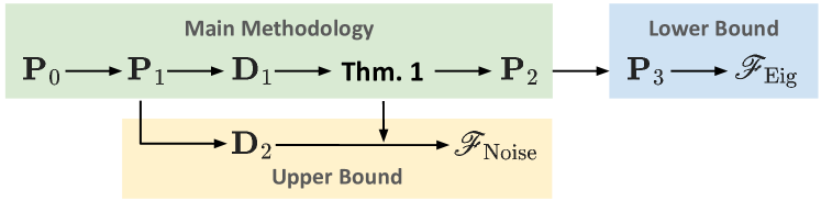
Figure 1: An illustration of the main methodology and suboptimal solutions.

V Main Methodology

To begin with, we use the principle of dynamic programming to reduce a DRPP problem into solving one-step DRPPs. A discussion on when dynamic programming fails is provided. Then, we canonicalize the ambiguity set of SDS into consistent constraints, such that the problem is transformed into an infinite dimensional conic linear program. Next, we take the dual form of inner minimization with a strong duality guarantee. Based on the dual analysis, we develop a necessary optimality condition to handle the essential hardness of functional optimization. Exploiting this optimality condition, we equivalently transform the one-step DRPP in function spaces into a convex-nonconcave minimax problem in Euclidean spaces. Finally, we provide a discussion on the computation complexity.

V-A Dynamic Programming and One-step DRPP

Given a state-control pair $z_{k}$ at time step $k\in\{0,\ldots,T-1\}$, we denote the optimal worst-case value function as

$$V^{*}_{k}(z_{k})=\sup_{\mathscr{F}_{k:T-1}}\inf_{\Phi_{k:T-1}}V^{\mathscr{F}}_{k}(z_{k}).$$ (6)

Leveraging the principle of dynamic programming, one can derive the following recursive equations for $V^{*}_{k}$,

$$V^{*}_{k}(z_{k})=\sup_{\mathscr{F}_{k:T-1}}\inf_{\Phi_{k:T-1}}\mathbb{E}\left[\mathcal{L}(\mathscr{F}_{k}(z_{k}),\boldsymbol{x}_{k+1})\right.$$ (7)

$$\qquad\qquad\left.+\sum_{t=k+1}^{T-1}\mathcal{L}\left(\mathscr{F}_{t}(\boldsymbol{z}_{t}),\boldsymbol{x}_{t+1}\right)\biggm{|}\boldsymbol{z}_{k}=z_{k}\right]$$

$$\overset{(i)}{=} \sup_{\mathscr{F}_{k:T-1}}\left\{\inf_{\Phi_{k}}\mathbb{E}\mathcal{L}(\mathscr{F}_{k}(z_{k}),\boldsymbol{x}_{k+1})\right.$$

$$\qquad\qquad\left.+\inf_{\Phi_{k+1:T-1}}\mathbb{E}\left[V^{\mathscr{F}}_{k+1}(\boldsymbol{z}_{k+1})\biggm{|}\boldsymbol{z}_{k}=z_{k}\right]\right\}$$

$$= \sup_{\mathscr{F}_{k}}\inf_{\Phi_{k}\in\mathcal{I}_{k}}\mathbb{E}\mathcal{L}(\mathscr{F}_{k}(z_{k}),\boldsymbol{x}_{k+1})$$

$$\qquad\qquad+\mathbb{E}\left[V^{*}_{k+1}(\boldsymbol{z}_{k+1})\biggm{|}\boldsymbol{z}_{k}=z_{k}\right].$$

Remark 2.

The equality $(i)$ may not hold when the system dynamics is assumed to be strictly time-invariant, because the worst-case SDSs that minimize the first term $\mathbb{E}\mathcal{L}(\mathscr{F}_{k}(z_{k}),\boldsymbol{x}_{k+1})$ are not guaranteed to minimize the second term $\mathbb{E}\left[V^{\mathscr{F}}_{k+1}(\boldsymbol{z}_{k+1})\biggm{|}\boldsymbol{z}_{k}=z_{k}\right]$. In this case, the problem of DRPP for SDS will not possess an optimal substructure [39], thus the principle of dynamic programming fails to apply.

Thanks to the principle of dynamic programming, one has that the optimal predictor at time step $k$ is

$$\mathscr{F}_{k}^{*}(z)=\arg\sup_{\mathscr{F}_{k}}\inf_{\Phi_{k}}\mathbb{E}\mathcal{L}(\mathscr{F}_{k}(z),\boldsymbol{x}_{k+1}),\forall z\in\mathbb{R}^{d_{x}+d_{u}}.$$

Conditioned on the previous state-control pair $z_{k}$, optimizing over the probabilistic predictor $\mathscr{F}_{k}$ is equivalent to optimizing over the predictive pdf. Therefore, conditioned on $z_{k}$ at time step $k\in\{0,\ldots,T-1\}$, we call the maximin optimization over the predictive pdf space $\mathcal{P}(\mathbb{R}^{d_{x}})$ and the ambiguity set $\mathcal{I}_{k}$ as a one-step DRPP:

$$(\mathbf{P}_{1}):\quad\sup_{\hat{p}_{k}\in\mathcal{P}(\mathbb{R}^{d_{x}})}\inf_{\Phi_{k}\in\mathcal{I}_{k}}\mathbb{E}\;\mathcal{L}(\hat{p}_{k},\boldsymbol{x}_{k+1}),$$

where $\hat{p}_{k}(\cdot):=\mathscr{F}_{k}(z_{k})=\hat{p}_{\boldsymbol{x}_{k+1}\mid\boldsymbol{z}_{k}}(\cdot\mid z_{k})$ is an abbreviation for the predictive pdf of $\boldsymbol{x}_{k+1}$ conditioned on $z_{k}$. In the rest of this paper, we focus on solving the one-step DRPP $\mathbf{P}_{1}$.

V-B Ambiguity Set Constraints Canonicalization

Towards solving the one-step DRPP $\mathbf{P}_{1}$, the very first step is to canonicalize the conic moment-based ambiguity set $\mathcal{I}_{k}$ such that all the optimization variables appeared in the objective and constraints are consistent.

First, to canonicalize the first ambiguity constraint on $f_{k}$, given a state-control pair $z_{k}$ at time step $k$, we define the real one-step state evolution as $\nu_{k}=f_{k}(z_{k})$, and the nominal one-step state evolution as $\bar{\nu}_{k}=\bar{f}_{k}(z_{k})$. Then, this ambiguity constraint of $f_{k}$ is equivalent to describing the distance between $\nu_{k}$ and $\bar{\nu}_{k}$, i.e.,

$$\|\nu_{k}-\bar{\nu}_{k}\|_{2}^{2}= \|f_{k}(z_{k})-\bar{f}_{k}(z_{k})\|_{2}^{2}\leq\gamma_{0,k}(z_{k}).$$

Second, to canonicalize the remaining ambiguity constraints on $p_{\boldsymbol{w}_{k}\mid\boldsymbol{z}_{k}(\cdot\mid z_{k})}$, we need to keep them consistent with the pdf $p_{\boldsymbol{x}_{k+1}\mid\boldsymbol{z}_{k}}(\cdot\mid z_{k})$ in the optimization objective. For ease of notation, since the one-step DRPP problem is always conditioned on a given state-control pair $z_{k}$, we abbreviate the notations by denoting $p_{\boldsymbol{\xi}_{k}}(\cdot)=p_{\boldsymbol{x}_{k+1}\mid\boldsymbol{z}_{k}}(\cdot\mid z_{k})$ and $p_{\boldsymbol{w}_{k}}(\cdot)=p_{\boldsymbol{w}_{k}\mid\boldsymbol{z}_{k}}(\cdot\mid z_{k})$ without raising confusion. It follows that $p_{\boldsymbol{\xi}_{k}}(\xi)=p_{\boldsymbol{w}_{k}}(\xi-\nu_{k})$, and we shall align one with another. Here we align $p_{\boldsymbol{w}_{k}}$ with $p_{\boldsymbol{\xi}_{k}}$ and then optimize over $p_{\boldsymbol{\xi}_{k}}$. Finally, the inner minimization of the one-step DRPP is canonicalized as an infinite dimensional conic linear program:

$$\inf_{\nu_{k},\mu_{k},p_{\boldsymbol{\xi}_{k}}}\;\mathbb{E}_{\xi\sim p_{\boldsymbol{\xi}_{k}}}\log[\hat{p}_{k}(\xi)]$$ (8)

$$\text{s.t.}\left\{\begin{aligned} &\mathbb{E}_{\xi\sim p_{\boldsymbol{\xi}_{k}}}[1]=1,\mathbb{E}_{\xi\sim p_{\boldsymbol{\xi}_{k}}}[\xi]=\mu_{k}+\nu_{k}\\ &\gamma_{3,k}\bar{\Sigma}_{k}\!\preceq\!\mathbb{E}_{\xi\sim p_{\boldsymbol{\xi}_{k}}}\!\left[\left(\xi\!-\!\nu_{k}\!-\!\bar{\mu}_{k}\right)\left(\xi\!-\!\nu_{k}\!-\!\bar{\mu}_{k}\right)^{\mathrm{T}}\right]\!\preceq\!\gamma_{2,k}\bar{\Sigma}_{k}\\ &\left[\begin{array}[]{cc}\bar{\Sigma}_{k}&\left(\mu_{k}-\bar{\mu}_{k}\right)\\ \left(\mu_{k}-\bar{\mu}_{k}\right)^{\top}&\gamma_{1,k}\end{array}\right]\succeq 0\\ &\left[\begin{array}[]{cc}I&\left(\nu_{k}-\bar{\nu}_{k}\right)\\ \left(\nu_{k}-\bar{\nu}_{k}\right)^{\top}&\gamma_{0,k}(z_{k})\end{array}\right]\succeq 0\\ &p_{\boldsymbol{\xi}_{k}}(\xi)\geq 0\quad\forall\xi\in\mathbb{R}^{d_{x}}.\end{aligned}\right.$$

Remark 3.

In fact, the alignment order shall not be reversed, a discussion on why aligning $p_{\boldsymbol{\xi}_{k}}$ with $p_{\boldsymbol{w}_{k}}$ and then optimizing over $p_{\boldsymbol{w}_{k}}$ leads to a dead end is provided in Appendix A.

V-C Dual Analysis

Directly solving the worst-case pdf in the function space $\mathcal{P}(\mathbb{R}^{d_{x}})$ is difficult. As a first step towards dealing with this challenge, we leverage the dual analysis for problem $\mathbf{P}_{1}$. If a strong duality holds, one can optimize the Lagrange multipliers in the dual form. For the inner optimization (8), a classical conclusion is that $\bar{\Sigma}_{k}\succ 0$ is a sufficient condition for strong duality to hold [10, p. 5]. Let $r\in\mathbb{R},q\in\mathbb{R}^{d_{x}},Q_{i}\in S_{+}^{d_{x}},\kappa_{i}=\{P_{i}\in S_{+}^{d_{x}},p_{i}\in\mathbb{R}^{d_{x}},s_{i}\in\mathbb{R}\}$ for $i=1,2$ be the Lagrange multipliers, the dual form of (8) is

$$(\mathbf{D}_{1}): \sup_{\hat{p}_{k},r,q,Q_{1},Q_{2},\kappa_{1},\kappa_{2}}G(r,q,Q_{1},Q_{2},\kappa_{1},\kappa_{2})$$

$$\text{s.t.}\left\{\begin{aligned} &\mathbb{E}_{\xi\sim\hat{p}_{k}}1=1,\hat{p}_{k}(\xi)\geq 0\quad\forall\xi\in\mathbb{R}^{d_{x}}\\ &\xi^{\top}\!(Q_{1}\!-\!Q_{2})\xi\!+\!\xi^{\top}q\!+\!r\!+\!\log\hat{p}_{k}(\xi)\geq 0\;\forall\xi\in\mathbb{R}^{d_{x}}\\ &q+2p_{1}+2(Q_{1}-Q_{2})(\nu_{k}+\bar{\mu}_{k})=0\\ &\left[\begin{array}[]{cc}P_{1}&p_{1}\\ p_{1}^{\top}&s_{1}\end{array}\right]\succeq 0,\left[\begin{array}[]{cc}P_{2}&p_{2}\\ p_{2}^{\top}&s_{2}\end{array}\right]\succeq 0.\end{aligned}\right.$$

where $G(r,q,Q_{1},Q_{2},\kappa_{1},\kappa_{2})\!=\!-r\!+\!\bar{\mu}_{k}^{\top}\!(Q_{1}\!-\!Q_{2})\bar{\mu}_{k}-(\gamma_{2,k}Q_{1}-\gamma_{3,k}Q_{2}+P_{1})\cdot\bar{\Sigma}_{k}-P_{2}\cdot I+2p_{1}^{\top}\bar{\mu}_{k}-s_{1}\gamma_{1,k}+2p_{2}^{\top}\bar{\nu}_{k}-s_{2}\gamma_{0,k}\|z_{k}\|^{2}_{2}-(q+2p_{2})^{\top}\nu_{k}-\nu_{k}^{\top}(Q_{1}-Q_{2})\nu_{k}$. Please see Appendix B for a detailed derivation.

Unfortunately, we have to deal with an infinite number of constraints indexed by $w\in\mathbb{R}^{d_{x}}$ in problem $\mathbf{D}_{1}$. Although the dual problem cannot lead to a direct solution, it helps to develop an optimality condition for the probabilistic predictors in the following theorem.

Theorem 1 (Optimality condition).

A necessary optimality condition for the one-step DRPP $\mathbf{P}_{1}$ is that $\hat{p}_{k}$ is subject to a Gaussian distribution almost everywhere, i.e., $\exists\;\hat{\mu}_{k}\in\mathbb{R}^{d_{x}}$ and $\hat{\Sigma}_{k}\in S^{d_{x}}_{+}$ such that

$$\hat{p}_{k}\overset{\text{a.s.}}{\sim}\mathcal{N}\left(\hat{\mu}_{k},\hat{\Sigma}_{k}\right).$$ (9)

Proof.

Please see Appendix C. ∎

Theorem 1 reduces the optimization complexity from the original function space $\mathcal{P}(\mathbb{R}^{d_{x}})$ to the Gaussian distribution family, more specifically, the parameter spaces of mean and covariance. Therefore, $\mathbf{D}_{1}$ can be transformed into a finite-dimensional optimization problem as follows

$$\max_{\hat{\mu}_{k},\hat{\Sigma}_{k},Q_{1},Q_{2},\kappa_{1},\kappa_{2}}-\frac{1}{2}d_{x}\log(2\pi)\!+\!\frac{1}{2}\log\operatorname{det}(\hat{\Sigma}_{k}^{-1})$$ (10)

$$-(\gamma_{2,k}Q_{1}\!-\!\gamma_{3,k}Q_{2})\!\cdot\!\bar{\Sigma}_{k}-P_{1}\!\cdot\!\bar{\Sigma}_{k}-P_{2}\!\cdot\!I-s_{1}\gamma_{1,k}$$

$$-s_{2}\gamma_{0,k}\|z_{k}\|^{2}_{2}+2p_{1}^{\top}\!\hat{\Sigma}_{k}(2p_{2}\!-\!p_{1})-2p_{2}^{\top}(\hat{\mu}_{k}\!-\!\bar{\mu}_{k}\!-\!\bar{\nu}_{k})$$

$$\text{s.t.}\left\{\begin{aligned} &Q_{1}\succeq 0,Q_{2}\succeq 0,Q_{1}-Q_{2}=\frac{1}{2}\hat{\Sigma}_{k}^{-1},\hat{\Sigma}_{k}\succ 0\\ &\left[\begin{array}[]{cc}P_{1}&p_{1}\\ p_{1}^{\top}&s_{1}\end{array}\right]\succeq 0,\left[\begin{array}[]{cc}P_{2}&p_{2}\\ p_{2}^{\top}&s_{2}\end{array}\right]\succeq 0.\end{aligned}\right.$$

Please see Appendix D for a detailed derivation. However, this problem is now a nonconvex semidefinite optimization with respect to $\hat{\Sigma}_{k}$, solving a globally optimal solution is NP-hard in general. An alternative is to use numerical iterative algorithms to seek a locally optimal solution of (10). Nevertheless, the local optimality of the dual problem cannot guarantee the worst-case performance of $\mathbf{P}_{1}$. To deal with this hardness, we avoid directly solving the dual problem by applying the optimality condition in Theorem 1 to $\mathbf{P}_{1}$.

V-D Primal Analysis Under Gaussian Parameterization

Substituting the parameterized $\hat{p}_{k}$ into the primal one-step DRPP $\mathbf{P}_{1}$, we have the objective being as

$$\mathbb{E}_{\xi\sim p_{\boldsymbol{\xi}_{k}}}\!\!-\!\frac{1}{2}[d_{x}\log(2\pi)\!+\!\log\operatorname{det}(\hat{\Sigma}_{k})\!+\!(\xi\!-\!\hat{\mu}_{k})\hat{\Sigma}_{k}^{-1}(\xi\!-\!\hat{\mu}_{k})\!^{\top}].$$

Next, notice that $\mathbb{E}_{\xi\sim p_{\boldsymbol{\xi}_{k}}}[\xi]=\mu_{k}+\nu_{k}$ and $\mathbb{E}_{\xi\sim p_{\boldsymbol{\xi}_{k}}}(\xi-\nu_{k}\!-\mu_{k})(\xi-\nu_{k}-\mu_{k})^{\top}=\Sigma_{k}$, one has $\mathbb{E}_{\xi\sim p_{\boldsymbol{\xi}_{k}}}(\xi-\hat{\mu}_{k})\hat{\Sigma}_{k}^{-1}(\xi-\hat{\mu}_{k})^{\top}$ equals to $[\Sigma_{k}+(\mu_{k}+\nu_{k}-\hat{\mu}_{k})(\mu_{k}+\nu_{k}-\hat{\mu}_{k})^{\top}]\cdot\hat{\Sigma}_{k}^{-1}$. The functional minimax $\mathbf{P}_{1}$ is then equivalent to a minimax optimization in Euclidean spaces as follows

$$(\mathbf{P}_{2}): \min_{\hat{\Sigma}_{k},\hat{\mu}_{k}}\max_{\Sigma_{k},\mu_{k},\nu_{k}}-\log\operatorname{det}(\hat{\Sigma}_{k}^{-1})$$

$$\qquad+\left[\Sigma_{k}\!+\!(\mu_{k}\!+\!\nu_{k}\!-\!\hat{\mu}_{k})(\mu_{k}\!+\!\nu_{k}\!-\!\hat{\mu}_{k})^{\top}\right]\!\cdot\!\hat{\Sigma}_{k}^{-1}$$

$$\text{s.t.}\left\{\begin{aligned} &\|\nu_{k}-\bar{\nu}_{k}\|_{2}^{2}\leq\gamma_{0,k}(z_{k}),\|\mu_{k}-\bar{\mu}_{k}\|_{\bar{\Sigma}_{k}^{-1}}^{2}\leq\gamma_{1,k}\\ &\gamma_{3,k}\bar{\Sigma}_{k}\preceq\Sigma_{k}+(\mu_{k}-\bar{\mu}_{k})(\mu_{k}-\bar{\mu}_{k})^{\top}\preceq\gamma_{2,k}\bar{\Sigma}_{k}.\end{aligned}\right.$$

Lemma 1.

Given any $\mu_{k}$, the one-step DRPP $\mathbf{P}_{2}$ has explicit solutions for $\Sigma_{k}$ and $\hat{\mu}_{k}$ as
i) $\Sigma_{k}^{*}=\gamma_{2,k}\bar{\Sigma}_{k}-(\mu_{k}-\bar{\mu}_{k})(\mu_{k}-\bar{\mu}_{k})^{\top}$.
ii) $\hat{\mu}^{*}_{k}=\bar{\mu}_{k}+\bar{\nu}_{k}$.

Proof.

Please see Appendix E. ∎

Substituting the expressions of $\Sigma_{k}^{*}$ and $\hat{\mu}_{k}^{*}$ into $\mathbf{P}_{2}$, it is equivalent to a convex-nonconcave minimax optimization:

$$\min_{\hat{\Sigma}_{k}\succ 0}\max_{a,b}\;-\log\operatorname{det}(\hat{\Sigma}_{k}^{-1})+\gamma_{2,k}\bar{\Sigma}_{k}\cdot\hat{\Sigma}_{k}^{-1}$$ (11)

$$\qquad\qquad+\|a+b\|_{\hat{\Sigma}_{k}^{-1}}^{2}-\|a\|_{\hat{\Sigma}_{k}^{-1}}^{2}$$

$$\text{s.t.}\;\|a\|_{\bar{\Sigma}_{k}^{-1}}^{2}\leq\gamma_{1,k},\|b\|_{2}^{2}\leq\gamma_{0,k}(z_{k}),$$

where $a=\mu_{k}-\bar{\mu}_{k},b=\nu_{k}-\bar{\nu}_{k}$. Notice that the inner maximization is an indefinite quadratic constrained quadratic programming (QCQP) problem, which is still short of efficient algorithms to solve this kind of minimax optimization.

Given any $\hat{\Sigma}_{k}\succ 0$ and $b\neq 0$, one can first solve $a$ by concerning the following quadratic constrained linear programming (QCLP) problem:

$$\max_{a}\|a+b\|_{\hat{\Sigma}_{k}^{-1}}^{2}-\|a\|_{\hat{\Sigma}_{k}^{-1}}^{2}\text{ s.t. }\|a\|_{\bar{\Sigma}_{k}^{-1}}^{2}\leq\gamma_{1,k}.$$ (12)

Lemma 2.

The solution of the QCLP problem (12) is

$$a^{*}=\frac{\sqrt{\gamma_{1,k}}\bar{\Sigma}_{k}\hat{\Sigma}_{k}^{-1}b}{\|\bar{\Sigma}_{k}\hat{\Sigma}_{k}^{-1}b\|_{\bar{\Sigma}_{k}^{-1}}}.$$

Proof.

Using the KKT condition, there are

$$\left\{\begin{aligned} &\partial_{a}\left[\|a+b\|_{\hat{\Sigma}_{k}^{-1}}^{2}-\|a\|_{\hat{\Sigma}_{k}^{-1}}^{2}-s_{1}(\|a\|_{\bar{\Sigma}_{k}^{-1}}^{2}-\gamma_{1})\right]=0\\ &s_{1}(\|a\|_{\bar{\Sigma}_{k}^{-1}}^{2}-\gamma_{1})=0,s_{1}\geq 0\\ \end{aligned}\right.$$

The first condition reveals that $s_{1}\neq 0$ and $a=s_{1}^{-1}\bar{\Sigma}_{k}\hat{\Sigma}_{k}^{-1}b$, thus the second condition leads to $\|a\|_{\bar{\Sigma}_{k}^{-1}}^{2}=\gamma_{1,k}$. Then,

$$s_{1}=\frac{\|\bar{\Sigma}_{k}\hat{\Sigma}_{k}^{-1}b\|_{\bar{\Sigma}_{k}^{-1}}}{\|a\|_{\bar{\Sigma}_{k}^{-1}}}=\frac{\|\bar{\Sigma}_{k}\hat{\Sigma}_{k}^{-1}b\|_{\bar{\Sigma}_{k}^{-1}}}{\sqrt{\gamma_{1,k}}},$$

and the proof is completed. ∎

Substituting the optimal $a^{*}$ into the problem, the inner optimization of (11) can be further reformulated as a convex maximization problem:

$$\max_{b}\;\alpha\|b\|_{A}+\|b\|_{B}^{2}\text{ s.t. }\|b\|_{2}^{2}\leq\gamma_{0,k}(z_{k}),$$ (13)

where $A=\hat{\Sigma}_{k}^{-1}\bar{\Sigma}_{k}\hat{\Sigma}_{k}^{-1}$, $B=\hat{\Sigma}_{k}^{-1}$, and $\alpha=2\sqrt{\gamma_{1,k}}$.

V-E Complexity Analysis

As we have shown, solving the one-step DRPP $\mathbf{P}_{1}$ is equivalent to finding a global minimax point (Stackelberg equilibrium) for a convex-nonconcave minimax problem where the outer minimization is a semidefinite programming and the inner problem is to maximize a non-smooth convex function subject to quadratic constraint. It is known that convex maximization is NP-hard in very simple cases such as quadratic maximization over a hypercube, and even verifying local optimality is NP-hard [40]. Thus finding a global minimax point of a one-step DRPP problem is also NP-hard.

Even worse, finding a local minimax point of a general constrained minimax optimization is of fundamental hardness. Not only the local minimax point may not exist [41], but any gradient-based algorithm needs exponentially many queries in the dimension and $\epsilon^{-1}$ to compute an $\epsilon$-approximate first-order local stationary point [42]. Finally, the local stationary point is not always guaranteed to be a local minimax point [43, 44].

In summary, globally finding a minimax point of a one-step DRPP is computationally intractable, and gradient-based algorithms aiming for local minimax points are limited by both convergence speed and performance guarantee. Therefore, a reasonable goal for the one-step DRPP is to derive upper or lower bounds of the optimal worst-case value function $V_{k}^{*}$ by relaxing the constraints imposed on the predictors or SDSs.

VI Value Function Upper Bound

To get an upper bound of $V_{k}^{*}$, one can either enlarge the feasible region of the outer maximization or shrink the feasible region of the inner minimization. Since the outer feasible region has already contained all pdfs, we shall weaken some constraints of the ambiguity set $\mathcal{I}_{k}$. If the first constraint is substituted by $\nu_{k}=\bar{\nu}_{k}$, one is constrained to a smaller ambiguity subset of $\mathcal{I}_{k}$. If a global minimax point can be solved for the relaxed one-step DRPP, one will get a suboptimal predictor and a performance upper bound.

VI-A Problem Reformulation

If we shrink the ambiguity set of one-step DRPP $\mathbf{P}_{1}$ by assuming that the nominal one-step state evolution $\bar{\nu}_{k}$ is equal with the nominal one-step state evolution $\nu_{k}$, there is $w_{k}=x_{k+1}-\bar{\nu}_{k},$ which means that the value of $w_{k}$ is precisely known after $x_{k+1}$ been observed.

Remark 4.

Now that there is no uncertainty of the state evolution $\nu_{k}$, intuition is that predicting the state’s conditional pdf $p_{\boldsymbol{x}_{k+1}\mid\boldsymbol{z}_{k}}$ is equivalent to predicting the noise’s conditional pdf $p_{\boldsymbol{w}_{k}\mid\boldsymbol{z}_{k}}$. To delineate this intuition in rigor, we construct an auxiliary predictive pdf $\hat{p}_{\boldsymbol{w}_{k}\mid\boldsymbol{z}_{k}}$ as

$$\hat{p}_{\boldsymbol{w}_{k}\mid\boldsymbol{z}_{k}}(w_{k}\mid z_{k}):=\hat{p}_{\boldsymbol{x}_{k+1}\mid\boldsymbol{z}_{k}}(w_{k}+\bar{\nu}_{k}\mid z_{k})=\hat{p}_{k}(x_{k+1}).$$

Then, the objective of the one-step DRPP $\mathbf{P}_{1}$, which is originally an expectation over $\boldsymbol{x}_{k+1}$ conditioned on $z_{k}$, now equals an expectation over $\boldsymbol{w}_{k}$ conditioned on $z_{k}$, i.e.,

$$\mathbb{E}_{x_{k+1}\sim p_{\boldsymbol{x}_{k+1}\mid\boldsymbol{z}_{k}}(\cdot\mid z_{k})}\log\hat{p}_{k}(x_{k+1})$$

$$= \mathbb{E}_{w_{k}\sim p_{\boldsymbol{w}_{k}\mid\boldsymbol{z}_{k}}(\cdot\mid z_{k})}\log\hat{p}_{\boldsymbol{w}_{k}\mid\boldsymbol{z}_{k}}(w_{k}\mid z_{k}).$$

As a result, the outer optimization of $\mathbf{P}_{1}$ that maximizes over $\hat{p}_{k}$ can be recast to maximize over $\hat{p}_{\boldsymbol{w}_{k}\mid\boldsymbol{z}_{k}}(\cdot\mid z_{k})$.

To summarize, the essence of probabilistic prediction subject to no uncertainty of one-step state evolution is to predict the noise’s conditional distribution.

Conditioned on $z_{k}$, we let $\mu_{k}$ be the conditional expectation of $\boldsymbol{w}_{k}$ and abbreviate the conditional pdf $p_{\boldsymbol{w}_{k}\mid\boldsymbol{z}_{k}}(\cdot\mid z_{k})$ as $p_{\boldsymbol{w}_{k}}$. Different from the general condition as discussed in Remark 3 where one should not formulate the inner minimization over $p_{\boldsymbol{w}_{k}}$, now the inner minimization can be structured as a canonical moment problem on $\mu_{k}$ and $p_{\boldsymbol{w}_{k}}$:

$$\inf_{\mu_{k},p_{\boldsymbol{w}_{k}}}\;\mathbb{E}_{w\sim p_{\boldsymbol{w}_{k}}}\log[\hat{p}_{k}(w+\bar{\nu}_{k})]$$ (14)

$$\text{s.t.}\left\{\begin{aligned} &\mathbb{E}_{w\sim p_{\boldsymbol{w}_{k}}}[1]=1,\mathbb{E}_{w\sim p_{\boldsymbol{w}_{k}}}[w]=\mu_{k}\\ &\gamma_{3,k}\bar{\Sigma}_{k}\preceq\mathbb{E}_{w\sim p_{\boldsymbol{w}_{k}}}\!\left[\left(w-\bar{\mu}_{k}\right)\left(w-\bar{\mu}_{k}\right)^{\top}\right]\preceq\gamma_{2,k}\bar{\Sigma}_{k}\\ &\left[\begin{array}[]{cc}\bar{\Sigma}_{k}&\left(\mu-\bar{\mu}_{k}\right)\\ \left(\mu-\bar{\mu}_{k}\right)^{\top}&\gamma_{1,k}\end{array}\right]\succeq 0\\ &p_{\boldsymbol{w}_{k}}(w)\geq 0\quad\forall w\in\mathbb{R}^{d_{x}}.\end{aligned}\right.$$

With the outer maximization imposed on $\hat{p}_{k}$, we can get a reformulated one-step DRPP whose optimal worst-case value function is an upper bound of $V^{*}(z_{k})$.

VI-B Noise-DRPP

Taking the dual form of the inner moment problem and joining it with the outer maximization, we transform the primal maximin problem into the following maximization problem:

$$(\mathbf{D}_{2}): \sup_{\hat{p}_{k},r,q,Q_{1},Q_{2},P,p,s}G(r,q,Q_{1},Q_{2},P,p,s)$$

$$\text{s.t.}\left\{\begin{aligned} &\mathbb{E}_{\xi\sim\hat{p}_{k}}1=1,\hat{p}_{k}(\xi)\geq 0\quad\forall\xi\in\mathbb{R}^{d_{x}}\\ &w^{\top}\!(Q_{1}\!-\!Q_{2})w\!+\!w^{\top}q\!+\!r\!+\!\log\hat{p}_{k}(w\!+\!\bar{\nu}_{k})\!\geq\!0\\ &\qquad\qquad\qquad\qquad\qquad\;\;\forall w\!\in\!\mathbb{R}^{d_{x}}\\ &q+2(Q_{1}-Q_{2})\bar{\mu}_{k}+2p=0\\ &Q_{1}\succeq 0,Q_{2}\succeq 0\\ &\left[\begin{array}[]{cc}P&p\\ p^{\top}&s\end{array}\right]\succeq 0,\end{aligned}\right.$$

where $G(r,q,Q_{1},Q_{2},P,p,s)=-r+\bar{\mu}_{k}^{\top}(Q_{1}-Q_{2})\bar{\mu}_{k}-(\gamma_{2,k}Q_{1}-\gamma_{3,k}Q_{2}+P)\cdot\bar{\Sigma}_{k}+2p^{\top}\bar{\mu}_{k}-s\gamma_{1,k}$. Please see Appendix F for a detailed derivation for the dual problem.

Theorem 2 (Noise-DRPP).

Given $z_{k}=(x_{k},u_{k})$ at time step $k\in\{0,\ldots,T-1\}$, if the probabilistic predictor has no ambiguity of the one-step state evolution, i.e., $\bar{\nu}_{k}=\nu_{k}$, the solution to the one-step DRPP $\mathbf{P}_{1}$ is:
i) The optimal predictive pdf is

$$\hat{p}^{*}_{k}\sim\mathcal{N}\left(\bar{\nu}_{k}+\bar{\mu}_{k},\;\gamma_{2,k}\bar{\Sigma}_{k}\right).$$

ii) The worst-case SDS $\Phi^{*}_{k}$ belongs to the set

$$\left\{\begin{array}[]{c|c}(f_{k},p_{\boldsymbol{w}_{k}})&\begin{aligned} &f_{k}(z_{k})=\bar{f}_{k}(z_{k})\\ &\mathbb{E}_{w\sim p_{\boldsymbol{w}_{k}}}[(w-\bar{\mu}_{k})(w-\bar{\mu}_{k})^{\top}]\!=\!\gamma_{2,k}\bar{\Sigma}_{k}\end{aligned}\end{array}\right\}.$$

iii) The objective value at $(\hat{p}^{*}_{k},\Phi^{*}_{k})$ is

$$-\frac{1}{2}\left[d_{x}\log(2\pi)+d_{x}+\log\operatorname{det}(\gamma_{2,k}\bar{\Sigma}_{k})\right].$$

Proof.

Please see Appendix G. ∎

First, an immediate application of Theorem 2 is to utilize the explicit solution of $\hat{p}^{*}_{k}$ to develop a probabilistic prediction algorithm. Because this predictor solely focuses on the distributional robustness against the ambiguity of system noises, we name it Noise-DRPP. The pseudo-code is in Algorithm 1.

Second, notice that the optimal predictive pdf is unique, but the worst-case SDS is not. It contains any SDS that has a proper one-step state evolution and a noise whose first two moments satisfy an equation.

Finally, which is also our original goal, the objective value at $(\hat{p}^{*}_{k},\Phi^{*}_{k})$ is an upper bound of $V_{k}^{*}(z_{k})$. Since the objective value does not depend on $z_{k}$, we can recursively use the dynamic programming (7) to get an upper bound of $V^{*}$.

Theorem 3 (Upper bound of $V^{*}$).

Given an initial state-control pair $z_{0}=(x_{0},u_{0})$, an upper bound of the optimal worst-case value function $V^{*}(z_{0})$ is

$$V^{*}(z_{0})\leq\sum_{k=0}^{T-1}-\frac{1}{2}\left[d_{x}\log(2\pi)+d_{x}+\log\operatorname{det}(\gamma_{2,k}\bar{\Sigma}_{k})\right].$$

Remark 5.

We highlight that this upper bound can be computed offline because it only depends on the ambiguity sets $\mathcal{I}_{0:T-1}$. It can be used to verify whether the current ambiguity set is too conservative by comparing it with the real-time performance of a Noise-DRPP predictor in practice: if the scores always exceed this upper bound, one can suspect that the ambiguity set is too large.

Algorithm 1 Noise-DRPP $\mathscr{F}_{\text{Noise}}$

1:time horizon $T$, ambiguity sets $\mathcal{I}_{0:T-1}$, control policy $\pi_{0:T-1}$, initial state $x_{0}$.

2:$s_{0}\leftarrow 0$. $\triangleright$ score at time step $0$

3:for $k=0,\ldots,T-1$ do

4:     Predictor updates ambiguity set $\mathcal{I}_{k}$ as (4).

5:     SDS generates control input $u_{k}\sim\pi_{k}(\cdot\mid x_{k})$.

6:     $z_{k}\leftarrow(x_{k},u_{k})$, $\bar{\nu}_{k}\leftarrow\bar{f}_{k}(z_{k})$.

7:     Predictor predicts $\hat{p}_{k}^{*}\sim\mathcal{N}\left(\bar{\nu}_{k}+\bar{\mu}_{k},\;\gamma_{2,k}\bar{\Sigma}_{k}\right)$.

8:     SDS generates the next state $x_{k+1}$.

9:     $s_{k+1}\leftarrow s_{k}+\mathcal{L}(\hat{p}_{k}^{*},x_{k+1})$.

10:end for

11:states $x_{0:T}$, predictions $\hat{p}^{*}_{0:T-1}$, scores $s_{0:T}$.

VII Value function Lower Bound

To get a lower bound of $V^{*}_{k}$, one can either shrink the feasible region of the outer maximization or enlarge the feasible region of the inner minimization. Because enlarging the ambiguity set does not essentially change the structure to alleviate the difficulty of a one-step DRPP $\mathbf{P}_{2}$, we choose to restrict $\hat{p}_{k}$ to a smaller pdf family by forcing the eigenvectors of the predictive covariance $\hat{\Sigma}_{k}$ to be the same as the nominal covariance $\bar{\Sigma}_{k}$. In this section, we elaborate on how the eigenvector restriction contributes to a well-performed algorithm and a lower bound.

VII-A Problem Reformulation

After relaxing the constraints of (11), one can still get a suboptimal prediction performance guarantee in the worst case, which is also a performance lower bound to the original one-step DRPP. Nevertheless, the choice of relaxation methods is delicate, which can greatly affect both the optimality gap and the computation efficiency.

Suppose the spectral decomposition for $\bar{\Sigma}_{k}$ is $Q_{k}\Lambda_{k}Q_{k}^{\top}$, where $Q_{k}=[\mathbf{v}_{1,k},\ldots,\mathbf{v}_{d_{x},k}]$ is an orthogonal matrix whose columns are eigenvectors of $\bar{\Sigma}_{k}$ and $\Lambda_{k}=\operatorname{diag}\{\lambda_{1,k},\ldots,\lambda_{d_{x},k}\}$. Similarly, we let the spectral decomposition for $\hat{\Sigma}_{k}$ be $\hat{Q}_{k}\hat{\Lambda}_{k}\hat{Q}_{k}^{\top}$, where $\hat{Q}_{k}$ is an orthogonal matrix whose columns are eigenvectors of $\hat{\Sigma}_{k}$ and $\hat{\Lambda}_{k}=\operatorname{diag}\{\hat{\lambda}_{1,k},\ldots,\hat{\lambda}_{d_{x},k}\}$. Then, the eigenvector restriction for (11) is to impose the following constraint to the predictor:

$$\hat{Q}_{k}=Q_{k}.$$ (15)

To explain why we chose the eigenvector restriction, some supporting lemmas need to be derived.

Lemma 3.

The optimal $b^{*}$ to problem (13) is an eigenvector of $\frac{\alpha}{\|b^{*}\|_{A}}A+2B$ with its $\ell^{2}$-norm being $\sqrt{\gamma_{0,k}(z_{k})}$.

Proof.

There are necessary optimality conditions for (13):

$$\left\{\begin{aligned} &\left(\frac{\alpha}{\|b\|_{A}}A+2B-2sI\right)b=0\\ &\|b\|_{2}^{2}=\gamma_{0,k}(z_{k}),\end{aligned}\right.$$

where the first one comes from the KKT condition and the second one holds because the objective increases monotonously with $\|b\|_{2}$. It follows that the optimal $b$ should be an eigenvector of $\frac{\alpha}{\|b\|_{A}}A+2B$ with its $\ell^{2}$-norm being $\sqrt{\gamma_{0,k}(z_{k})}$. ∎

If the eigenvectors of $\frac{\alpha}{\|b^{*}\|_{A}}A+2B$ have explicit expressions, one may have explicit expressions for $a^{*},b^{*}$. Then, substituting these expressions to (11) can transform the original minimax optimization problem into a semidefinite-constrained maximization, where tractable optimization solvers may be available. However, it is always difficult to explicitly derive the eigenvectors when $\hat{Q}_{k}$ does not identify with $Q_{k}$.

Lemma 4.

When $\hat{Q}_{k}=Q_{k}$ is supplemented to the constraints of (13), the solution is

$$b^{*}=\sqrt{\gamma_{0,k}(z_{k})}\mathbf{v}_{j_{k},k},$$

where $j_{k}=\arg\max\limits_{i}(2\sqrt{\gamma_{0,k}(z_{k})\gamma_{1,k}\lambda_{i,k}}+\gamma_{0,k}(z_{k}))\hat{\lambda}_{i,k}^{-1}$.

Proof.

When $\hat{Q}_{k}=Q_{k}$ is satisfied, there is

$$\frac{\alpha}{\|b\|_{A}}A+2B=Q_{k}\left[\frac{\alpha}{\|b\|_{A}}\hat{\Lambda}_{k}^{-2}\Lambda_{k}+\hat{\Lambda}_{k}^{-1}\right]Q_{k}^{\top},$$

whose eigenvectors are the columns of $Q_{k}$. Lemma 3 indicates that the optimal $b$ can be expressed as $\sqrt{\gamma_{0,k}(z_{k})}\mathbf{v}_{i}$ for certain $i\in\{1,\ldots,d_{x}\}$, then we have the objective of (13) is $(2\sqrt{\gamma_{0,k}(z_{k})\gamma_{1,k}\lambda_{i,k}}+\gamma_{0,k}(z_{k}))\hat{\lambda}_{i,k}^{-1}$. Since $j_{k}=\arg\max_{i}(2\sqrt{\gamma_{0,k}(z_{k})\gamma_{1,k}\lambda_{i,k}}+\gamma_{0,k}(z_{k}))\hat{\lambda}_{i,k}^{-1}$, problem (13) is solved as $b^{*}=\sqrt{\gamma_{0,k}(z_{k})}\mathbf{v}_{j_{k}}$. ∎

Utilizing the expression of $b^{*}$ in Lemma 4, the minimax optimization $\eqref{eq:qcqp}$ under eigenvector restriction (15) can be transformed into

$$(\mathbf{P}_{3}): \min_{\hat{\Lambda}_{k}\succeq 0,j_{k}}\sum_{i=1}^{d_{x}}\left[-\log(\hat{\lambda}_{i,k}^{-1})+\gamma_{2,k}\lambda_{i,k}\hat{\lambda}_{i,k}^{-1}\right]+$$

$$\qquad\left(2\sqrt{\gamma_{0,k}(z_{k})\gamma_{1,k}\lambda_{j_{k},k}}+\gamma_{0,k}(z_{k})\right)\hat{\lambda}_{j_{k},k}^{-1}$$

$$\text{s.t. }\hat{\lambda}_{j_{k},k}\leq\frac{2\sqrt{\gamma_{0,k}(z_{k})\gamma_{1,k}\lambda_{j_{k},k}}\!+\!\gamma_{0,k}(z_{k})}{2\sqrt{\gamma_{0,k}(z_{k})\gamma_{1,k}\lambda_{i,k}}\!+\!\gamma_{0,k}(z_{k})}\hat{\lambda}_{i,k}$$

$$\qquad\qquad\qquad\qquad\qquad\qquad\qquad\forall i\in\{1,\ldots,d_{x}\}.$$

VII-B Eig-DRPP

Notice that optimization $\mathbf{P}_{3}$ is convex for any fixed $j_{k}$. Therefore, $\mathbf{P}_{3}$ can be solved by taking the minimum of $d_{x}$ different convex optimization problems, which is numerically efficient. Let $\left(\hat{\Lambda}_{k}^{*}=\operatorname{diag}\{\hat{\lambda}_{1,k}^{*},\ldots,\hat{\lambda}_{d_{x},k}^{*}\},j_{k}^{*}\right)$ be the solution of $\mathbf{P}_{3}$, we summarize the solution of a one-step DRPP under eigenvector restriction as follows.

Theorem 4 (Eig-DRPP).

Given $z_{k}=(x_{k},u_{k})$ at time step $k\in\{0,\ldots,T-1\}$, if the probabilistic predictor is constrained by the eigenvector restriction (15), the solution to the one-step DRPP $\mathbf{P}_{1}$ is:
i) The optimal predictive pdf $\hat{p}^{*}_{k}$ is

$$\hat{p}_{k}^{*}\sim\mathcal{N}\left(\bar{\nu}_{k}+\bar{\mu}_{k},\;Q_{k}\hat{\Lambda}_{k}^{*}Q_{k}^{\top}\right).$$

ii) The worst-case SDS $\Phi^{*}_{k}$ belongs to the set

$$\left\{\!\begin{array}[]{c|c}(f_{k},p_{\boldsymbol{w}_{k}})&\begin{aligned} &f_{k}(z_{k})=\sqrt{\gamma_{0,k}(z_{k})}\mathbf{v}_{j_{k}^{*}\!,k}+\bar{\nu}_{k}\\ &\mathbb{E}[\boldsymbol{w}_{k}]=\bar{\mu}_{k}+\sqrt{\gamma_{1,k}\lambda_{j_{k}^{*}\!,k}}\mathbf{v}_{j_{k}^{*}\!,k}\\ &\operatorname{Cov}[\boldsymbol{w}_{k}]=\gamma_{2,k}\bar{\Sigma}_{k}-\gamma_{1,k}\lambda_{j_{k}^{*}\!,k}\mathbf{v}_{j^{*}\!,k}\mathbf{v}_{j_{k}^{*}\!,k}^{\top}\end{aligned}\end{array}\right\}.$$

iii) The objective value at $(\hat{p}^{*}_{k},\Phi^{*}_{k})$ is

$$-\frac{1}{2}\left\{d_{x}\log(2\pi)+\sum_{i=1}^{d_{x}}\left[\log(\hat{\lambda}_{i,k}^{*})+\gamma_{2,k}\frac{\lambda_{i,k}}{\hat{\lambda}_{i,k}^{*}}\right]\right.$$

$$\left.\qquad+\frac{2\sqrt{\gamma_{0,k}(z_{k})\gamma_{1,k}\lambda_{j_{k}^{*}\!,k}}+\gamma_{0,k}(z_{k})}{\hat{\lambda}_{j_{k}^{*}\!,k}^{*}}\right\}.$$

Proof.

The proof is completed by combining the results in Lemma 1, Lemma 2, and the solutions of $\mathbf{P}_{3}$. ∎

First, an immediate application of Theorem 4 is to utilize the explicit solution of $\hat{p}^{*}_{k}$ to develop a probabilistic prediction algorithm, named Eig-DRPP. The pseudo-code is presented in Algorithm 2. Second, although the optimal predictive pdf is unique, the worst-case SDS is not. Compared to Theorem 2, there are relatively more restrictions on the set of worst-case SDSs. Third, when $\gamma_{0,k}=0$, i.e., the predictor has no ambiguity of $f_{k}$, the solution of $\mathbf{P}_{3}$ is $\hat{\lambda}_{i,k}^{*}=\gamma_{2,k}\lambda_{i,k}$ and $j_{k}^{*}$ can be any feasible index. In this case, both the optimal predictive pdf and objective value in Theorem (4) coincide with those in Theorem (2). However, the sets of worst-case SDSs are not the same, due to the extra constraint for the expectation in Theorem (4).

Finally, the objective value at $(\hat{p}^{*}_{k},\Phi^{*}_{k})$ is a lower bound of $V_{k}^{*}(z_{k})$. Since the objective value depends on $z_{k}$ through $\gamma_{0,k}(z_{k})$, one cannot directly use the dynamic programming (7) recursively to get a lower bound of $V^{*}$.

Theorem 5 (Lower bound of $V^{*}$ and optimality gap of $\mathscr{F}_{\text{Eig}}$).

Given an initial state-control pair $z_{0}=(x_{0},u_{0})$ and an upper bound of $\gamma_{0,k}$ such that $\gamma_{0,k}(z)\leq\Gamma_{0,k}\in\mathbb{R}_{+},\forall z\in\mathbb{R}^{d_{x}+d_{u}}$ for each $k\in\{0,\cdots,T-1\}$, there is
i) A lower bound of the optimal worst-case function is

$$V^{*}(z_{0})\geq \sum_{k=0}^{T-1}-\frac{1}{2}\left\{d_{x}\log(2\pi)\!+\!\sum_{i=1}^{d_{x}}\left[\log(\hat{\lambda}_{i,k}^{*})\!+\!\gamma_{2,k}\frac{\lambda_{i,k}}{\hat{\lambda}_{i,k}^{*}}\right]\right.$$

$$\left.\qquad+\frac{2\sqrt{\Gamma_{0,k}\gamma_{1,k}\lambda_{j_{k}^{*}\!,k}}+\Gamma_{0,k}}{\hat{\lambda}_{j_{k}^{*}\!,k}^{*}}\right\},$$

where $\hat{\lambda}_{1,k}^{*},\ldots,\hat{\lambda}_{d_{x},k}^{*},j_{k}^{*}$ is the solution to $\mathbf{P}_{3}$ with all $\gamma_{0,k}(z_{k})$ being replaced by $\Gamma_{0,k}$.
ii) The optimality gap between Eig-DRPP $\mathscr{F}_{\text{Eig}}$ and the global optimal predictor is upper bounded as follows,

$$V^{*}(z_{0})-V^{\mathscr{F}_{\text{Eig}}}(z_{0})\leq\sum_{k=0}^{T-1}-\frac{1}{2}\bigg{\{}\underbrace{d_{x}+\log\operatorname{det}(\gamma_{2,k}\bar{\Sigma}_{k})}_{\leavevmode\hbox to9.4pt{\vbox to9.4pt{\text{[drawing]}}}}$$ (16)

$$\underbrace{-\sum_{i=1}^{d_{x}}\left[\log(\hat{\lambda}_{i,k}^{*})\!+\!\gamma_{2,k}\frac{\lambda_{i,k}}{\hat{\lambda}_{i,k}^{*}}\right]-\frac{2\sqrt{\Gamma_{0,k}\gamma_{1,k}\lambda_{j_{k}^{*}\!,k}}+\Gamma_{0,k}}{\hat{\lambda}_{j_{k}^{*}\!,k}^{*}}}_{\leavevmode\hbox to9.4pt{\vbox to9.4pt{\text{[drawing]}}}}\bigg{\}}.$$

Proof.

i) Notice that as $\gamma_{0,k}(z_{k})$ increases, the ambiguity set enlarges, thus the optimal value of one-step DRPP under eigenvector constraint should monotonously decrease. Since the upper bound of $\gamma_{0,k}(z_{k})$, i.e., $\Gamma_{0,k}$, is independent of $z_{k}$, one can still use (7) to derive a lower bound.

ii) Subtracting this lower bound from the upper bound in Theorem 3, one immediately gets an upper bound of the optimality gap for Eig-DRPP. As illustrated in (16), comes from the upper bound, which is determined by $\gamma_{2,k}$ and the determinant of $\bar{\Sigma}_{k}$. While comes from the lower bound, which is jointly determined by $\Gamma_{0,k},\gamma_{1,k},\gamma_{2,k}$ and the eigenvalues of $\bar{\Sigma}_{k}$ by solving $\mathbf{P}_{3}$. ∎

Remark 6.

Similar to the upper bound, this lower bound can also be computed offline because it only depends on the ambiguity sets $\mathcal{I}_{0:T-1}$. It can be used to verify whether the current ambiguity set is too optimistic by comparing it with the real-time performance of an Eig-DRPP predictor in practice: if the scores always stay lower than this lower bound, one can suspect that the ambiguity set is too small.

Algorithm 2 Eig-DRPP $\mathscr{F}_{\text{Eig}}$

1:time horizon $T$, ambiguity sets $\mathcal{I}_{0:T-1}$, control policy $\pi_{0:T-1}$, initial state $x_{0}$.

2:$s_{0}\leftarrow 0$. $\triangleright$ score at time step $0$

3:for $k=0,\ldots,T-1$ do

4:     Predictor updates ambiguity set $\mathcal{I}_{k}$ as (4).

5:     Do spectral decomposition for $\bar{\Sigma}_{k}=Q_{k}\Lambda_{k}Q_{k}^{\top}$ .

6:     SDS generates control input $u_{k}\sim\pi_{k}(\cdot\mid x_{k})$.

7:     $z_{k}\leftarrow(x_{k},u_{k})$, $\bar{\nu}_{k}\leftarrow\bar{f}_{k}(z_{k})$.

8:     $j_{k}^{*}\leftarrow 0$, $\operatorname{val}^{*}\leftarrow\infty$, $\hat{\Lambda}_{k}^{*}\leftarrow\Lambda_{k}$.

9:     for $j=1,2,\ldots,d_{x}$ do

10:         Fix $j_{k}=j$, solve $\mathbf{P}_{3}$, where the optimizer is $\hat{\Lambda}_{k}^{(j)}$ and the optimal value is $\operatorname{val}^{(j)}$. $\triangleright$ For each $j$, this step is a convex optimization

11:         if $\operatorname{val}^{(j)}<\operatorname{val}^{*}$ then

12:              $j_{k}^{*}\leftarrow j$, $\operatorname{val}^{*}\leftarrow\operatorname{val}^{(j)}$, $\hat{\Lambda}_{k}^{*}\leftarrow\hat{\Lambda}_{k}^{(j)}$.

13:         end if

14:     end for

15:     Predictor predicts $\hat{p}_{k}^{*}\sim\mathcal{N}\left(\bar{\nu}_{k}+\bar{\mu}_{k},\;Q_{k}\hat{\Lambda}_{k}^{*}Q_{k}^{\top}\right)$.

16:     SDS generates the next state $x_{k+1}$.

17:     $s_{k+1}\leftarrow s_{k}+\mathcal{L}(\hat{p}_{k}^{*},x_{k+1})$.

18:end for

19:states $x_{0:T}$, predictions $\hat{p}^{*}_{0:T-1}$, scores $s_{0:T}$.

VIII Experiments

In this section, we study a two-dimensional SDS with two dimensional control inputs. Though it may not be linear or time-invariant, we suppose the nominal model available to the predictor is a linear time-invariant (LTI) SDS. A series of experiments are conducted to explore four questions. i) Given an SDS subject to an ambiguity set, what are the performance advantages of Noise-DRPP and Eig-DRPP compared to a nominal predictor? ii) What can be exploited from the upper bound in Theorem 3 and the lower bound in Theorem 5 to adjust ambiguity set? iii) How much will the prediction performances be influenced by different control strategies? iv) How well do DRPP predictors perform in providing high probability confidence regions of the future states?

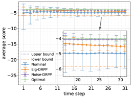
(a) LTI SDS under zero control

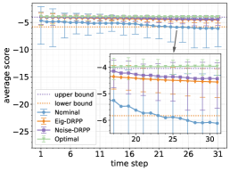
(b) LTV SDS under zero control

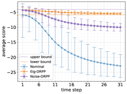
(c) Adversarial SDS under zero control

(d) LTI SDS under LQR control

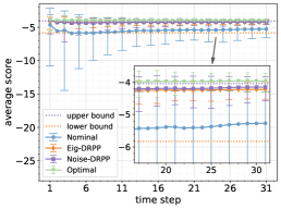
(e) LTV SDS under LQR control

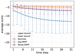
(f) Adversarial SDS under LQR control

Figure 2: Prediction performance of different probabilistic predictors on different SDSs under different control strategies.

VIII-A Experiment Setup

Ambiguity set

Conditioned on a state-control pair $z_{k}$ at time step $k\in\{0,1,\cdots,31\}$, the nominal state evolution function is given as

$$\bar{f}_{k}(\boldsymbol{x}_{k},\boldsymbol{u}_{k})=\begin{pmatrix}1&0.1\\ 0&1\\ \end{pmatrix}\boldsymbol{x}_{k}+\begin{pmatrix}1&0\\ 0&1\end{pmatrix}\boldsymbol{u}_{k},$$

and the uncertainty between $\bar{f}_{k}$ and the true $f_{k}$ is quantified by $\gamma_{0,k}(z_{k})=\min\{0.3\|z_{k}\|_{2},5\}^{2}$. The nominal support, nominal mean and covariance of the noise $\boldsymbol{w}_{k}$ conditioned on $z_{k}$ are

$$\mathcal{W}_{k}=\mathbb{R}^{2},\bar{\mu}_{k}=\begin{pmatrix}0\\ 0\end{pmatrix},\bar{\Sigma}_{k}=\begin{pmatrix}1&0.5\\ 0.5&1.5\end{pmatrix},$$

and the uncertainty between $\bar{\mu}_{k},\bar{\Sigma}_{k}$ and the real $\mu_{k},\Sigma_{k}$ are quantified by $\gamma_{1,k}=0.5$ and $\gamma_{2,k}=3$, respectively. Given the ambiguity set specified above, we simulate the real SDS by randomly choosing one from $\mathcal{I}_{k}$. Although the nominal model is an LTI model, the real model does not have to be LTI. This is because $\mathcal{I}_{k}$ contains linear time-variant (LTV) and even nonlinear time-variant (NTV) models.

Simulation mechanism

In this section, three different simulation mechanisms are conducted, corresponding to LTI, LTV, and adversarial NTV models, respectively.

i) (LTI) Let $\boldsymbol{\alpha}_{1},\boldsymbol{\alpha}_{2}$ be two independent random variables subject to the uniform distribution on $[-1,1]$, and let $\boldsymbol{\alpha}_{3}$ be another independent random variable subject to the uniform distribution on $[-1,1]^{2}$. We randomly generates $\alpha_{i}\sim p_{\boldsymbol{\alpha}_{i}}$ for $i=1,2,3$, then we simulate a LTI SDS as

$$\boldsymbol{x}_{k+1}=\begin{pmatrix}1&0.1+0.3\alpha_{1}\\ 0&1\\ \end{pmatrix}\boldsymbol{x}_{k}+\begin{pmatrix}1&0.3\alpha_{2}\\ 0&1\end{pmatrix}\boldsymbol{u}_{k}+\boldsymbol{w}_{k},$$

where $\boldsymbol{w}_{k}\sim\mathcal{N}\left(0.5\alpha_{3},3\bar{\Sigma}_{k}-0.25\alpha_{3}\alpha_{3}^{\top}\right)$.

ii) (LTV) Similar to the LTI simulation, for each $i=1,2,3$, let $\{\boldsymbol{\alpha}_{i,k}\}_{k=0}^{31}$ be random variables that are independent and identically distributed to $p_{\boldsymbol{\alpha}_{i}}$. We randomly generates $\alpha_{i,k}\sim p_{\boldsymbol{\alpha}_{i,k}}$ for each $i$ and $k$, then we simulate a LTV SDS as

$$\boldsymbol{x}_{k+1}=\begin{pmatrix}1&0.1+0.3\alpha_{1,k}\\ 0&1\\ \end{pmatrix}\boldsymbol{x}_{k}+\begin{pmatrix}1&0.3\alpha_{2,k}\\ 0&1\end{pmatrix}\boldsymbol{u}_{k}+\boldsymbol{w}_{k},$$

where $\boldsymbol{w}_{k}\sim\mathcal{N}(0.5\alpha_{3,k},3\bar{\Sigma}_{k}-0.25\alpha_{3,k}\alpha_{3,k}^{\top})$.

iii) (Adversarial) In this case, the underlying SDS is no longer linear or pre-generated before prediction. It is allowed to adversarially choose an SDS in the ambiguity set at each step such that the prediction performance is minimized. Specifically, at each step, after a predictive pdf has been output by the predictor, the adversarial SDS uses the predictive covariance to choose a worst-case SDS as described in Theorem 4.

Predictors comparison

We study two different control strategies, the zero input and the linear quadratic regulation (LQR). Specifically, the zero input strategy means no control input is imposed, and the LQR control strategy is defined as a standard linear quadratic regulator based on the nominal linear model with $Q$ and $R$ all set as identity matrices. Under each control strategy, we randomly generate 1,000 trajectories starting from the same initial state $x_{0}=[2,1]$ for each of the generation mechanisms. For the LTI and LTV mechanisms, since the ground-truth dynamics are known before prediction, we have an optimal predictor as the least upper bound of prediction performance. At each time step $k$, let the nominal predictor predicts $\bar{p}_{k}\sim\mathcal{N}(\bar{\nu}_{k}+\bar{\mu}_{k},\bar{\Sigma}_{k})$, and the optimal predictor predicts $p_{k}\sim\mathcal{N}(\nu_{k}+\mu_{k},\Sigma_{k})$. Then, we compare the prediction performance among the nominal predictor, Noise-DRPP, Eig-DRPP, and the optimal predictor. For the adversarial mechanism, there is no explicit predefined optimal predictor because the the real SDS depends on the predictor. Therefore, we should compare the prediction performance among the nominal predictor, Noise-DRPP, and Eig-DRPP. In fact, as guaranteed by Theorem 4, when predictors are constrained by the eigenvector restriction, Eig-DRPP is the optimal predictor under this adversarial scenario.

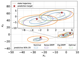
(a) LTI SDS under zero control

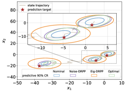
(b) LTV SDS under zero control

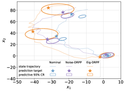
(c) Adversarial SDS under zero control

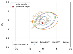
(d) LTI SDS under LQR control

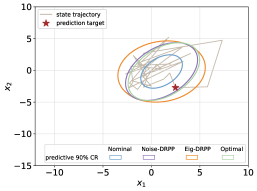
(e) LTV SDS under LQR control

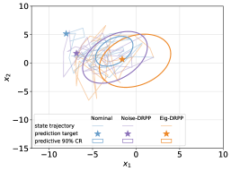
(f) Adversarial SDS under LQR control

Figure 3: Predictive 90% confidence regions of probabilistic predictors for different SDSs under different control strategies.

VIII-B Results and Discussions

In Fig. 2, the prediction performances of different probabilistic predictors on different SDSs under different control strategies are visualized and compared with each other. (a-c) are performances under zero control strategy, and (d-f) are performances under LQR control strategy; the SDSs in (a) and (d) are the same, generated from the LTI mechanism. The SDSs in (b) and (e) are the same, generated from the LTV mechanism; the SDSs in (c) and (f) are the same, generated from the adversarial mechanism. For each SDS, we evaluate the temporal average scores of each predictor at each time step on 1,000 randomly sampled trajectories. At each step, the mean of 1,000 average scores is plotted as a dot, which is an approximation to the expected average score. The 5% and 95% percentiles of these average scores are plotted as an error bar, reflecting how concentrated the average scores are.

Performance advantages

Under each setting of SDS and control strategy, both Noise-DRPP and Eig-DRPP possess larger expected average scores at each time step compared to the nominal predictor. Since the ambiguity set for our simulation does not have too large an uncertainty, the scores of both DRPP predictors are close to the optimal predictor. Additionally, both DRPP predictors have more concentrated average scores at each time step. As the uncertainty of the real underlying SDS increases from LTI to adversarial, the performance gap between the DRPP predictors and the nominal predictor increases.

Upper and lower bounds

When the ambiguity set is not assured to be accurate, we can use the theoretical upper and lower bounds to adjust the ambiguity set, and then improve the performance of DRPP predictors. We provide two simple but efficient rules to adjust the ambiguity set in practice: i) If the expected score of any DRPP predictor is always larger than the upper bound, it means that the true SDS is less adversarial than the worst-case SDS in $\mathcal{I}_{k}$, thus the predictor can use a smaller ambiguity set for better scores. ii) If the expected score of an Eig-DRPP predictor is always smaller than the lower bound, it means that the true SDS is more adversarial than the worst-case SDS in $\mathcal{I}_{k}$, thus the Eig-DRPP predictor can use a larger ambiguity set for better scores.

Influence of control strategies

As we have discussed in Remark 4, when a predictor has no ambiguity of the system’s state evolution function, predicting the states is equivalent to predicting the noises. In this case, the choice of control strategies does not affect any probabilistic predictor. However, when a predictor does have ambiguity of the system’s state evolution function, different control strategies can greatly influence the performance of a probabilistic predictor. Since the ambiguity set at each step directly depends on the state-input pair, different control strategies will lead to quite different state-input trajectories, thus leading to quite different prediction performances. We can observe this phenomenon by comparing (a-c) with (d-f) in Fig. 2 respectively. An intuitive explanation is that the LQR control strategy regulates the system states towards the neighborhoods of $0$, where the ambiguity of one-step state evolution is smaller than other states, thus the DRPP predictors perform better.

VIII-C Application: Predict Robust Confidence Regions

An immediate application of probabilistic prediction is to predict high-probability confidence regions for future states. Since the predictive pdfs of both Noise-DRPP and Eig-DRPP are Gaussian, one can easily derive an elliptical $\beta$-confidence region for any $\beta\in(0,1)$. In Fig. 3, we have visualized the predictive 90% confidence regions for each predictor at certain time steps of a randomly generated trajectory.

Visualizing the behaviors of different probabilistic predictors on a trajectory, one can intuitively explain why DRPP predictors outperform the nominal predictor. The nominal predictor is overly confident, where the predictive pdfs are always too sharp to enclose the future states in their 90% CRs. In contrast, DRPP predictors have taken the ambiguity of noises into account, whose CRs are more robust to contain the prediction targets most of the time. If we further compare Noise-DRPP with Eig-DRPP, it seems that Eig-DRPP is more intelligent in adaptively changing the ellipses’ shapes. This is because Eig-DRPP has also considered the ambiguity of one-step state evolution, and the eigenvalues of predictive covariances are attained based on minimax optimization.

IX Conclusion

This paper presented a distributionally robust probabilistic prediction (DRPP) framework to address the challenges of predicting future states in stochastic dynamical systems (SDSs) with incomplete and imprecise distributional information. The proposed DRPP framework ensures robust performance by designing predictors that account for the worst-case scenarios over a predefined ambiguity set of SDSs. To overcome the inherent intractability of optimizing over function spaces, we reformulated the original functional-maximin problem into an equivalent convex-nonconcave minimax problem in Euclidean spaces.

While achieving the global optimal solution remains computationally prohibitive, we developed two practical suboptimal predictors: Noise-DRPP, obtained by relaxing the inner constraints, and Eig-DRPP, derived from relaxing the outer constraints. An explicit upper bound on the optimality gap between Eig-DRPP and the global optimal predictor was also established, providing theoretical guarantees on the quality of the suboptimality. Furthermore, leveraging the theoretical results, we proposed practical guidelines to assess and refine the size of the ambiguity set, balancing robustness and conservatism. Numerical simulations demonstrated the effectiveness and practicality of the proposed predictors across various SDSs, highlighting their ability to deliver distributionally robust probabilistic predictions under different settings.

The DRPP framework developed in this work is promising for future exploration of computationally efficient predictors under different types of scoring rules and ambiguity sets.

Appendix A Discussion on Canonicalization

If we align $p_{\boldsymbol{\xi}_{k}}$ with $p_{\boldsymbol{w}_{k}}$ and optimize over $p_{\boldsymbol{w}_{k}}$, i.e., $\inf_{\nu_{k},\mu_{k},p_{\boldsymbol{w}_{k}}}\mathbb{E}_{w\sim p_{\boldsymbol{w}_{k}}}\log[\hat{p}_{k}(w+\nu_{k})]$, the Lagrange function would have been

$$L(p_{\boldsymbol{w}_{k}},\nu_{k},\mu_{k},r,q,Q_{1},Q_{2},P_{1},p_{1},s_{1},P_{2},p_{2},s_{2})$$

$$:= \langle p_{\boldsymbol{w}_{k}},\log\hat{p}_{k}(w\!+\!\nu_{k})\rangle+r\left[\langle p_{\boldsymbol{w}_{k}},1\rangle\!-\!1\right]+q^{\top}\!\left[\langle p_{\boldsymbol{w}_{k}},w\rangle\!-\!\mu\right]$$

$$+Q_{1}\cdot\left[\langle p_{\boldsymbol{w}_{k}},(w-\bar{\mu}_{k})(w-\bar{\mu}_{k})^{\top}\rangle-\gamma_{2,k}\bar{\Sigma}_{k}\right]$$

$$-Q_{2}\cdot\left[\langle p_{\boldsymbol{w}_{k}},(w-\bar{\mu}_{k})(w-\bar{\mu}_{k})^{\top}\rangle-\gamma_{3,k}\bar{\Sigma}_{k}\right]$$

$$-P_{1}\cdot\bar{\Sigma}_{k}-2p_{1}^{\top}(\mu_{k}-\bar{\mu}_{k})-s_{1}\gamma_{1,k}$$

$$-P_{2}\cdot\bar{\Sigma}_{k}-2p_{2}^{\top}(\nu_{k}-\bar{\nu}_{k})-s_{2}\gamma_{0,k}(z_{k}).$$

However, minimizing the Lagrange function over $p_{\boldsymbol{w}_{k}}$ and $\nu_{k}$ cannot lead to further useful analysis. On the one hand, if $p_{\boldsymbol{w}_{k}}$ is minimized before $\nu_{k}$, it will lead to constraints $\log[\hat{p}_{k}(w+\nu_{k})]+r+q^{\top}w+w^{\top}(Q_{1}-Q_{2})w\geq 0\;\forall w\in\mathbb{R}^{d_{x}}$. Then the minimization over $\nu_{k}$ is constrained by these constraints, which makes it impossible to derive explicit expression for an optimal $\nu_{k}^{*}$. On the other hand, minimizing $\nu_{k}$ before $p_{\boldsymbol{w}}$ also fails to derive an explicit expression for the optimal $\nu_{k}^{*}$ because the form of $\hat{p}_{k}$ remains undetermined. Therefore, we should not formulate the inner minimization over $p_{\boldsymbol{w}_{k}}$.

Appendix B Duality of Problem (8)

Proof.

The Lagrange function for (8) is defined as

$$L(p_{\boldsymbol{\xi}_{k}},\nu_{k},\mu_{k},r,q,Q_{1},Q_{2},P_{1},p_{1},s_{1},P_{2},p_{2},s_{2})$$

$$:= \langle p_{\boldsymbol{\xi}_{k}},\log\hat{p}_{k}(\xi)\rangle+r\left[\langle p_{\boldsymbol{\xi}_{k}},1\rangle\!-\!1\right]+q^{\top}\!\left[\langle p_{\boldsymbol{\xi}_{k}},\xi\rangle\!-\!\mu_{k}\!-\!\nu_{k}\right]$$

$$+Q_{1}\cdot\left[\langle p_{\boldsymbol{\xi}_{k}},(\xi-\nu_{k}-\bar{\mu}_{k})(\xi-\nu_{k}-\bar{\mu}_{k})^{\top}\rangle-\gamma_{2,k}\bar{\Sigma}_{k}\right]$$

$$-Q_{2}\cdot\left[\langle p_{\boldsymbol{\xi}},(\xi-\nu_{k}-\bar{\mu}_{k})(\xi-\nu_{k}-\bar{\mu}_{k})^{\top}\rangle-\gamma_{3,k}\bar{\Sigma}_{k}\right]$$

$$-P_{1}\cdot\bar{\Sigma}_{k}-2p_{1}^{\top}(\mu-\bar{\mu}_{k})-s_{1}\gamma_{1,k}$$

$$-P_{2}\cdot I-2p_{2}^{\top}(\nu_{k}-\bar{\nu}_{k})-s_{2}\gamma_{0,k}(z_{k}).$$

where the Lagrange multipliers satisfy $Q_{1}\succeq 0,Q_{2}\succeq 0$ and $\begin{bmatrix}P_{i}&p_{i}\\ p_{i}^{\top}&s_{i}\end{bmatrix}\succeq 0$ for $i\in\{1,2\}$. Let $\mathcal{M}_{+}$ be the set of positive measures on $\mathbb{R}^{d_{x}}$. Minimizing over $p_{\boldsymbol{\xi}_{k}}\in\mathcal{M}_{+}$, $\mu_{k}\in\mathbb{R}^{d_{x}}$, and $\nu_{k}\in\mathbb{R}^{d_{x}}$ we have

$$\inf_{p_{\boldsymbol{\xi}_{k}}\in\mathcal{M}_{+},\mu_{k},\nu_{k}}\!\!\!\!\!\!\!L(p_{\boldsymbol{\xi}_{k}},\nu_{k},\mu_{k},r,q,Q_{1},Q_{2},P_{1},p_{1},s_{1},P_{2},p_{2},s_{2})$$

$$= \inf_{p_{\boldsymbol{\xi}_{k}}\in\mathcal{M}_{+},\mu_{k},\nu_{k}}\langle p_{\boldsymbol{\xi}_{k}},\log\hat{p}_{k}(\xi)+r+q^{\top}\xi+\xi^{\top}\!(Q_{1}\!-\!Q_{2})\xi\rangle$$

$$-(q+2p_{1})^{\top}\mu_{k}-(q+2p_{2})^{\top}\nu_{k}-(\gamma_{2,k}Q_{1}-\gamma_{3,k}Q_{2})\!\cdot\!\bar{\Sigma}_{k}$$

$$-(\nu_{k}+2\mu_{k}-\bar{\mu}_{k})^{\top}(Q_{1}-Q_{2})(\nu_{k}+\bar{\mu}_{k})-r$$

$$-P_{1}\!\cdot\!\bar{\Sigma}_{k}+2p_{1}^{\top}\bar{\mu}_{k}-s_{1}\gamma_{1,k}-P_{2}\!\cdot\!I+2p_{2}^{\top}\bar{\mu}_{k}-s_{2}\gamma_{0,k}(z_{k})$$

$$\overset{(i)}{=} \inf_{\mu_{k},\nu_{k}}-(q\!+\!2p_{1})^{\top}\!\mu_{k}\!-\!(q\!+\!2p_{2})^{\top}\nu_{k}\!-\!(\gamma_{2,k}Q_{1}\!-\!\gamma_{3,k}Q_{2})\!\cdot\!\bar{\Sigma}_{k}$$

$$-(\nu_{k}+2\mu_{k}-\bar{\mu}_{k})^{\top}(Q_{1}-Q_{2})(\nu_{k}+\bar{\mu}_{k})-r$$

$$-P_{1}\!\cdot\!\bar{\Sigma}_{k}+2p_{1}^{\top}\bar{\mu}_{k}-s_{1}\gamma_{1,k}-P_{2}\!\cdot\!I+2p_{2}^{\top}\bar{\nu}_{k}-s_{2}\gamma_{0,k}(z_{k})$$

$$\overset{(ii)}{=} \!-\!r\!+\!\bar{\mu}_{k}^{\top}\!(Q_{1}\!-\!Q_{2})\bar{\mu}_{k}\!-\!(\gamma_{2,k}Q_{1}\!-\!\gamma_{3,k}Q_{2}\!+\!P_{1})\!\cdot\!\bar{\Sigma}_{k}\!-P_{2}\cdot I$$

$$+\!2p_{1}^{\top}\!\bar{\mu}_{k}\!-\!s_{1}\gamma_{1,k}+\!2p_{2}^{\top}\!\bar{\mu}_{k}\!-\!s_{2}\gamma_{0,k}(z_{k})-(q+2p_{2})^{\top}\nu_{k}$$

$$-\nu_{k}^{\top}(Q_{1}-Q_{2})\nu_{k}.$$

Equation $(i)$ holds when $\log\hat{p}_{k}(\xi)+r+q^{\top}\xi+\xi^{\top}(Q_{1}-Q_{2})\xi\geq 0\;\forall\xi\in\mathbb{R}^{d_{x}}$, otherwise there is $\inf_{p_{\boldsymbol{\xi}_{k}}\in\mathcal{M}_{+},\mu_{k}}L$ equals $-\infty$. Equation $(ii)$ holds because

$$\inf_{\mu_{k},\nu_{k}}-(q+2p_{1})^{\top}\mu_{k}-(q+2p_{2})^{\top}\nu_{k}-\bar{\mu}_{k}^{\top}(Q_{1}-Q_{2})\bar{\mu}_{k}$$

$$-(\nu_{k}+2\mu_{k}-\bar{\mu}_{k})^{\top}(Q_{1}-Q_{2})(\nu_{k}+\bar{\mu}_{k})$$

$$= \inf_{\nu_{k}}\inf_{\mu_{k}}-[q+2p_{1}+2(Q_{1}-Q_{2})(\nu_{k}+\bar{\mu}_{k})]^{\top}\mu_{k}$$

$$\qquad-(q+2p_{2})^{\top}\nu_{k}-\nu_{k}^{\top}(Q_{1}-Q_{2})\nu_{k}$$

$$= \inf_{\nu_{k}}-(q+2p_{2})^{\top}\nu_{k}-\nu_{k}^{\top}(Q_{1}-Q_{2})\nu_{k}$$

$$\text{ s.t.}q+2p_{1}+2(Q_{1}-Q_{2})(\nu_{k}+\bar{\mu}_{k})=0$$

Combining those conditions and the previous multipliers’ constraints, we have the dual form completed. ∎

Appendix C Proof of Theorem 1

Proof.

Step I. We leverage the separable structure of $\mathbf{D}_{1}$ to reformulate the problem. For ease of notation, we use the $\kappa$ to summarize all the Lagrange multipliers except for $r$, i.e.,

$$\kappa=(q,Q_{1},Q_{2},P_{1},p_{1},s_{1},P_{2},p_{2},s_{2}).$$

First, the objective function can be separated as $G(r,\kappa)=-r+g(\kappa)$ where $g(\kappa)=\bar{\mu}_{k}^{\top}\!(Q_{1}\!-\!Q_{2})\bar{\mu}_{k}-(\gamma_{2,k}Q_{1}-\gamma_{3,k}Q_{2}+P_{1})\cdot\bar{\Sigma}_{k}-P_{2}\cdot I+2p_{1}^{\top}\bar{\mu}_{k}-s_{1}\gamma_{1,k}+2p_{2}^{\top}\bar{\nu}_{k}-s_{2}\gamma_{0,k}\|z_{k}\|^{2}_{2}-(q+2p_{2})^{\top}\nu_{k}-\nu_{k}^{\top}(Q_{1}-Q_{2})\nu_{k}$. Second, only the second constraint concerns $r$. Therefore, given any group of feasible $\kappa$ satisfying the last three constraints in $\mathbf{D}_{1}$, the optimizing over $\hat{p}_{k}$ and $r$ is equivalent to solving the following problem:

$$\sup_{\hat{p}_{k},r}-r+g(\kappa)$$ (17)

$$\text{s.t.}\left\{\begin{aligned} &\mathbb{E}_{\xi\sim\hat{p}_{k}}1=1,\quad\hat{p}_{k}(\xi)\geq 0\;\forall\xi\in\mathbb{R}^{d_{x}}\\ &\xi^{\top}\!(Q_{1}\!-\!Q_{2})\xi\!+\!\xi^{\top}\!q\!+\!r\!+\!\log\hat{p}_{k}(\xi)\!\geq\!0\,\forall\xi\!\in\!\mathbb{R}^{d_{x}}.\end{aligned}\right.$$

Step II. We exploit the last constraint in (17) to analyze the lower bound of $r$. Notice that

$$1 =\int_{\mathbb{R}^{d_{x}}}\hat{p}_{k}(\xi)\mathrm{d}\xi$$ (18)

$$\geq\int_{\mathbb{R}^{d_{x}}}\exp\{-\xi^{\top}\!(Q_{1}-Q_{2})\xi-\xi^{\top}q-r\}\mathrm{d}\xi,$$

one immediately has that $Q_{1}-Q_{2}$ is semi-definite positive. Because $Q_{1}$ and $Q_{2}$ are both semi-definite, we have $Q_{1}-Q_{2}$ is symmetric and there exists an orthogonal matrix $U\in\mathbb{R}^{d_{x}\times d_{x}}$ and an diagonal matrix $D=\operatorname{diag}(\lambda_{1},\ldots,\lambda_{d_{x}})$ such that $Q_{1}-Q_{2}=UDU^{\top}$. Then we have

$$\int_{\mathbb{R}^{d_{x}}}\exp\{-\xi^{\top}(Q_{1}-Q_{2})\xi-\xi^{\top}q-r\}\mathrm{d}\xi$$

$$= \int_{\mathbb{R}^{d_{x}}}\exp\{-\xi^{\top}UDU^{\top}\xi-\xi^{\top}q-r\}\mathrm{d}\xi$$

$$= \int_{\mathbb{R}^{d_{x}}}\exp\{-\tilde{\xi}^{\top}D\tilde{\xi}-\tilde{\xi}^{\top}\tilde{q}-r\}\operatorname{det}(U)\mathrm{d}\tilde{\xi}$$

$$= e^{-r}\operatorname{det}(U)\prod_{i=1}^{d_{x}}\int_{\mathbb{R}}\exp\{-\tilde{\xi}_{(i)}^{2}\lambda_{i}-\tilde{\xi}_{(i)}\tilde{q}_{(i)}\}\mathrm{d}\tilde{\xi}_{(i)},$$

where the second equation follows by letting $\tilde{\xi}=U^{\top}\xi$. If there is an index $j\in\{1,\ldots,d_{x}\}$ such that $\lambda_{j}<0$, then $\int_{\mathbb{R}}\exp\{-\tilde{\xi}^{2}_{(i)}\lambda_{j}-\tilde{\xi}_{(j)}\tilde{q}_{(j)}\}\mathrm{d}\tilde{\xi}_{(j)}=\infty$, which contradicts (18). It follows that $r$ can be lower bounded by $r^{*}:=\log\left[\int_{\mathbb{R}^{d_{x}}}\!\!\exp\{-\xi^{\top}\!(Q_{1}-Q_{2})\xi-\xi^{\top}q\}\mathrm{d}\xi\right]$, because

$$1\geq\int_{\mathbb{R}^{d_{x}}}\!\!\exp\{-\xi^{\top}\!(Q_{1}-Q_{2})\xi-\xi^{\top}q-r\}\mathrm{d}\xi$$ (19)

$$\Rightarrow e^{r}\geq\int_{\mathbb{R}^{d_{x}}}\!\!\exp\{-\xi^{\top}\!(Q_{1}-Q_{2})\xi-\xi^{\top}q\}\mathrm{d}\xi$$

$$\Rightarrow r\geq\log\left[\int_{\mathbb{R}^{d_{x}}}\!\!\exp\{-\xi^{\top}\!(Q_{1}-Q_{2})\xi-\xi^{\top}q\}\mathrm{d}\xi\right].$$

Step III. We use the condition that makes (19) equal to obtain the optimality condition. Notice that the equality of (19) holds only when there is $\hat{p}_{k}(\xi)=\exp\{-\xi^{\top}\!(Q_{1}-Q_{2})\xi-\xi^{\top}q-r^{*}\}$ for $\xi\in\mathbb{R}^{d_{x}}$ almost everywhere. Therefore, given any feasible $\kappa$, the objective function $-r+g(\kappa)$ in problem (17) can only attain its maximum when $\hat{p}_{k}$ is a Gaussian distribution almost everywhere.

Finally, considering that the objective of $\mathbf{D}_{2}$ can be reformulated as $\sup_{\kappa}\sup_{\hat{p}_{k},r}G(r,\kappa)$, and a necessary optimal condition for the inner optimization is that $\hat{p}_{k}$ is subject to Gaussian almost everywhere, we have the proof completed. ∎

Appendix D Derivation of (10)

Proof.

Facilitated by Theorem 1, we can first parameterize $\hat{p}_{k}$ by $\hat{\mu}_{k}\in\mathbb{R}^{d_{x}}$ and $\hat{\Sigma}_{k}\in\mathbb{R}^{d_{x}}$ such that

$$\hat{p}_{k}(\xi)\!=\!\frac{1}{\sqrt{(2\pi)^{d_{x}}\operatorname{det}(\hat{\Sigma}_{k})}}\exp\!\left[\!-\frac{1}{2}(\xi\!-\!\hat{\mu}_{k})^{\top}\!{\hat{\Sigma}_{k}}^{-1}(\xi\!-\!{\hat{\mu}_{k}})\right].$$

Substituting it into the constraints of $\mathbf{D}_{1}$, there is

$$\xi^{\top}(Q_{1}-Q_{2})\xi+\xi^{\top}q+r-\frac{1}{2}\left[d_{x}\log(2\pi)+\log\operatorname{det}(\hat{\Sigma}_{k})\right]$$

$$-\frac{1}{2}(\xi-\hat{\mu}_{k})^{\top}{\hat{\Sigma}_{k}}^{-1}(\xi-\hat{\mu}_{k})=0\quad\forall\xi\in\mathbb{R}^{d_{x}}.$$

Then we have $Q_{1}-Q_{2}=\frac{1}{2}\hat{\Sigma}_{k}^{-1}$, $q=-\hat{\Sigma}^{-1}_{k}\hat{\mu}_{k}$, and $r=\frac{1}{2}\left[d_{x}\log(2\pi)+\log\operatorname{det}(\hat{\Sigma}_{k})+\hat{\mu}_{k}^{\top}\hat{\Sigma}_{k}^{-1}\hat{\mu}_{k}\right]$. Substituting these equations and the parameterized $\hat{p}_{k}$ into the objective of problem $\mathbf{D}_{1}$, we get

$$G(r,q,Q_{1},Q_{2},P_{1},p_{1},s_{1},P_{2},p_{2},s_{2})$$

$$= -\frac{1}{2}\left[d_{x}\log(2\pi)+\log\operatorname{det}(\hat{\Sigma}_{k})\right]$$

$$-P_{2}\cdot I-s_{1}\gamma_{1,k}+2p_{2}^{\top}(\bar{\nu}_{k}+\bar{\mu}_{k}-\hat{\mu}_{k})-s_{2}\gamma_{0,k}\|z_{k}\|^{2}_{2}$$

$$+2(2p_{2}-p_{1})^{\top}\hat{\Sigma}_{k}p_{1}-(\gamma_{2,k}Q_{1}\!-\!\gamma_{3,k}Q_{2}\!+\!P_{1})\!\cdot\!\bar{\Sigma}_{k}$$

$$= \!-\!\frac{1}{2}d_{x}\log(2\pi)\!+\!\frac{1}{2}\log\operatorname{det}(\hat{\Sigma}_{k}^{-1})\!-\!(\gamma_{2,k}Q_{1}\!-\!\gamma_{3,k}Q_{2})\!\cdot\!\bar{\Sigma}_{k}$$

$$-P_{1}\!\cdot\!\bar{\Sigma}_{k}-P_{2}\!\cdot\!I-s_{1}\gamma_{1,k}-s_{2}\gamma_{0,k}\|z_{k}\|^{2}_{2}$$

$$-2p_{2}^{\top}(\hat{\mu}_{k}-\bar{\mu}_{k}-\bar{\nu}_{k})+2p_{1}^{\top}\!\hat{\Sigma}_{k}(2p_{2}\!-\!p_{1}).$$

Substituting the above equations into the problem $\mathbf{D}_{1}$, we have the problem (10) derived. ∎

Appendix E Proof of Lemma 1

Proof.

Since the objective function is linear with respect to $\Sigma_{k}$ and the second constraint provides an upper bound for it, one immediately has the worst-case covariance should satisfy that

$$\Sigma_{k}^{*}=\gamma_{2,k}\bar{\Sigma}_{k}-(\mu_{k}-\bar{\mu}_{k})(\mu_{k}-\bar{\mu}_{k})^{\top}.$$

Let $a=\mu_{k}-\bar{\mu}_{k},b=\nu_{k}-\bar{\nu}_{k},c=\bar{\mu}_{k}+\bar{\nu}_{k}-\hat{\mu}_{k}$, problem $\mathbf{P}_{2}$ can be further equivalent to

$$\inf_{\hat{\Sigma}_{k}^{-1},c}\sup_{a,b} \;-\log\operatorname{det}(\hat{\Sigma}_{k}^{-1})+\gamma_{2,k}\bar{\Sigma}_{k}\!\cdot\!\hat{\Sigma}_{k}^{-1}$$ (20)

$$\;+\|a+b+c\|_{\hat{\Sigma}_{k}^{-1}}^{2}-\|a\|_{\hat{\Sigma}_{k}^{-1}}^{2}$$

s.t. $$\;\|a\|_{\bar{\Sigma}_{k}^{-1}}^{2}\leq\gamma_{1,k},\|b\|_{2}^{2}\leq\gamma_{0,k}(z_{k}).$$

Suppose $(a^{*},b^{*})\in\arg\max_{a,b}\left\{\|a+b\|_{\hat{\Sigma}^{-1}}^{2}-\|a\|_{\hat{\Sigma}^{-1}}^{2}\right\}$, we have $(-a^{*},-b^{*})$ can also attain the maximum. Then we have

$$\max_{a,b}\|a+b+c\|^{2}_{\hat{\Sigma}_{k}^{-1}}-\|a\|^{2}_{\hat{\Sigma}_{k}^{-1}}$$

$$\geq \max\left\{\|a^{*}+b^{*}+c\|^{2}_{\hat{\Sigma}_{k}^{-1}}-\|a^{*}\|^{2}_{\hat{\Sigma}_{k}^{-1}},\right.$$

$$\left.\qquad\|-a^{*}-b^{*}+c\|^{2}_{\hat{\Sigma}_{k}^{-1}}-\|-a^{*}\|^{2}_{\hat{\Sigma}_{k}^{-1}}\right\}$$

$$= \|a^{*}+b^{*}\|^{2}_{\hat{\Sigma}_{k}^{-1}}-\|a^{*}\|^{2}_{\hat{\Sigma}_{k}^{-1}}+\|c\|_{\hat{\Sigma}_{k}}^{-1}$$

$$+2\max\left\{\langle c,a^{*}+b^{*}\rangle_{\hat{\Sigma}_{k}^{-1}},-\langle c,a^{*}+b^{*}\rangle_{\hat{\Sigma}_{k}^{-1}}\right\}$$

$$\geq \|a^{*}+b^{*}\|^{2}_{\hat{\Sigma}_{k}^{-1}}-\|a^{*}\|^{2}_{\hat{\Sigma}_{k}^{-1}}$$

where the last inequality is strict when $c\neq 0$. Therefore, we have $c^{*}=\arg\min_{c}\max_{a,b}\|a+b+c\|^{2}_{\hat{\Sigma}_{k}^{-1}}-\|a\|^{2}_{\hat{\Sigma}_{k}^{-1}}=0$, which means that $\hat{\mu}^{*}_{k}=\bar{\mu}_{k}+\bar{\nu}_{k}$.

∎

Appendix F Duality of the moment problem (14)

Proof.

The Lagrange function for (14) is defined as

$$L(p_{\boldsymbol{w}_{k}},\mu_{k},r,q,Q_{1},Q_{2},P,p,s)$$

$$:= \langle p_{\boldsymbol{w}_{k}},\log\hat{p}(w\!+\!\bar{\nu}_{k})\rangle\!+\!r\left[\langle p_{\boldsymbol{w}_{k}},1\rangle\!-\!1\right]\!+\!q^{\top}\!\left[\langle p_{\boldsymbol{w}_{k}},w\rangle\!-\!\mu_{k}\right]$$

$$+Q_{1}\cdot\left[\langle p_{\boldsymbol{w}_{k}},(w-\bar{\mu}_{k})(w-\bar{\mu}_{k})^{\top}\rangle-\gamma_{2,k}\bar{\Sigma}_{k}\right]$$

$$-Q_{2}\cdot\left[\langle p_{\boldsymbol{w}_{k}},(w-\bar{\mu}_{k})(w-\bar{\mu}_{k})^{\top}\rangle-\gamma_{3,k}\bar{\Sigma}_{k}\right]$$

$$-P\cdot\bar{\Sigma}_{k}-2p^{\top}(\mu-\bar{\mu}_{k})-s\gamma_{1,k},$$

where the Lagrange multipliers satisfy $Q_{1}\succeq 0,Q_{2}\succeq 0$ and $\begin{bmatrix}P&p\\ p^{\top}&s\end{bmatrix}\succeq 0$. Let $\mathcal{M}_{+}$ be the set of positive measures on $\mathbb{R}^{d_{x}}$. Minimizing over $p_{\boldsymbol{w}_{k}}\in\mathcal{M}_{+}$ and $\mu_{k}\in\mathbb{R}^{d_{x}}$, one has

$$\inf_{p_{\boldsymbol{w}_{k}}\in\mathcal{M}_{+},\mu_{k}}L(p_{\boldsymbol{w}_{k}},\mu_{k},r,q,Q_{1},Q_{2},P,p,s)$$

$$= \inf_{p_{\boldsymbol{w}_{k}}\in\mathcal{M}_{+},\mu_{k}}\!\!\!\!\langle p_{\boldsymbol{w}_{k}},\log\hat{p}(w\!+\!\bar{\nu}_{k})\!+\!r\!+q\!^{\top}\!w\!+\!w^{\top}\!(Q_{1}\!-\!Q_{2})w\rangle$$

$$-\left[q+2(Q_{1}-Q_{2})\bar{\mu}_{k}+2p\right]^{\top}\mu_{k}-r+\bar{u}_{k}^{\top}(Q_{1}-Q_{2})\bar{u}_{k}$$

$$-(\gamma_{2,k}Q_{1}-\gamma_{3,k}Q_{2}+P)\!\cdot\!\bar{\Sigma}_{k}+2p^{\top}\bar{\mu}_{k}-s\gamma_{1,k}$$

$$= -r\!+\!\bar{u}_{k}^{\top}\!(Q_{1}\!-\!Q_{2})\bar{u}_{k}\!-\!(\gamma_{2,k}Q_{1}\!-\!\gamma_{3,k}Q_{2}\!+\!P)\!\cdot\!\bar{\Sigma}_{k}\!+\!2p^{\top}\!\bar{\mu}_{k}$$

$$-\!s\gamma_{1,k},$$

where the second equality holds when $\log\hat{p}(w+\bar{\nu}_{k})+r+q^{\top}w+w^{\top}(Q_{1}-Q_{2})w\geq 0\;\forall w\in\mathbb{R}^{d_{x}}$ and $q+2(Q_{1}-Q_{2})+2p=0$ hold simultaneously, otherwise there is $\inf_{p_{\boldsymbol{w}}\in\mathcal{M}_{+},\mu}L=-\infty$. Combining these two conditions and the previous multipliers’ constraints, we have attained the dual problem $\mathbf{D}_{2}$. ∎

Appendix G Proof of Theorem 2

Proof.

The proof is organized in three parts: first, we use Theorem 1 to parameterize $\hat{p}_{k}$ by Gaussian distribution $\mathcal{N}(\hat{\mu}_{k},\hat{\Sigma}_{k})$ and reformulate the dual problem $\mathbf{D}_{2}$ to a finite-dimensional optimization; second, we solve the optimal predictive pdf $\hat{p}^{*}_{k}\sim\mathcal{N}(\hat{\mu}^{*}_{k},\hat{\Sigma}^{*}_{k})$; third, we substitute $\hat{p}^{*}_{k}$ into the original problem $\mathbf{P}_{1}$ to obtain the worst-case SDS $\Phi^{*}_{k}$ by solving the inner minimization.

Step I. Using the necessary optimality condition for $\hat{p}_{k}$, we can parameterize $\hat{p}_{k}$ by $\hat{\mu}_{k}\in\mathbb{R}^{d_{x}}$ and $\hat{\Sigma}_{k}\in\mathbb{R}^{d_{x}\times d_{x}}$ such that

$$\hat{p}_{k}(w\!+\!\bar{\nu}_{k})\!=\!\frac{\exp\!\left[\!-\frac{1}{2}(w\!-\!\hat{\mu}_{k})^{\top}\!{\hat{\Sigma}_{k}}^{-1}(w\!-\!{\hat{\mu}_{k}})\right]}{\sqrt{(2\pi)^{d_{x}}\operatorname{det}(\hat{\Sigma}_{k})}}.$$

Moreover, from the constraint $w^{\top}\!(Q_{1}-Q_{2})w+w^{\top}q+r+\log\hat{p}(w+\bar{\nu}_{k})\geq 0\;\forall w\in\mathbb{R}^{d_{x}}$, we get

$$w^{\top}(Q_{1}\!-\!Q_{2})w+w^{\top}\!q+r-\frac{1}{2}\left[d_{x}\log(2\pi)\!+\!\log\operatorname{det}(\hat{\Sigma}_{k})\right]$$

$$-\frac{1}{2}(w-\hat{\mu}_{k})^{\top}{\hat{\Sigma}_{k}}^{-1}(w-\hat{\mu}_{k})=0\quad\forall w\in\mathbb{R}^{d_{x}},$$

which indicates that $Q_{1}-Q_{2}=\frac{1}{2}\hat{\Sigma}_{k}^{-1}$, $q=-\hat{\Sigma}_{k}^{-1}\hat{\mu}_{k}$, and $r=\frac{1}{2}\left[d_{x}\log(2\pi)+\log\operatorname{det}(\hat{\Sigma}_{k})+\hat{\mu}_{k}^{\top}\hat{\Sigma}_{k}^{-1}\hat{\mu}_{k}\right]$. Next, from the constraint $q+2(Q_{1}-Q_{2})\bar{\mu}_{k}+2p=0$ one can get $p=\frac{1}{2}\hat{\Sigma}_{k}^{-1}(\hat{\mu}_{k}-\bar{\mu}_{k})$. Substituting the parameterized $\hat{p}_{k}$ and the above equations into problem $\mathbf{D}_{2}$, there is

$$G(r,q,Q_{1},Q_{2},P,p,s)=-\frac{1}{2}\left[d_{x}\log(2\pi)+\log\operatorname{det}(\hat{\Sigma}_{k})\right]$$

$$\quad\;-\frac{1}{2}\hat{\mu}_{k}^{\top}\!{\hat{\Sigma}_{k}}^{-1}\hat{\mu}_{k}+\bar{\mu}_{k}^{\top}(Q_{1}-Q_{2})\bar{\mu}_{k}+\bar{\mu}_{k}^{\top}\hat{\Sigma}_{k}^{-1}(\hat{\mu}_{k}-\bar{\mu}_{k})$$

$$\quad\;-(\gamma_{2,k}Q_{1}-\gamma_{3,k}Q_{2}+P)\cdot\bar{\Sigma}_{k}-s\gamma_{1,k}$$

$$=-\frac{1}{2}\left[d_{x}\log(2\pi)\!-\!\frac{1}{2}\log\operatorname{det}(\hat{\Sigma}_{k}^{-1})\!+\!\|\hat{\mu}_{k}\!-\!\bar{\mu}_{k}\|_{\hat{\Sigma}_{k}^{-1}}^{2}\right]$$

$$\quad\;-(\gamma_{2,k}Q_{1}-\gamma_{3,k}Q_{2}+P)\cdot\bar{\Sigma}_{k}-s\gamma_{1,k}.$$

As a result, $\mathbf{D}_{2}$ can be transformed into a finite-dimensional optimization problem as follows:

$$\sup_{\hat{\mu}_{k},\hat{\Sigma}_{k},Q_{1},Q_{2},P,p,s}\!\!-\frac{1}{2}d_{x}\log(2\pi)\!+\!\frac{1}{2}\log\operatorname{det}(\hat{\Sigma}_{k}^{-1})\!-\!s\gamma_{1,k}$$ (21)

$$-\frac{1}{2}\|\hat{\mu}_{k}\!-\!\bar{\mu}_{k}\|_{\hat{\Sigma}_{k}^{-1}}^{2}\!-\!(\gamma_{2,k}Q_{1}\!-\!\gamma_{3,k}Q_{2}\!+\!P)\!\cdot\!\bar{\Sigma}_{k}$$

$$\text{s.t.}\left\{\begin{aligned} &Q_{1}\succeq 0,Q_{2}\succeq 0,Q_{1}-Q_{2}=\frac{1}{2}\hat{\Sigma}_{k}^{-1},\hat{\Sigma}_{k}\succ 0\\ &\left[\begin{array}[]{cc}P&p\\ p^{\top}&s\end{array}\right]\succeq 0,p=\frac{1}{2}\hat{\Sigma}_{k}^{-1}(\hat{\mu}_{k}-\bar{\mu}_{k}).\end{aligned}\right.$$

Step II. Notice that the constraint $\hat{\Sigma}_{k}\succ 0$ and the relationship $p=\frac{1}{2}\hat{\Sigma}_{k}^{-1}(\hat{\mu}_{k}-\bar{\mu}_{k})$ reveals that $p$ and $\hat{\mu}_{k}$ are one-on-one, one can optimize on either of them. In this proof, we choose to maximize over $p$ and substitute $\hat{\mu}_{k}$ in the objective by $p$. Next, notice that the constraints for $Q_{1},Q_{2}$ only depend on $\hat{\Sigma}_{k}$, and it can be separated from the constraints for $P,p,s$, we can first maximize over $Q_{1}$ and $Q_{2}$, then over $P,p,s$, finally over $\hat{\Sigma}$. In other words, the objective of problem (21) can be reformulated as

$$\sup_{\hat{\Sigma}_{k}}\sup_{P,p,s}\sup_{Q_{1},Q_{2}}\!\!-\frac{1}{2}d_{x}\log(2\pi)\!+\!\frac{1}{2}\log\operatorname{det}(\hat{\Sigma}^{-1})$$ (22)

$$-2p^{\top}\!\hat{\Sigma}p\!-\!(\gamma_{2,k}Q_{1}\!-\!\gamma_{3,k}Q_{2}\!+\!P)\!\cdot\!\bar{\Sigma}_{k}-\!s\gamma_{1,k}.$$

The solution of the first maximization is $Q_{1}^{*}=\frac{1}{2}\hat{\Sigma}_{k}^{-1},Q_{2}^{*}=0$ because

$$Q_{1}^{*}= \arg\max_{Q_{1}\succeq\frac{1}{2}\hat{\Sigma}_{k}^{-1}}-((\gamma_{2,k}-\gamma_{3,k})Q_{1}+\frac{\gamma_{3,k}}{2}\hat{\Sigma}_{k}^{-1})\cdot\bar{\Sigma}_{k}$$

$$= \arg\max_{Q_{1}\succeq\frac{1}{2}\hat{\Sigma}_{k}^{-1}}-(\gamma_{2,k}-\gamma_{3,k})Q_{1}\cdot\bar{\Sigma}_{k}=\frac{1}{2}\hat{\Sigma}_{k}^{-1},$$

and $Q_{2}^{*}=Q_{1}^{*}-\frac{1}{2}\hat{\Sigma}_{k}^{-1}=0$.

The solution of the second maximization is $P^{*}=0,p^{*}=0,s^{*}=0$. Notice that $\begin{bmatrix}P&p\\ p^{\top}&s\end{bmatrix}\succeq 0$ is equivalent to $s\geq p^{\top}P^{-1}p$, therefore $s\geq 0$ and $\arg\max_{s}-s\gamma_{1,k}=0$. Again, $\arg\max_{p}-2p^{\top}\hat{\Sigma}_{k}p=0$ and $\arg\max_{P}P\cdot\bar{\Sigma}_{k}=0$. Additionally, $p^{*}=0$ indicates that $\hat{\mu}^{*}_{k}=2\hat{\Sigma}_{k}p+\bar{\mu}_{k}=\bar{\mu}_{k}$.

The solution of the third maximization is $\hat{\Sigma}^{*}_{k}=\gamma_{2,k}\bar{\Sigma}_{k}$. This is because $\hat{\Sigma}^{*}_{k}=[\arg\max_{\hat{\Sigma}_{k}^{-1}\succ 0}F(\hat{\Sigma}_{k}^{-1})]^{-1}$ where $F(X)=\log\operatorname{det}(X)-X\cdot\gamma_{2,k}\bar{\Sigma}_{k}$. Notice that $\frac{\mathrm{d}}{\mathrm{d}X}F(X)=X^{-1}-\gamma_{2,k}\bar{\Sigma}_{k}$ and $\frac{\mathrm{d}}{\mathrm{d}X}F$ monotonously decrease on $X$. Therefore, $F$ is concave, which can be maximized at $X^{*}$ where $\frac{\mathrm{d}}{\mathrm{d}X}F(X^{*})=0$, i.e., $X^{*}=(\gamma_{2,k}\bar{\Sigma}_{k})^{-1}$. Finally, we have $\hat{\Sigma}^{*}_{k}$ equals the inverse of $X^{*}$, which is $\gamma_{2,k}\bar{\Sigma}_{k}$. Therefore, the optimal predictive pdf is

$$\hat{p}^{*}_{k}\sim\mathcal{N}\left(\bar{\nu}_{k}+\bar{\mu}_{k},\gamma_{2,k}\bar{\Sigma}_{k}\right).$$ (23)

Step III. Substituting the optimal $\hat{p}^{*}_{k}$ into the primal maximin problem $\mathbf{P}_{1}$, we have the inner minimization problem as

$$\inf_{p_{\boldsymbol{w}_{k}},\mu_{k}}\;\mathbb{E}_{w\sim p_{\boldsymbol{w}_{k}}}-\frac{1}{2}\left[d_{x}\log(2\pi)+\log\operatorname{det}(\gamma_{2,k}\bar{\Sigma}_{k})\right.$$ (24)

$$\qquad\qquad\qquad\left.+(w-\bar{\mu}_{k})^{\top}(\gamma_{2,k}\bar{\Sigma}_{k})^{-1}(w-\bar{\mu}_{k})\right]$$

$$\text{s.t.}\left\{\begin{aligned} &\mathbb{E}_{w\sim p_{\boldsymbol{w}_{k}}}[1]=1,\mathbb{E}_{w\sim p_{\boldsymbol{w}_{k}}}[w]=\mu_{k}\\ &\gamma_{3,k}\bar{\Sigma}_{k}\preceq\mathbb{E}_{w\sim p_{\boldsymbol{w}_{k}}}\!\left[\left(w\!-\!\bar{\mu}_{k}\right)\left(w\!-\!\bar{\mu}_{k}\right)^{\mathrm{T}}\right]\preceq\gamma_{2,k}\bar{\Sigma}_{k}\\ &\left[\begin{array}[]{cc}\bar{\Sigma}_{k}&\left(\mu_{k}-\bar{\mu}_{k}\right)\\ \left(\mu_{k}-\bar{\mu}_{k}\right)^{\top}&\gamma_{1,k}\end{array}\right]\succeq 0\\ &p_{\boldsymbol{w}_{k}}(w)\geq 0\quad\forall w\in\mathbb{R}^{d_{x}}.\end{aligned}\right.$$

The objective is minimized when $\mathbb{E}\!\left[\left(\boldsymbol{w}_{k}\!-\!\bar{\mu}_{k}\right)\left(\boldsymbol{w}_{k}\!-\!\bar{\mu}_{k}\right)^{\mathrm{T}}\right]$ equals $\gamma_{2,k}\bar{\Sigma}_{k}$, which means the solution for $p_{\boldsymbol{w}_{k}}^{*}$ is the set

$$\left\{p_{\boldsymbol{w}_{k}}\mid\mathbb{E}_{w\sim p_{\boldsymbol{w}_{k}}}\!\left[\left(w\!-\!\bar{\mu}_{k}\right)\left(w\!-\!\bar{\mu}_{k}\right)^{\mathrm{T}}\right]=\gamma_{2,k}\bar{\Sigma}_{k}\right\},$$

and the objective value at $(\hat{p}^{*}_{k},\Phi^{*}_{k})$ is

$$-\frac{1}{2}\left[d_{x}\log(2\pi)+d_{x}+\log\operatorname{det}(\gamma_{2,k}\bar{\Sigma}_{k})\right].$$

∎

Tao Xu (S’22) received a B.S. degree in the School of Mathematical Sciences from Shanghai Jiao Tong University (SJTU), Shanghai, China. He is currently working toward the Ph.D. degree with the Department of Automation, SJTU. He is a member of Intelligent of Wireless Networking and Cooperative Control Group. His research interests include probabilistic prediction, distributionally robust optimization, dynamic games, and robotics.

Jianping He (SM’19) is currently an associate professor in the Department of Automation at Shanghai Jiao Tong University. He received the Ph.D. degree in control science and engineering from Zhejiang University, Hangzhou, China, in 2013, and had been a research fellow in the Department of Electrical and Computer Engineering at University of Victoria, Canada, from Dec. 2013 to Mar. 2017. His research interests mainly include the distributed learning, control and optimization, security and privacy in network systems. Dr. He serves as an Associate Editor for IEEE Trans. Control of Network Systems, IEEE Trans. on Vehicular Technology, IEEE Open Journal of Vehicular Technology, and KSII Trans. Internet and Information Systems. He was also a Guest Editor of IEEE TAC, International Journal of Robust and Nonlinear Control, etc. He was the winner of Outstanding Thesis Award, Chinese Association of Automation, 2015. He received the best paper award from IEEE WCSP’17, the best conference paper award from IEEE PESGM’17, and was a finalist for the best student paper award from IEEE ICCA’17, and the finalist best conference paper award from IEEE VTC20-FALL.

References

• [1] F. Sévellec and S. S. Drijfhout, “A novel probabilistic forecast system predicting anomalously warm 2018-2022 reinforcing the long-term global warming trend,” Nature Communications, vol. 9, no. 1, p. 3024, Aug. 2018.
• [2] E. Y. Cramer, E. L. Ray, V. K. Lopez, J. Bracher, A. Brennen, A. J. Castro Rivadeneira, A. Gerding, T. Gneiting, K. H. House, Y. Huang et al., “Evaluation of individual and ensemble probabilistic forecasts of covid-19 mortality in the united states,” Proceedings of the National Academy of Sciences, vol. 119, no. 15, 2022.
• [3] R. Buizza, “The value of probabilistic prediction,” Atmospheric Science Letters, vol. 9, no. 2, pp. 36–42, 2008.
• [4] J. Fisac, A. Bajcsy, S. Herbert, D. Fridovich-Keil, S. Wang, C. Tomlin, and A. Dragan, “Probabilistically safe robot planning with confidence-based human predictions,” Robotics: Science and Systems XIV, 2018.
• [5] T. Gneiting and M. Katzfuss, “Probabilistic forecasting,” Annual Review of Statistics and Its Application, vol. 1, no. 1, pp. 125–151, 2014.
• [6] T. Gneiting and A. E. Raftery, “Strictly proper scoring rules, prediction, and estimation,” Journal of the American Statistical Association, vol. 102, no. 477, pp. 359–378, Mar. 2007.
• [7] D. Landgraf, A. Völz, F. Berkel, K. Schmidt, T. Specker, and K. Graichen, “Probabilistic prediction methods for nonlinear systems with application to stochastic model predictive control,” Annual Reviews in Control, vol. 56, Jan. 2023.
• [8] D. Hinrichsen and A. J. Pritchard, “Uncertain systems,” in Mathematical Systems Theory I: Modelling, State Space Analysis, Stability and Robustness, D. Hinrichsen and A. J. Pritchard, Eds.   Berlin, Heidelberg: Springer, 2005, pp. 517–713.
• [9] K. Schmüdgen, The Moment Problem, ser. Graduate Texts in Mathematics.   Cham: Springer International Publishing, 2017, vol. 277.
• [10] E. Delage and Y. Ye, “Distributionally robust optimization under moment uncertainty with application to data-driven problems,” Operations Research, Jan. 2010.
• [11] P. S. Maybeck, Stochastic Models, Estimation, and Control.   Academic press, 1982.
• [12] M. Roth and F. Gustafsson, “An efficient implementation of the second order extended kalman filter,” in 14th International Conference on Information Fusion, Jul. 2011, pp. 1–6.
• [13] M. Nørgaard, N. K. Poulsen, and O. Ravn, “New developments in state estimation for nonlinear systems,” Automatica, vol. 36, no. 11, pp. 1627–1638, Nov. 2000.
• [14] H. M. T. Menegaz, J. Y. Ishihara, G. A. Borges, and A. N. Vargas, “A systematization of the unscented kalman filter theory,” IEEE Transactions on Automatic Control, vol. 60, no. 10, pp. 2583–2598, Oct. 2015.
• [15] M. Šimandl and J. Duník, “Derivative-free estimation methods: New results and performance analysis,” Automatica, vol. 45, no. 7, pp. 1749–1757, Jul. 2009.
• [16] H. W. Sorenson and D. L. Alspach, “Recursive bayesian estimation using gaussian sums,” Automatica, vol. 7, no. 4, pp. 465–479, Jul. 1971.
• [17] D. Alspach and H. Sorenson, “Nonlinear bayesian estimation using gaussian sum approximations,” IEEE Transactions on Automatic Control, vol. 17, no. 4, pp. 439–448, Aug. 1972.
• [18] R. Chen and J. S. Liu, “Mixture kalman filters,” Journal of the Royal Statistical Society Series B: Statistical Methodology, vol. 62, no. 3, pp. 493–508, Sep. 2000.
• [19] N. Wiener, “The homogeneous chaos,” American Journal of Mathematics, vol. 60, no. 4, pp. 897–936, 1938.
• [20] J. A. Paulson and A. Mesbah, “An efficient method for stochastic optimal control with joint chance constraints for nonlinear systems,” International Journal of Robust and Nonlinear Control, vol. 29, no. 15, pp. 5017–5037, 2019.
• [21] S. Särkkä and L. Svensson, Bayesian Filtering and Smoothing, 2nd ed., ser. Institute of Mathematical Statistics Textbooks.   Cambridge: Cambridge University Press, 2023.
• [22] J. Zhang, “Modern monte carlo methods for efficient uncertainty quantification and propagation: A survey,” WIREs Computational Statistics, vol. 13, no. 5, p. e1539, 2021.
• [23] M. Farina, L. Giulioni, and R. Scattolini, “Stochastic linear model predictive control with chance constraints – a review,” Journal of Process Control, vol. 44, pp. 53–67, Aug. 2016.
• [24] A. Mesbah, “Stochastic model predictive control: An overview and perspectives for future research,” IEEE Control Systems Magazine, vol. 36, no. 6, pp. 30–44, Dec. 2016.
• [25] R. D. McAllister and J. B. Rawlings, “Nonlinear stochastic model predictive control: Existence, measurability, and stochastic asymptotic stability,” IEEE Transactions on Automatic Control, vol. 68, no. 3, pp. 1524–1536, Mar. 2023.
• [26] J. Coulson, J. Lygeros, and F. Dörfler, “Distributionally robust chance constrained data-enabled predictive control,” IEEE Transactions on Automatic Control, vol. 67, no. 7, pp. 3289–3304, Jul. 2022.
• [27] C. P. Robert, The Bayesian Choice, ser. Springer Texts in Statistics.   New York, NY: Springer, 2007.
• [28] D. T. Frazier, W. Maneesoonthorn, G. M. Martin, and B. P. M. McCabe, “Approximate bayesian forecasting,” International Journal of Forecasting, vol. 35, no. 2, pp. 521–539, Apr. 2019.
• [29] R. Koenker, “Quantile regression: 40 years on,” Annual Review of Economics, vol. 9, no. Volume 9, 2017, pp. 155–176, Aug. 2017.
• [30] L. Schlosser, T. Hothorn, R. Stauffer, and A. Zeileis, “Distributional regression forests for probabilistic precipitation forecasting in complex terrain,” The Annals of Applied Statistics, vol. 13, no. 3, pp. 1564–1589, Sep. 2019.
• [31] T. Duan, A. Anand, D. Y. Ding, K. K. Thai, S. Basu, A. Ng, and A. Schuler, “NGBoost: Natural gradient boosting for probabilistic prediction,” in Proceedings of the 37th International Conference on Machine Learning.   PMLR, Nov. 2020, pp. 2690–2700.
• [32] D. Salinas, V. Flunkert, J. Gasthaus, and T. Januschowski, “DeepAR: Probabilistic forecasting with autoregressive recurrent networks,” International Journal of Forecasting, vol. 36, no. 3, pp. 1181–1191, Jul. 2020.
• [33] H. Tyralis and G. Papacharalampous, “A review of predictive uncertainty estimation with machine learning,” Artificial Intelligence Review, vol. 57, no. 4, p. 94, Mar. 2024.
• [34] H. E. Scarf, K. J. Arrow, and S. Karlin, A Min-Max Solution of an Inventory Problem.   Rand Corporation Santa Monica, 1957.
• [35] G. Gallego and I. Moon, “The distribution free newsboy problem: Review and extensions,” Journal of the Operational Research Society, vol. 44, no. 8, pp. 825–834, Aug. 1993.
• [36] M. Parry, A. P. Dawid, and S. Lauritzen, “Proper local scoring rules,” The Annals of Statistics, vol. 40, no. 1, Feb. 2012.
• [37] F. Lin, X. Fang, and Z. Gao, “Distributionally robust optimization: A review on theory and applications,” Numerical Algebra, Control and Optimization, vol. 12, no. 1, pp. 159–212, 2022.
• [38] R. S. Sutton and A. G. Barto, Reinforcement learning: An introduction.   MIT press, 2018.
• [39] R. Bellman, “Dynamic programming,” Science, vol. 153, no. 3731, pp. 34–37, Jul. 1966.
• [40] P. M. Pardalos and G. Schnitger, “Checking local optimality in constrained quadratic programming is np-hard,” Operations Research Letters, vol. 7, no. 1, pp. 33–35, Feb. 1988.
• [41] C. Jin, P. Netrapalli, and M. Jordan, “What is local optimality in nonconvex-nonconcave minimax optimization?” in Proceedings of the 37th International Conference on Machine Learning.   PMLR, Nov. 2020, pp. 4880–4889.
• [42] C. Daskalakis, S. Skoulakis, and M. Zampetakis, “The complexity of constrained min-max optimization,” in Proceedings of the 53rd Annual ACM SIGACT Symposium on Theory of Computing, ser. STOC 2021.   New York, NY, USA: Association for Computing Machinery, Jun. 2021, pp. 1466–1478.
• [43] B. Grimmer, H. Lu, P. Worah, and V. Mirrokni, “Limiting behaviors of nonconvex-nonconcave minimax optimization via continuous-time systems,” in Proceedings of The 33rd International Conference on Algorithmic Learning Theory.   PMLR, Mar. 2022, pp. 465–487.
• [44] T. Fiez, B. Chasnov, and L. Ratliff, “Implicit learning dynamics in stackelberg games: Equilibria characterization, convergence analysis, and empirical study,” in Proceedings of the 37th International Conference on Machine Learning.   PMLR, Nov. 2020, pp. 3133–3144.