Scalar perturbations on the normal and self-accelerating branch of a DGP brane and $\sigma_{8}$.

Abstract

In this work we constrain the value of $\sigma_{8}$ for the normal and self-accelerating branch of a DGP brane embedded in a five-dimensional Minkowski space-time. For that purpose we first constrain the model parameters $H_{0}$, $\Omega_{m0}$, $\Omega_{r0}$ and $M$ by means of the Pantheon+ catalog and a mock catalog of gravitational waves. Then, we solve numerically the equation for dark matter scalar perturbations using the dynamical scaling solution for the master equation and assuming that $p=4$ for the matter dominated era. Finally, we found that the evolution of matter density perturbations in both branches is different from the $\Lambda$CDM model and that the value of $\sigma_{8}=0.774\pm 0.027$ for the normal branch and $\sigma_{8}=0.913\pm 0.032$ for the self-accelerating branch.

1 Introduction

The Dvali-Gabadadze-Porrati (DGP) model considers that our universe is a 4-dimensional brane embedded in a five-dimensional Minkowski space-time. There is a crossover scale $r_{c}$ where the 4-d gravitational potential changes to a 5-d potential. Depending on how the brane is embedded, there are two different cosmological solutions known as the self-accelerating and the normal branch. In the self-accelerating branch it is possible to obtain an accelerated expansion if $r_{c}\thicksim H_{0}^{-1}$ while in the normal branch it is necessary to add some kind of dark energy. In the normal branch the most simple way to obtain a cosmic acceleration is to take into account the tension of the brane that acts like a cosmological constant, this model is known as the $\Lambda$DGP model [1]. These models have been proposed as a solution to explain the enigma of dark energy, however in order to see if they are viable cosmological models it is important to investigate if these models can solve some other issues of the $\Lambda$CDM model like the Hubble $(H_{0})$ [2] and the matter amplitude fluctuation ($\sigma_{8}$) tension [3].
The $\sigma_{8}$ tension is the discrepancy between the values obtained by Redshift Space Distortions (RSD) [4] observations, weak gravitational lensing [5] and by the cosmic microwave radiation [6]. In general, the $\sigma_{8}$ value obtained from large-scale structure observations is lower than the obtained by CMB observations in the $\Lambda$CDM model.
Therefore in this work we constrain the value of $\sigma_{8}$ for the self-accelerating and normal branch, as far as we know this has not been done before. However, measurements of linear RSD from galaxy surveys constrain the product $f\sigma_{8}$ [7] where $f$ is the logarithmic rate of matter density perturbations, then to constrain $\sigma_{8}$ in Section 2 we set the equations for scalar density perturbations for the normal and self-accelerating branch. In both cosmological scenarios the evolution of scalar perturbations are described by a master variable $\Omega$ that satisfies a differential partial equation known as the master equation that depends on the fifth dimension [8]. Therefore to study the evolution of density perturbations it is necessary first to solve the master equation. In the last years there have been different approaches to solve it, the best known are the quasi-static approximation [9] , the dynamical scaling solution [10], [11] and the numerical solution [1]. The quasistatic approximation has been compared with the numerical solution and the results show that the relative error in the growth factor $\triangle$ is $(<4\%)$ on all scales [1]. While the value of $\Phi_{+}=\frac{\Phi+\Psi}{2}$ and $\Phi_{-}=\frac{\Phi-\Psi}{2}$ are only reliable at scales $k\geq 0.01h$ [1]. While the numerical solution is consistent with the dynamical scaling (DS) solution both in the self-accelerating and normal branches but differ in the asymptotic de Sitter phase of the normal branch where the scaling solution cannot be applied [1]. Since the dynamical scaling solution is in agreement with the numerical solution and in [10] it was found that the value of $p$ during the matter dominated era is $p\approx 4$, then in this work we assume $p=4$ and we solve numerically the differential equation for density perturbations presented in Section 2.
To solve the equation for density perturbations we first constraint the background parameters for both models, for that purpose in Section 3 we perform a Bayesian statistical analysis, using the Pantheon+ catalog [12] and a mock catalog for gravitational waves. Once we constrain the background model parameters for the normal and self-accelerating branch we use the RSD observations to constrain the value of $\sigma_{8}$ in Section 3.3. In Section 4 we show our results and finally in Section 5 we write our conclusions.

2 Scalar perturbations

The most general action of the model is

$$S=\frac{1}{2\kappa_{5}^{2}}\int_{\mathcal{M}}d^{5}X\sqrt{-g}(R^{(5)}+\Lambda_{5})+\frac{1}{2\kappa_{4}^{2}}\int_{\partial\mathcal{M}_{b}}\sqrt{-\gamma}(R^{(4)}+\mathcal{L}-\sigma),$$ (1)

where $\sigma$ is the brane tension, $R^{(5)}$, $R^{(4)}$ is the five-dimensional and four-dimensional Ricci scalar respectively, $\kappa_{4}^{2}=8\pi G_{4}$, $G_{4}$ is the 4-dimensional gravitational constant, $\kappa_{5}^{2}=8\pi G_{5}$ and $G_{5}$ is 5-dimensional bulk gravitational constant, and the crossover scale is $r_{c}=\frac{\kappa_{5}^{2}}{2\kappa_{4}^{2}}$. And in this work, we consider $\Lambda_{5}=0$.
The metric for the background is given by

$$ds^{2}=-n(y,t)^{2}dt^{2}+b(y,t)^{2}dx^{2}+dy^{2},$$ (2)

where

$$n(y,t) = 1+\epsilon\left(\frac{\dot{H}}{H}+H\right)|y|,$$

$$b(y,t) = a(1+\epsilon H|y|),$$ (3)

where $\epsilon=1$ for the accelerated branch and $\epsilon=-1$ for the normal branch, and the dot indicates derivative with respect to $t$.
Using the junction conditions across the brane it can be found the modified Friedmann equation [13]:

$$H^{2}-\epsilon\frac{H}{r_{c}}=\frac{8\pi G}{3}(\rho+\sigma),$$ (4)

and the continuity equation is satisfied:

$$\dot{\rho}+3H(\rho+p)=0.$$ (5)

If we consider only scalar perturbations, the five dimensional perturbed metric is [14]:

$$g_{AB}=-n^{2}(1+2A)dt^{2}+b^{2}(1+2\mathcal{R})dx^{2}+nA_{y}dydt+(1+2A_{yy})dy^{2},$$ (6)

where $A$, $\mathcal{R}$, $A_{y}$, $A_{yy}$ are scalars.
All gauge invariant perturbations in the 5D-dimensional bulk can be described by means of the master variable $\Omega$ that satisfies the following partial differential equation [8]:

$$-\left(\frac{1}{nb^{3}}\dot{\Omega}\right)^{.}+\left(\frac{n}{b^{3}}\Omega^{\prime}\right)^{\prime}-\frac{n}{b^{5}}k^{2}\Omega=0,$$ (7)

where the primes indicate derivative with respect to $y$.
On the other hand the perturbed metric on the brane in the Newtonian gauge is:

$$ds_{b}^{2}=-(1+2\Psi)dt^{2}+a^{2}(1+2\Phi)\delta_{ij}dx^{i}dx^{j},$$ (8)

It can be shown that the effective on brane equations of motion are given by [15]:

$$G_{\mu\nu}^{(4)}=(16\pi Gr_{c})^{2}\Pi_{\mu\nu}-\mathcal{E}_{\mu\nu},$$ (9)

where $\mathcal{E}_{\mu\nu}$ is the projection of the 5D traceless Weyl tensor onto the brane and $\Pi_{\mu\nu}$ is given by:

$$\Pi_{\mu\nu} = -\frac{1}{4}\tau_{\mu\alpha}\tau^{\alpha}_{\nu}+\frac{1}{12}\tau\tau_{\mu\nu}+\frac{1}{8}g_{\mu\nu}\tau_{\alpha\beta}\tau^{\alpha\beta}-\frac{1}{24}g_{\mu\nu}\tau^{2},$$

$$\tau^{\mu}_{\nu} = T^{\mu}_{\nu}-(8\pi G)^{-1}G^{\mu(4)}_{\nu}$$ (10)

where $T^{\mu}_{\nu}$ is the energy momentum tensor on the brane and $\tau$ is the trace of $\tau^{\mu}_{\nu}$.
In the brackground spacetime $\mathcal{E}_{\mu\nu}=0$ but this doesn’t happen in the perturbed spacetime. From (9) we can obtain the perturbed on brane equations given by:

$$\delta G^{(4)}_{\mu\nu}=(16\pi Gr_{c})^{2}\delta\Pi_{\mu\nu}-\delta\mathcal{E}_{\mu\nu},$$ (11)

where $\delta\Pi_{\mu\nu}$ can be obtained using the perturbed metric on the brane given by equation (8) and the perturbed energy-momentum tensor for a fluid given by [14]:

$$\delta T^{\mu}_{\nu}=\begin{pmatrix}-\delta\rho&a\delta q_{,i}\\ -a^{-1}\delta q^{,i}&\delta p\delta^{i}_{j}\\ \end{pmatrix}.$$ (12)

While the perturbations of the Weyl tensor can be considered as perturbations of an effective fluid as:

$$\delta\mathcal{E}^{\mu}_{\nu}=-8\pi G\begin{pmatrix}-\delta\rho_{\mathcal{E}}&a\delta q_{\mathcal{E},i}\\ a^{-1}\delta q_{\mathcal{E}}^{,i}&\frac{1}{3}\delta\rho_{\mathcal{E}}\delta^{i}_{j}+\delta\pi^{i}_{\mathcal{E}j}\\ \end{pmatrix},$$ (13)

and it can be shown that the Weyl fluid perturbations are related to $\Omega$ by means of:

$$\kappa_{4}^{2}\delta\rho_{\varepsilon}=\frac{k^{4}\Omega_{b}}{3a^{5}},\hskip 14.22636pt\kappa_{4}^{2}a\delta q_{\varepsilon}=-\frac{k^{2}}{3a^{3}}(H\Omega_{b}-\dot{\Omega_{b}}),$$ (14)

where $\Omega_{b}$ is the value of $\Omega$ on the brane, that is to say at $y=0$.
Then from the $(0,0)$ component of equation (11), it can be found the modified Poisson equation:

$$\frac{k^{2}}{a^{2}}\Phi=4\pi G\left(\frac{2\epsilon Hr_{c}}{2H\epsilon r_{c}-1}\right)\left(\rho\triangle-\frac{\delta\rho_{\mathcal{E}}-3aH\delta q_{\mathcal{E}}}{2\epsilon Hr_{c}}\right),$$ (15)

where $\rho\triangle=\delta\rho-3aH\delta q$ while from the $(0,i)$ component of equation (11) it can be shown that

$$H\Psi-\dot{\Phi}=\frac{4\pi G}{2Hr_{c}\epsilon-1}(\delta q_{\mathcal{E}}-2\epsilon Hr_{c}\delta q).$$ (16)

The Poisson equation can be used to obtain a boundary condition for $\Omega$ given by [1]:

$$(\partial_{y}\Omega)_{b}=-\frac{\epsilon\gamma_{1}}{2H}\ddot{\Omega}_{b}+\frac{9\epsilon\gamma_{3}}{4}\dot{\Omega}_{b}-\left(\frac{3\epsilon\gamma_{3}k^{2}}{4Ha^{2}}+\frac{H\gamma_{4}}{4}\right)\Omega_{b}+\frac{3\epsilon r_{c}\kappa_{4}^{2}\rho a^{3}\gamma_{4}}{2k^{2}}\triangle,$$ (17)

where $\gamma_{1}$,$\gamma_{3}$ and $\gamma_{4}$ are defined in the Appendix B in equation (B).
From the modified Poisson equation (15) and using (14), we can find that $\Phi$ in terms of $\Omega_{b}$ is:

$$\Phi=\frac{\kappa_{4}^{2}\rho a^{2}\gamma_{1}\triangle}{2k^{2}}+\frac{\epsilon\gamma_{1}}{4ar_{c}}\dot{\Omega_{b}}-\epsilon\left(\frac{k^{2}}{12Hr_{c}a^{3}}+\frac{H}{4ar_{c}}\right)\gamma_{1}\Omega_{b}$$ (18)

and $\Psi$ can be obtained using equations (55) and (17), then

$$\Psi=-\frac{\kappa_{4}^{2}\rho a^{2}\gamma_{2}}{2k^{2}}\triangle+\frac{\epsilon\gamma_{1}}{4Hr_{c}a}\ddot{\Omega}_{b}-\frac{3\epsilon H\gamma_{4}}{4a}\dot{\Omega}_{b}+\epsilon\left(\frac{k^{2}\gamma_{4}}{4a^{3}}+\frac{H\gamma_{2}}{4ar_{c}}\right)\Omega_{b}.$$ (19)

On the other hand, from the conservation equations:

$$\delta(\nabla^{\alpha}T_{\alpha\beta})=0,$$ (20)

it can be obtained:

$$\delta\dot{q}=-4H\delta q-\frac{\delta p}{a}-\frac{\Psi}{a}(\rho+p)$$

$$\frac{\delta\dot{\rho}}{\rho}=-\frac{\nabla^{2}\delta q}{a\rho}-3\dot{\Phi}(1+\omega)-3H\left(\frac{\delta\rho}{\rho}+\frac{\delta p}{\rho}\right).$$ (21)

If we consider on the brane, only dark matter and if we combine the equations (2) and we define $\rho_{m}\triangle_{m}={\delta\rho_{m}}-3aH\delta q_{m}$ where $\rho_{m}$ is the dark matter density. We can find a second-order differential equation for $\triangle_{m}$ [1]:

$$\ddot{\triangle}_{m}+2H\dot{\triangle}_{m}=-\frac{k^{2}}{a^{2}}\Psi+\frac{3}{2}\dot{F}+3HF,$$ (22)

where

$$F=\frac{\kappa_{4}^{2}a\delta q_{\varepsilon}}{2Hr_{c}\epsilon-1}.$$ (23)

Then replacing (19) and (14), in (22) we obtain:

$$\ddot{\triangle}_{m}+2H\dot{\triangle}_{m}-\frac{1}{2}\kappa_{4}^{2}\rho_{m}\gamma_{2}\triangle_{m}=-\epsilon\frac{\gamma_{4}k^{4}}{4a^{5}}\Omega_{b},$$ (24)

as usual we define the density parameters:

$$\Omega_{m}=\frac{\rho_{m}}{\rho_{c}}=\frac{\Omega_{m0}}{a^{3}}\left(\frac{H_{0}}{H}\right)^{2},\hskip 14.22636pt\Omega_{r0}=\frac{1}{4r_{c}^{2}H_{0}^{2}},$$ (25)

where $\rho_{c}$ is the critical density and $\rho_{c}=(8\pi G_{4})/(3H^{2})=\kappa_{4}^{2}/(3H^{2})$, $\Omega_{m}$ is the density parameter of dark matter and $\Omega_{m0}$ its corresponding present value. If we replace (25) in (24), then we obtain:

$$\frac{d^{2}\triangle_{m}}{da^{2}}+\left(\frac{3}{a}+\frac{1}{H}\frac{dH}{da}\right)\frac{d\triangle_{m}}{da}=\frac{3}{2}\frac{H_{0}^{2}\Omega_{m0}\gamma_{2}\triangle_{m}}{a^{5}H^{2}}-\epsilon\frac{\gamma_{4}k^{4}\Omega_{b}}{4H^{2}a^{7}},$$ (26)

where $\gamma_{2}$ and $\gamma_{4}$ are given in the Appendix B in terms of $\Omega_{r0}$ and $a$. From the above equation it can be seen that once we know $\Omega_{b}$ we can solve (26). But to obtain $\Omega_{b}$ we have to solve (7) with boundary condition (17). As we have already mentioned in the introduction in the literature there are different ways to solve it and in this work to solve it we assume the scaling solution $\Omega=\mathcal{A}a^{p}G$, see Appendix B, with $p=4$. When we replace $\Omega=\mathcal{A}a^{p}G(x)$ with $x=yH$ in (7) we obtain a second differential equation for $G$ that it can be solved numerically as a boundary value problem from $x=0$ to $x=1$ and with boundary conditions $G(x=0)=1$ and $G(x=1)=0$.
The second-order differential equation for $G$ is given by [11]

$$A(x)\frac{d^{2}G}{dx^{2}}+B(x)\frac{dG}{dx}+C(x)G=0,$$ (27)

where

$$A(x) = (1-x)(1-x-2hx),$$

$$B(x) = -2x(hp+1)+2-h+\frac{(x^{2}-x)(h^{2}+\tilde{h}+h)}{1-x(h+1)},$$

$$C(x) = -p^{2}-hp-\frac{xp(\tilde{h}+h^{2}+h)}{1-x(h+1)}+\frac{3p(1-x-xh)}{1-x}-\frac{[1-x(1+h)]^{2}}{(1-x)^{2}}\frac{k^{2}}{a^{2}H^{2}},$$ (28)

for the normal branch. Here $h=(dH/d\ln a)/H$ and $\tilde{h}=dh/(d\ln a)$.
While for the accelerated branch:

$$A(x) = (1+x)(1+x(1+2h))$$

$$B(x) = -2x(hp+1)-2+h-\frac{(x^{2}+x)(h^{2}+\tilde{h}+h)}{1+x(h+1)}$$

$$C(x) = -p^{2}-hp+\frac{xp(\tilde{h}+h^{2}+h)}{1+x(h+1)}+\frac{3p(1+x+xh)}{1+x}-\frac{[1+x(h+1)]^{2}}{(1+x)^{2}}\frac{k^{2}}{a^{2}H^{2}}.$$ (29)

Furthermore, if we replace $\Omega=\mathcal{A}a^{p}G(x)$ in the equation for the boundary condition (17) and using (B), we can find that:

$$\frac{dG}{dx}|_{y=0}=-\frac{\epsilon\gamma_{1}}{2}(h^{2}+hp)+\frac{9\epsilon\gamma_{3}}{4}p-\frac{3\epsilon\gamma_{3}k^{2}}{4H^{2}a^{2}}-\frac{H\gamma_{4}}{4}+\frac{3\epsilon r_{c}\kappa_{4}^{2}\rho a^{3}\gamma_{4}}{2k^{2}}\frac{\triangle}{\mathcal{A}a^{p}H},$$ (30)

if we consider $\rho=\rho_{m}$ then (30) can be rewritten in terms of the density parameters as:

$$\frac{dG}{dx}|_{y=0}=-\frac{\epsilon\gamma_{1}}{2}(h^{2}+hp)+\frac{9\epsilon\gamma_{3}}{4}p-\frac{3\epsilon\gamma_{3}k^{2}}{4H^{2}a^{2}}-\frac{H\gamma_{4}}{4}+\frac{9H_{0}\Omega_{m0}}{4\sqrt{\Omega_{r0}}k^{2}}\frac{\gamma_{4}\triangle_{m}}{\mathcal{A}a^{p}H},$$ (31)

where $\gamma_{1},\gamma_{3}$ and $\gamma_{4}$ are given in terms of $a$ and $\Omega_{r0}$ in Appendix B. Hence, once we find numerically $G$, we can compute numerically $(dG/dx)$ and therefore $(dG/dx)|_{y=0}$ and substitute this value in (31) to obtain $\Omega_{b}=\mathcal{A}a^{p}$ from:

$$\Omega_{b}=\frac{\delta\triangle_{m}\gamma_{4}\epsilon}{H\left(\frac{dG}{dx}|_{y=0}+\frac{\epsilon\gamma_{1}(h^{2}+hp)}{2}-\frac{9\epsilon\gamma_{3}p}{4}+\frac{3\epsilon\gamma_{3}k^{2}}{4a^{2}H^{2}}+\frac{3H\gamma_{4}}{4}\right)},$$ (32)

where

$$\delta=\frac{9H_{0}\Omega_{m0}}{4\sqrt{\Omega_{r0}}k^{2}}.$$ (33)

Then if we replace expression (32) in equation (26) we find a second order differential equation only for $\triangle_{m}$, that we can solve numerically. Therefore, we have found that if we use the second differential equation for matter density perturbations, the boundary condition found previously in [1] and at the same time we use the scaling solution, then we obtain a second order differential equation only for $\Delta_{m}$. And finally once we know $\triangle_{m}$ we can obtain $\Phi$ and $\Psi$ from (18), and the growth rate $f$ defined in subsection 3.3.
To solve (26), we first constrain the background parameters using the Supernovae and gravitational waves observations for the normal and the self-accelerating branch. For that purpose, we perform a Bayesian statistical analysis to obtain the best-fit parameters values of the models, which is described in Section 3.

3 Statistical analysis and data

To obtain the value of the background parameters for the normal and self-accelerating branch, we perform a statistical Bayesian analysis using the following catalogs which we describe briefly below:

3.1 Pantheon +

In this sample are presented the 1701 light curves of 1550 Type Ia Supernovae (SNe Ia) in a redshift range $z\epsilon[0.0001,2.26]$ from 18 different surveys [16]. In our analysis we use the data collected by [17], this data is avalaible at this url: https://github.com/PantheonPlusSH0ES/DataRelease/tree/main/Pantheon. Also the covariance matrix $C_{stat+syst}$ is included at this page which includes the statistical and systematic uncertainties.
Data includes the apparent magnitude in the B band $m_{B}$ of the Supernovae and as well as its uncertainty.
The theoretical distance modulus $\mu$ and $m_{B}$ are related by:

$$\mu(z)=m_{B}-M,$$ (34)

where $M$ is the SnIa absolute magnitude. On the other hand $\mu$ is related to the luminosity distance, $d_{L}$ as follows:

$$\mu(z)=5log\left[\frac{d_{L}(z)}{1Mpc}\right]+25,$$ (35)

and $d_{L}$ is given by the following expression:

$$d_{L}=a_{0}c(1+z)\int_{0}^{z}\frac{dz}{H},$$ (36)

where $H$ is given by (46) for the normal branch and by (47) for the self-accelerating branch.
As data also includes the distance modulus of the Cepheid hosts $\mu_{i}^{Ceph}$ of the $i^{th}$ SnIa which is measured independently by the SH0ES team [18] then $\mu_{i}^{Ceph}=m_{Bi}-M$. Then the best-fit parameters for a specific model, using the Pantheon+ catalog, can be calculated by maximizing the logarithm of the likelihood function or equivalently by minimizing the $\chi^{2}$ likelihood given by:

$$\chi^{2}=\vec{Q}^{T}\cdot(C_{stat+syst})\cdot\vec{Q},$$ (37)

where $\vec{Q}$ is a vector of dimension $1701$ and whose components are defined as:

$$Q_{i}=\left\{\begin{array}[]{ll}m_{Bi}-M-\mu_{i}^{Ceph}&i\hskip 2.84544pt\epsilon\hskip 2.84544pt\mathrm{Cepheid}\hskip 2.84544pt\mathrm{hosts}\\ m_{Bi}-M-\mu(z_{i})&\mathrm{otherwise}.\end{array}\right.$$ (38)

3.2 Gravitational waves mock data

We use data from a mock catalog which consists of standard sirens mock data based on the Laser Interferometer Space Antenna (LISA) by forecasting multimessenger measurements of massive black hole binary (MBHB) mergers [19, 20]. This catalog includes the gravitational wave luminosity distance denoted by $d_{L}^{GW}$ of 1000 simulated simulated events with its respective redshifts and errors.
And we can compute the best-fit parameters of a model minimizing the $\chi^{2}$ likelihood function:

$$\chi^{2}_{\text{GW}}=\sum_{i=1}^{1000}\frac{(d_{L}^{\text{GW}}(z_{i},\Theta)-d_{Lm}^{\text{GW}}(z_{i}))^{2}}{\sigma_{i}^{2}},$$ (39)

where $d_{L}^{GW}(z_{i})$ is the theoretical gravitational wave luminosity distance of the model at redshift $z_{i}$ and $d_{Lm}^{GW}(z_{i})$ is the gravitational wave luminosity distance obtained from the mock catalog at redshift $z_{i}$ and $\sigma_{i}$ is its corresponding error . And $\Theta$ are the free parameters of the model.
As it is shown in [21], since within the DGP framework the 4-dimensional brane is embedded in a 5-dimensional Minkowski space-time and gravity can propagate through this extra dimension, the gravitational wave luminosity distance, $d_{L}^{GW}$, the distance measured from gravitational events, e.g. binary BH coalescence is different from the electromagnetic luminosity distance $d_{L}$ by means of:

$$d_{L}^{GW}=d_{L}\left[1+\left(2H_{0}\sqrt{\Omega_{r0}}\frac{d_{L}}{c(1+z)}\right)^{m}\right]^{\frac{1}{2m}},$$ (40)

where $d_{L}$ is given by (36) and $m$ determines the steepness of the transition from the small-scale to large-scale behavior and is a free parameter that have to be determined [19].

3.3 $f\sigma_{8}$

The growth rate $f$ is defined as

$$f(a)\equiv\frac{d\ln\triangle_{m}(a)}{d\ln a},$$ (41)

however in the past two decades the vast majority of LSS surveys report instead the bias-independent product $f\sigma_{8}(a)=f(a)\cdot\sigma_{8}(a)$, where

$$\sigma_{8}(a)\equiv\frac{\sigma_{8}}{\triangle_{m}(1)}\triangle_{m}(a),$$ (42)

with $\sigma_{8}$ corresponding to the density root mean square (rms) fluctuations within spheres on scales of about $8h^{-1}$Mpc and $\triangle_{m}$ is the solution to the differential equation (26) with $\Omega_{b}$ given by (32).
Then

$$f\sigma_{8}(a)=a\frac{d\triangle_{m}(a)}{da}\frac{\sigma_{8}}{\triangle_{m}(1)}.$$ (43)

From (43) we can see that the only free parameter is $\sigma_{8}$, which we want to determine for the normal and the self-accelerating branch. For that purpose we perform a Bayesian statistical analysis using the data of $f\sigma_{8}(a)$ presented in Table 1 and reported in [22]. To determine $\sigma_{8}$ we maximize the logarithm of the likelihood function given by:

$$\ln\mathcal{L}_{f\sigma_{8}}(f\sigma_{8}(a_{i})|a_{i},\sigma_{i},\sigma_{8})=-\frac{1}{2}\left(\chi_{f\sigma_{8}}^{2}+\sum_{n=1}^{15}\ln(2\pi\sigma_{i})^{2}\right),$$ (44)

where

$$\chi_{f\sigma_{8}}^{2}=\sum_{i}^{15}\frac{f\sigma_{8}(a_{i},\sigma_{8})-f\sigma_{8}^{obs}(a_{i})}{\sigma_{i}^{2}},$$ (45)

where $\sigma_{i}$ is the variance of each measurement.
In order to constrain $\sigma_{8}$ according to (45) we need to compute (43) for each $a_{i}$ of Table 1 and for that we have to solve (26) as it is described in Section 2. We do this using the best-fit values for the parameters of the models shown in Table 2 and Table 3 for the normal branch and in Table 4 for the self-accelerating branch. We set as initial condition $\triangle/a_{i}=1$, where $a_{i}$ is the initial value of $a$ and because we are interested in the matter dominated era $a_{i}=0.01$. As $\sigma_{8}$ corresponds to the density root mean square (rms) fluctuations with spheres of radius on scales of about $8h^{-1}$Mpc, we solve this differential equation for $k=(h/8)$Mpc^-1 where $h=H_{0}/100$ and $H_{0}$ is the best-fit value found for the sum of data shown in Table 2 and Table 3 for the normal branch, and Table 4 for the self-accelerating branch.

$z$	$a$	$f\sigma_{8}^{obs}$
$0.013$	$0.987$	$0.46\pm 0.06$
$0.02$	$0.980$	$0.428\pm 0.048$
$0.15$	$0.869$	$0.53\pm 0.16$
$0.17$	$0.854$	$0.51\pm 0.06$
$0.18$	$0.847$	$0.36\pm 0.9$
$0.38$	$0.725$	$0.5\pm 0.047$
$0.44$	$0.694$	$0.413\pm 0.08$
$0.51$	$0.662$	$0.455\pm 0.39$
$0.6$	$0.625$	$0.55\pm 0.12$
$0.7$	$0.588$	$0.448\pm 0.043$
$0.73$	$0.578$	$0.437\pm 0.072$
$0.85$	$0.540$	$0.315\pm.095$
$0.86$	$0.537$	$0.4\pm 0.11$
$1.4$	$0.416$	$0.482\pm 0.116$
$1.48$	$0.403$	$0.462\pm.045$

Table 1: Observational values for $f\sigma_{8}$ obtained from RSD observations and compiled in [22].

4 Analysis and results

In order to constrain the background parameters and compute their respective posterior distributions of the normal and self-accelerating branch, we perform a Bayesian statistical analysis with the Pantheon+ catalog , the mock catalog of standard sirens described in Section 3 and the combination of both catalogs. To perform the analysis we use the emcee code and we combine the marginalized distributions for each fractional density of the models using the ChainConsumer package.

4.1 Normal branch: $\Lambda$ DGP

For this model the Friedmann equation is obtained by replacing $\epsilon=-1$ and considering the tension $\sigma\neq 0$ (4), with this the tension acts as an effective $4-$dimensional cosmological constant and there is a late time accelerating phase.
Then the Friedmann equation in terms of the density parameters can be written as:

$$H=H_{0}\left(\sqrt{\frac{\Omega_{m0}}{a^{3}}+\Omega_{\sigma}+\Omega_{r0}}-\sqrt{\Omega_{r0}}\right)$$ (46)

where $\Omega_{\sigma}=\frac{\kappa_{4}^{2}\sigma}{3H_{0}^{2}}=1-\Omega_{m0}+2\Omega_{r0}^{1/2}$, $H_{0}$ is the current value of Hubble constant. According to Section 3 the background cosmological parameters for this model with data of Pantheon+ are: $\Omega_{m0}$, $H_{0}$, $\Omega_{r0}$ and $M$, while for the mock catalog of gravitational waves are $\Omega_{m0}$, $\Omega_{r0}$, $H_{0}$ and $m$. Additionally, according to theory $r_{c}\backsim H_{0}^{-1}$, then $\Omega_{r0}=\frac{1}{4r_{c}^{2}H_{0}^{2}}\backsim 0.25$ but if the crossover scale were larger $r_{c}\gtrsim H_{0}^{-1}$then $\Omega_{r0}\lesssim 0.25$. So in order to constrain the value of $\Omega_{r0}$ we first assume a uniform prior such that $\Omega_{r0}\epsilon(10^{-6},0.25$).
In Table 2 are shown the best-fist values for the background parameters obtained from the statistical analysis for the Pantheon+ catalog labeled as SN, the mock catalog of gravitational waves labeled as GW and the sum of data labeled as SN+GW. We found that using this prior for $\Omega_{r0}$ then the best-fit values for the background parameters are $\Omega_{m0}=0.546\pm 0.039$, $H_{0}=(69.58\pm 0.067)$ Km s^-1 Mpc^-1 and $\Omega_{r0}=0.155\pm 0.067$, $M=-19.293\pm 0.016$ and $m=3.7\pm 1.5$, for the sum of data. However, in the $\Lambda$CDM model with flat spatial curvature $\Omega_{k}=0$ using data from Pantheon+ and SH0ES $\Omega_{m0}=0.334\pm 0.018$ and $H_{0}=(73.6\pm 1.1)$ Km s^-1 Mpc^-1 [17], then this value of $\Omega_{m0}$ is greater than the one obtained in the $\Lambda$CDM model.
On the other hand in [23] using data of CMB it was found that $\Omega_{r0}<0.05$, then we use a second uniform prior such that $\Omega_{r0}\epsilon(0,0.05)$ and we found that for the sum of data $\Omega_{m0}=0.470\pm 0.028$, $H_{0}=(69.94\pm 0.57)$Km s^-1 Mpc^-1, $\Omega_{r0}=0.029\pm 0.015$, $M=-19.281\pm 0.018$ and $m=1.57\pm 0.32$ (see Table 3). Therefore in this branch, the value of $\Omega_{r0}$ has to be small in order to have a lower matter density parameter, however $\Omega_{m0}$ is still greater than in the $\Lambda$CDM model. The posteriors for the background parameters using the priors of Table 3 are shown in Figure 1.
With the best-fit values shown in Table 2 and Table 3 for the sum of data, we solve (26) with $p=4$ and using (31) and (32). With this, we obtain $\triangle_{m}$ and in Figure 2 (left side) we show the evolution of the growth factor $\triangle_{m}/a$ for different values of $k$ . We can see from this Figure that the growth factor is affected by the current amount of dark matter $\Omega_{m0}$ and by $H_{0}$ when there is more dark matter and $H_{0}$ is lower the deviation of the evolution of growth factor is greater than when there is less dark matter and $H_{0}$ is greater. On the other hand, it is remarkable to note that the evolution of the growth factor is the same to that found in [1] where the complete numerical solution without assuming the scaling ansatz is considered. However the evolution of the growth factor is different from the $\Lambda$CDM model.
To constrain the value of $\sigma_{8}$ we solve numerically the equation for matter density perturbations (26) using (31) and (32) for $k=(h/8)$Mpc^-1 with initial condition $\triangle_{m}/a_{i}=1$, where $a_{i}=0.01$. Then with $\triangle_{m}$ we can obtain (43) and perform the Bayesian statistical analysis using (44) and (45). We obtain the value of $\sigma_{8}=0.714\pm 0.025$ when $\Omega_{m0}=0.546\pm 0.039$ and $H_{0}=(69.58\pm 0.067)$ Km s^-1 Mpc^-1 and $\sigma_{8}=0.774\pm 0.027$ when $\Omega_{m0}=0.470\pm 0.028$ and $H_{0}=(69.94\pm 0.57)$ Km s^-1 Mpc^-1. The posteriors of $\sigma_{8}$ are shown in Figure 4.

Parameter	Prior	SN	GW	SN+GW
$\Omega_{m0}$	(0, 1)	$0.503\pm 0.054$	$0.62\pm 0.11$	$0.546\pm 0.039$
$\Omega_{r0}$	(0, 0.25)	$0.087\pm 0.075$	$0.186\pm 0.048$	$0.155\pm 0.067$
$H_{0}$[Km s-1Mpc-1]	$(66,74)$	$70.45\pm 0.98$	$69.08\pm 0.88$	$69.58\pm 0.53$
M	$(-21,-18)$	$-19.264\pm 0.030$	–	$-19.293\pm 0.016$
m	$(0.1,10)$	–	$4.2\pm 2.1$	$3.7\pm 1.5$

Table 2: Best-fit values for the cosmological parameters of the normal branch using the data of Pantheon+ and a flat prior for $0<\Omega_{r0}<0.25$.

Parameters	Prior	SN	GW	SN+GW
$\Omega_{m0}$	$(0,1)$	$0.462\pm 0.030$	$0.435\pm 0.078$	$0.470\pm 0.028$
$H_{0}$[Km s-1 Mpc-1]	(66,74)	$70.42\pm 0.98$	$70.12\pm 0.81$	$69.94\pm 0.57$
$\Omega_{r0}$	$(0,0.05)$	$0.021\pm 0.017$	$0.028\pm 0.017$	$0.029\pm 0.015$
M	$(-21,-18)$	$-19.264\pm 0.030$	$--$	$-19.281\pm 0.018$
m	$(0.1,10)$	$--$	$3.9\pm 2.5$	$1.57\pm 0.32$

Table 3: Results for the normal branch with the Pantheon+ catalog and using a uniform prior for $0<\Omega_{r0}<0.05$

Figure 1: $2\sigma$ C.L. constraints for the background parameters using standard sirens mock data GW (green) and SN Pantheon+ (blue), and the total sample GW+Pantheon+ (red) for the normal branch using the priors shown in Table 3.

4.2 Self-accelerating branch

The Friedmann equation for the self-accelerating is obtained from (4) replacing $\epsilon=1$ and $\sigma=0$, then

$$H=H_{0}\left(\sqrt{\frac{\Omega_{m0}}{a^{3}}+\Omega_{r0}}+\sqrt{\Omega_{r0}}\right),$$ (47)

As we don’t include curvature, the present value of $\Omega_{r}$ denoted as $\Omega_{r0}$ has to be:

$$\Omega_{r0}=\left(\frac{1-\Omega_{m0}}{2}\right)^{2},$$ (48)

hence, in this case, the model parameters are $H_{0}$, $\Omega_{m0}$ and $M$ for supernovae observations and $H_{0}$, $\Omega_{m0}$ and $m$ for data of gravitational waves. The priors used are shown in Table 4 and the best-fit values found for the sum of data are: $\Omega_{m0}=0.286\pm 0.016$, $H_{0}=69.08\pm 0.49$ Km Mpc^-1s^-1, which differs a little with the estimated value found previously for this model $\Omega_{m0}=0.26^{+0.05}_{-0.04}$ in [24] and from the values $\Omega_{m0}=0.249\pm 0.02$, $\Omega_{r0}=0.1410\pm 0.0075$ found in [23]. However the value of $\Omega_{m0}$ is lower than the inferred value from Planck $\Omega_{m0}=0.315\pm 0.007$ [6] assuming a $\Lambda$CDM cosmology. While the value of $H_{0}$ is similar to the obtained value from Planck $H_{0}=67.4\pm 0.5$.
The evolution of $\triangle_{m}$ is obtained by solving (26) with $p=4$, $\epsilon=1$ and using (32), (31). The evolution of the growth factor $\triangle_{m}/a$ is shown in Figure 2 (right side) for different values of $k$, as you can see the evolution of the growth factor is the same found in [1] using the numerical solution.
Then in order to constrain $\sigma_{8}$ we solve numerically (26) using (31) and (32) with $\epsilon=1$ for $k=(h/8)Mpc^{-1}$ with initial condition $\triangle_{m}/a_{i}$=1, with $a_{i}=0.01$. For this model, we obtain the value of $\sigma_{8}=0.913\pm 0.032$.

Parameter	Prior	SN	GW	SN+GW
$\Omega_{m0}$	(0, 1)	$0.294\pm 0.018$	$0.336\pm 0.068$	$0.286\pm 0.016$
$H_{0}$ [Km s-1 Mpc-1]	(66, 74)	$70.26\pm 0.98$	$68.58\pm 0.83$	$69.08\pm 0.49$
M	$(-21,-18)$	$-19.263\pm 0.030$	$-$	$-19.302\pm 0.014$
m	$(0.1,10)$	$-$	$4.8\pm 2.9$	$5.7\pm 1.9$

Table 4: Constraints for the self-accelerating branch.

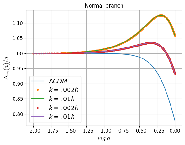
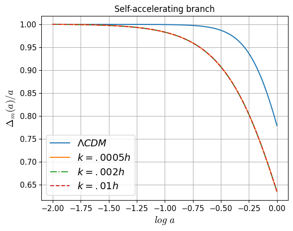
Figure 2: Left side: a) Evolution of the growth factor for the normal branch using the values obtained for the background parameters shown in Table 2: $\Omega_{m0}=0.546$, $H_{0}=69.58$ Km s^-1 Mpc^-1 and $\Omega_{r0}=0.155$ for $k=0.002h$ (orange) and $k=0.01h$ (green). b) Evolution of the growth factor for the normal branch using the values obtained for the background parameters shown in Table 3: $\Omega_{m0}=0.470$, $H_{0}=69.94$ Km s^-1 Mpc^-1 and $\Omega_{r0}=0.029$ for $k=.002h$ (red) and $k=.01h$ (purple). Right side: Evolution of the growth factor for the self-accelerating branch using the values obtained for the background parameters shown in Table 4, $\Omega_{m0}=0.286$, $H_{0}=69.08$ Km s^-1 Mpc^-1 for $k=0.0005h$ (red), $k=0.002h$ (green) and $k=0.01h$ (red). We also show the evolution of the growth factor in the $\Lambda$CDM model with the parameters values inferred from Planck $\Omega_{m0}=0.315$ and $H_{0}=67.4$ Km s^-1 Mpc^-1.

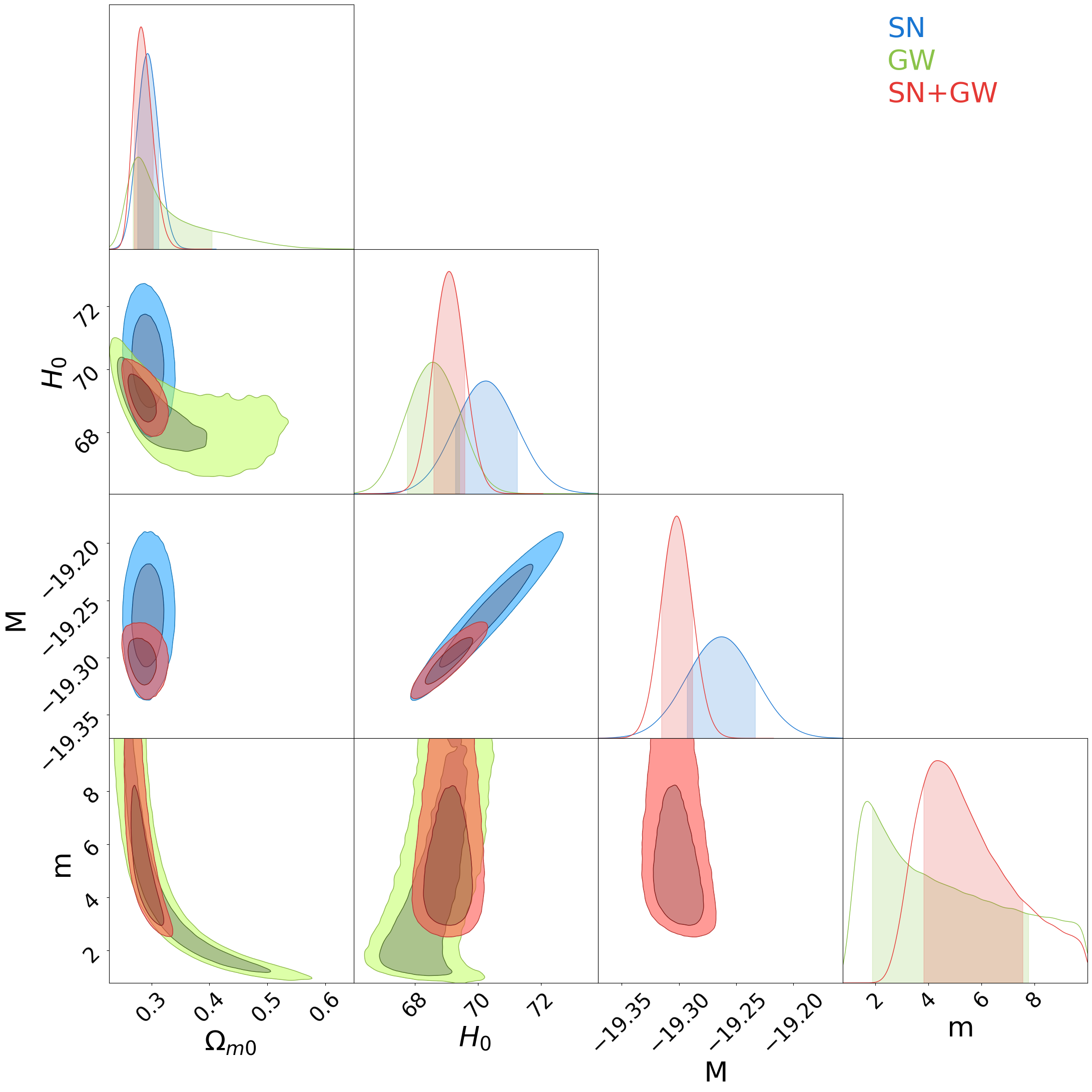
Figure 3: $2\sigma$ C.L. constraints for the background parameters using standard sirens mock data GW (green) and SN Pantheon+ (blue), and the total sample GW+Pantheon+ (red) for the normal branch using the priors shown in Table 4.

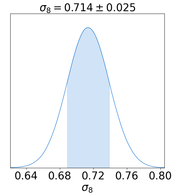
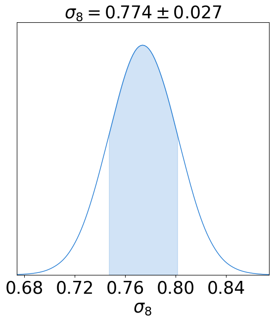
Figure 4: Left side: Posterior of $\sigma_{8}$ for the normal branch using data of Pantheon + and a flat prior for $0<\Omega_{r0}<0.25$. Right side: Posterior of $\sigma_{8}$ for the normal branch using a flat prior for $0<\Omega_{r0}<0.05$. We use a uniform prior for $\sigma_{8}\epsilon(0,1)$.

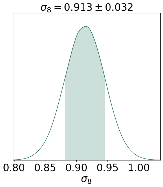
Figure 5: Posterior of $\sigma_{8}$ for the self-accelerating branch using for the background the best-fit values shown in Table 4: $\Omega_{m0}=0.286$, $H_{0}=69.08$ Km s^-1 Mpc^-1. We use a uniform prior for $\sigma_{8}\epsilon(0,1.2)$.

Parameter	Normal branch	Self-accelerating branch	$\Lambda$CDM Planck	$\Lambda$CDM SH0ES	$\Lambda$CDM Kids-1000
$\Omega_{m0}$	$0.470\pm 0.028$	$0.286\pm 0.016$	$0.315\pm 0.0007$	$0.334\pm 0.018$	$-$
$H_{0}$ [Km s-1 Mpc-1]	$69.94\pm 0.57$	$69.08\pm 0.49$	$73.6\pm 1.1$	$-$	$-$
$\sigma_{8}$	$0.774\pm 0.027$	$0.913\pm 0.032$	$0.811\pm 0.0006$	$-$	$0.76^{+0.021}_{-0.023}$

Table 5: Comparison for the values of the main cosmological parameters.

5 Conclusions

In order to constrain the value of $\sigma_{8}$, we first constrain the model parameters for the background; this is very important because it represents an update since we use the Pantheon+ catalog, which has more supernovae events than its predecessor, and furthermore, this catalog allows to constrain $H_{0}$ and $M$ independently. And as far as we know, this has not been done previously for any of these models.
For the normal branch we use two different priors for $\Omega_{r0}$. The first prior gives rise to a value of $\Omega_{m0}=0.546\pm 0.039$ for the sum of data. While for the second uniform prior $\Omega_{r0}\epsilon(0,0.05)$, we obtain $\Omega_{m0}=0.470\pm 0.028$, $H_{0}=(69.94\pm 0.57)$Km s^-1 Mpc^-1, $\Omega_{r0}=0.029$, $M=-19.281\pm 0.018$, $m=1.57\pm 0.32$ using data from the Pantheon+ catalog and the mock GW catalog. Then, we conclude that the value of $\Omega_{r0}$ has to be small in order to obtain a lower value of $\Omega_{m0}$, however $\Omega_{m0}$ is greater than the value obtained in the $\Lambda$CDM model. With the background values shown in Table 2 and Table 3 we plot the growth rate $\Delta_{m}/a$ with respect to $\log a$ in Figure 2 (left side) and we confirm the evolution of density perturbations found in previous works [1], furthermore it can be seen that the evolution of the growth rate deviates from the $\Lambda$CDM model and for a greater value of $\Omega_{m0}$ a greater deviation from the $\Lambda$CDM model.
Then in Section 2 we set the equations for the perturbations of matter density and assuming the scaling solution with $p=4$ we obtain a second order partial differential equation for $\Delta_{m}$ (26), then we use the best fit values found for $\Omega_{m0}$ and $H_{0}$ that are shown in Table 2 and Table 3, for the sum of the data, to solve it with $k=(h/8)$Mpc^-1 and then to constrain $\sigma_{8}$ we perform the statistical analysis described in Section 3.3. We found that $\sigma_{8}=0.714\pm 0.025$ when $\Omega_{m0}=0.546\pm 0.039$ and $H_{0}=(69.58\pm 0.53)$ km s^-1 Mpc^-1 and $\sigma_{8}=0.774\pm 0.027$ when $\Omega_{m0}=0.470\pm 0.028$ and $H_{0}=(69.94\pm 0.57)$ km s^-1 Mpc^-1, for the normal branch.
For the self-accelerating branch the best-fit values for the background parameters using the sum of data are: $\Omega_{m0}=0.286\pm 0.016$, $H_{0}=(69.08\pm 0.49)$ Km s^-1 Mpc^-1, $M=-19.302\pm 0.014$, $m=5.7\pm 1.7$; and the value found for $\sigma_{8}=0.913\pm 0.032$.
However, in the $\Lambda$CDM model with flat spatial curvature $\Omega_{k}=0$ using data from Pantheon+ and SH0ES, $\Omega_{m0}=0.334\pm 0.018$ and $H_{0}=(73.6\pm 1.1)$ Km s^-1 Mpc^-1 [17], while data from Planck indicate that $\Omega_{m0}=0.315\pm 0.0007$, $H_{0}=(67.4\pm 0.5)$ Km s^-1 Mpc^-1 assuming a $\Lambda$CDM cosmology [6]. Therefore the value of $\Omega_{m0}$ for the normal branch is greater than the value of matter density parameter in the $\Lambda$CDM model while the value of $\Omega_{m0}$ for the self-accelerating branch is lower. And in both models the value of $H_{0}$ is between the value found by CMB and the value found from SH0ES for the $\Lambda$CDM model. We found that the value of $\sigma_{8}$ for the normal and the self-accelerating branch differs from the value found by observations of the Cosmic Microwave Background (CMB) by Planck for the $\Lambda$CDM model which is $\sigma_{8}=0.811\pm 0.006$ [6].
On the other hand observations of large scale structures [5] have obtained a value of $\sigma_{8}=0.76^{+0.021}_{-0.023}$, this could tell us that the normal branch agree with observations of large scale structures and is a better model than the self-accelerating branch whose value of $\sigma_{8}$ is very different for the values found either by close or distant observations.
Finally we present these results in Table 5 when we compare the values found for the self-accelerating and normal branch with the $\Lambda$CDM model.

Appendix A Appendix

In [14] it was shown that the scalar perturbations are related to $\Omega$ as:

$${A}=-\frac{1}{6b}\left[2\Omega^{\prime\prime}-\frac{n^{\prime}}{n}\Omega^{\prime}+\frac{\Lambda_{5}}{6}\Omega+\frac{1}{n^{2}}\left(\ddot{\Omega}-\frac{\dot{n}}{n}\dot{\Omega}\right)\right],$$

$${A_{y}}=\frac{1}{nb}\left(\dot{\Omega}^{\prime}-\frac{n^{\prime}}{n}\dot{\Omega}\right),$$

$$\mathcal{R}=\frac{1}{6b}\left(\Omega^{\prime\prime}-\frac{1}{n^{2}}\ddot{\Omega}+\frac{\Lambda_{5}}{3}\Omega+\frac{\dot{n}}{n^{3}}\dot{\Omega}+\frac{n^{\prime}}{n}\Omega^{\prime}\right).$$ (49)

From the master equation (7) we can obtain $\Omega^{\prime\prime}$

$$\Omega^{\prime\prime}=\frac{\ddot{\Omega}}{n^{2}}-\frac{1}{n^{2}}\left(\frac{\dot{n}}{n}+3\frac{\dot{b}}{b}\right)\dot{\Omega}+\left(3\frac{b^{\prime}}{b}-\frac{n^{\prime}}{n}\right)\Omega^{\prime}+\left(\frac{\Lambda_{5}}{6}+\frac{k^{2}}{b^{2}}\right)\Omega$$ (50)

and if we replace $\Omega^{\prime\prime}$ in the set of equations (A) and evaluating $n$ and $b$ on the brane, we obtain:

$${A} = \frac{1}{6a}\left[-3\ddot{\Omega}_{b}+6H\dot{\Omega}_{b}+3\epsilon\Omega^{\prime}_{b}\left(\frac{\dot{H}}{H}-H\right)-\left(\frac{2k^{2}}{a^{2}}+\frac{\Lambda_{5}}{2}\right)\Omega_{b}\right],$$

$$\mathcal{R} = \frac{1}{6a}\left[3\epsilon H\Omega^{\prime}_{b}-3H\dot{\Omega}_{b}+\left(\frac{\Lambda_{5}}{2}+\frac{k^{2}}{a^{2}}\right)\Omega_{b}\right].$$ (51)

where the subscript $b$ indicates that it is being evaluated on the brane at $y=0$, and in this work we consider $\Lambda_{5}=0$.
In the $5D$ longitudinal gauge, the location of the brane is perturbed and given by

$$y=\xi=-r_{c}(\Phi+\Psi),$$ (52)

and the induced metric perturbations on the brane are

$$\Psi = A-\epsilon\left(\frac{\dot{H}}{H}+H\right)\xi,\hskip 14.22636pt\Phi=\mathcal{R}-\epsilon H\xi,$$ (53)

from (52) and (53) it can be found that:

$$\Phi = \frac{1}{1-r_{c}\epsilon(\dot{H}/H+2H)}\left[R\left\{1-\epsilon r_{c}\left(\frac{\dot{H}}{H}+H\right)\right\}+\epsilon Hr_{c}A\right],$$ (54)

$$\Psi = \frac{1}{1-r_{c}\epsilon(\dot{H}/H+2H)}\left[(1-\epsilon Hr_{c})A+r_{c}\epsilon\mathcal{R}\left(\frac{\dot{H}}{H}+H\right)\right],$$ (55)

then using (A) and the boundary condition (17) we can rewrite $\Phi$ and $\Psi$ in terms of $\Omega_{b}$ given by (18).

Appendix B Scaling solution

We assume a scaling solution [11] for $\Omega$ given by

$$\Omega(a,x)=\mathcal{A}a^{p}G(x)$$ (56)

such that $\Omega|_{y=0}=\mathcal{A}a^{p}$, with $x\equiv yH$, and $G|{y=0}=1$.
The causal horizon of the propagation of perturbations through bulk is given by

$$\xi=aH^{2}\int_{0}^{a}\frac{da^{\prime}}{a^{\prime 2}H(a^{\prime})^{2}}$$ (57)

then $G(x=\xi)=0.$
With this we can obtain:

$$\dot{\Omega} = \mathcal{A}a^{p}H(pG+xh\frac{dG}{dx})$$

$$\ddot{\Omega} = H^{2}\mathcal{A}a^{p}\left[(h^{2}+hp)G+(2pxh+2xh^{2}+x\tilde{h})\frac{dG}{dx}+x^{2}h^{2}\frac{d^{2}G}{dx^{2}}\right],$$ (58)

where $h=(dH/d\ln a)/H=\frac{a}{H}\frac{dH}{da}$ and $\tilde{h}=\frac{dh}{d\ln a}$.
And evaluating at $y=0$ it can be found that:

$$\Omega|_{y=0} = \mathcal{A}a^{p}$$

$$\dot{\Omega}|_{y=0} = \mathcal{A}pa^{p}H$$

$$\ddot{\Omega}|_{y=0} = H^{2}\mathcal{A}a^{p}(h^{2}+hp)=\mathcal{A}H^{2}a^{p}\left[\frac{a^{2}}{H^{2}}\left(\frac{dH}{da}\right)^{2}+\frac{p}{H}\frac{dH}{da}\right].$$ (59)

Then replacing (B) in (7) and using (2) we can find a differential equation for $G(x)$ for the normal branch given by:

$$A(x)\frac{d^{2}G}{dx^{2}}+B(x)\frac{dG}{dx}+C(x)G=0,$$ (60)

where

$$A(x) = (1-x)(1-x-2hx),$$

$$B(x) = -2x(hp+1)+2-h+\frac{(x^{2}-x)(h^{2}+h^{\prime}+h)}{1-x(h+1)},$$

$$C(x) = -p^{2}-hp-\frac{xp(h^{\prime}+h^{2}+h)}{1-x(h+1)}+\frac{3p(1-x-xh)}{1-x}-\frac{[1-x(1+h)]^{2}}{(1-x)^{2}}\frac{k^{2}}{a^{2}H^{2}},$$ (61)

that is a simplified equation of the version found in [11]. While for the accelerated branch is:

$$A(x) = (1+x)(1+x(1+2h)),$$

$$B(x) = -2x(hp+1)-2+h-\frac{(x^{2}+x)(h^{2}+h^{\prime}+h)}{1+x(h+1)},$$

$$C(x) = -p^{2}-hp+\frac{xp(h^{\prime}+h^{2}+h)}{1+x(h+1)}+\frac{3p(1+x+xh)}{1+x}-\frac{[1+x(h+1)]^{2}}{(1+x)^{2}}\frac{k^{2}}{a^{2}H^{2}},$$ (62)

and this is equivalent to the equation found in [10].
And according to [1] it can be found a boundary condition for $\Omega$ at $y=0$ which is:

$$(\partial_{y}\Omega)_{b}=-\frac{\epsilon\gamma_{1}}{2H}\ddot{\Omega}_{b}+\frac{9\epsilon\gamma_{3}}{4}\dot{\Omega}_{b}-\left(\frac{3\epsilon\gamma_{3}k^{2}}{4Ha^{2}}+\frac{H\gamma_{4}}{4}\right)\Omega_{b}+\frac{3\epsilon r_{c}\kappa_{4}^{2}\rho a^{3}\gamma_{4}}{2k^{2}}\triangle,$$ (63)

where $\gamma_{1},\gamma_{2},\gamma_{3},\gamma_{4}$ are given by:

$$\gamma_{1} = \frac{2\epsilon Hr_{c}}{2\epsilon Hr_{c}-1}=\frac{\epsilon H}{\epsilon H-H_{0}\sqrt{\Omega_{r0}}},$$

$$\gamma_{2} = \frac{2\epsilon r_{c}(\dot{H}-H^{2}+2\epsilon H^{3}r_{c})}{H(2\epsilon Hr_{c}-1)^{2}}=\frac{\epsilon H_{0}\sqrt{\Omega_{r0}}\left(a\frac{dH}{da}-H\right)+H^{2}}{(\epsilon H-H_{0}\sqrt{\Omega_{r0}})^{2}},$$

$$\gamma_{3} = \frac{4\epsilon r_{c}(2\epsilon r_{c}\dot{H}-3H+6\epsilon H^{2}r_{c})}{9(2\epsilon Hr_{c}-1)^{2}}=\frac{2aH\frac{dH}{da}+6H^{2}-6H\epsilon H_{0}\sqrt{\Omega_{r0}}}{9(\epsilon H-H_{0}\sqrt{\Omega_{r0}})^{2}},$$

$$\gamma_{4} = \frac{4\epsilon(\epsilon r_{c}\dot{H}-H+2\epsilon H^{2}r_{c})}{3H(2\epsilon Hr_{c}-1)^{2}}=\frac{H_{0}\sqrt{\Omega_{r0}}}{(\epsilon H-H_{0}\sqrt{\Omega_{r0})^{2}}}\left(\frac{2}{3}a\frac{dH}{da}-\frac{4}{3}H_{0}\sqrt{\Omega_{r0}}\epsilon+\frac{4}{3}H\right).$$ (64)

Then if we consider $\Omega=\mathcal{A}a^{p}G$ and using (B), then the boundary condition (17) can be rewritten as:

$$\frac{dG}{dx}|_{y=0}=-\frac{\epsilon\gamma 1}{2}(h^{2}+hp)+\frac{9\epsilon\gamma_{3}}{4}p-\frac{3\epsilon\gamma_{3}k^{2}}{4H^{2}a^{2}}-\frac{H\gamma_{4}}{4}+\frac{3\epsilon r_{c}\kappa_{4}^{2}\rho a^{3}\gamma_{4}}{2k^{2}}\frac{\triangle}{\mathcal{A}a^{p}H},$$ (65)

where we have used $\Omega_{b}=\mathcal{A}a^{p}G(x=0)=\mathcal{A}a^{p}$.

References

- [1] Antonio Cardoso, Kazuya Koyama, Sanjeev S. Seahra and Fabio P. Silva “Cosmological perturbations in the DGP braneworld: Numeric solution” In Phys. Rev. D 77 American Physical Society, 2008, pp. 083512 DOI: 10.1103/PhysRevD.77.083512
- [2] Eleonora Di Valentino et al. “In the realm of the Hubble tension—a review of solutions” In Classical and Quantum Gravity 38.15 IOP Publishing, 2021, pp. 153001
- [3] Elcio Abdalla et al. “Cosmology intertwined: A review of the particle physics, astrophysics, and cosmology associated with the cosmological tensions and anomalies” In Journal of High Energy Astrophysics 34, 2022, pp. 49–211 DOI: 10.1016/j.jheap.2022.04.002
- [4] Edward Macaulay, Ingunn Kathrine Wehus and Hans Kristian Eriksen “Lower Growth Rate from Recent Redshift Space Distortion Measurements than Expected from Planck” In Physical review letters 111.16 APS, 2013, pp. 161301
- [5] Catherine Heymans et al. “KiDS-1000 Cosmology: Multi-probe weak gravitational lensing and spectroscopic galaxy clustering constraints” In Astronomy & Astrophysics 646 EDP Sciences, 2021, pp. A140
- [6] Nabila Aghanim et al. “Planck 2018 results-VI. Cosmological parameters” In Astronomy & Astrophysics 641 EDP sciences, 2020, pp. A6
- [7] A Pezzotta et al. “The VIMOS Public Extragalactic Redshift Survey (VIPERS)-The growth of structure at from redshift-space distortions in the clustering of the PDR-2 final sample” In Astronomy & Astrophysics 604 EDP Sciences, 2017, pp. A33
- [8] Shinji Mukohyama “Gauge-invariant gravitational perturbations of maximally symmetric spacetimes” In Phys. Rev. D 62 American Physical Society, 2000, pp. 084015 DOI: 10.1103/PhysRevD.62.084015
- [9] Kazuya Koyama and Roy Maartens “Structure formation in the Dvali-Gabadadze-Porrati cosmological model” In Journal of Cosmology and Astroparticle Physics 2006.01 IOP Publishing, 2006, pp. 016
- [10] Ignacy Sawicki, Yong-Seon Song and Wayne Hu “Near-horizon solution for Dvali-Gabadadze-Porrati perturbations” In Physical Review D 75.6 APS, 2007, pp. 064002
- [11] Yong-Seon Song “Large scale structure formation of the normal branch in the DGP brane world model” In Phys. Rev. D 77 American Physical Society, 2008, pp. 124031 DOI: 10.1103/PhysRevD.77.124031
- [12] Dan Scolnic et al. “The Pantheon+ Analysis: Cosmological Constraints” In The Astrophysical Journal 938.2 The American Astronomical Society, 2022, pp. 110 DOI: 10.3847/1538-4357/ac8e04
- [13] Cedric Deffayet “Cosmology on a brane in Minkowski bulk” In Physics Letters B 502.1-4 Elsevier, 2001, pp. 199–208
- [14] Cédric Deffayet “On brane world cosmological perturbations” In prd 66.10, 2002, pp. 103504 DOI: 10.1103/PhysRevD.66.103504
- [15] Kei-ichi Maeda, Shuntaro Mizuno and Takashi Torii “Effective gravitational equations on a brane world with induced gravity” In Physical Review D 68.2 APS, 2003, pp. 024033
- [16] Dan Scolnic et al. “The Pantheon+ Analysis: The Full Data Set and Light-curve Release” In The Astrophysical Journal 938.2 The American Astronomical Society, 2022, pp. 113 DOI: 10.3847/1538-4357/ac8b7a
- [17] Dillon Brout et al. “The Pantheon+ analysis: cosmological constraints” In The Astrophysical Journal 938.2 IOP Publishing, 2022, pp. 110
- [18] Adam G. Riess et al. “A Comprehensive Measurement of the Local Value of the Hubble Constant with 1 km s-1 Mpc-1 Uncertainty from the Hubble Space Telescope and the SH0ES Team” In The Astrophysical Journal Letters 934, 2021 URL: https://api.semanticscholar.org/CorpusID:245005861
- [19] Maxence Corman et al. “Constraining cosmological extra dimensions with gravitational wave standard sirens: From theory to current and future multimessenger observations” In Phys. Rev. D 105.6, 2022, pp. 064061 DOI: 10.1103/PhysRevD.105.064061
- [20] Maxence Corman, Celia Escamilla-Rivera and M.. Hendry “Constraining extra dimensions on cosmological scales with LISA future gravitational wave siren data” In JCAP 02, 2021, pp. 005 DOI: 10.1088/1475-7516/2021/02/005
- [21] Maribel Hernández-Márquez and Celia Escamilla-Rivera “Strengthening interacting agegraphic dark energy DGP constraints with local measurements and multimessenger forecastings” In International Journal of Modern Physics D 33.07n08, 2024, pp. 2450029 DOI: 10.1142/S0218271824500299
- [22] George Alestas, Lavrentios Kazantzidis and Savvas Nesseris “Machine learning constraints on deviations from general relativity from the large scale structure of the Universe” In Physical Review D 106.10 APS, 2022, pp. 103519
- [23] Lucas Lombriser, Wayne Hu, Wenjuan Fang and Uroš Seljak “Cosmological constraints on DGP braneworld gravity with brane tension” In Physical Review D—Particles, Fields, Gravitation, and Cosmology 80.6 APS, 2009, pp. 063536
- [24] Ruth Lazkoz and Elisabetta Majerotto “Cosmological constraints combining H (z), CMB shift and SNIa observational data” In Journal of Cosmology and Astroparticle Physics 2007.07 IOP Publishing, 2007, pp. 015