On the Precise Asymptotics and Refined Regret of the Variance-Aware UCB Algorithm

Abstract

In this paper, we study the behavior of the Upper Confidence Bound-Variance (UCB-V) algorithm for Multi-Armed Bandit (MAB) problems, a variant of the canonical Upper Confidence Bound (UCB) algorithm that incorporates variance estimates into its decision-making process. More precisely, we provide an asymptotic characterization of the arm-pulling rates of UCB-V, extending recent results for the canonical UCB in Kalvit and Zeevi (2021) and Khamaru and Zhang (2024). In an interesting contrast to the canonical UCB, we show that the behavior of UCB-V can exhibit instability, meaning that the arm-pulling rates may not always be asymptotically deterministic. Besides the asymptotic characterization, we also provide non-asymptotic bounds for arm-pulling rates in the high probability regime, offering insights into regret analysis. As an application of this high probability result, we show that UCB-V can achieve a refined regret bound, previously unknown even for more complicate and advanced variance-aware online decision-making algorithms.

1 Introduction

1.1 Overview

The MAB problem is a fundamental framework that captures the exploration vs. exploitation trade-off in sequential decision-making. Over the past decades, this problem has been rigorously studied and widely applied across diverse fields, including dynamic pricing, clinical trials, and online advertising (Russo et al., 2018; Slivkins et al., 2019; Lattimore and Szepesvári, 2020).

In the classic $K$-armed MAB problem, a learner is faced with $K$ arms, each associated with an unknown reward distribution $P_{a}$ for $a\in[K]$, supported on $[0,1]$ with mean $\mu_{a}$ and variance $\sigma_{a}^{2}$. At each time step $t\in[T]$, the learner selects an arm $a_{t}$ and receives a reward $X_{t}$, independently drawn from $P_{a_{t}}$. The learner’s goal is to maximize the cumulative reward by striking an optimal balance between exploration (sampling less-known arms to improve estimates) and exploitation (selecting arms with high estimated rewards). This objective is commonly framed as a regret minimization problem, where the regret over a time horizon $T$ is defined as:

$$\mathrm{Reg}(T)\equiv\sum_{t=1}^{T}(\mu_{a^{\star}}-\mu_{a_{t}}),$$

where $a^{\star}\equiv\arg\max_{a\in[K]}\mu_{a}$ is the optimal arm with the highest expected reward.

Algorithm 1 UCB-V Algorithm

1: Input: Arm number $K,$ time horizon $T$, exploration coefficient $\rho$.

2: Pull each of the $K$ arms once in the first $K$ iterations.

3: for $t=K+1$ to $T$ do

4:  Compute the total number of times arm $a$ is pulled up to time $t$

$$n_{a,t}\equiv\sum_{s\in[t-1]}\bm{1}\{A_{s}=a\},\quad a\in[K].$$

5:  Compute the empirical mean and variances:

$$\bar{X}_{a,t}\equiv\frac{1}{n_{a,t}}\sum_{s\in[t-1]}\bm{1}\{a_{s}=a\}X_{s},\quad\widehat{\sigma}^{2}_{a,t}\equiv\frac{1}{n_{a,t}}\sum_{s\in[t-1]}\bm{1}\{a_{s}=a\}(X_{s}-\bar{X}_{a,t})^{2}.$$

6:  Compute the optimistic rewards:

$$\mathrm{UCB}(a,t)\equiv\bar{X}_{a,t}+\bigg{(}\frac{\widehat{\sigma}_{a,t}}{\sqrt{\rho\log T}}\vee\frac{1}{\sqrt{n_{a,t}}}\bigg{)}\cdot\frac{\rho\log T}{\sqrt{n_{a,t}}},\quad a\in[K].$$

7:  Choose arm $A_{t}$ given by:

$$A_{t}=\arg\max_{a\in[K]}\mathrm{UCB}(a,t).$$

8: end for

The minimax-optimal regret for the $K$-armed bandit problems is known to be $\Theta(\sqrt{KT})$ up to logarithmic factors. This rate is achievable by several well-established algorithms, including the UCB (Auer, 2002; Audibert et al., 2009), Thompson Sampling (Agrawal and Goyal, 2012; Russo et al., 2018), and Successive Elimination (Even-Dar et al., 2006), among others. Beyond regret minimization, increasing attention has been devoted to analyzing finer properties and the large $T$ behaviours of several typical algorithms, including the regret tail distributions (Fan and Glynn, 2021b, 2022), diffusion approximations (Fan and Glynn, 2021a; Kalvit and Zeevi, 2021; Araman and Caldentey, 2022; Kuang and Wager, 2023), arm-pulling rates (Kalvit and Zeevi, 2021; Khamaru and Zhang, 2024). Among these works, Kalvit and Zeevi (2021) and Khamaru and Zhang (2024) introduced the concept of stability for the canonical UCB algorithm, enabling the precise characterization of arm-pulling behaviors and facilitating statistical inference for adaptively collected data, a task traditionally considered challenging for general bandit algorithms.

In more structured settings, sharper regret bounds are achievable, particularly when arm variances are small. For instance, if all arms have zero variance (i.e., deterministic rewards), a single pull of each arm is sufficient to identify the optimal one. This observation has motivated an active research area on developing variance-aware algorithms for bandit problems (Auer, 2002; Audibert et al., 2007, 2009; Honda and Takemura, 2014; Mukherjee et al., 2018; Zhang et al., 2021; Zhao et al., 2023; Saha and Kveton, 2024). Among them, the UCB-V algorithm (Audibert et al., 2007, 2009), detailed in Algorithm 1, adapts the classic UCB algorithm by incorporating variance estimates of each arm.

While regret minimization for variance-aware algorithms has been well-studied, their precise arm-pulling behavior remains less explored. The main challenge here is that utilizing variance information introduces a new quantity, in addition to $\Delta$, that influences the arm-pulling rates. Actually, the behavior of the algorithm can differ significantly depending on whether variance information is incorporated or not. In Figures 1 and 2(b), we compare the empirical arm-pulling rates between UCB-V and canonical UCB in a two-armed setting. Compared to canonical UCB, its variance-aware version exhibits significantly greater fluctuations in arm-pulling numbers as $\Delta$ changes, and its arm-pulling distribution is more heavy-tailed. This highlights the significant differences in the variance-aware setting and introduces additional challenges.

In this work, we try to close this gap by presenting an asymptotic analysis of UCB-V. As in Kalvit and Zeevi (2021) and Khamaru and Zhang (2024), our main focus is on the arm-pulling numbers and stability. For clarity, we concentrate on the two-armed bandit setting, specifically $K=2$, in the main part of our paper, as it effectively captures the core exploration-exploitation trade-off while allowing a precise exposition of results (Rigollet and Zeevi, 2010; Goldenshluger and Zeevi, 2013; Kaufmann et al., 2016; Kalvit and Zeevi, 2021). The extension to the $K$-armed case is discussed in Section 5.

More precisely, by providing a general concentration result, we establish both precise asymptotic characterizations and high-probability bounds of the arm-pulling numbers of UCB-V. When $\sigma_{1},\sigma_{2}=\Omega(1)$ our results provide a straightforward generalization of those for canonical UCB. In contrast, when $\sigma_{1}\ll\sigma_{2}$, we show that, unlike UCB, the stability result may not holds for UCB-V and reveals a phase transition phenomenon of the optimal arm pulling numbers, as illustrated in Figure 2. Finally, as an application of our sharp characterization of arm-pulling rates, we present a refined regret result for UCB-V, a result previously unknown for any other variance-aware decision-making algorithms. We summarize our contributions in more detail below. For simplicity of notation, we assume the optimal arm $a^{\star}=1$ and denote $\Delta=\Delta_{2}.$

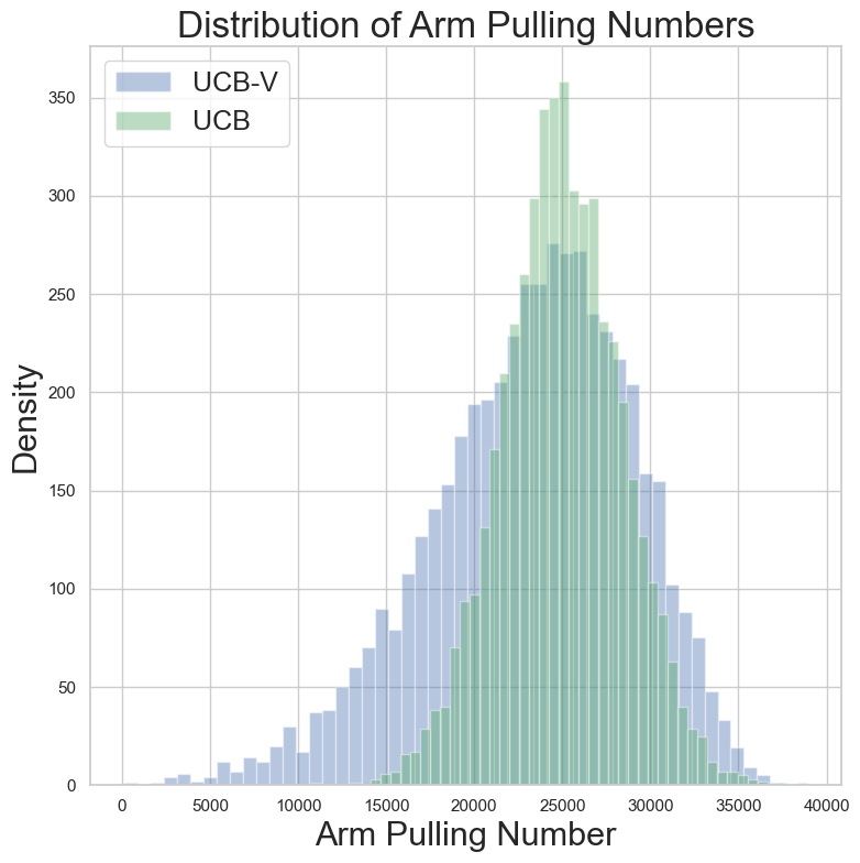
(a) $\sigma_{1}=\sigma_{2}=1/4,\Delta=0$

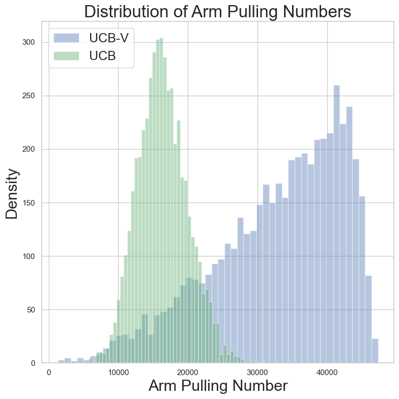
(b) $\sigma_{1}=0,\sigma_{2}=1/4,\Delta=\sigma_{2}\sqrt{\log T/T}$

Figure 1: Arm-pulling times of UCB-V and UCB for different variance parameters, both with $T=50,000$ and $5000$ repetitions.

Precise asymptotic behaviour for UCB-V

For fixed values of $\Delta,\sigma_{1},\sigma_{2},T$, we propose deterministic equations with a unique solution, $\{n_{a,T}^{\star}\}_{a=1,2}$, and demonstrate that the UCB-V arm-pulling numbers $n_{1,T}$ and $n_{2,T}$ are asymptotically equivalent to $n_{1,T}^{\star}$ and $n_{2,T}^{\star}$, except when $\sigma_{1}\ll\sigma_{2}$ and $\sigma_{2}\sqrt{\rho\log T}/(\sqrt{T}\Delta)=1$ simultaneously hold. This phenomenon, referred to as the stability of arm-pulling numbers, is formally defined in Definition 4. Consequently, the solutions of these deterministic equations can be used to predict the behavior of UCB-V in the large $T$ regime, as illustrated in Figure 2. Our results reveal several notable differences between UCB-V and the canonical UCB, as analyzed in Kalvit and Zeevi (2021) and Khamaru and Zhang (2024), due to the incorporation of variance information:

• When $\sigma_{1},\sigma_{2}=\Omega(1)$, the optimal arm will always be pulled for linear times, with $n_{1,T}\asymp\frac{\sigma_{1}^{2}}{\sigma_{1}^{2}+\sigma_{2}^{2}}T$ as $\Delta\to 0$. This indicates that in the small gap regime, the UCB-V algorithm tends to allocate more pulling times to the arm with higher reward variance, this generalizes the result for canonical UCB, where both arms are pulled for $T/2$ times in the small $\Delta$ regime.

• When $\sigma_{1}=\mathfrak{o}(\sigma_{2})$, UCB-V may pull the optimal arm sub-linearly in the small $\Delta$ regime. In contrast, the canonical UCB pulls the optimal arm linearly in $T$, as illustrated in Figure 2(b). This behavior is governed by the ratio $\Lambda_{T}\equiv\sigma_{2}\sqrt{\rho\log T}/(\sqrt{T}\Delta)$. More precisely,

  1. When $\operatorname*{\overline{lim}}_{T\to\infty}\Lambda_{T}<1$, we have $n_{a^{\star},T}/n_{T}^{\star}\xrightarrow{p}1$ for some deterministic sequence $\{n_{T}^{\star}\}_{T=1}^{\infty}$ with $n_{T}^{\star}=\Omega(T)$.

  2. When $\operatorname*{\underline{lim}}_{T\to\infty}\Lambda_{T}>1$, we have $n_{a^{\star},T}/n_{T}^{\star}\xrightarrow{p}1$ for some deterministic sequence $\{n_{T}^{\star}\}_{T=1}^{\infty}$ with $n_{T}^{\star}=\mathcal{O}(\sqrt{T}/\sigma_{2})$

  3. When $\lim_{T\to\infty}\Lambda_{T}=1,$ we have there exists some bandit instance so that for sufficiently large $T$, it holds

     $$\operatorname{\mathbb{P}}\Big{(}n_{1,T}\gtrsim T\Big{)}\wedge\operatorname{\mathbb{P}}\Big{(}n_{1,T}\lesssim\sqrt{T}/\sigma_{2}\Big{)}\gtrsim 1.$$

  The above results completely characterize the behavior of $n_{1,T}$ in the $\sigma_{1}=\mathfrak{o}(\sigma_{2})$ regime. Notably, we establish a phase transition in the optimal-armed pulling times $n_{1,T}$, shifting from $\mathcal{O}(\sqrt{T}/\sigma_{2})$ to $\Omega(T)$ at the critical point $\Lambda_{T}=1$. We also note that the existence of an unstable instance when $\Lambda_{T}\sim 1$ highlights a stark contrast between UCB-V and the canonical UCB, where it has been shown that the behavior of $n_{1,T}$ for any $\Delta>0$ can be asymptotically described by a deterministic sequence $\{n_{T}^{\star}\}$ as $T\to\infty$.

High probability bounds and confidence region for arm pulling numbers

While our asymptotic theory provides the precise limiting behavior of UCB-V, it has a drawback similar to those in Kalvit and Zeevi (2021) and Khamaru and Zhang (2024): the convergence rate in probability is quite slow. Specifically, the probability that the uncontrolled event occurs decays at a rate of $\mathcal{O}(1/\log T)$. This slow rate is inadequate to offer insight or guarantees in the popular high probability regime for studying bandit algorithms, where the probability of an uncontrolled event should be on the order of $\mathcal{O}(1/T)$. To address this gap, we demonstrate that, starting from our unified concentration result in Proposition 1, one can derive non-asymptotic bounds for arm pulling numbers in the high probability regime. This result provides a high probability confidence region for arm pulling numbers, as illustrated in the Figure 3(a).

Refined regret for variance-aware decision making

As an application of our high probability arm-pulling bounds, we demonstrate in Section 4 that the UCB-V algorithm achieves a refined regret bound of the form

$$\mathcal{O}\bigg{(}\frac{\sigma_{2}^{2}}{\sigma_{1}\vee\sigma_{2}}\sqrt{T}\bigg{)}.$$

This result improves upon the best-known regret for UCB-V (Audibert et al., 2009; Talebi and Maillard, 2018) and surpasses the regrets for all known variance-aware bandit algorithms (Zhao et al., 2023; Zhang et al., 2021; Saha and Kveton, 2024; Dai et al., 2022; Di et al., 2023), which are of the form $\mathcal{O}(\sigma_{2}\sqrt{T})$ in the two-armed setting. Our result is the first to reveal the effect of the optimal arm’s variance: When $\sigma_{1}=\mathfrak{o}(\sigma_{2})$, the regret matches the previous known $\mathcal{O}(\sigma_{2}\sqrt{T})$ bound, and the optimal arm’s variance doesn’t affect performance; as $\sigma_{1}$ surpasses $\sigma_{2}$, the regret decreases as $\sigma_{1}$ increases, following the form $\mathcal{O}(\frac{\sigma_{2}^{2}}{\sigma_{1}}\sqrt{T})$. Simulations presented in Figure 2 confirm our predictions, demonstrating that UCB-V exhibits improved performance in high $\sigma_{1}$ scenarios, which was previously unknown.

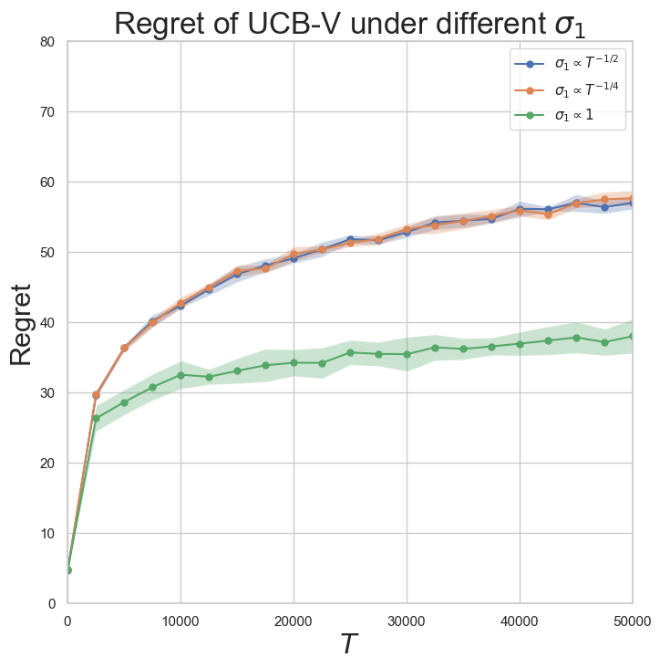
(a) Regrets of UCB-V under different $\sigma_{1}$

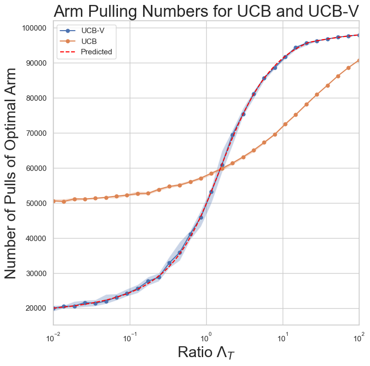
(b) Arm Pulling Numbers

Figure 2: (a): Regret of UCB-V with $\sigma_{2}\asymp T^{-1/4},\Delta\asymp 1/\sqrt{T}$ fixed and $\sigma_{1}\asymp T^{-1/2},T^{-1/4},1$, each instance with 10 repetitions. (b): The median and 30% quantile of optimal arm pulling times, $n_{1,T}$, for UCB and UCB-V, under varying $\Lambda_{T}$ in the $\sigma_{1}=\mathfrak{o}(\sigma_{2})$ regime, with $T=1,000,000$ over 30 repetitions for each $\Delta$. The red dotted line is the predicted $n_{1,T}$ of UCB-V using (6).

1.2 Related Works

Variance-aware decision making

In the multi-armed bandit setting, leveraging variance information to balance the exploration-exploitation trade-off was first studied by Auer (2002) and Audibert et al. (2007, 2009), where the UCB-V algorithm was proposed and analyzed. Beyond the optimistic approach, (Mukherjee et al., 2018) examined elimination-based algorithms that utilize variance information, while Honda and Takemura (2014) and Saha and Kveton (2024) focused on analyzing the performance of Thompson sampling in variance-aware contexts.

Beyond the MAB model, variance information has been utilized in contextual bandit and Markov Decision Process settings (Talebi and Maillard, 2018; Zhang et al., 2021; Dai et al., 2022; Zhao et al., 2023; Di et al., 2023; Xu et al., 2024). Among these works, Zhang et al. (2021) and Zhao et al. (2023) are most relevant to our study for linear contextual bandits. especially regarding linear contextual bandits. Although they consider a different model for variance, their algorithms can be adapted to our setting, providing a $(\sigma_{1}\vee\sigma_{2})\sqrt{T}$ regret guarantee. We elaborate on this discussion in Section 4.

Asymptotic behaviours analysis in multi-armed bandits

Our investigation into the asymptotic behaviors of UCB-V is inspired by recent advancements in the precise characterization of arm-pulling behavior (Kalvit and Zeevi, 2021; Khamaru and Zhang, 2024), which focused on the canonical UCB algorithm. Beyond canonical UCB algorithm, another line of research explores the asymptotic properties of bandit algorithms within Bayesian frameworks, particularly under diffusion scaling (Fan and Glynn, 2021a; Araman and Caldentey, 2022; Kuang and Wager, 2023), where reward gaps scale as $1/\sqrt{T}$. Additionally, a noteworthy body of work Fan and Glynn (2021b, 2022); Simchi-Levi et al. (2023) conducts asymptotic analyses in the regime as in Lai and Robbins (1985), where the reward gaps $\Delta$ remain constant as $T$ increases.

Inference with adaptively collected data

In addition to regret minimization, there is a growing interest in statistical inference for bandit problems. A significant body of research addresses online debiasing and adaptive inference methods (Dimakopoulou et al., 2021; Chen et al., 2021, 2022; Duan et al., 2024), but our findings are more closely related to studies focused on post-policy inference (Nie et al., 2018; Zhang et al., 2020; Hadad et al., 2021; Zhan et al., 2021). These works aim to provide valid confidence intervals for reward-related quantities based on data collected from pre-specified adaptive policies. Among them, the most relevant works are Kalvit and Zeevi (2021) and Khamaru and Zhang (2024). The former addresses the inference guarantee of $Z$-estimators collected by UCB in the two-armed setting, while the latter extends this to the $K$-armed setting. In particular, these two works assert the stability of the pulling time for the optimal arm under arbitrary gap conditions $\Delta$, enabling the application of the martingale Central Limit Theorem (CLT) to obtain asymptotically normal estimator of $\mu^{\star}$. However, our results point out a critical regime where such stability breaks down, as shown in Figure 4(b), highlighting the price of utilizing variance information to enhance regret minimization performance.

1.3 Notation

For any positive integer $n$, let $[n]=[1:n]$ denote the set $\{1,\ldots,n\}$. For $a,b\in\mathbb{R}$, $a\vee b\equiv\max\{a,b\}$ and $a\wedge b\equiv\min\{a,b\}$. For any $a\in\mathbb{R}$, $a_{+}\equiv\max\{a,0\}$.

Throughout this paper, we regard $T$ as our fundamental large parameter. For any possibly $T$-dependent quantities $a\equiv a(T)$ and $b\equiv b(T)$, we say $a=\mathfrak{o}(b)$ or $b=\omega(a)$ if $\lim_{T\to\infty}a/b=0$. Similarly, $a=\mathcal{O}(b)$ or $b=\Omega(a)$ if $\lim_{T\to\infty}\lvert a/b\rvert\leq C$ for some constant $C$. If $a=\mathcal{O}(b)$ and $a=\Omega(b)$ hold simultaneously, we say $a=\Theta(b)$, or $a\asymp b$, and we write $a\sim b$ in the special case when $\lim_{T\to\infty}a/b=1$. If either sequence $a$ or $b$ is random, we say $a=\mathfrak{o}_{\mathbf{P}}(b)$ if $a/b\xrightarrow{p}0$ as $T\to\infty$.

1.4 Organization

The remainder of the paper is organized as follows. We begin by presenting implicit bounds on arm-pulling numbers in Section 2. These implicit bounds serve as motivation for our main results: the asymptotic characterization of the arm-pulling numbers for the UCB-V algorithm in Section 3, and a refined regret analysis for variance-aware decision-making in Section 4. Additionally, we extend our discussion to the $K$-arm setting in Section 5. All proofs and technical lemmas are relegated to the appendix.

2 Implicit bounds of arm-pulling numbers

2.1 Additional notation

For $\rho>1$ and $T\in\mathbb{N}_{+}$, let

$$\overline{\sigma}_{a}(\rho;T)\equiv\frac{\sigma_{a}}{\sqrt{\rho\log T}},\quad\overline{\Delta}_{a}(\rho;T)\equiv\frac{\Delta_{a}}{\rho\log T},\quad a\in[K].$$

Whenever there is no confusion, we will simply write $\overline{\sigma}_{a}\equiv\overline{\sigma}_{a}(\rho;T)$ and $\overline{\Delta}_{a}\equiv\overline{\Delta}_{a}(\rho;T)$. We shall also mention that $\sigma_{a}$ and $\Delta_{a}$ may vary with $T$.

Next, for any $\sigma\geq 0$ and $n\in\mathbb{N}_{+}$, we define

$$\varphi(n;\sigma)\equiv\frac{\sigma\vee n^{-1/2}}{\sqrt{n}}.$$

It is straightforward to verify that for each fixed $\sigma\geq 0$, the function $\varphi(\cdot;\sigma):\mathbb{R}_{\geq 0}\to\mathbb{R}_{\geq 0}$ is monotonic. Its inverse, denoted $n(\cdot;\sigma):\mathbb{R}_{\geq 0}\to\mathbb{R}_{\geq 0}$, is given by $n(\varphi;\sigma)\equiv(\sigma^{2}\vee\varphi)/\varphi^{2}$. Consequently, studying the behavior of $n_{a,T}$ corresponds to analyzing $\varphi(n_{a,T};\overline{\sigma}_{a})$. For simplicity, we denote $\varphi_{a,t}\equiv\varphi(n_{a,t};\overline{\sigma}_{a})$ for any $a\in[K]$ and $t\in[T]$.

2.2 Implicit bounds of arm-pulling numbers

Consider the Algorithm 1 with $K=2$. Our starting point is the following concentration result for $\varphi_{a,T},a\in[2]$.

Proposition 1.

Recall that $\overline{\sigma}_{a}\equiv\overline{\sigma}_{a}(\rho;T)$ and $\overline{\Delta}_{a}\equiv\overline{\Delta}_{a}(\rho;T)$ for $a\in[2]$. Fix any $\delta>0$, $\rho>1$ and any positive integer $T\geq 4$ such that

$$\varepsilon\equiv\varepsilon(\delta;\rho;T)\equiv 5\bigg{(}\sqrt{48\frac{\log(\log(T/\delta)/\delta)}{\rho\log T}}+\frac{128\log(1/\delta)}{\rho\log T}\bigg{)}^{1/2}+\frac{200}{\sqrt{T}}\leq\frac{1}{2}.$$

Then, with probability at least $1-\delta$, we have

$$\bigg{(}\frac{1-\varepsilon}{1+\varepsilon}\bigg{)}^{4}\leq\frac{\overline{\sigma}_{1}^{2}\vee\varphi_{1,T}}{T\varphi^{2}_{1,T}}+\frac{\overline{\sigma}_{2}^{2}\vee(\varphi_{1,T}+\overline{\Delta}_{2})}{T(\varphi_{1,T}+\overline{\Delta}_{2})^{2}}\leq\bigg{(}\frac{1+\varepsilon}{1-\varepsilon}\bigg{)}^{4},$$

and

$$\bigg{(}\frac{1-\varepsilon}{1+\varepsilon}\bigg{)}^{4}\leq\frac{\varphi_{2,T}}{\varphi_{1,T}+\overline{\Delta}_{2}}\leq\bigg{(}\frac{1+\varepsilon}{1-\varepsilon}\bigg{)}^{4}.$$

The proof of Proposition 1 is inspired by the delicate analysis of bonus terms for canonical UCB (Khamaru and Zhang, 2024) for large $T$ regime and leaved to Section A.1. Proposition 1 establishes a sandwich inequality, demonstrating that as the term $\varepsilon(\delta;\rho;T)$ approaches $0$, the concern ratio converges to $1$. This can be viewed as a non-asymptotic and variance-aware extension of the results found in Kalvit and Zeevi (2021) and Khamaru and Zhang (2024) for canonical UCB. To incorporate variance information, we have also developed a Bernstein-type non-asymptotic law of iterated logarithm result in Lemma 19, which is of independent interest. We would like to make several comments regarding Proposition 1:

1. Deriving the asymptotic equation. When selecting $\delta=(\log T)^{-1}$, we find that for any $\rho>0$, the $\varepsilon(\delta;\rho;T)$ term approaches $0$ at a rate of $\mathcal{O}\big{(}\frac{\log\log T}{\log T}\big{)}$. Under this selection, Proposition 1 yields the following probability convergence guarantee:

   $$\frac{\overline{\sigma}_{1}^{2}\vee\varphi_{1,T}}{T\varphi^{2}_{1,T}}+\frac{\overline{\sigma}_{2}^{2}\vee(\varphi_{1,T}+\overline{\Delta}_{2})}{T(\varphi_{1,T}+\overline{\Delta}_{2})^{2}}=1+\mathfrak{o}_{\mathbf{P}}(1).$$ (1)

   It is noteworthy that in this asymptotic result, the $\mathfrak{o}_{\mathbf{P}}(1)$ term converges to 0 at a relatively slow rate, both in probability and magnitude. For each $T$, it has a probability of at least $1-\mathcal{O}\big{(}\frac{1}{\log T}\big{)}$ to be bounded by $\mathcal{O}\big{(}\frac{\log\log T}{\log T}\big{)}$. This slow rate not only appears in our result but also in Kalvit and Zeevi (2021) and Khamaru and Zhang (2024), necessitating a considerably large $T$ to observe theoretical predictions clearly in experiments, as illustrated in Figure 2(b).

2. Permission values of $\rho$ for high probability bounds. One popular scale selection of $\delta$ is $\delta\asymp 1/T^{2},$ where (1) turns to be a high-probability guarantee that well-adopted in pure-exploration and regret analysis literature (Auer, 2002; Audibert et al., 2007). With such selection, the requirement $\varepsilon(\delta;\rho;T)<1/2$ turns to be $\rho>c^{\prime}$ for some universal and sufficiently large constant $c^{\prime}$. Thus, we have with probability at least $1-\mathcal{O}(1/T^{2})$:

   $$1-(c^{\prime})^{-1}\leq\frac{\overline{\sigma}_{1}^{2}\vee\varphi_{1,T}}{T\varphi^{2}_{1,T}}+\frac{\overline{\sigma}_{2}^{2}\vee(\varphi_{1,T}+\overline{\Delta}_{2})}{T(\varphi_{1,T}+\overline{\Delta}_{2})^{2}}\leq 1+(c^{\prime})^{-1}.$$ (2)

   In particular, since the centered term is a monotone increasing function of $\varphi_{1,T}$, this result provides a high-probability confidence region for $\varphi_{1,T}$ and consequently for $n_{1,T}$, as shown Figure 3(a). We will further apply such high probability bounds of $n_{1,T}$ to derive the refined regret bound for UCB-V in section 4.

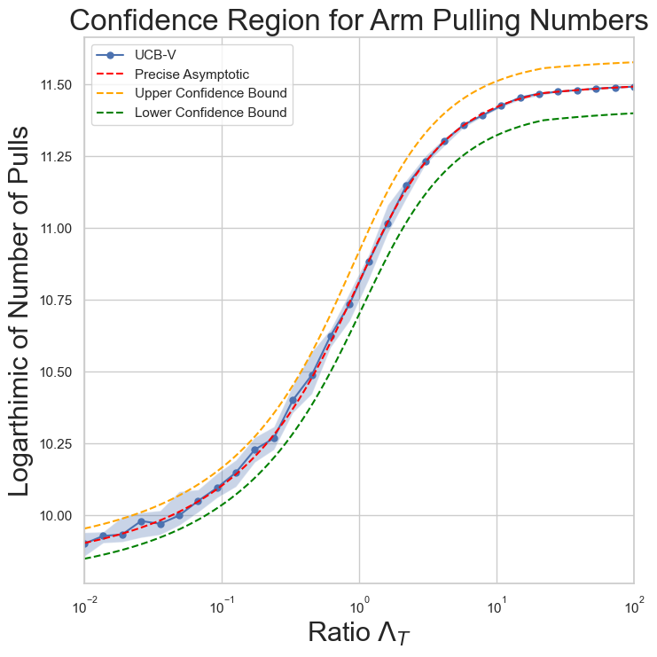
(a) Confidence region of $n_{1,T}$

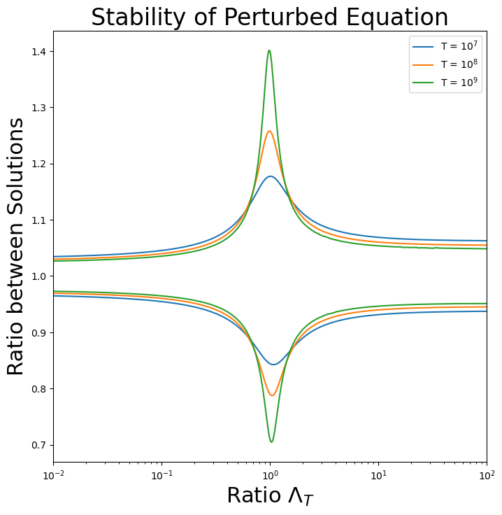
(b) Stabbility of perturbed equation

Figure 3: (a): Confidence region of arm pulling numbers under different $\Lambda_{T}$, with $\sigma_{1}=\mathfrak{o}(\sigma_{2})$. The dotted lines represent the exact and perturbed solutions of (3), where the perturbed curves solves $f(\varphi)=1\pm 1/\log T$. The UCB-V line shows the number of arm pulls under the UCB-V algorithm with 30% quantile, with $T=10^{5}$ over 30 repetitions. (b): The ratio between the perturbed solution $f(\varphi)=1\pm 1/\log T$ and the exact solution $f(\varphi)=1$ is shown for $T=10^{5};10^{7};10^{9}$ under different $\Lambda_{T}$. It can be seen that the ratio deviates from 1 as $\Lambda_{T}\to 1$ with increasing $T$.

The implications outlined above will be made precise in the subsequent two sections.

3 Asymptotic characterization of arm-pulling numbers

3.1 Stability of the asymptotic equation

Consider the deterministic equation

$$f(\varphi)=1\quad\text{with}\quad f(\varphi)\equiv\frac{\overline{\sigma}_{1}^{2}\vee\varphi}{T\varphi^{2}}+\frac{\overline{\sigma}_{2}^{2}\vee(\varphi+\overline{\Delta}_{2})}{T(\varphi+\overline{\Delta}_{2})^{2}}.$$ (3)

Recall that $\overline{\sigma}_{a}\equiv\sigma_{a}/\sqrt{\rho\log T}$ and $\overline{\Delta}_{a}\equiv\Delta_{a}/(\rho\log T)$ for $a=1,2$, so the equation actually depends on both $\rho$ and $T$. For any fixed $T\in\mathbb{N}_{+}$ and $\rho>1$, Proposition 1 indicates that $\varphi_{1,T}$ satisfies $f(\varphi_{1,T})=1+\delta$, where $\delta$ represents a perturbation term. Given the asymptotic equation derived in (1), it is reasonable to conjecture that the behavior of $\varphi_{1,T}$ aligns with the solution of the above deterministic equation. To formally connect $\varphi_{1,T}$ with the solution of (3), we conduct a perturbation analysis of this equation. Specifically, we have the following result:

Lemma 2.

Fix any $T\in\mathbb{N}_{+}$ and $\rho>1$. The following hold.

1. The fixed point equation (3) admits a unique solution $\varphi^{\star}\in(1/T,1)$.

2. Suppose that there exists some $\delta\in(-1/2,1/2)$ and $\varphi_{\delta}$ such that $f(\varphi_{\delta})=1+\delta$, we have

   $$\bigg{\lvert}\frac{\varphi_{\delta}}{\varphi^{\star}}-1\bigg{\rvert}\leq 27\lvert\delta\rvert\cdot\bigg{(}1+\bigg{\lvert}\frac{\overline{\sigma}_{2}^{2}}{T\overline{\Delta}_{2}^{2}}-1\bigg{\rvert}^{-1}\wedge\frac{\overline{\sigma}_{2}}{\overline{\sigma}_{1}\vee T^{-1/2}}\bigg{)}.$$ (4)

The proof of Lemma 2 is provided in Section B.1. Intuitively, Lemma 2 asserts that in either the homogeneous variance case ($\sigma_{2}\asymp\sigma_{1}$) or when the ratio $\overline{\sigma}_{2}^{2}/(T\overline{\Delta}_{2})^{2}$ is bounded away from 1, the solution $\varphi_{\delta}$ of the $\delta$-perturbed equation is provably bounded by $\big{(}1\pm\mathcal{O}(\delta)\big{)}\varphi^{\star}$. However, when $\sigma_{1}=\mathfrak{o}(\sigma_{2})$ and the ratio $\overline{\sigma}_{2}^{2}/(T\overline{\Delta}_{2})^{2}$ approaches 1, the stability guarantee of the lemma breaks down. Although this result may seem pessimistic—as $\overline{\sigma}_{2}^{2}/(T\overline{\Delta}_{2})^{2}\sim 1$ causes the right-hand side of (4) to diverge—it accurately reflects the behavior of the perturbed solution. This is illustrated in Figure 3(b), where instability arises when $\overline{\sigma}_{2}^{2}/(T\overline{\Delta}_{2})^{2}=1$.

3.2 Asymptotic Stability

One important corollary of the perturbation bound is the following asymptotic stability result. Recall that $\overline{\Delta}_{a}\equiv\Delta_{a}/(\rho\log T)$ and $\overline{\sigma}_{a}\equiv\sigma_{a}/\sqrt{\rho\log T}$ for $a\in[2]$.

Theorem 3.

Consider Algorithm 1 with $K=2$. Suppose that

$$\operatorname*{\overline{lim}}_{T\to\infty}\Bigg{\{}\bigg{\lvert}\frac{\overline{\sigma}_{2}^{2}}{T\overline{\Delta}_{2}^{2}}-1\bigg{\rvert}^{-1}\wedge\frac{\overline{\sigma}_{2}}{\overline{\sigma}_{1}\vee T^{-1/2}}\Bigg{\}}<\infty.$$ (5)

Then for $a\in[2]$, we have

$$\frac{n_{a,T}}{n_{a,T}^{\star}}\xrightarrow{p}1,$$

where $n_{1,T}^{\star}$ is the unique solution to the following equation:

$$\frac{\overline{\sigma}_{1}^{2}\vee\varphi(n_{1,T}^{\star};\overline{\sigma}_{1})}{T\varphi^{2}(n_{1,T}^{\star};\overline{\sigma}_{1})}+\frac{\overline{\sigma}_{2}^{2}\vee(\varphi(n_{1,T}^{\star};\overline{\sigma}_{1})+\overline{\Delta}_{2})}{T(\varphi(n_{1,T}^{\star};\overline{\sigma}_{1})+\overline{\Delta}_{2})^{2}}=1,$$ (6)

and

$$n_{2,T}^{\star}\equiv\frac{\overline{\sigma}_{2}^{2}\vee(\varphi(n_{1,T}^{\star};\overline{\sigma}_{1})+\overline{\Delta}_{2})}{(\varphi(n_{1,T}^{\star};\overline{\sigma}_{1})+\overline{\Delta}_{2})^{2}}.$$

The proof of Theorem 3 is provided in Section B.2, relying on Proposition 1 and Lemma 2. Lemma 2 shows that the boundedness condition in (5) is essential for ensuring the stability of the arm-pulling process, as defined in Definition 4. Specifically, when $\sigma_{1}=\sigma_{2}=1$, condition (5) is always satisfied, and the asymptotic equation (6) reduces to the canonical UCB setting studied in Kalvit and Zeevi (2021) and Khamaru and Zhang (2024), where stability is guaranteed. The key insight behind such stability in even more general homogeneous setting $\sigma_{1}\asymp\sigma_{2}$ is that the optimal arm’s pulling number grows linearly with $T$, as noted in Khamaru and Zhang (2024, Eqn. (22)). In the inhomogeneous case where $\sigma_{1}=\mathfrak{o}(\sigma_{2})$, the boundedness of $\lvert\overline{\sigma}_{2}^{2}/(T\overline{\Delta}_{2}^{2})-1\rvert^{-1}$ becomes crucial on stability and appears to be novel, ensuring stability even when $n_{1,T}$ grows sub-linearly in $T$. The instability result in the next subsection complements Theorem 3 by presenting a counterexample where the boundedness condition in (5) fails. An extension to the $K$-armed setting is discussed in Section 5.

3.2.1 Asymptotic of arm-pulling numbers

Let us write $\varphi^{\star}\equiv\varphi(n_{1,T}^{\star};\overline{\sigma}_{1})$ for simplicity. From Theorem 3, the asymptotic behavior of $n_{1,T}$ can be derived through $n_{1,T}^{\star}$, which, in turn, can be fully determined by $\varphi^{\star}$, provided the boundedness condition in (5) holds. Thus, understanding the analytical properties of $\varphi^{\star}$ is sufficient to determine the asymptotic behavior of $n_{1,T}$.

The function $f(\varphi^{\star})$ is known to be monotonic increasing in $\varphi^{\star}$, and the solution to $f(\varphi^{\star})=1$ lies within the interval $[0,1]$. This allows us to efficiently compute the numerical behavior of $\varphi^{\star}$ to predict both asymptotic and finite-time arm-pulling behavior, as illustrated in Figure 3(a). However, due to the presence of a maximum operation and the complexity of the underlying equation, obtaining a closed-form solution for $\varphi^{\star}$ remains difficult. Below, we present several extreme cases that highlight new phenomena arising from the incorporation of variance information, which differs from the classical UCB algorithm. A full analytical characterization of $\varphi^{\star}$ is left for future research.

Example 1.

When $\sigma_{1},\sigma_{2}=\Omega(1)$, Eqn. (6) simplifies to:

$$\frac{n_{1,T}^{\star}}{T}+\bigg{(}\frac{\sigma_{1}}{\sigma_{2}}\cdot\sqrt{\frac{T}{n_{1,T}^{\star}}}+\frac{\Delta_{2}}{\sigma_{2}}\sqrt{\frac{T}{\rho\log T}}\bigg{)}^{-2}=1.$$

In the moderate gap regime $\Delta_{2}\sim\sigma_{2}\sqrt{\theta\log T/T}$ for some fixed $\theta\in\mathbb{R}_{\geq 0}$, we have $n_{1,T}^{\star}/T=\lambda^{\star}(\theta)\big{(}1+\mathfrak{o}(1)\big{)}$, with $\lambda^{\star}(\theta)$ being the unique solution of:

$$\lambda+\bigg{(}\frac{\sigma_{1}}{\sigma_{2}}\cdot\frac{1}{\sqrt{\lambda}}+\sqrt{\theta/{\rho}}\bigg{)}^{-2}=1.$$

Moreover, we can compute the limits:

$$\lim_{\theta\to+\infty}\lambda^{\star}(\theta)=1,\quad\lim_{\theta\to 0}\lambda^{\star}(\theta)=\frac{\sigma_{1}^{2}}{\sigma_{1}^{2}+\sigma_{2}^{2}}.$$

This result recovers the asymptotic equation for the canonical UCB in Kalvit and Zeevi (2021) and Khamaru and Zhang (2024) when $\sigma_{1}=\sigma_{2}=1$. The $\lambda^{\star}$ equation derived here can be viewed as an extension of those in Kalvit and Zeevi (2021). Notably, in the small-gap limit $\theta\to 0$, the arm-pulling allocation for UCB-V becomes proportional to variance instead of being equally divided.

Example 2.

When $\sigma_{1}\leq\sqrt{\rho\log T/T},\sigma_{2}=\Omega(1)$, Eqn. (6) simplifies to:

$$\frac{n_{1,T}^{\star}}{T}+\bigg{(}\frac{1}{\sigma_{2}}\sqrt{\frac{\rho\log T}{T}}\cdot\frac{T}{n_{1,T}^{\star}}+\frac{\Delta_{2}}{\sigma_{2}}\sqrt{\frac{T}{\rho\log T}}\bigg{)}^{-2}=1.$$

In the moderate gap regime where $\Delta\sim\sigma_{2}\sqrt{\theta\log T/T}$ for some fixed $\theta\in\mathbb{R}_{\geq 0}\setminus\{\rho\}$, we have $n_{1,T}^{\star}/T=\lambda^{\star}(\theta)\big{(}1+\mathfrak{o}(1)\big{)}$, with $\lambda^{\star}(\theta)$ being the unique solution of:

$$\lambda+\bigg{(}\frac{1}{\sigma_{2}}\sqrt{\frac{\rho\log T}{T}}\cdot\frac{1}{\lambda}+\sqrt{\theta/\rho}\bigg{)}^{-2}=1.$$

Moreover, we can compute the limits:

$$\lim_{\theta\to+\infty}\lambda^{\star}(\theta)=1,\quad\lim_{\theta\to 0}\lambda^{\star}(\theta)=\frac{2}{\sqrt{1+4\overline{\sigma}_{2}^{2}T}+1}.$$

This limit indicates a distinct behavior between UCB-V and UCB: as $\theta\to 0$, the number of pulls for the optimal arm becomes sub-linear in $T$, specifically $\mathcal{O}(\sqrt{T}/\overline{\sigma}_{2})$, while for UCB, it approaches $T/2$. Additionally, we have a more detailed description of the transition between sub-linear and linear pulling times:

1. When $\theta<\rho$, $\lambda^{\star}(\theta)\leq 1/(\overline{\sigma}_{2}(1-\sqrt{\theta/\rho})\sqrt{T})$.

2. When $\theta>\rho$, $\lambda^{\star}(\theta)\geq 1-\rho/\theta$.

This result indicates that the transition from $\mathcal{O}(\sqrt{T})$ pulling time to $\Omega(T)$ pulling time for the optimal arm occurs at $\theta=\rho$.

3.2.2 Inference with UCB-V

Another key implication of Theorem 3 is its relevance to post-policy inference in the UCB-V algorithm. To begin, we recall the notion of arm stability as defined in Khamaru and Zhang (2024, Definition 2.1):

Definition 4.

An arm $a\in[K]$ is stable if there exists a deterministic sequence $n_{a,T}^{\star}$ such that

$$\frac{n_{a,T}}{n_{a,T}^{\star}}\xrightarrow{p}1\quad\text{with}\quad n_{a,T}^{\star}\rightarrow\infty,$$ (7)

where $n_{a,T}^{\star}$ may depend on $T,\{\mu_{a}\}_{a\in[K]},\{\sigma_{a}^{2}\}_{a\in[K]}$.

This notion of stability guarantees that, as $T\to\infty$, the number of times an arm is pulled becomes predictable, thus enabling consistent statistical inference for each arm’s reward distribution. Specifically, under the stability condition, the following $Z$-statistic converges in distribution to a standard normal:

$$\frac{\sqrt{n_{a,T}}}{\widehat{\sigma}_{a,T}}\left(\bar{X}_{a,T}-\mu_{a}\right)\Rightarrow\mathcal{N}(0,1).$$ (8)

This result is crucial for constructing valid hypothesis tests and confidence intervals in adaptive sampling settings (Nie et al., 2018; Zhang et al., 2020).

The asymptotic normality of the $Z$-statistic in (8) is established via the martingale CLT. Due to the adaptive nature of data collection in bandit algorithms, traditional inference techniques based on i.i.d. data cannot be applied directly. However, for stable arms, consider the filtration $\mathcal{F}_{s}$, generated by $\{X_{1},\dots,X_{s}\}$, the sequence $\Big{\{}\frac{\bm{1}\{a_{s}=a\}(X_{s}-\mu_{a})}{\sigma_{a}\sqrt{n_{a,T}^{\star}}}\Big{\}}_{s\in[T]}$ forms a martingale difference sequence. Moreover, the Lindeberg condition is satisfied, and

$$\sum_{s\in[T]}\operatorname{\mathbb{E}}\bigg{(}\frac{\bm{1}\{a_{s}=a\}(X_{s}-\mu_{a})^{2}}{\sigma_{a}^{2}n_{a,T}^{\star}}\,\bigg{|}\,\mathcal{F}_{s-1}\bigg{)}\xrightarrow{p}1,$$

which allows for the application of the martingale CLT to establish the asymptotic normality of the $Z$-statistic. For a detailed derivation, see Khamaru and Zhang (2024, Section 2.1).

To illustrate the implication of our results on the reward inference, we conducted two simulations on the $Z$-statistic for UCB and UCB-V using the setting from Example 2, as shown in Figure 4. In Figure 4(a), the empirical distribution of the $Z$-statistic for both UCB and UCB-V approximates the standard Gaussian, matching the predictions of our result in Example 2, where UCB-V is stable in this regime. In Figure 4(b), the empirical distribution of the $Z$-statistic for UCB-V shows a noticeable bias compared to UCB. This suggests that the previously mentioned martingale CLT result no longer holds for UCB-V when $\Lambda_{T}=1$. In the subsequent section, we show that the underlying reason of this deviation from the CLT is the instability of UCB-V under the condition $\Lambda_{T}=1$.

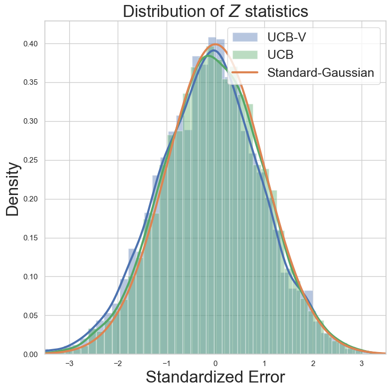
(a) $\Lambda_{T}=0$

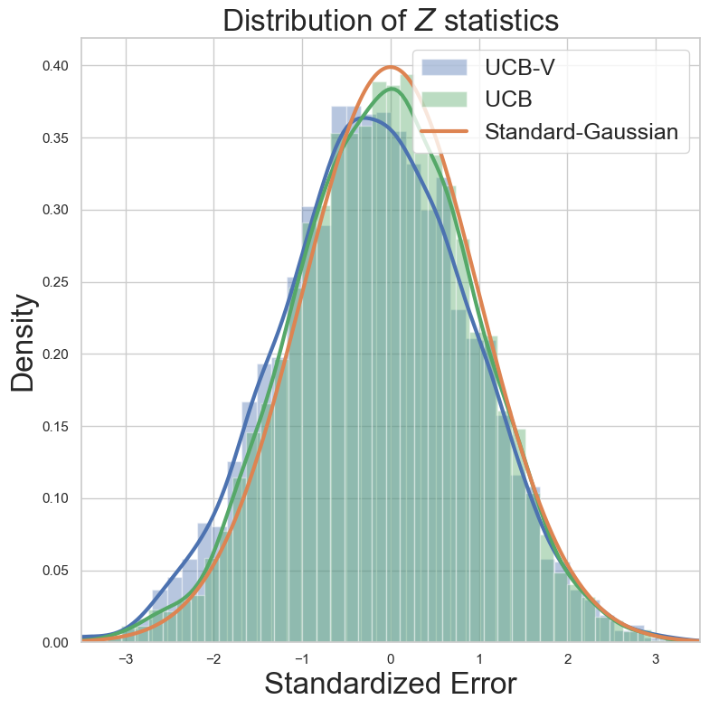
(b) $\Lambda_{T}=1$

Figure 4: The empirical distribution of $Z$-statistic for the sub-optimal arm for UCB and UCB-V with $\sigma_{1}=0,\sigma_{2}=1/4$ under different $\Lambda_{T}$, both with $T=50,000$ and $2,000$ repetitions.

3.3 Unstable results: closer look and hard instances

Recall that Theorem 3 establishes the stability result, except for the case when $\sigma_{1}=\mathfrak{o}(\sigma_{2})$ and $\overline{\sigma}_{2}^{2}/(T\overline{\Delta}_{2})^{2}=1$ hold simultaneously. In this section, we provide a hard instance in this setting and show the instability result. More precisely, consider the setting similar to Example 2, with $\sigma_{2}=1$, $\sigma_{1}=0$ and the gap $\Delta_{2}=\sigma_{2}\sqrt{\theta\log T/T}$. In this scenario, the behavior of the solution of the asymptotic equation is described by $n_{1,T}^{\star}\sim{\lambda^{\star}(\theta)}{T}$, with $\lambda^{\star}(\theta)$ solves:

$$\lambda+\bigg{(}\sqrt{\frac{\rho\log T}{T}}\cdot\frac{1}{\lambda}+\sqrt{\theta/\rho}\bigg{)}^{-2}=1,$$

or equivalently,

$$\frac{1}{\sqrt{1-\lambda}}-\frac{1}{\lambda}\sqrt{\frac{\rho\log T}{T}}=\sqrt{\theta/\rho}.$$ (9)

To heuristically explain why $\theta=\rho$ acts as a phase transition point and its instability, we informally take the first-order expansion $1/\sqrt{1-\lambda}\approx 1+\lambda/2$ in (9) and multiply both sides by $\lambda$. This yields a quadratic equation in $\lambda$:

$$\frac{1}{2}\lambda^{2}+(1-\sqrt{\theta/\rho})\lambda-\sqrt{\frac{\rho\log T}{T}}=0.$$

Notably, the order of the solution in $T$ depends crucially on the sign of $1-\sqrt{\theta/\rho}$. For any $\varepsilon>0$, by observing the analytical solution of the quadratic equation, we have:

$$\lambda=\begin{cases}\mathcal{O}(\varepsilon^{-1}\sqrt{\frac{\rho\log T}{T}})&\text{when }1-\sqrt{\theta/\rho}\geq\varepsilon,\\ \Omega(\varepsilon)&\text{when }1-\sqrt{\theta/\rho}\leq-\varepsilon,\end{cases}$$

In particular, a perturbation in $\theta$ around $\theta=\rho$ of magnitude $\varepsilon$ with different signs can lead to a fluctuation in $n_{1,T}^{\star}$ from $\mathcal{O}(\varepsilon^{-1}\sqrt{T\log T})$ to $\Omega(\varepsilon T)$.

Based on the above intuition and informal argument, we can rigorously demonstrate the instability result by constructing a Bernoulli bandit instance and establishing a time-uniform anti-concentration result for the Bernoulli reward process via Donsker’s principle. Intuitively, our anti-concentration result shows that, with constant probability, $\theta$ can be perturbed by a magnitude of $\mathcal{O}\big{(}1/\log T\big{)}$ with different signs, which then implies instability in $n_{1,T}$ even when we play UCB-V with the oracle information of the variance (i.e. with setting $\widehat{\sigma}_{a,t}=\sigma_{a}$). We summarize the instability result in the following proposition and leave its proof to Section B.3.

Proposition 5.

Consider the following two-armed Bernoulli bandit instance: for $\mu=1/2$ and $\Delta^{2}=\mu(1-\mu)\rho\log T/T$,

• Arm 1 has reward $\mu+\Delta$ and variance 0, and

• Arm 2 has reward $\mu$ and variance $\mu(1-\mu)$.

Suppose $\sigma_{a}$’s are known and let $n_{a,T}$ be computed by Algorithm 1 with $\widehat{\sigma}_{a,t}=\sigma_{a}$. Then for sufficiently large $T$, there exist constants $c_{0},c_{1}>0$ such that

$$\operatorname{\mathbb{P}}(n_{1,T}\leq c_{1}\sqrt{T}\log T)\wedge\operatorname{\mathbb{P}}(n_{1,T}\geq c_{1}^{-1}T/\log^{1/2}T)>c_{0}.$$

The existence of an unstable instance at $\Lambda_{T}=1$ complements our previous finding, where UCB-V’s stability was shown for $\Lambda_{T}\neq 1$. This result highlights a contrast between UCB-V and the canonical UCB: as shown in Kalvit and Zeevi (2021) and Khamaru and Zhang (2024), the canonical UCB is stable for all $\Delta$, which corresponds to the case in our setting where $\sigma_{1}=\sigma_{2}=1$. Our result demonstrates that, in a heterogeneous variance environment, UCB-V may exhibit significant fluctuations. Another implication of this instability is that, unlike the canonical UCB, the CLT for the $Z$-statistic may not hold for data collected by UCB-V, as shown in Figure 4(b). This necessitates the development of new statistical inference methods for UCB-V collected data or new variance-aware decision-making algorithms with stronger stability guarantee than UCB-V, which we leave as a valuable future direction.

4 Refined regret for variance-aware decision making

For UCB-V, Audibert et al. (2009) presents the following gap-dependent upper bound on the arm-pulling number:

$$\mathbb{E}(n_{2,T})\leq C\log T\bigg{(}\frac{\sigma_{2}^{2}}{\Delta_{2}^{2}}+\frac{2}{\Delta_{2}}\bigg{)},$$ (10)

which describes the pulling of sub-optimal arms in the large $\Delta_{2}$ regime, resulting in the regret guarantee $\mathcal{O}\big{(}(\frac{\sigma_{2}^{2}}{\Delta_{2}}\vee 1)\log T\big{)}$ through $\mathrm{Reg}(T)=\Delta_{2}\mathbb{E}(n_{2,T})$.

In this work, we are interested in the worst-case regret, a standard complexity measure, which considers the maximum regret for any $\Delta_{2}\geq 0$. As $\Delta_{2}\to 0$, the bound in (10) becomes vacuous due to the increasing difficulty in distinguishing sub-optimal arms. However, in this regime, decision-making becomes easier as the cost of sub-optimal actions decreases. The trivial bound $\operatorname{\mathbb{E}}(n_{2,T}\Delta_{2})\leq T\Delta_{2}$ becomes effective, yielding the combined result:

$$\mathrm{Reg}(T)\leq\max_{\Delta_{2}\geq 0}C\log T\bigg{(}\frac{\sigma_{2}^{2}}{\Delta_{2}}+2\bigg{)}\wedge\Delta_{2}T\leq C^{\prime}\sigma_{2}\sqrt{T\log T},$$ (11)

where in the last inequality we have used the observation that worst $\Delta_{2}$ is attained at $\Delta_{2}\asymp\sigma_{2}/\sqrt{T\log T}$, leading to the worst-case regret $\mathcal{O}(\sigma_{2}\sqrt{T})$.

As mentioned earlier, the regret in (11) does not account for the effect of $\sigma_{1}$, which contradicts the empirical performance of UCB-V and is conservative in the large $\sigma_{1}$, small $\sigma_{2}$ regime, as shown in Figure 2(a). On the other hand, the derived asymptotic equation for arm-pulling times naturally indicates a dependency of $n_{2,T}$ on $\sigma_{1}$, opening the possibility for refined worst-case regret bounds. A key challenge in applying our asymptotic results to improve regret bounds is the slow convergence rate. The $\mathfrak{o}_{\mathbf{P}}(1)$ term converges to zero with probability $1-\mathcal{O}(1/\log T)$, making it difficult to achieve non-vacuous regret results. The probability of uncontrolled events is $\mathcal{O}(1/\log T)$, which may lead to a regret bound of $\mathcal{O}(T/\log T)$ in expectation. To bypass such limitation, we adopt the high probability bounds in (2) to derive the following Proposition:

Proposition 6.

There exists some universal constant $C_{0}$ such that with $\rho\geq C_{0}$ and $T\geq 3$,

$$\operatorname{\mathbb{P}}\bigg{(}n_{2,T}\leq\frac{16}{\overline{\Delta}_{2}+\varphi(n_{1,T};\overline{\sigma}_{1})}\vee\bigg{(}\frac{16\sigma_{2}}{\overline{\Delta}_{2}+\varphi(n_{1,T};\overline{\sigma}_{1})}\bigg{)}^{2}\bigg{)}\geq 1-\frac{6}{T^{2}}.$$

By applying the upper bound on the number of pulls for sub-optimal arms, we derive the refined worst-case regret for UCB-V:

Theorem 7.

There exists some universal constant $C_{0}>0$ such that for $\rho\geq C_{0}$ and $T\geq 3$, it holds with probability at least $1-6/T^{2}$ that

$$\mathrm{Reg}(T)\leq 16\bigg{(}\sigma_{2}\wedge\frac{16\sigma_{2}^{2}}{\sigma_{1}}\bigg{)}\sqrt{\rho T\log T}+\sqrt{\rho\log T}.$$

The proof of the above results can be found in Section C. The regret bound in Theorem 7 improves upon the bound in (11) for the large $\sigma_{1}$, small $\sigma_{2}$ regime, while recovering the (11) in the small $\sigma_{1}$ regime.

Finally, we conclude by comparing our regret with related works in variance-aware decision making. Since most works consider the general $K$-armed setting, we start by presenting the $K$-armed extension of Theorem 7 for ease of comparison. For the general $K$-armed setting, we have with high probability,

$$\text{Reg}(T)=\mathcal{O}\bigg{(}\sqrt{\sum_{a\in[2:K]}\sigma_{a}^{2}}\wedge\bigg{(}\sum_{a\in[2:K]}\frac{\sigma_{a}^{2}}{\sigma_{1}}\bigg{)}\cdot\sqrt{T\log T}\bigg{)},$$

and a more formal statement can be found in Theorem 9. Firstly, the worst-case regret of UCB-V was previously known as $\mathcal{O}(\sqrt{KT\log T})$, as discussed in Mukherjee et al. (2018). In comparison, our result shows that UCB-V can achieve regret adaptive to both the variance of sub-optimal and optimal arms. Beyond UCB-V, for Thompson sampling algorithms, the $\mathcal{O}(\sqrt{\sum_{a\in[2:K]}\sigma_{a}^{2}T\log T})$ regret was proved in a Bayesian setting, where each arm’s reward distribution follows a known prior distribution. Especially, even when working with the Bayesian regret, the dependency on $\sigma_{1}$ is previously unrevealed. We believe our results for UCB-V can be extended to these posterior sampling algorithms. It is also worth mentioning that another branch of work considers variance-dependent regret for linear bandits, but with different assumptions on variance information. Instead of assuming each arm $a$ has a fixed variance $\sigma_{a}$, they assume that at every round $t$, all arms have the same variance depending on the time-step $t$. Despite this difference, their algorithms can work in our setting with a homogeneous variance assumption: $\sigma_{a}=\sigma,\forall a\in[K]$. In this setting, their result achieves $\mathcal{O}(\sqrt{\sigma KT\log T})$ regret, matching the general form $\sqrt{\sum_{a\in[2:K]}\sigma_{a}^{2}T\log T}$, but still lacking information about $\sigma_{1}$.

5 Discussion on $K$-armed setting

In this section, we extend the results from Theorem 3, which addressed the 2-armed setting, to the general $K$-armed case. Recall that $\overline{\sigma}_{a}\equiv\overline{\sigma}_{a}(\rho;T)$ and $\overline{\Delta}_{a}\equiv\overline{\Delta}_{a}(\rho;T)$ for $a\in[K]$. The formal statement of the result is given in the following theorem.

Theorem 8.

Consider the Algorithm 1. Suppose that for any $a\in[2:K]$,

$$\operatorname*{\overline{lim}}_{T\to\infty}\bigg{\{}\max_{\mathfrak{a}\in[2:K]}\bigg{(}\frac{1}{K-1}-\frac{\overline{\sigma}_{\mathfrak{a}}^{2}}{T\overline{\Delta}_{\mathfrak{a}}^{2}}\bigg{)}_{+}^{-1}\wedge\bigg{(}\frac{\overline{\sigma}_{a}^{2}}{T\overline{\Delta}_{a}^{2}}-1\bigg{)}_{+}^{-1}\wedge\frac{\overline{\sigma}_{a}}{\overline{\sigma}_{1}\vee T^{-1/2}}\bigg{\}}<\infty.$$ (12)

Then for $a\in[K]$, we have

$$\frac{n_{a,T}}{n_{a,T}^{\star}}\xrightarrow{p}1,$$

where $n_{1,T}^{\star}$ is the unique solution to the following equation:

$$\sum_{a\in[K]}\frac{\overline{\sigma}_{a}^{2}\vee(\varphi(n_{1,T}^{\star};\overline{\sigma}_{1})+\overline{\Delta}_{a})}{T(\varphi(n_{1,T}^{\star};\overline{\sigma}_{1})+\overline{\Delta}_{a})^{2}}=1,$$ (13)

and for $a\in[2:K]$,

$$n_{a,T}^{\star}\equiv\frac{\overline{\sigma}_{a}^{2}\vee(\varphi(n_{1,T}^{\star};\overline{\sigma}_{1})+\overline{\Delta}_{a})}{(\varphi(n_{1,T}^{\star};\overline{\sigma}_{1})+\overline{\Delta}_{a})^{2}}.$$

When $K=2$, the condition in (8) simplifies to the stability condition for the $2$-armed setting as stated in Theorem 3. While instability occurs when (8) is violated in the $2$-armed case, cf. Proposition 5, but there is no clear reason to expect that (8) is optimal for the $K$-armed setting. Indeed, as indicated by the proof, the fixed point equation (13) may remain stable if there exists some $a\in[K]\setminus\{1\}$ that satisfies the boundedness condition in (12). However, formally characterizing such an $a$ poses a significant challenge in itself. A full generalization to the $K$-armed setting is left for future work.

Besides the stability results, the high probability bounds for $n_{a,T}$ in the $K$-armed setting, as in (2), still hold when (6) is replaced by (13), as proven in Appendix A. The following corollary provides a refined regret bound in the $K$-armed setting.

Theorem 9.

There exists some universal constant $C_{0}>0$ such that for $\rho\geq C_{0}$ and $T\geq 3$, it holds with probability at least $1-3K/T^{2}$ that

$$\mathrm{Reg}(T)\leq 16\bigg{(}\sqrt{\sum_{a\in[2:K]}\sigma_{a}^{2}}\wedge\sum_{a\in[2:K]}\frac{16\sigma_{a}^{2}}{\sigma_{1}}\bigg{)}\sqrt{\rho T\log T}+(K-1)\sqrt{\rho\log T}.$$

When $K=2$, Theorem 9 aligns with Theorem 7. A comparison with previous findings is provided at the end of the previous section. Notably, in the small $\sigma_{a}^{2}/\sigma_{1}$ regime, the bound in Theorem 9 grows linearly with the number of arms $K$. We conjecture that the result in Theorem 9 is optimal up to logarithmic factors for variance-aware decision-making, even for more complicate algorithms beyond UCB-V. Establishing the corresponding minimax lower bound is left for future work.

Appendix A Proofs for Section 2

For any $T\in\mathbb{N}_{+}$ and $\delta>0$, we define the events

$$\mathcal{M}(\delta;\rho;T)\equiv \bigg{\{}\lvert\bar{X}_{a,t}-\mu_{a}\rvert\leq\varphi_{a,t}\cdot\mathsf{e}(\delta;\rho;T),\;\forall t\in[T],a\in[K]\bigg{\}},$$

$$\mathcal{V}(\delta;\rho;T)\equiv \bigg{\{}\lvert\widehat{\sigma}_{a}^{2}-\sigma_{a}^{2}\rvert\leq\varphi_{a,t}\cdot\mathsf{e}(\delta;\rho;T),\;\forall t\in[T],a\in[K]\bigg{\}}.$$

where $\mathsf{e}(\delta;\rho;T)\equiv\sqrt{48\rho\log T\log(\log(T/\delta)/\delta)}+128\log(1/\delta)$. The majority of the analysis in this paper will be done on the event $\mathcal{M}(\delta;\rho;T)\cap\mathcal{V}(\delta;\rho;T)$. It is worth noting that, as shown in Proposition 20 below, we have $\operatorname{\mathbb{P}}(\mathcal{M}(\delta;\rho;T)\cap\mathcal{V}(\delta;\rho;T))\geq 1-3K\delta$ for any $\delta<1/2$. Although the statements in Section 2 are presented for the $2$-armed setting, the proof in this section applies to the $K$-armed setting as well.

A.1 Proof of Proposition 1

Recall that $\varphi_{a,t}\equiv\varphi(n_{a,t};\overline{\sigma}_{a})$. For simplicity, we denote $\widehat{\varphi}_{a,t}\equiv\varphi(n_{a,t};\widehat{\sigma}_{a,t}/\sqrt{\rho\log T})$ for $a\in[K]$ and $t\in[T]$. The following Lemma provides quantitative error between $\widehat{\varphi}_{a,t}$ and ${\varphi}_{a,t}$.

Lemma 10.

On the event $\mathcal{M}(\delta;\rho;T)\cap\mathcal{V}(\delta;\rho;T)$, we have for any $a\in[K]$ and $t\in[T]$,

$$\lvert\widehat{\varphi}_{a,t}-{\varphi}_{a,t}\rvert\leq{\varphi}_{a,t}\cdot\sqrt{\frac{\mathsf{e}(\delta;\rho;T)}{\rho\log T}}.$$

Proof  By the elementary inequality that $\lvert\sqrt{x}-\sqrt{y}\rvert\leq\sqrt{\lvert x-y\rvert}$ for any $x,y\geq 0$, we may derive on the event $\mathcal{M}(\delta;\rho;T)\cap\mathcal{V}(\delta;\rho;T)$ that

$$\lvert\varphi_{a,t}-\widehat{\varphi}_{a,t}\rvert \leq\frac{\lvert\sigma_{a}-\widehat{\sigma}_{a,t}\rvert}{\sqrt{\rho\log T\cdot n_{a,t}}}=\varphi_{a,t}\cdot\bigg{(}\frac{\lvert\sigma_{a}-\widehat{\sigma}_{a,t}\rvert}{\sqrt{\rho\log T}(\overline{\sigma}_{a}\vee n_{a,t}^{-1/2})}\bigg{)}$$

$$\leq\varphi_{a,t}\cdot\frac{\sqrt{\varphi(n_{a,t};\overline{\sigma}_{a})\cdot\mathsf{e}(\delta;\rho;T)}}{\sqrt{\rho\log T}(\overline{\sigma}_{a}\vee n_{a,t}^{-1/2})}\leq\varphi_{a,t}\cdot\sqrt{\frac{\mathsf{e}(\delta;\rho;T)}{\rho\log T}},$$

which completes the proof.  

Let for any $\delta,\rho>0$, $\mathsf{I}_{\pm}(\delta;\rho;T)\equiv 1\pm\operatorname{\mathsf{Err}}^{1/2}(\delta;\rho;T)\pm\operatorname{\mathsf{Err}}(\delta;\rho;T)$ with $\operatorname{\mathsf{Err}}(\delta;\rho;T)\equiv\mathsf{e}(\delta;\rho;T)/(\rho\log T)$. Recall that $\varphi_{a,T}=\varphi(n_{a,T};\overline{\sigma}_{a})$. The following proposition provides (tight) upper and lower bounds for $\varphi_{a,T}$.

Proposition 11.

Fix any $T\in\mathbb{N}_{+}$ and any $\delta,\rho\in\mathbb{R}_{+}$ such that $\mathsf{I}_{\pm}(\delta;\rho;T)>0$. On the event $\mathcal{M}(\delta;\rho;T)\cap\mathcal{V}(\delta;\rho;T)$, we have for any $a\in[K]$,

$$\frac{\mathsf{I}_{+}(\delta;\rho;T)}{\mathsf{I}_{-}(\delta;\rho;T)}\cdot\frac{n_{a,T}}{n_{a,T}-1}\geq\frac{\overline{\Delta}_{a}+\varphi_{1,T}}{\varphi_{a,T}}\geq\frac{\mathsf{I}_{-}(\delta;\rho;T)}{\mathsf{I}_{+}(\delta;\rho;T)}\cdot\frac{n_{1,T}-1}{n_{1,T}}.$$ (14)

Proof  The proof primarily follows the framework in (Lattimore, 2018; Khamaru and Zhang, 2024). In the proof, we write $\mathsf{I}_{\pm}\equiv\mathsf{I}_{\pm}(\delta;\rho;T)$, $\mathcal{M}\equiv\mathcal{M}(\delta;\rho;T)$, and $\mathcal{V}\equiv\mathcal{V}(\delta;\rho;T)$ for simplicity. For any $a\in[K],$ we denote $T_{a}$ as the last time-step such that the arm $a$ was pulled.

(Step 1). In this step, we provide an upper bound for $\varphi_{a,T}^{-1}$. By the UCB rule,

$$\bar{X}_{a,T_{a}}+\widehat{\varphi}_{a,T_{a}}\cdot{\rho\log T}\geq\bar{X}_{1,T_{a}}+\widehat{\varphi}_{1,T_{a}}\cdot{\rho\log T}.$$

By Lemma 10, on the event $\mathcal{M}\cap\mathcal{V}$,

$$\mathsf{I}_{+}\cdot{\varphi}_{a,T_{a}}\geq\overline{\Delta}_{a}+{\varphi}_{1,T_{a}}\cdot\mathsf{I}_{-}.$$

Using further $n_{a,T_{a}}=n_{a,T}-1$, $n_{1,T_{a}}\leq n_{1,T}$, and $\overline{\Delta}_{a}\geq 0$, we have

$$\mathsf{I}_{+}\cdot\varphi(n_{a,T}-1;\overline{\sigma}_{a})\geq\big{(}\overline{\Delta}_{a}+\varphi_{1,T}\big{)}\cdot\mathsf{I}_{-}.$$

As $\varphi(n_{a,T}-1;\overline{\sigma}_{a})\leq\varphi_{a,T}n_{a,T}/(n_{a,T}-1)$, we obtain an upper bound for $\varphi_{a,T}^{-1}$:

$$\frac{\mathsf{I}_{+}}{\mathsf{I}_{-}}\geq\frac{\overline{\Delta}_{a}+\varphi_{1,T}}{\varphi_{a,T}}\cdot\frac{n_{a,T}-1}{n_{a,T}}.$$ (15)

(Step 2). In this step, we provide a lower bound for $\varphi_{a,T}^{-1}$. Consider the last time-step such that the arm $1$ was pulled, by the UCB rule,

$$\bar{X}_{a,T_{1}}+\widehat{\varphi}_{a,T_{1}}\cdot{\rho\log T}\leq\bar{X}_{1,T_{1}}+\widehat{\varphi}_{1,T_{1}}\cdot{\rho\log T}.$$

By Lemma 10, on the event $\mathcal{M}\cap\mathcal{V}$,

$$\mathsf{I}_{-}\cdot\varphi_{a,T_{1}}\leq\overline{\Delta}_{a}+\varphi_{1,T_{1}}\cdot\mathsf{I}_{+}.$$ (16)

Then by $n_{a,T_{1}}\leq n_{a,T}-1,n_{1,T_{1}}\leq n_{1,T}-1,$ and $\overline{\Delta}_{a}\geq 0$, we have

$$\mathsf{I}_{-}\cdot\varphi_{a,T}\leq\big{(}\overline{\Delta}_{a}+\varphi(n_{1,T}-1;\overline{\sigma}_{1})\big{)}\cdot\mathsf{I}_{+},$$ (17)

As $\varphi(n_{1,T}-1;\overline{\sigma}_{1})\leq\varphi_{1,T}n_{1,T}/(n_{1,T}-1)$, we obtain a lower bound for $\varphi_{a,T}^{-1}$:

$$\frac{\mathsf{I}_{-}}{\mathsf{I}_{+}}\leq\frac{\overline{\Delta}_{a}+\varphi_{1,T}}{\varphi_{a,T}}\cdot\frac{n_{1,T}}{n_{1,T}-1}.$$ (18)

Combining (15) and (18) concludes the proof.  

Proposition 12.

Fix any $T\in\mathbb{N}_{+}$ and any $\delta,\rho\in\mathbb{R}_{+}$ such that $\mathsf{I}_{\pm}(\delta;\rho;T)>0$. On the event $\mathcal{M}(\delta;\rho;T)\cap\mathcal{V}(\delta;\rho;T)$, we have for any $a\in[K]$,

$$\bigg{(}\frac{\mathsf{I}_{+}(\delta;\rho;T)}{\mathsf{I}_{-}(\delta;\rho;T)}\cdot\frac{n_{a,T}}{n_{a,T}-1}\bigg{)}^{-1}\leq\frac{\overline{\sigma}_{a}\vee n_{a,T}^{-1/2}}{\overline{\sigma}_{a}\vee(\varphi_{1,T}+\overline{\Delta}_{a})^{1/2}}\leq\bigg{(}\frac{\mathsf{I}_{-}(\delta;\rho;T)}{\mathsf{I}_{+}(\delta;\rho;T)}\cdot\frac{n_{1,T}-1}{n_{1,T}}\bigg{)}^{-1}.$$

Proof  In the proof below, we write $\mathsf{I}_{\pm}\equiv\mathsf{I}_{\pm}(\delta;\rho;T)$ for simplicity. Let

$${\xi}_{u}\equiv\frac{\mathsf{I}_{+}}{\mathsf{I}_{-}}\cdot\frac{n_{a,T}}{n_{a,T}-1},\quad{\xi}_{l}\equiv\frac{\mathsf{I}_{-}}{\mathsf{I}_{+}}\cdot\frac{n_{1,T}-1}{n_{1,T}}.$$

Note that for any $\sigma>0$, the function $\varphi(\cdot;\sigma):\mathbb{R}_{+}\to\mathbb{R}_{+}$ is bijective and monotone decreasing, with its inverse map given by

$$\psi(z;\sigma):z\to\frac{z\vee\sigma^{2}}{z^{2}},\quad z\in\mathbb{R}_{+}.$$

Starting from the sandwich inequality (14), the monotonicity of $\varphi$ yields that

$$\psi\big{(}{\xi}_{u}^{-1}(\overline{\Delta}_{a}+\varphi_{1,T});\overline{\sigma}_{a}\big{)}\geq n_{a,T}\geq\psi\big{(}\xi_{l}^{-1}(\overline{\Delta}_{a}+\varphi_{1,T});\overline{\sigma}_{a}\big{)}.$$

As $\xi_{l}^{-1}>1$, we have

$$n_{a,T}^{-1}\leq \frac{\xi_{l}^{-2}(\overline{\Delta}_{a}+\varphi_{1,T})^{2}}{\xi_{l}^{-1}(\overline{\Delta}_{a}+\varphi_{1,T})\vee\overline{\sigma}_{a}^{2}}\leq\frac{\xi_{l}^{-2}(\overline{\Delta}_{a}+\varphi_{1,T})^{2}}{(\overline{\Delta}_{a}+\varphi_{1,T})\vee\overline{\sigma}_{a}^{2}}.$$

Using further the fact that $\psi(z;\sigma)^{-1}\vee\sigma^{2}=z\vee\sigma^{2}$, we arrive at

$$n_{a,T}^{-1}\vee\overline{\sigma}_{a}^{2}\leq\big{(}{(\overline{\Delta}_{a}+\varphi_{1,T})\vee\overline{\sigma}_{a}^{2}}\big{)}\cdot\xi_{l}^{-2}.$$

Similar, by $\xi_{u}^{-1}<1$, we may derive that

$$n_{a,T}^{-1}\vee\overline{\sigma}_{a}^{2}\geq\big{(}{(\overline{\Delta}_{a}+\varphi_{1,T})\vee\overline{\sigma}_{a}^{2}}\big{)}\cdot\xi_{u}^{-2}.$$

Combining the above two bounds completes the proof.  

Lemma 13.

Fix any $T\in\mathbb{N}_{+}$ and any $\delta,\rho\in\mathbb{R}_{+}$ such that $0<\mathsf{I}_{+}(\delta;\rho;T)/\mathsf{I}_{-}(\delta;\rho;T)\leq 2$ and $T>2K$. On the event $\mathcal{M}(\delta;\rho;T)\cap\mathcal{V}(\delta;\rho;T)$, we have for any $a\in[K]$

$$n_{a,T}\geq\frac{\sigma_{1}^{2}T\vee\sqrt{T}}{100K}\cdot\bm{1}_{a=1}+\frac{\rho\log T}{8}\cdot\bm{1}_{a\neq 1}.$$ (19)

Proof  In the proof below, we write $\mathsf{I}_{\pm}\equiv\mathsf{I}_{\pm}(\delta;\rho;T)$ for simplicity. We first consider the lower bound for $n_{1,T}$. Suppose by contradiction that (19) does not hold, we have

$$n_{1,T}^{-1/2}>\frac{10\sqrt{K}}{(\overline{\sigma}_{1}\sqrt{T})\vee T^{1/4}},$$

which implies $\overline{\sigma}_{1}\vee n_{1,T}^{-1/2}\geq\overline{\sigma}_{1}\vee(\overline{\sigma}_{1}^{-1}T^{-1/2}\wedge T^{-1/4})=\overline{\sigma}_{1}\vee T^{-1/4}$. Therefore,

$$\varphi_{1,T}=(\overline{\sigma}_{1}\vee n_{1,T}^{-1/2})n_{1,T}^{-1/2}\geq\frac{10\sqrt{K}}{\sqrt{T}}.$$

On the other hand, as $\sum_{a\in[K]}n_{a,T}=T$, there must exist some $a\in[K],a\neq 1$ such that $n_{a,T}\geq T/K$. For such $a$, we have by (15),

$$\frac{\mathsf{I}_{+}}{\mathsf{I}_{-}}\cdot\frac{n_{a,T}}{n_{a,T}-1}\geq\frac{\sqrt{n_{a,T}}\cdot\varphi_{1,T}}{\overline{\sigma}_{1}\vee n_{a,T}^{-1/2}}\Rightarrow\frac{2T}{T-K}\geq\frac{\sqrt{n_{a,T}}\cdot\varphi_{T}}{\overline{\sigma}_{1}\vee n_{a,T}^{-1/2}}$$

$$\Rightarrow\frac{2T}{T-K}\cdot\frac{\overline{\sigma}_{1}\vee n_{a,T}^{-1/2}}{\sqrt{n_{a,T}}}\geq\frac{10\sqrt{K}}{\sqrt{T}}\Rightarrow\frac{2T\sqrt{K}}{T-K}\cdot\frac{1}{\sqrt{T}}\geq\frac{10\sqrt{K}}{\sqrt{T}},$$

which then leads to a contradiction. The lower bound for $n_{1,T}$ follows.

Next, we prove the lower bound for $n_{a,T},a\in[2:K]$. Starting from (18), we have by the lower bound for $n_{1,T}$ in the first part,

$$n_{a,T}\geq\frac{1}{2(\overline{\Delta}_{a}+\varphi_{1,T})}\cdot\frac{n_{1,T}-1}{n_{1,T}}\geq\frac{1}{4}\bigg{(}\frac{1}{\rho\log T}+\frac{10\sqrt{K}}{T^{1/4}}\bigg{)}^{-1}\geq\frac{\rho\log T}{8},$$

proving the claim.  

Now we shall prove Proposition 1

Proof [Proof Proposition 1] In the proof below, we write $\mathsf{I}_{\pm}\equiv\mathsf{I}_{\pm}(\delta;\rho;T)$ and $\operatorname{\mathsf{Err}}\equiv\operatorname{\mathsf{Err}}(\delta;\rho;T)$ for simplicity. It follows from Propositions 11 and 12 that on the event $\mathcal{M}(\delta;\rho;T)\cap\mathcal{V}(\delta;\rho;T)$,

$$\frac{\mathsf{I}_{-}^{2}}{\mathsf{I}_{+}^{2}}\cdot\frac{(n_{a,T}-1)(n_{1,T}-1)}{n_{a,T}n_{1,T}} \leq\frac{\sqrt{n_{a,T}}\cdot(\overline{\Delta}_{a}+\varphi_{1,T})}{\overline{\sigma}_{a}\vee(\varphi_{1,T}+\overline{\Delta}_{a})^{1/2}}\leq\frac{\mathsf{I}_{+}^{2}}{\mathsf{I}_{-}^{2}}\cdot\frac{n_{a,T}n_{1,T}}{(n_{a,T}-1)(n_{1,T}-1)}.$$

Applying the lower bounds for $n_{a,T}$ in Lemma 13, we may further bound the right hand side as follows:

$$\frac{\mathsf{I}_{+}^{2}}{\mathsf{I}_{-}^{2}}\cdot\bigg{(}1-\frac{8}{\rho\log T}\bigg{)}^{-1}\cdot\bigg{(}1-\frac{100K}{\sqrt{T}}\bigg{)}^{-1}$$

$$\leq\bigg{(}\frac{1+2\sqrt{\operatorname{\mathsf{Err}}}}{1-2\sqrt{\operatorname{\mathsf{Err}}}}\bigg{)}^{2}\bigg{(}1-\frac{8}{\rho\log T}\bigg{)}^{-1}\bigg{(}1-\frac{100K}{\sqrt{T}}\bigg{)}^{-1}\leq\frac{(1+2\sqrt{\operatorname{\mathsf{Err}}})^{2}}{1-5\sqrt{\operatorname{\mathsf{Err}}}-100KT^{-1/2}},$$

where we use $\sqrt{\operatorname{\mathsf{Err}}}\geq 8/(\rho\log T)$ and the elementary inequality $(1-x)(1-y)(1-z)\geq 1-x-y-z$ for $\forall x,y,z>0$.

Using the same argument for the left hand side, we have

$$\frac{1-5\sqrt{\operatorname{\mathsf{Err}}}-100KT^{-1/2}}{(1+2\sqrt{\operatorname{\mathsf{Err}}})^{2}} \leq\frac{\sqrt{n_{a,T}}\cdot(\overline{\Delta}_{a}+\varphi_{1,T})}{\overline{\sigma}_{a}\vee(\varphi_{1,T}+\overline{\Delta}_{a})^{1/2}}\leq\frac{(1+2\sqrt{\operatorname{\mathsf{Err}}})^{2}}{1-5\sqrt{\operatorname{\mathsf{Err}}}-100KT^{-1/2}}.$$

Summing over $a$ and using the fact that $\sum_{a\in[K]}n_{a,T}=T,$ we obtain

$$\frac{(1-5\sqrt{\operatorname{\mathsf{Err}}}-100KT^{-1/2})^{2}}{(1+2\sqrt{\operatorname{\mathsf{Err}}})^{4}}\leq\sum_{a=1}^{K}\frac{\overline{\sigma}_{a}^{2}\vee(\varphi_{1,T}+\overline{\Delta}_{a})}{T(\overline{\Delta}_{a}+\varphi_{1,T})^{2}}\leq\frac{(1+2\sqrt{\operatorname{\mathsf{Err}}})^{4}}{(1-5\sqrt{\operatorname{\mathsf{Err}}}-100KT^{-1/2})^{2}},$$

as desired.  

Appendix B Proofs for Section 3

B.1 Proof of Lemma 2

Proof [Proof of Lemma 2] (1). First we prove the existence and uniqueness of $\varphi^{\star}$. Note that $f(\varphi)$ is continuously monotone decreasing on $(0,\infty)$. On the other hand, as

$$f(1/T)=\frac{\overline{\sigma}_{1}^{2}\vee T^{-1}}{T^{-1}}+\frac{\overline{\sigma}_{2}^{2}\vee(T^{-1}+\overline{\Delta}_{2})}{T(T^{-1}+\overline{\Delta}_{2})^{2}}>\frac{\overline{\sigma}_{1}^{2}\vee T^{-1}}{T^{-1}}\geq 1,$$

and

$$f(1)=\frac{\overline{\sigma}_{1}^{2}\vee 1}{T}+\frac{\overline{\sigma}_{2}^{2}\vee(1+\overline{\Delta}_{2})}{T(1+\overline{\Delta}_{2})^{2}}\leq\frac{2}{T}<1,$$

there must exist a unique $\varphi^{\star}\in(1/T,1)$ such that $f(\varphi^{\star})=1$, proving the claim.

(2). We only show the proof for the case of $\delta>0$ while the case $\delta<0$ can be handled similarly. Note by monotonicity, we have $\varphi_{\delta}\leq\varphi^{\star}$. Let $\varphi_{\delta}/\varphi^{\star}=1-\bar{\delta}$ for some $\bar{\delta}=\bar{\delta}(\delta)\geq 0$. Our aim is to derive an upper bound for $\bar{\delta}$.

It follows from (3) that at least one of the following holds:

$$\textbf{Case 1}:\leavevmode\nobreak\ \frac{\overline{\sigma}_{1}^{2}\vee\varphi^{\star}}{T(\varphi^{\star})^{2}}\geq\frac{1}{2},\quad\textbf{Case 2}:\leavevmode\nobreak\ \frac{\overline{\sigma}_{2}^{2}\vee(\varphi^{\star}+\overline{\Delta}_{2})}{T(\varphi^{\star}+\overline{\Delta}_{2})^{2}}\geq\frac{1}{2}.$$

Case 1: If $\overline{\sigma}_{1}^{2}=\overline{\sigma}_{1}^{2}\vee\varphi^{\star}$, we have $\overline{\sigma}_{1}^{2}=\overline{\sigma}_{1}^{2}\vee\varphi_{\delta}$. Therefore,

$$\delta =f(\varphi_{\delta})-f(\varphi^{\star})\geq\frac{\overline{\sigma}_{1}^{2}\vee\varphi_{\delta}}{T\varphi_{\delta}^{2}}-\frac{\overline{\sigma}_{1}^{2}\vee\varphi^{\star}}{T(\varphi^{\star})^{2}}=\frac{\overline{\sigma}_{1}^{2}}{T(\varphi^{\star})^{2}}\bigg{(}\frac{1-(1-\bar{\delta})^{2}}{(1-\bar{\delta})^{2}}\bigg{)}\geq\frac{1}{2}\bar{\delta}.$$

For the case when $\varphi^{\star}=\overline{\sigma}_{1}^{2}\vee\varphi^{\star}$, we may compute that

$$\delta =f(\varphi_{\delta})-f(\varphi^{\star})\geq\frac{\overline{\sigma}_{1}^{2}\vee\varphi_{\delta}}{T\varphi_{\delta}^{2}}-\frac{\overline{\sigma}_{1}^{2}\vee\varphi^{\star}}{T(\varphi^{\star})^{2}}\geq\frac{1}{T\varphi^{\star}}\bigg{(}1-\frac{1}{1-\bar{\delta}}\bigg{)}\geq\frac{1}{2}\bar{\delta}.$$

By combining the above results, in Case 1, we conclude that $\bar{\delta}\leq 2\delta$.

Case 2: Note that in this case, we have

$$\frac{1}{T\varphi^{\star}}\vee\frac{\overline{\sigma}_{1}^{2}}{T(\varphi^{\star})^{2}}\leq\frac{\overline{\sigma}_{1}^{2}\vee\varphi^{\star}}{T(\varphi^{\star})^{2}}\leq\frac{1}{2}.$$ (20)

On the other hand, if $\varphi^{\star}+\overline{\Delta}_{2}=\overline{\sigma}_{2}^{2}\vee(\varphi^{\star}+\overline{\Delta}_{2})$, we can show that $1/(T\varphi^{\star})\geq 1/T(\varphi^{\star}+\overline{\Delta}_{2})\geq 1/2$. Therefore, it must hold that $\varphi^{\star}=T/2$ and $\overline{\Delta}_{2}=0$. This implies that when $\varphi^{\star}+\overline{\Delta}_{2}=\overline{\sigma}_{2}^{2}\vee(\varphi^{\star}+\overline{\Delta}_{2})$,

$$\delta=f(\varphi_{\delta})-f(\varphi^{\star}) \geq\frac{1}{T(\varphi_{\delta}+\overline{\Delta}_{2})}-\frac{1}{T(\varphi^{\star}+\overline{\Delta}_{2})}$$

$$=\frac{1}{T\varphi^{\star}}\bigg{(}1-\frac{1}{1-\bar{\delta}}\bigg{)}\geq\frac{1}{2}\bar{\delta}.$$

For the case when $\overline{\sigma}_{2}^{2}=\overline{\sigma}_{2}^{2}\vee(\varphi^{\star}+\overline{\Delta}_{2})$, using (20) and the fact that $\varphi^{\star}\geq T^{-1}$, we have

$$\frac{\overline{\sigma}_{2}^{2}}{T(\varphi^{\star}+\overline{\Delta}_{2})^{2}}\geq\frac{1}{2}\geq\frac{\overline{\sigma}_{1}^{2}\vee\varphi^{\star}}{T(\varphi^{\star})^{2}}\geq\frac{\overline{\sigma}_{1}^{2}\vee T^{-1}}{T(\varphi^{\star})^{2}},$$

which implies that $\varphi^{\star}/(\varphi^{\star}+\overline{\Delta}_{2})\geq(\overline{\sigma}_{1}\vee T^{-1/2})/\overline{\sigma}_{2}$. Therefore,

$$\delta =f(\varphi_{\delta})-f(\varphi^{\star})\geq\frac{\overline{\sigma}_{2}^{2}}{T(\varphi_{\delta}+\overline{\Delta}_{2})^{2}}-\frac{\overline{\sigma}_{2}^{2}}{T(\varphi^{\star}+\overline{\Delta}_{2})^{2}}$$ (21)

$$=\frac{\overline{\sigma}_{2}^{2}(\varphi^{\star}-\varphi_{\delta})}{T(\varphi^{\star}+\overline{\Delta}_{2})^{2}}\cdot\bigg{(}\frac{\varphi_{\delta}+\varphi^{\star}+2\overline{\Delta}_{2}}{(\varphi_{\delta}+\overline{\Delta}_{2})^{2}}\bigg{)}\geq\frac{\varphi^{\star}\bar{\delta}}{2(\varphi^{\star}+\overline{\Delta}_{2})}\geq\frac{\overline{\sigma}_{1}\vee T^{-1/2}}{2\overline{\sigma}_{2}}\bar{\delta}.$$

This gives the bound corresponds to ${\overline{\sigma}_{2}}/(\overline{\sigma}_{1}\vee T^{-1/2})$ in (4).

Next, we shall derive the bound corresponds to $\lvert\overline{\sigma}_{2}^{2}/(T\overline{\Delta}_{2}^{2})-1\rvert^{-1}$ in (4). The analysis will be further separated into two cases: (i) $1-\overline{\sigma}_{2}^{2}/(T\overline{\Delta}_{2}^{2})\geq 0$ and (ii) $1-\overline{\sigma}_{2}^{2}/(T\overline{\Delta}_{2}^{2})<0$.

For (i), we have

$$\delta =f(\varphi_{\delta})-f(\varphi^{\star})\geq\frac{\bar{\delta}}{1-\bar{\delta}}\cdot\frac{\overline{\sigma}_{1}^{2}\vee\varphi^{\star}}{T(\varphi^{\star})^{2}}+\bar{\delta}\cdot\frac{\overline{\sigma}_{2}^{2}\varphi^{\star}}{T(\varphi^{\star}+\overline{\Delta}_{2})^{3}}$$

$$\geq\bigg{(}\frac{\overline{\sigma}_{1}^{2}\vee\varphi^{\star}}{T(\varphi^{\star})^{2}}+\frac{\overline{\sigma}_{2}^{2}}{T(\varphi^{\star}+\overline{\Delta}_{2})^{2}}-\frac{\overline{\sigma}_{2}^{2}\overline{\Delta}_{2}}{T(\varphi^{\star}+\overline{\Delta}_{2})^{3}}\bigg{)}\cdot\bar{\delta}\geq\bigg{(}1-\frac{\overline{\sigma}_{2}^{2}}{T\overline{\Delta}_{2}^{2}}\bigg{)}\cdot\bar{\delta}.$$

For (ii), we recall from (21) that

$$\delta \geq\frac{\varphi^{\star}\bar{\delta}}{2(\varphi^{\star}+\overline{\Delta}_{2})}\geq\frac{\bar{\delta}}{6}\cdot\bm{1}_{\overline{\Delta}_{2}/\varphi^{\star}\leq 2}+\frac{\varphi^{\star}\bar{\delta}}{2(\varphi^{\star}+\overline{\Delta}_{2})}\cdot\bm{1}_{\overline{\Delta}_{2}/\varphi^{\star}>2}.$$ (22)

Note that when $\overline{\Delta}_{2}/\varphi^{\star}>2$ (or equivalently $\varphi^{\star}/\overline{\Delta}_{2}<1/2$),

$$\frac{\overline{\sigma}_{2}^{2}}{T(\varphi^{\star}+\overline{\Delta}_{2})^{2}}\geq\frac{\overline{\sigma}_{2}^{2}}{T\overline{\Delta}_{2}^{2}}\bigg{(}1-3\frac{\varphi^{\star}}{\overline{\Delta}_{2}}\bigg{)}\;\Rightarrow\;\bigg{(}\frac{\overline{\sigma}_{2}^{2}}{T\overline{\Delta}_{2}^{2}}-1\bigg{)}\frac{1}{\varphi^{\star}}-\frac{3\overline{\sigma}_{2}^{2}}{T\overline{\Delta}_{2}^{3}}\leq 0.$$

Using the condition that $1-\overline{\sigma}_{2}^{2}/(T\overline{\Delta}_{2}^{2})<0$, we may derive

$$(\varphi^{\star})^{-1}\overline{\Delta}_{2}\leq\frac{3\overline{\sigma}_{2}^{2}}{T\overline{\Delta}_{2}^{2}}\cdot\bigg{(}\frac{\overline{\sigma}_{2}^{2}}{T\overline{\Delta}_{2}^{2}}-1\bigg{)}^{-1}.$$

As $\overline{\sigma}_{2}^{2}/(\varphi^{\star}+\overline{\Delta}_{2})^{2}\leq T$ and $\varphi^{\star}/\overline{\Delta}_{2}<1/2$, we may obtain that $\overline{\sigma}_{2}^{2}/(T\overline{\Delta}_{2}^{2})\leq 9/4$, which then implies $(\varphi^{\star})^{-1}\overline{\Delta}_{2}\leq 27/(2\overline{\sigma}_{2}^{2}/(T\overline{\Delta}_{2}^{2})-2)$. Therefore,

$$\frac{\varphi^{\star}\bar{\delta}}{2(\varphi^{\star}+\overline{\Delta}_{2})}\cdot\bm{1}_{\overline{\Delta}_{2}/\varphi^{\star}>2}\geq\frac{\bar{\delta}}{2+27\Big{(}\frac{\overline{\sigma}_{2}^{2}}{T\overline{\Delta}_{2}^{2}}-1\Big{)}^{-1}}\cdot\bm{1}_{\overline{\Delta}_{2}/\varphi^{\star}>2}.$$

Plugging this back to (22) yields

$$\delta\geq\frac{\bar{\delta}}{6+27\Big{(}\frac{\overline{\sigma}_{2}^{2}}{T\overline{\Delta}_{2}^{2}}-1\Big{)}^{-1}}.$$

By combining the above results, in Case 2, we conclude that

$$\bar{\delta}\leq 27\delta\cdot\bigg{(}1+\bigg{\lvert}\frac{\overline{\sigma}_{2}^{2}}{T\overline{\Delta}_{2}^{2}}-1\bigg{\rvert}^{-1}\wedge\frac{\overline{\sigma}_{2}}{\overline{\sigma}_{1}\vee T^{-1/2}}\bigg{)}.$$

The claim then follows by combining the estimates in Case 1 and Case 2.  

B.2 Proof of Theorem 3

Proposition 14.

For any positive sequences $\{\sigma_{T}\}_{T\geq 1},\{n_{T}\}_{T\geq 1},\{\bar{n}_{T}\}_{T\geq 1}$, the following are equivalent:

1. $\lim_{T\to\infty}\varphi(n_{T};\sigma_{T})/\varphi(\bar{n}_{T};\sigma_{T})=1$.

2. $\lim_{T\to\infty}n_{T}/\bar{n}_{T}=1$.

Proof  (1) $\Rightarrow$ (2). First note by the elementary inequality

$$1\wedge\frac{a}{b}\leq\frac{a\vee c}{b\vee c}\leq 1\vee\frac{a}{b},\quad\forall a,b,c>0,$$ (23)

we may deduce from (1) that $\lim_{T\to\infty}(\varphi(n_{T};\sigma_{T})\vee\sigma_{T}^{2})/(\varphi(\bar{n}_{T};\sigma_{T})\vee\sigma_{T}^{2})=1$. Using further the identity $n=(\sigma^{2}\vee\varphi(n;\sigma))/\varphi^{2}(n;\sigma)$ for any $n,\sigma>0$, we have

$$\lim_{T\to\infty}\frac{n_{T}}{\bar{n}_{T}}=\bigg{(}\lim_{T\to\infty}\frac{\varphi^{2}(n_{T};\sigma_{T})}{\varphi^{2}(\bar{n}_{T};\sigma_{T})}\bigg{)}\cdot\bigg{(}\lim_{T\to\infty}\frac{\varphi({n}_{T};\sigma_{T})\vee\sigma_{T}^{2}}{\varphi(\bar{n}_{T};\sigma_{T})\vee\sigma_{T}^{2}}\bigg{)}=1.$$

(2) $\Rightarrow$ (1). By (23), we have (2) implies $\lim_{T\to\infty}(\sigma_{T}\vee n_{T}^{-1/2})/(\sigma_{T}\vee\bar{n}_{T}^{-1/2})=1$. Consequently,

$$\lim_{T\to\infty}\frac{\varphi(n_{T};\sigma_{T})}{\varphi(\bar{n}_{T};\sigma_{T})}=\bigg{(}\lim_{T\to\infty}\sqrt{\frac{{\bar{n}_{T}}}{{n_{T}}}}\bigg{)}\cdot\bigg{(}\lim_{T\to\infty}\frac{\sigma_{T}\vee n_{T}^{-1/2}}{\sigma_{T}\vee\bar{n}_{T}^{-1/2}}\bigg{)}=1.$$

The claim follows.  

Now we shall prove Theorem 3.

Proof [Proof of Theorem 3] Selecting $\delta=1/\log T$. In the proof, we write $\mathsf{I}_{\pm}\equiv\mathsf{I}_{\pm}(\delta;\rho;T)$, $\mathcal{M}\equiv\mathcal{M}(\delta;\rho;T)$, and $\mathcal{V}\equiv\mathcal{V}_{T}(\delta;\rho;T)$ for simplicity. We also write $\varphi^{\star}\equiv\varphi(n_{1,T}^{\star};\overline{\sigma}_{1})$. By Proposition 20, we have $\operatorname{\mathbb{P}}(\mathcal{M}\cap\mathcal{V})\geq 1-3K/\log T$.

The uniqueness of $n_{1,\star}$ directly follows from Lemma 2-(1) and the fact that $\varphi(\cdot;\overline{\sigma}_{1})$ is bijective. By Propositions 11 and 12, we have on the event $\mathcal{M}\cap\mathcal{V}$ that

$$\frac{\mathsf{I}_{-}^{2}}{\mathsf{I}_{+}^{2}}\cdot\frac{(n_{a,T}-1)(n_{1,T}-1)}{n_{a,T}n_{1,T}} \leq\frac{\sqrt{n_{a,T}}\cdot(\overline{\Delta}_{a}+\varphi_{1,T})}{\overline{\sigma}_{a}\vee(\varphi_{1,T}+\overline{\Delta}_{a})^{1/2}}\leq\frac{\mathsf{I}_{+}^{2}}{\mathsf{I}_{-}^{2}}\cdot\frac{n_{a,T}n_{1,T}}{(n_{a,T}-1)(n_{1,T}-1)}.$$

Applying Lemma 13 and using the facts that $\varphi_{1,T}=\mathfrak{o}(1)$ on $\mathcal{M}\cap\mathcal{V}$ and $\overline{\Delta}_{a}=\mathfrak{o}(1)$, we have for any $a\in[K]$, $\lim_{T\to\infty}n_{a,T}=+\infty$ on $\mathcal{M}\cap\mathcal{V}$. Therefore, the inequality in the above display implies that for any $a\in[K]$,

$$n_{a,T}\cdot\frac{(\varphi_{1,T}+\overline{\Delta}_{a})^{2}}{\overline{\sigma}_{a}^{2}\vee(\varphi_{1,T}+\overline{\Delta}_{a})}=1+\mathfrak{o}_{\mathbf{P}}(1).$$ (24)

Using further $\sum_{a\in[K]}n_{a,T}/T=1$, we arrive at

$$\sum_{a\in[K]}\frac{\overline{\sigma}_{a}^{2}\vee(\varphi_{1,T}+\overline{\Delta}_{a})}{T(\varphi_{1,T}+\overline{\Delta}_{a})^{2}}=1+\mathfrak{o}_{\mathbf{P}}(1).$$ (25)

Consider the case when $K=2$, it follows from Lemma 2-(2) that $\varphi_{1,T}/\varphi^{\star}=1+\mathfrak{o}_{\mathbf{P}}(1)$, which together with Proposition 14, implies that $n_{1,T}/n_{1,T}^{\star}=1+\mathfrak{o}_{\mathbf{P}}(1)$.

For arm $2$, with (24) at hand, by Proposition 14, it suffices to show that

$$\frac{\varphi_{1,T}}{\varphi^{\star}}=1+\mathfrak{o}_{\mathbf{P}}(1)\;\Rightarrow\;\frac{\overline{\sigma}_{2}^{2}\vee(\varphi^{\star}+\overline{\Delta}_{2})}{\overline{\sigma}_{2}^{2}\vee(\varphi_{1,T}+\overline{\Delta}_{2})}\cdot\frac{(\varphi_{1,T}+\overline{\Delta}_{2})^{2}}{(\varphi^{\star}+\overline{\Delta}_{2})^{2}}=1+\mathfrak{o}_{\mathbf{P}}(1),$$

which is straightforward by (23).  

B.3 Proof of Proposition 5

We need the following lemma to prove Proposition 5.

Lemma 15.

Consider the Two-armed Bernoulli Bandit instance in Proposition 5. Recall that $T_{i}$ is the last time that Arm $i$ was pulled. Then for sufficiently large $T$, there exists some constants $c_{0}>0$ such that

$$\operatorname{\mathbb{P}}\bigg{(}\mathcal{U}\equiv\Big{\{}\bar{X}_{2,T_{1}}>\frac{1}{2}+\frac{1}{\sqrt{n_{2,T_{1}}}}\Big{\}}\bigg{)}\wedge\operatorname{\mathbb{P}}\bigg{(}\mathcal{L}\equiv\Big{\{}\bar{X}_{2,T_{2}}<\frac{1}{2}-\frac{1}{\sqrt{n_{2,T_{2}}}}\Big{\}}\bigg{)}\geq c_{0}.$$

Proof  (Step 1). We first prove the following: On the event $\mathcal{M}_{T}\cap\mathcal{V}_{T}$, there exists some constants $0<c<1$ such that

$$n_{2,T_{1}\wedge T_{2}}\geq cT.$$ (26)

To this end, recalling from (16) that

$$\frac{\mathsf{I}_{-}}{2\sqrt{n_{2,T_{1}}}}\leq\frac{1}{2\sqrt{T}}+\frac{\mathsf{I}_{+}}{n_{1,T_{1}}}$$

holds on the event $\mathcal{M}(1/\log T;\rho;T)\cap\mathcal{V}(1/\log T;\rho;T)$ and using Lemma 13 with the fact that $n_{1,T_{1}}=n_{1,T}-1$, we may estimate for sufficiently large $T$ that

$$n_{2,T_{1}}\gtrsim\bigg{(}\frac{1}{\sqrt{T}}+\frac{1}{n_{1,T_{1}}}\bigg{)}^{-2}\gtrsim T.$$

Given that $n_{2,T_{2}}=n_{2,T}-1$, a similar estimate applies to $n_{2,T_{2}}$ if we start from (17), proving (26).

(Step 2). Let $c$ be the constant in (26). It follows from Step 1 and Lemma 19 that for any $\varepsilon>0$, there exists some $T_{0}=T_{0}(\varepsilon)>0$ such that for $T\geq T_{0}$, $\operatorname{\mathbb{P}}(n_{2,T_{1}}\geq cT)\geq 1-\varepsilon$. Using Lemma 21 and choosing $\varepsilon=c_{\text{anti}}/2$, we have

$$\operatorname{\mathbb{P}}(\mathcal{U})\geq\operatorname{\mathbb{P}}\bigg{(}\Big{\{}\bar{X}_{2,T_{1}}>\frac{1}{2}+\frac{1}{\sqrt{n_{2,T_{1}}}}\Big{\}}\cap\{n_{2,T_{1}}\geq\lfloor cT\rfloor\}\bigg{)}$$

$$\geq\operatorname{\mathbb{P}}\Bigg{(}\bigg{\{}\sum_{i\in[n]}X_{i}>\frac{n}{2}+\sqrt{n}\text{ for all }n\geq\lfloor cT\rfloor\bigg{\}}\cap\{n_{2,T_{1}}\geq\lfloor cT\rfloor\}\Bigg{)}\geq c_{\text{anti}}-\varepsilon\geq\frac{c_{\text{anti}}}{2}.$$

This concludes the proof for the probability estimate for $\mathcal{U}$. The estimate for $\operatorname{\mathbb{P}}(\mathcal{L})$ follows a similar argument, so will be omitted to avoid repetitive details.  

Now we shall prove Proposition 5.

Proof [Proof of Proposition 5] (1). We first prove the upper bound for $n_{1,T}$ on the event $\mathcal{U}\cap\mathcal{M}(1/\log T;\rho;T)\cap\mathcal{V}(1/\log T;\rho;T)$. Consider the time $T_{1}$ that the arm $1$ was last pulled, using (i) the definition of $\mathcal{U}$ and (ii) the UCB rule, we have on the event $\mathcal{U}\cap\mathcal{M}(1/\log T;\rho;T)\cap\mathcal{V}(1/\log T;\rho;T)$,

$$\mu+\frac{1}{\sqrt{n_{2,T_{1}}}}+{\varphi}_{2,T_{1}}\cdot\rho\log T\overset{\mathrm{(i)}}{\leq}\bar{X}_{2,T_{1}}+{\varphi}_{2,T_{1}}\cdot\rho\log T\overset{\mathrm{(ii)}}{\leq}\mu+\Delta+\frac{{\rho\log T}}{n_{1,T_{1}}}.$$

Rearranging the terms, on the event $\mathcal{U}\cap\mathcal{M}(1/\log T;\rho;T)\cap\mathcal{V}(1/\log T;\rho;T)$,

$${\varphi}_{2,T_{1}}\cdot\rho\log T\leq\Delta-\frac{1}{\sqrt{n_{2,T_{1}}}}+\frac{{\rho\log T}}{n_{1,T_{1}}}.$$

By the facts that $\sigma_{2}^{2}=\mu(1-\mu)$, $\Delta^{2}=\mu(1-\mu)\rho\log T/T$, $n_{2,T}\geq n_{2,T_{1}}$, $n_{1,T_{1}}=n_{1,T_{1}}-1$, and $n_{1,T}+n_{2,T}=T$, we arrive at

$$\frac{1}{n_{1,T}-1}-\bigg{(}1+\frac{1}{\rho\overline{\sigma}_{2}{\log T}}\bigg{)}\cdot\frac{\overline{\sigma}_{2}}{\sqrt{T-n_{1,T}}}\geq-\frac{\overline{\sigma}_{2}}{\sqrt{T}}$$

Further using $1/\sqrt{T-n_{1,T}}\geq(1+n_{1,T}/(2T))/\sqrt{T}$, the above inequality becomes

$$\frac{1}{n_{1,T}-1}-\bigg{(}1+\frac{1}{\rho\overline{\sigma}_{2}{\log T}}\bigg{)}\cdot\frac{\overline{\sigma}_{2}n_{1,T}}{2T^{3/2}}\geq\frac{1}{\rho\overline{\sigma}_{2}{\log T}}\cdot\frac{\overline{\sigma}_{2}}{\sqrt{T}}.$$

Note that the above inequality is quadratic, we may then solve it to yield:

$$n_{1,T}\leq\frac{\sqrt{(\overline{B}-\overline{A})^{2}+4\overline{A}(\overline{B}+1)}-(\overline{B}-\overline{A})}{2\overline{A}},$$

where for sufficiently large $T$,

$$\overline{A} =\bigg{(}1+\frac{1}{\rho\overline{\sigma}_{2}{\log T}}\bigg{)}\cdot\frac{\overline{\sigma}_{2}}{2T^{3/2}}\asymp\frac{1}{T\sqrt{T\log T}},$$

$${\overline{B}} ={\frac{1}{\rho\overline{\sigma}_{2}{\log T}}}\cdot\frac{\overline{\sigma}_{2}}{\sqrt{T}}\asymp\frac{1}{\sqrt{T}\log T}.$$

Therefore, we may conclude on the event $\mathcal{U}\cap\mathcal{M}(1/\log T;\rho;T)\cap\mathcal{V}(1/\log T;\rho;T)$ that

$$n_{1,T}\leq\frac{2(\overline{B}+1)}{\sqrt{(\overline{B}-\overline{A})^{2}+4\overline{A}(\overline{B}+1)}+(\overline{B}-\overline{A})}\leq\frac{2({\overline{B}}+1)}{{\overline{B}-\overline{A}}}\lesssim\sqrt{T}\log T.$$

(2). The lower bound for $n_{1,T}$ on the event $\mathcal{L}\cap\mathcal{M}(1/\log T;\rho;T)\cap\mathcal{V}(1/\log T;\rho;T)$ is made by a similar strategy. Consider the time $T_{2}$ that the arm $2$ was last pulled, using (i) the definition of $\mathcal{L}$ and (ii) the UCB rule, we have on the event $\mathcal{L}\cap\mathcal{M}(1/\log T;\rho;T)\cap\mathcal{V}(1/\log T;\rho;T)$,

$$\mu-\frac{1}{\sqrt{n_{2,T_{2}}}}+\varphi_{2,T_{2}}\cdot\rho\log T\overset{\mathrm{(i)}}{\geq}\bar{X}_{2,T_{2}}+{\varphi}_{2,T_{2}}\cdot\rho\log T\overset{\mathrm{(ii)}}{\geq}\mu+\Delta+\frac{{\rho\log T}}{n_{1,T_{2}}}.$$

Rearranging the terms, on the event $\mathcal{L}\cap\mathcal{M}(1/\log T;\rho;T)\cap\mathcal{V}(1/\log T;\rho;T)$,

$$\varphi_{2,T_{2}}\cdot\rho\log T\geq\Delta+\frac{1}{\sqrt{n_{2,T_{2}}}}+\frac{{\rho\log T}}{n_{1,T_{2}}}.$$

By the facts that $\overline{\Delta}_{2}^{2}=\overline{\sigma}_{2}^{2}/T$, $n_{1,T}\geq n_{1,T_{2}}$, $n_{2,T_{2}}=n_{2,T}-1$, and $n_{1,T}+n_{2,T}=T$, we arrive at

$$\frac{1}{n_{1,T}}-\bigg{(}1-\frac{1}{{\rho\overline{\sigma}_{2}\log T}}\bigg{)}\cdot\frac{\overline{\sigma}_{2}}{\sqrt{T-n_{1,T}-1}}\leq-\frac{\overline{\sigma}_{2}}{\sqrt{T}}.$$

Note that on the event $\mathcal{L}\cap\mathcal{M}(1/\log T;\rho;T)\cap\mathcal{V}(1/\log T;\rho;T)$, $c_{1}\sqrt{T}\leq n_{1,T}+1\leq c_{2}T$ for some constants $c_{1}>0$ and $0<c_{2}<1$, cf. Lemme 13 and (26), we may then derive for sufficiently large $T$,

$$\frac{1}{n_{1,T}}-\bigg{(}1-\frac{1}{{\rho\overline{\sigma}_{2}\log T}}\bigg{)}\cdot\frac{\overline{\sigma}_{2}}{\sqrt{T}}\cdot\bigg{(}1+\frac{2n_{1,T}}{(1-c_{2})T}\bigg{)}\leq-\frac{\overline{\sigma}_{2}}{\sqrt{T}},$$ (27)

where we also used $1/\sqrt{1-(n_{1,T}+1)/T}\leq 1+2n_{1,T}/(1-c_{2})T$. Then with

$$\underline{A} =\frac{2\overline{\sigma}_{2}}{(1-c_{2})T^{3/2}}\bigg{(}1-\frac{1}{{\rho\overline{\sigma}_{2}\log T}}\bigg{)}\asymp\frac{1}{T\sqrt{T\log T}},$$ (28)

$$\underline{B} =\frac{1}{{\rho\overline{\sigma}_{2}\log T}}\cdot\frac{\overline{\sigma}_{2}}{\sqrt{T}}\asymp\frac{1}{\sqrt{T}\log T},$$ (29)

we may solve the inequality (27) to yield:

$$n_{1,T}\geq\frac{\underline{B}+\sqrt{\underline{B}^{2}+4\underline{A}}}{2\underline{A}}\geq\frac{\underline{B}}{2\underline{A}}\gtrsim\frac{T}{\sqrt{\log T}}.$$

The claim now follows from Lemma 15.  

Appendix C Proofs for Section 4

We would like to emphasize that, although the statements in Section 4 are presented for the $2$-armed setting, the proof in this section applies to the $K$-armed setting as well.

C.1 Proof of Proposition 6

We will work on the following events:

$$\widetilde{\mathcal{M}}(\rho;T)\equiv\bigg{\{}\lvert\bar{X}_{a,t}-\mu_{a}\rvert \leq\varphi_{a,t}\cdot\frac{\rho}{4}\log T,\quad\forall t\in[T],\forall a\in[K]\bigg{\}},$$

$$\widetilde{\mathcal{V}}(\rho;T)\equiv\bigg{\{}\lvert\widehat{\sigma}_{a}^{2}-\sigma_{a}^{2}\rvert \leq\varphi_{a,t}\cdot\frac{\rho}{4}\log T,\quad\forall t\in[T],\forall a\in[K]\bigg{\}}.$$

The following lemma provides probability estimate for the event $\widetilde{M}_{T}\cap\widetilde{V}_{T}$ when $\rho$ is large.

Lemma 16.

There exists some universal constant $C_{0}>0$ such that for $\rho\geq C_{0}$ and $T\geq 3$,

$$\operatorname{\mathbb{P}}\big{(}\widetilde{M}(\rho;T)\cap\widetilde{V}(\rho;T)\big{)}\geq 1-3K/T^{2}.$$

Proof  By selecting $\delta=1/T^{2}$ in equations (42) and (43), we achieve the desired result, provided that $\rho\geq C_{0}$ with $C_{0}$ sufficiently large to satisfy $\sqrt{96C_{0}}+256\leq C_{0}/4$.  

Proof [Proof of Proposition 6] First note by the proof of Lemma 10, we have on the event $\widetilde{\mathcal{M}}_{T}\cap\widetilde{\mathcal{V}}_{T}$,

$$\lvert\widehat{\varphi}_{a,t}-\varphi_{a,t}\rvert\leq\varphi_{a,t}/2,\quad\forall a\in[K],\;\forall 1\leq t\leq T.$$

At time-step $T_{a}$, by the UCB rule that $\bar{X}_{a,T_{a}}+\widehat{\varphi}_{a,T_{a}}\cdot\rho\log T\geq\bar{X}_{1,T_{a}}+\widehat{\varphi}_{1,T_{a}}\cdot\rho\log T$, we have on the event $\widetilde{\mathcal{M}}_{T}\cap\widetilde{\mathcal{V}}_{T}$,

$$\varphi_{a,T}\cdot\frac{\rho\log T}{4}+\frac{3}{2}\varphi_{a,T_{a}}\cdot\rho\log T\geq\Delta_{a}+\frac{1}{2}\varphi_{1,T}\cdot\rho\log T-\frac{\rho\log T}{4}\varphi_{1,T}\cdot\rho\log T.$$

Dividing $\rho\log T$ on both sides and re-arranging the inequality, we can get

$$8\geq\frac{\overline{\Delta}_{a}+\varphi_{1,T}}{\varphi_{a,T_{a}}}\geq\frac{\overline{\Delta}_{a}+\varphi_{1,T}}{\varphi_{a,T}}\cdot\frac{n_{a,T}-1}{n_{a,T}},$$

which then implies either $n_{a,T}\leq 1$ or $\varphi_{a,T}\geq(\overline{\Delta}_{a}+\varphi_{1,T})/16$. Therefore, we have

$$n_{a,T}\leq\frac{16}{\overline{\Delta}_{a}+\varphi_{1,T}}\vee\bigg{(}\frac{16\sigma_{2}}{\overline{\Delta}_{a}+\varphi_{1,T}}\bigg{)}^{2}.$$

The claim now follows from Lemma 16.  

C.2 Proof of Theorem 7

Proof [Proof of Theorem 7] Note that

$$\mathrm{Reg}(T)=\sum_{a\in\mathcal{A}_{1}}n_{a,T}\Delta_{a}+\sum_{a\in\mathcal{A}_{2}}n_{a,T}\Delta_{a}$$

with $\mathcal{A}_{1}\equiv\{a\in[2:K]:16\overline{\sigma}_{a}^{2}>\overline{\Delta}_{a}+\varphi_{1,T}\}$ and $\mathcal{A}_{2}\equiv[2:K]\setminus\mathcal{A}_{1}$. It follows from Proposition 6 that

$$\operatorname{\mathbb{P}}\bigg{(}\mathcal{E}_{T}\equiv\bigg{\{}n_{2,T}\leq\frac{16}{\overline{\Delta}_{2}+\varphi(n_{1,T};\overline{\sigma}_{1})}\vee\bigg{(}\frac{16\sigma_{2}}{\overline{\Delta}_{2}+\varphi(n_{1,T};\overline{\sigma}_{1})}\bigg{)}^{2}\bigg{\}}\bigg{)}\geq 1-\frac{4}{T^{2}}.$$

So for the summation on $\mathcal{A}_{2}$, we may derive on the event $\mathcal{E}_{T}$ that

$$\sum_{a\in\mathcal{A}_{2}}n_{a,T}\Delta_{a}\leq\sum_{a\in\mathcal{A}_{2}}\frac{\Delta_{a}}{\varphi_{1,T}+\overline{\Delta}_{a}}\leq(K-1)\sqrt{\rho\log T}.$$ (30)

For the summation on $\mathcal{A}_{1}$, we have, on one hand,

$$\sum_{a\in\mathcal{A}_{1}}n_{a,T}\Delta_{a} \leq\sqrt{\sum_{a\in\mathcal{A}_{1}}n_{a,T}}\sqrt{\sum_{a\in\mathcal{A}_{1}}n_{a,T}\Delta_{a}^{2}}$$ (31)

$$\leq 16\sqrt{T}\cdot\sqrt{\sum_{a\in\mathcal{A}_{1}}\frac{\overline{\sigma}_{a}^{2}}{(\overline{\Delta}_{a}+\varphi_{1,T})^{2}}\Delta^{2}_{a}}\leq 16\sqrt{\sum_{a\in\mathcal{A}_{1}}\sigma_{a}^{2}\cdot\rho T\log T},$$

and on the other hand,

$$\sum_{a\in\mathcal{A}_{1}}n_{a,T}\Delta_{a} \leq\sum_{a\in\mathcal{A}_{1}}\frac{256\overline{\sigma}_{a}^{2}\Delta_{a}}{(\overline{\Delta}_{a}+\varphi_{1,T})^{2}}\leq\sum_{a\in\mathcal{A}_{1}}\frac{256\overline{\sigma}_{a}^{2}\Delta_{a}}{\varphi_{1,T}^{2}}\wedge\frac{\overline{\sigma}_{a}^{2}\Delta_{a}}{\overline{\Delta}_{a}^{2}}$$ (32)

$$\leq 256\sum_{a\in\mathcal{A}_{1}}\frac{\sigma_{a}^{2}\Delta_{a}T}{\sigma_{1}^{2}}\wedge\bigg{(}\frac{\sigma_{a}^{2}}{\Delta_{a}}\cdot\rho\log T\bigg{)}\leq 256\sum_{a\in\mathcal{A}_{1}}\frac{\sigma_{a}^{2}}{\sigma_{1}}\sqrt{\rho T\log T}.$$

Combining (30)-(32) concludes the proof.  

Remark 17.

Using the high-probability arm-pulling bound from Audibert et al. (2009),

$$n_{a,T}\lesssim\frac{\sigma_{a}^{2}}{\Delta_{a}^{2}}+\frac{1}{\Delta_{a}},$$

the inequalities (30) and (31) remain valid when the definitions of $\mathcal{A}_{1}$ and $\mathcal{A}_{2}$ are replaced by

$$\mathcal{A}_{1}^{\prime}\equiv\{a\in[2:K]:{\sigma}_{a}^{2}\gtrsim{\Delta}_{a}\}\text{ and }\mathcal{A}_{2}^{\prime}\equiv[2:K]\setminus\mathcal{A}_{1}^{\prime}.$$

This adjustment leads to a regret bound of ${\mathcal{O}}(\sqrt{\sum_{a\neq 1}\sigma_{a}^{2}T\log T})$.

Appendix D Proofs for Section 5

With slight abuse of notation, we let $f(x)$ for any $x\in\mathbb{R}_{\geq 0}$ be defined as:

$$f(x)\equiv\sum_{a\in[K]}\frac{\overline{\sigma}_{a}^{2}\vee(x+\overline{\Delta}_{a})}{T(x+\overline{\Delta}_{a})^{2}}.$$

Consider the following fixed point equation in $\varphi$:

$$f(\varphi)=\sum_{a\in[K]}\frac{\overline{\sigma}_{a}^{2}\vee(\varphi+\overline{\Delta}_{a})}{T(\varphi+\overline{\Delta}_{a})^{2}}=1.$$ (33)

The following Lemma extends the Lemma 2 to the $K$-armed setting.

Lemma 18.

The following hold.

1. The fixed point equation (33) admits a unique solution $\varphi^{\star}\in(1/T,1)$ for all $T\in\mathbb{N}_{+}$.

2. Suppose that there exists some $\delta\in(-1/2,1/2)$ and $\varphi_{\delta}$ such that $f(\varphi_{\delta})=1+\delta$, then there exists some constant $c=c(K)>0$ such that

   $$\bigg{\lvert}\frac{\varphi_{\delta}}{\varphi^{\star}}-1\bigg{\rvert}\leq c\lvert\delta\rvert\cdot\max_{a\in[K]}\bigg{\{}1+\bigg{(}\frac{1}{K-1}-\frac{\overline{\sigma}_{a}^{2}}{T\overline{\Delta}_{a}^{2}}\bigg{)}_{+}^{-1}\wedge\bigg{(}\frac{\overline{\sigma}_{a}^{2}}{T\overline{\Delta}_{a}^{2}}-1\bigg{)}_{+}^{-1}\wedge\frac{\overline{\sigma}_{a}}{\overline{\sigma}_{1}\vee T^{-1/2}}\bigg{\}}.$$ (34)

Proof  The proof is almost the same as that of Lemma 2. We copy the proof here for the convenience of readers.

(1). First we prove the existence and uniqueness of $\varphi^{\star}$. Note that $f(\varphi)$ is continuously monotone decreasing on $(0,\infty)$. On the other hand, as

$$f(1/T)=\frac{\sigma_{1}^{2}\vee T^{-1}}{T^{-1}}+\frac{\sigma_{2}^{2}\vee(T^{-1}+\overline{\Delta}_{a})}{T(T^{-1}+\overline{\Delta}_{a})^{2}}>\frac{\sigma_{1}^{2}\vee T^{-1}}{T^{-1}}\geq 1,$$

and

$$f(1)=\sum_{a\in[K]}\frac{\overline{\sigma}_{a}^{2}\vee(1+\overline{\Delta}_{a})}{T(1+\overline{\Delta}_{a})^{2}}\leq\frac{K}{T}<1,$$

there must exist a unique $\varphi^{\star}\in(1/T,1)$ such that $f(\varphi^{\star})=1$, proving the claim.

(2). We only show the proof for the case of $\delta>0$ while the case $\delta<0$ can be handled similarly. Note by monotonicity, we have $\varphi_{\delta}\leq\varphi^{\star}$. Let $\varphi_{\delta}/\varphi^{\star}=1-\bar{\delta}$ for some $\bar{\delta}=\bar{\delta}(\delta)\geq 0$. Our aim is to derive an upper bound for $\bar{\delta}$.

It follows from (33) that at least one of the following holds:

$$\textbf{Case 1}:\frac{\overline{\sigma}_{1}^{2}\vee\varphi^{\star}}{T(\varphi^{\star})^{2}}\geq\frac{1}{K},\quad\textbf{Case 2}:\exists a\in[K]\setminus\{1\},\frac{\overline{\sigma}_{a}^{2}\vee(\varphi^{\star}+\overline{\Delta}_{a})}{T(\varphi^{\star}+\overline{\Delta}_{a})^{2}}\geq\frac{1}{K}.$$

Case 1: If $\overline{\sigma}_{1}^{2}=\overline{\sigma}_{1}^{2}\vee\varphi^{\star}$, we have $\overline{\sigma}_{1}^{2}=\overline{\sigma}_{1}^{2}\vee\varphi_{\delta}$. Therefore,

$$\delta =f(\varphi_{\delta})-f(\varphi^{\star})\geq\frac{\overline{\sigma}_{1}^{2}\vee\varphi_{\delta}}{T\varphi_{\delta}^{2}}-\frac{\overline{\sigma}_{1}^{2}\vee\varphi^{\star}}{T(\varphi^{\star})^{2}}=\frac{\overline{\sigma}_{1}^{2}}{T(\varphi^{\star})^{2}}\bigg{(}\frac{1-(1-\bar{\delta})^{2}}{(1-\bar{\delta})^{2}}\bigg{)}\geq\frac{1}{K}\bar{\delta}.$$

For the case when $\varphi^{\star}=\overline{\sigma}_{1}^{2}\vee\varphi^{\star}$, we may compute that

$$\delta =f(\varphi_{\delta})-f(\varphi^{\star})\geq\frac{\overline{\sigma}_{1}^{2}\vee\varphi_{\delta}}{T\varphi_{\delta}^{2}}-\frac{\overline{\sigma}_{1}^{2}\vee\varphi^{\star}}{T(\varphi^{\star})^{2}}\geq\frac{1}{T\varphi^{\star}}\bigg{(}1-\frac{1}{1-\bar{\delta}}\bigg{)}\geq\frac{1}{K}\bar{\delta}.$$

By combining the above results, in Case 1, we conclude that $\bar{\delta}\leq K\delta$.

Case 2: Note that in this case, we have

$$\frac{1}{T\varphi^{\star}}\leq\frac{1}{T\varphi^{\star}}\vee\frac{\overline{\sigma}_{1}^{2}}{T(\varphi^{\star})^{2}}\leq\frac{\overline{\sigma}_{1}^{2}\vee\varphi^{\star}}{T(\varphi^{\star})^{2}}\leq\frac{K-1}{K}.$$ (35)

This implies that when $\varphi^{\star}+\overline{\Delta}_{a}=\overline{\sigma}_{a}^{2}\vee(\varphi^{\star}+\overline{\Delta}_{a})$,

$$\delta=f(\varphi_{\delta})-f(\varphi^{\star}) \geq\frac{1}{T((1-\bar{\delta})\varphi^{\star}+\overline{\Delta}_{a})}-\frac{1}{T(\varphi^{\star}+\overline{\Delta}_{a})}$$

$$=\frac{\bar{\delta}\varphi^{\star}}{T(\varphi^{\star}+\overline{\Delta}_{a})((1-\bar{\delta})\varphi^{\star}+\overline{\Delta}_{a})}$$

$$\geq\frac{\bar{\delta}T\varphi^{\star}}{T(\varphi^{\star}+\overline{\Delta}_{a})T(\varphi^{\star}+\overline{\Delta}_{a})}\geq\frac{\bar{\delta}}{K(K-1)}.$$

For the case when $\overline{\sigma}_{a}^{2}=\overline{\sigma}_{a}^{2}\vee(\varphi^{\star}+\overline{\Delta}_{a})$, using (35) and the fact that $\varphi^{\star}\geq T^{-1}$, we have

$$\frac{\overline{\sigma}_{a}^{2}}{T(\varphi^{\star}+\overline{\Delta}_{a})^{2}}\geq\frac{1}{K}\geq\frac{1}{K-1}\cdot\frac{\overline{\sigma}_{1}^{2}\vee\varphi^{\star}}{T(\varphi^{\star})^{2}}\geq\frac{1}{K-1}\cdot\frac{\overline{\sigma}_{1}^{2}\vee T^{-1}}{T(\varphi^{\star})^{2}},$$

which implies that $\varphi^{\star}/(\varphi^{\star}+\overline{\Delta}_{a})\geq(\overline{\sigma}_{1}\vee T^{-1/2})/(\overline{\sigma}_{a}\sqrt{K-1})$. Therefore,

$$\delta =f(\varphi_{\delta})-f(\varphi^{\star})\geq\frac{\overline{\sigma}_{a}^{2}}{T(\varphi_{\delta}+\overline{\Delta}_{a})^{2}}-\frac{\overline{\sigma}_{a}^{2}}{T(\varphi^{\star}+\overline{\Delta}_{a})^{2}}$$ (36)

$$=\frac{\overline{\sigma}_{a}^{2}(\varphi^{\star}-\varphi_{\delta})}{T(\varphi^{\star}+\overline{\Delta}_{a})^{2}}\cdot\bigg{(}\frac{\varphi_{\delta}+\varphi^{\star}+2\overline{\Delta}_{a}}{(\varphi_{\delta}+\overline{\Delta}_{a})^{2}}\bigg{)}\geq\frac{\varphi^{\star}\bar{\delta}}{K(\varphi^{\star}+\overline{\Delta}_{a})}\geq\frac{\overline{\sigma}_{1}\vee T^{-1/2}}{K\sqrt{K-1}\overline{\sigma}_{a}}\bar{\delta}.$$

This gives the bound corresponds to ${\overline{\sigma}_{a}}/(\overline{\sigma}_{1}\vee T^{-1/2})$ in (34).

Next, we shall derive the bound corresponds to $(\overline{\sigma}_{a}^{2}/(T\overline{\Delta}_{a}^{2})-1)_{+}^{-1}$ and $(1/(K-1)-\overline{\sigma}_{a}^{2}/(T\overline{\Delta}_{a}^{2}))_{+}^{-1}$ in (34). The analysis will be further separated into two cases: (i) $1/(K-1)-\overline{\sigma}_{a}^{2}/(T\overline{\Delta}_{a}^{2})\geq 0$ and (ii) $1-\overline{\sigma}_{a}^{2}/(T\overline{\Delta}_{a}^{2})<0$.

For (i), note that

$$\frac{\overline{\sigma}_{1}^{2}\vee\varphi^{\star}}{T(\varphi^{\star})^{2}} =1-\sum_{a\geq 2}\frac{\overline{\sigma}_{a}^{2}\vee(\varphi^{\star}+\overline{\Delta}_{a})}{T(\varphi^{\star}+\overline{\Delta}_{a})^{2}}$$

$$\geq 1-(K-1)\cdot\max_{a\geq 2}\frac{\overline{\sigma}_{a}^{2}\vee(\varphi^{\star}+\overline{\Delta}_{a})}{T(\varphi^{\star}+\overline{\Delta}_{a})^{2}}.$$

Let $a_{\star}\equiv\operatorname*{arg\,max\,}_{a\geq 2}(\overline{\sigma}_{a}^{2}\vee(\varphi^{\star}+\overline{\Delta}_{a}))/(T(\varphi^{\star}+\overline{\Delta}_{a})^{2})$, we have

$$\frac{\overline{\sigma}_{1}^{2}\vee\varphi^{\star}}{T(\varphi^{\star})^{2}}\geq(K-1)\cdot\bigg{(}\frac{1}{K-1}-\frac{\sigma_{a_{\star}}^{2}}{T\Delta_{a_{\star},T}^{2}}\bigg{)}$$

Therefore, we arrive at

$$\delta =f(\varphi_{\delta})-f(\varphi^{\star})\geq\frac{\bar{\delta}}{1-\bar{\delta}}\cdot\frac{\overline{\sigma}_{1}^{2}\vee\varphi^{\star}}{T(\varphi^{\star})^{2}}\geq(K-1)\cdot\bigg{(}\frac{1}{K-1}-\frac{\sigma_{a_{\star}}^{2}}{T\Delta_{a_{\star},T}^{2}}\bigg{)}\cdot\bar{\delta}$$

For (ii), we recall from (36) that

$$\delta \geq\frac{\varphi^{\star}\bar{\delta}}{2(\varphi^{\star}+\overline{\Delta}_{a})}\geq\frac{\bar{\delta}}{3K}\cdot\bm{1}_{\overline{\Delta}_{a}/\varphi^{\star}\leq 2}+\frac{\varphi^{\star}\bar{\delta}}{2(\varphi^{\star}+\overline{\Delta}_{a})}\cdot\bm{1}_{\overline{\Delta}_{a}/\varphi^{\star}>2}.$$ (37)

Note that when $\overline{\Delta}_{a}/\varphi^{\star}>2$ (or equivalently $\varphi^{\star}/\overline{\Delta}_{a}<1/2$),

$$\frac{\overline{\sigma}_{a}^{2}}{T(\varphi^{\star}+\overline{\Delta}_{a})^{2}}\geq\frac{\overline{\sigma}_{a}^{2}}{T\overline{\Delta}_{a}^{2}}\bigg{(}1-3\frac{\varphi^{\star}}{\overline{\Delta}_{a}}\bigg{)}\;\Rightarrow\;\bigg{(}\frac{\overline{\sigma}_{a}^{2}}{T\overline{\Delta}_{a}^{2}}-1\bigg{)}\frac{1}{\varphi^{\star}}-\frac{3\overline{\sigma}_{a}^{2}}{T\overline{\Delta}_{a}^{3}}\leq 0.$$

Using the condition that $1-\overline{\sigma}_{a}^{2}/(T\overline{\Delta}_{a}^{2})<0$, we may derive

$$(\varphi^{\star})^{-1}\overline{\Delta}_{a}\leq\frac{3\overline{\sigma}_{a}^{2}}{T\overline{\Delta}_{a}^{2}}\cdot\bigg{(}\frac{\overline{\sigma}_{a}^{2}}{T\overline{\Delta}_{a}^{2}}-1\bigg{)}^{-1}.$$

As $\overline{\sigma}_{a}^{2}/(\varphi^{\star}+\overline{\Delta}_{a})^{2}\leq T$ and $\varphi^{\star}/\overline{\Delta}_{a}<1/2$, we may obtain that $\overline{\sigma}_{a}^{2}/(T\overline{\Delta}_{a}^{2})\leq 9/4$, which then implies $(\varphi^{\star})^{-1}\overline{\Delta}_{a}\leq 27/(2\overline{\sigma}_{a}^{2}/(T\overline{\Delta}_{a}^{2})-2)$. Therefore,

$$\frac{\varphi^{\star}\bar{\delta}}{2(\varphi^{\star}+\overline{\Delta}_{a})}\cdot\bm{1}_{\overline{\Delta}_{a}/\varphi^{\star}>2}\geq\frac{\bar{\delta}}{2+27\Big{(}\frac{\overline{\sigma}_{a}^{2}}{T\overline{\Delta}_{a}^{2}}-1\Big{)}^{-1}}\cdot\bm{1}_{\overline{\Delta}_{a}/\varphi^{\star}>2}.$$

Plugging this back to (37) yields

$$\delta\geq\frac{\bar{\delta}}{3K+27\Big{(}\frac{\overline{\sigma}_{a}^{2}}{T\overline{\Delta}_{a}^{2}}-1\Big{)}^{-1}}.$$

By combining the above results, in Case 2, we conclude that

$$\bar{\delta}\leq(3K+27)\delta\cdot\max_{a\in[K]}\bigg{\{}1+\bigg{(}\frac{1}{K-1}-\frac{\overline{\sigma}_{a}^{2}}{T\overline{\Delta}_{a}^{2}}\bigg{)}_{+}^{-1}\wedge\bigg{(}\frac{\overline{\sigma}_{a}^{2}}{T\overline{\Delta}_{a}^{2}}-1\bigg{)}_{+}^{-1}\wedge\frac{\overline{\sigma}_{a}}{\overline{\sigma}_{1}\vee T^{-1/2}}\bigg{\}}.$$

The claim then follows by combining the estimates in Case 1 and Case 2.  

Proof [Proof of Theorem 8] The proof of Theorem 8 closely mirrors that of Theorem 3, we spell out some of the details for the convenience of readers. We start by noting that most of the derivations in Section B.2 hold for $K$-armed setting. Specifically, from (25), we have

$$\sum_{a\in[K]}\frac{\overline{\sigma}_{a}^{2}\vee(\varphi_{1,T}+\overline{\Delta}_{a})}{T(\varphi_{1,T}+\overline{\Delta}_{a})^{2}}=1+\mathfrak{o}_{\mathbf{P}}(1).$$ (38)

Combining (38) with the stability result in Lemma 18 concludes the proof.  

Proof [Proof of Theorem 9] See the proof of Theorem 7 in Section C.2.  

Appendix E Auxiliary results

Lemma 19.

Suppose $X_{1},X_{2},\ldots$ are i.i.d. bounded random variables in $[-1,1]$ with zero mean and variance $\sigma^{2}$. Let $\bar{X}_{t}\equiv\sum_{s\in[t]}X_{s}/t$ be the empirical mean. Then we have for any $\delta<1/2$,

$$\operatorname{\mathbb{P}}\bigg{(}\big{|}\bar{X}_{t}\big{|}<\sigma\sqrt{\frac{12\log\frac{\log(T/\delta)}{\delta}}{t}}+\frac{64\log(1/\delta)}{t},\;\forall 1\leq t\leq T\bigg{)}\geq 1-\delta.$$

Proof  As in previous works, our proof relies on constructing a super-martingale and applying the Doob’s inequality. Let $\mathcal{F}_{t}$ be the filtration generated by $X_{1},\dots,X_{t}$ and $S_{t}\equiv\sum_{s\in[t]}X_{s}$. For any $\eta\in[0,1]$,

$$\operatorname{\mathbb{E}}[\exp(\eta S_{t})\lvert\mathcal{F}_{t-1}] =\exp(\eta S_{t-1})\operatorname{\mathbb{E}}[\exp(\eta X_{t})\lvert\mathcal{F}_{t-1}]$$

$$\leq\exp(\eta S_{t-1})\left(1+\eta^{2}\sigma^{2}\right)\leq\exp(\eta S_{t-1}+\eta^{2}\sigma^{2}).$$ (39)

Here in the first inequality we used the fact that $\operatorname{\mathbb{E}}[\exp(\eta X_{t})]\leq 1+\eta^{2}\sigma_{a}^{2}$; see, e.g., (Faury et al., 2020, Lemma 7).

With $\gamma_{i}\equiv i^{-1}(i+1)^{-1}$ and $\eta_{i}\in[0,1]$ to be determined, we define

$$Z_{t}\equiv\begin{cases}1,&\text{if }t=0\\ \sum_{i=1}^{\infty}\gamma_{i}\exp\left(\eta_{i}S_{t}-{t\eta_{i}^{2}\sigma^{2}}\right),&\text{if }t\geq 1.\end{cases}$$ (40)

Then by (E), we have

$$\operatorname{\mathbb{E}}[Z_{t+1}\lvert\mathcal{F}_{t}] =\sum_{i=1}^{\infty}\gamma_{i}\left(\operatorname{\mathbb{E}}[\exp\left(\eta_{i}S_{t+1}-{t\eta_{i}^{2}\sigma^{2}}\right)\lvert\mathcal{F}_{t}]\cdot\exp(-\eta_{i}^{2}\sigma^{2})\right)$$

$$\leq\sum_{i=1}^{\infty}\gamma_{i}\exp\left(\eta_{i}S_{t}-{t\eta_{i}^{2}\sigma^{2}}\right)=Z_{t},$$

implying that $\{Z_{t}\}_{t\geq 0}$ is sequence of super-martingale. Note by a similar argument as in (Khamaru and Zhang, 2024, Proof of Lemma 5.1),

$$\{Z_{t}\geq 1/\delta\} \supset\big{\{}\max_{i}\gamma_{i}\exp\left(\eta_{i}S_{t}-{t\eta_{i}^{2}\sigma^{2}}\right)\geq 1/\delta\big{\}}$$

$$=\bigg{\{}\bar{X}_{t}\geq\min_{i}\bigg{(}\frac{1}{t\eta_{i}}\log(\frac{1}{\delta\gamma_{i}})+{\eta_{i}\sigma^{2}}\bigg{)}\bigg{\}}.$$

Then for any fixed $\delta>0$, set

$$\eta_{i}=\begin{cases}2^{-i/2}\sigma_{a}^{-1}\log^{1/2}\big{(}\frac{i(i+1)}{\delta}\big{)},&\text{if }i\geq i_{1},\\ 1,&\text{if }i<i_{1},\end{cases}$$

where $i_{1}\equiv\inf\{i\in\mathbb{Z}_{\geq 1}:2^{\bar{i}}\geq\sigma_{a}^{-2}(\log(\bar{i}(\bar{i}+1))+\log(1/\delta))\text{ holds for }\forall\;\bar{i}\geq i\}$.

Given these parameters, the analysis is divided into two cases: $\sigma_{a}\geq 1/\sqrt{T}$ and $\sigma_{a}<1/\sqrt{T}$.

Case 1: For $\sigma_{a}\geq 1/\sqrt{T}$,

$$\{Z_{t}\geq 1/\delta\} \supset\bigg{\{}\bar{X}_{t}\geq\min_{i}\bigg{(}\frac{1}{t\eta_{i}}\log(\frac{1}{\delta\gamma_{i}})+{\eta_{i}\sigma^{2}}\bigg{)}\bigg{\}}$$

$$\supset\bigg{\{}\bar{X}_{t}\geq\min_{i\geq i_{1}}\bigg{(}\sqrt{\frac{t}{2^{i}}}+\sqrt{\frac{2^{i}}{t}}\bigg{)}\cdot\sigma\frac{\log^{1/2}\big{(}\frac{i(i+1)}{\delta}\big{)}}{t^{1/2}}\bigg{\}}.$$

For those $t$ satisfying $\lceil\log_{2}t\rceil\geq i_{1}$, we may choose $i=\lceil\log_{2}t\rceil$ to obtain

$$\{Z_{t}\geq 1/\delta\} \supset\bigg{\{}\bar{X}_{t}\geq 4\sigma\frac{\log^{1/2}\big{(}\frac{2(\log 4t)^{2}}{\delta}\big{)}}{t^{1/2}}\bigg{\}}.$$

For those $t$ satisfying $\log_{2}t\leq i_{1}-1$, it follows from the definition of $i_{1}$ that $t<2^{i_{1}}$ and $2^{i_{1}-1}\geq\sigma^{-2}(\log(i_{1}(i_{1}-1))+\log(1/\delta))$.

Therefore,

$$\min_{i\geq i_{1}}\bigg{(}\sqrt{\frac{t}{2^{i}}}+\sqrt{\frac{2^{i}}{t}}\bigg{)}\cdot\sigma\frac{\log^{1/2}\big{(}\frac{i(i+1)}{\delta}\big{)}}{t^{1/2}}$$ (41)

$$\leq\bigg{(}1+\sqrt{2}\sqrt{\frac{2^{i_{1}-1}}{t}}\bigg{)}\cdot\sigma\frac{\log^{1/2}\big{(}\frac{i_{1}(i_{1}+1)}{\delta}\big{)}}{t^{1/2}}$$

$$\leq\sigma\frac{\log^{1/2}\big{(}\frac{i_{1}(i_{1}+1)}{\delta}\big{)}}{t^{1/2}}+\sqrt{2\log(i_{1}(i_{1}-1))+2\log(1/\delta)}\cdot\frac{\log^{1/2}\big{(}\frac{i_{1}(i_{1}+1)}{\delta}\big{)}}{t}.$$

Below we derive an upper bound for $i_{1}$: consider the functions $f(x)=2^{x}$ and $g(x)=\sigma^{-2}\log(x(x+1))+\log(1/\delta)$, we may compute that

$$f^{\prime}(x)=2^{x}\log 2>2^{x-1},\quad g^{\prime}(x)=\frac{2x+1}{\sigma^{2}x(x+1)}<\frac{2T}{x}.$$

Then we have $f^{\prime}(x)>g^{\prime}(x)$ as long as $x>\log(2T)+1$. On the other hand, for $x_{0}=4\log(1/\delta)+4\log T+1$, by $\sigma^{-2}\leq T,$

$$f(x_{0})=2(T/\delta)^{4}>2T\log(5\log(2T/\delta))+\log(1/\delta)>g(x_{0}),$$

implying that $f(x)>g(x)$ holds for all $x>x_{0}$. Thus, $i_{1}\leq x_{0}=4\log(T/\delta)+1$.

Combining this upper bound of $i_{1}$ with (41), we have

$$\{Z_{t}\geq 1/\delta\}\supset\bigg{\{}\bar{X}_{t}\geq\sigma\sqrt{\frac{12\log\frac{\log(T/\delta)}{\delta}}{t}}+\frac{64\log(1/\delta)}{t}\bigg{\}}.$$

Case 2: For $\sigma<1/\sqrt{T}$, we have

$$\{Z_{t}\geq 1/\delta\} \supset\bigg{\{}\bar{X}_{t}\geq\min_{i}\bigg{(}\frac{1}{t\eta_{i}}\log(\frac{1}{\delta\gamma_{i}})+{\eta_{i}\sigma^{2}}\bigg{)}\bigg{\}}$$

$$\supset\bigg{\{}\bar{X}_{t}\geq\min_{i<i_{1}}\bigg{(}\frac{1}{t\eta_{i}}\log(\frac{1}{\delta\gamma_{i}})+{\eta_{i}\sigma^{2}}\bigg{)}\bigg{\}}$$

$$\supset\bigg{\{}\bar{X}_{t}\geq\frac{\log(1/\delta)+\log 2}{t}+\frac{1}{T}\bigg{\}}\supset\bigg{\{}\bar{X}_{t}\geq\frac{3\log(1/\delta)}{t}\bigg{\}}.$$

The claim follows.  

As a corollary of Lemma 19, we have the following results for the concentration of empirical mean and variance: Let for any $\delta\geq 0$,

$$\mathsf{e}(\delta;T)\equiv\sqrt{48\rho\log T\log\frac{\log(T/\delta)}{\delta}}+128\log(1/\delta).$$

Proposition 20.

For all $\delta<1/2$ and $a\in[K]$, it holds that

$$\operatorname{\mathbb{P}}\bigg{(}\big{|}\bar{X}_{a,t}-\mu_{a}\big{|}<\varphi_{a,t}\cdot\mathsf{e}(\delta;T)/2,\;\forall 1\leq t\leq T\bigg{)}\geq 1-\delta.$$ (42)

$$\operatorname{\mathbb{P}}\bigg{(}\big{|}\widehat{\sigma}_{a,t}^{2}-\sigma_{a}^{2}\big{|}<\varphi_{a,t}\cdot\mathsf{e}(\delta;T),\;\forall 1\leq t\leq T\bigg{)}\geq 1-2\delta.$$ (43)

Proof  The claim in (42) follows from a direct application of Lemma 19 with the following simplification for the error bound therein:

$$\sigma_{a}\sqrt{\frac{12\log\frac{\log(T/\delta)}{\delta}}{n_{a,t}}}+\frac{64\log(1/\delta)}{n_{a,t}}\leq\big{(}\overline{\sigma}_{a}\vee n_{a,t}^{-1/2}\big{)}\cdot\frac{\mathsf{e}(\delta;T)}{2\sqrt{n_{a,t}}}=\varphi_{a,t}\cdot\frac{\mathsf{e}(\delta;T)}{2\sqrt{n_{a,t}}}.$$

To prove (43), we first note by $\lvert\mu_{a}-\bar{X}_{a,t}\rvert\leq 1,$

$$\lvert\widehat{\sigma}_{a,t}^{2}-\sigma_{a}^{2}\rvert =\bigg{\lvert}\frac{1}{n_{a,t}}\sum_{s\in[n_{a,t}]}\big{(}(X_{a,s}-\mu_{a})^{2}-\sigma_{a}^{2}\big{)}-(\mu_{a}-\bar{X}_{a,t})^{2}\bigg{\rvert}$$

$$\leq\bigg{\lvert}\frac{1}{n_{a,t}}\sum_{s\in[n_{a,t}]}(X_{a,s}-\mu_{a})^{2}-\sigma_{a}^{2}\bigg{\rvert}+\big{\lvert}\mu_{a}-\bar{X}_{a,t}\big{\rvert}.$$

Then we can bound the second term using (42). The first term can be handled by the same argument in proving (42), upon noting that $\operatorname{Var}((X_{a,s}-\mu_{a})^{2}-\sigma_{a}^{2})\leq\operatorname{\mathbb{E}}((X_{a,s}-\mu_{a})^{4})\leq\sigma_{a}^{2}$. This concludes the proof.  

Lemma 21.

Suppose that $\{X_{i}\}_{i\geq 1}\overset{i.i.d.}{\sim}$ Bernoulli$(1/2)$. Fix any $\mathsf{c}>0$. Then there exists some $N_{0}\in\mathbb{Z}_{+}$ and some constants $c_{\text{anti}}=c_{\text{anti}}(\mathsf{c})>0$ such that for all $N\geq N_{0}$,

$$\operatorname{\mathbb{P}}\Big{(}\sum\nolimits_{i\in[n]}X_{i}>\frac{n}{2}+\sqrt{n},\;\forall\lfloor N/\mathsf{c}\rfloor\leq n\leq N\Big{)}\geq c_{\text{anti}},$$ (44)

$$\operatorname{\mathbb{P}}\big{(}\sum\nolimits_{i\in[n]}X_{i}<\frac{n}{2}-\sqrt{n},\;\forall\lfloor N/\mathsf{c}\rfloor\leq n\leq N\big{)}\geq c_{\text{anti}}.$$ (45)

Proof  Our proof relies on the Donsker’s Theorem, which states the convergence (in distribution) of random walk to continuous-time Brownian motion; see, e.g., (Billingsley, 2013, Section 14). More precisely, for $\{X_{i}\}_{i\geq 1}\overset{i.i.d.}{\sim}$ Bernoulli$(1/2)$, the Donsker’s Theorem states that for

$$\Psi_{N}(t)\equiv\frac{1}{\sqrt{N}}\bigg{(}\sum_{i\in[\lfloor Nt\rfloor]}X_{i}-\frac{Nt}{2}\bigg{)},$$

it holds uniformly in $t\in[0,1]$ that $\lim_{N\to\infty}\Psi_{N}(t)\overset{d}{=}B(t)$, where $B(t)$ represents the standard Brownian motion. Equivalently, for any $\varepsilon>0$, there exists some $N_{0}\in\mathbb{Z}_{+}$ such that for all $N\geq N_{0}$,

$$\sup_{x\in\mathbb{R}}\bigg{\lvert}\operatorname{\mathbb{P}}\bigg{(}\inf_{t\in[0,1]}\Psi_{N}(t)\geq x\bigg{)}-\operatorname{\mathbb{P}}\bigg{(}\inf_{t\in[0,1]}B(t)\geq x\bigg{)}\bigg{\rvert}\leq\varepsilon.$$

Note by the fact that $\inf_{\lfloor N/\mathsf{c}\rfloor\leq n\leq N}(\sum_{i\in[n]}X_{i}-n/2)/\sqrt{N}\geq\inf_{t\in[1/\mathsf{c},1]}\Psi_{N}(t)$, we have for any $x\in\mathbb{R}$,

$$\operatorname{\mathbb{P}}\bigg{(}\sum_{i\in[n]}X_{i}\geq\frac{n}{2}+x\sqrt{N},\;\forall\lfloor N/\mathsf{c}\rfloor\leq n\leq N\bigg{)}$$

$$\geq\operatorname{\mathbb{P}}\bigg{(}\inf_{t\in[1/\mathsf{c},1]}\Psi_{N}(t)\geq x\bigg{)}\geq\operatorname{\mathbb{P}}\bigg{(}\inf_{t\in[1/\mathsf{c},1]}B(t)\geq x\bigg{)}-\varepsilon.$$ (46)

As $B(t+\mathsf{c}^{-1})\overset{d}{=}Z+\bar{B}(t)$ for another standard Brownian motion $\bar{B}(t)$ and $Z\sim\mathcal{N}(0,\mathsf{c}^{-1})$ independent from $\bar{B}(t)$, we may further bound the right hand side of the inequality in the above display as follows: let $\Phi$ be the CDF function of standard Gaussian distribution,

RHS of (46) $$=\operatorname{\mathbb{P}}\bigg{(}\inf_{t\in[0,1-\mathsf{c}^{-1}]}\bar{B}(t)\geq x-Z\bigg{)}-\varepsilon\overset{(\mathrm{i})}{=}\operatorname{\mathbb{P}}\bigg{(}\sup_{t\in[0,1-\mathsf{c}^{-1}]}\bar{B}(t)\leq Z-x\bigg{)}-\varepsilon$$

$$\overset{(\mathrm{ii})}{\geq}\operatorname{\mathbb{P}}\bigg{(}\sup_{t\in[0,1-\mathsf{c}^{-1}]}\bar{B}(t)\leq\frac{x}{2}\bigg{)}\cdot\operatorname{\mathbb{P}}\bigg{(}Z\geq\frac{3x}{2}\bigg{)}-\varepsilon$$

$$\overset{(\mathrm{iii})}{=}\bigg{(}2\Phi\Big{(}\frac{x}{2\sqrt{1-\mathsf{c}^{-1}}}\Big{)}-1\bigg{)}\cdot\bigg{(}1-\Phi\Big{(}\frac{3\sqrt{\mathsf{c}}x}{2}\Big{)}\bigg{)}-\varepsilon.$$

Here, in (i) we use the symmetry property of the Brownian motion, in (ii) we use the independence between $\bar{B}(t)$ and $Z$, and in (iii) we use the reflection principle.

Now choosing

$$x=1,\quad c_{\text{anti}}=\frac{1}{2}\bigg{(}2\Phi\Big{(}\frac{x}{2\sqrt{1-\mathsf{c}^{-1}}}\Big{)}-1\bigg{)}\cdot\bigg{(}1-\Phi\Big{(}\frac{3\sqrt{\mathsf{c}}x}{2}\Big{)}\bigg{)},\quad\varepsilon=c_{\text{anti}},$$

finishes the proof for (44). The proof for (45) is nearly the same due to the symmetric property of the Brownian motion, so will be omitted.  

Appendix F Discussion on the Modification of UCB-V

In our presentation of Algorithm 1, there are several differences compared to those proposed in Audibert et al. (2009). In Audibert et al. (2009), the UCB reward for each action $a$ is set as:

$$B_{a,t}\equiv\bar{X}_{a,t}+\widehat{\sigma}_{a,t}\sqrt{\frac{2\zeta\log t}{n_{a,t}}}+c\frac{3\zeta\log t}{n_{a,t}},$$

where $c,\zeta>0$ are tunable constants. Specifically, their regret guarantee is established with $c,\zeta$ large enough. In our statement, to simplify the notation in our asymptotic analysis, we choose $c$ and $\zeta$ such that for some $\rho>0$, it holds that $2\zeta=3c\zeta=\rho$, replacing $\log t$ with $\log T$ and modifying

$$\widehat{\sigma}_{a,t}\sqrt{\frac{\rho\log T}{n_{a,t}}}+\frac{\rho\log T}{n_{a,t}}\quad\text{to}\quad\bigg{(}\widehat{\sigma}_{a,t}\vee\sqrt{\frac{\rho\log T}{n_{a,t}}}\bigg{)}\cdot\sqrt{\frac{\rho\log T}{n_{a,t}}}.$$

We make this modification for simplicity in notation and to facilitate comparison with results for the canonical UCB (Kalvit and Zeevi, 2021; Khamaru and Zhang, 2024). By setting $\widehat{\sigma}_{a,t}=1$ instead of estimating it via sample variance in the algorithm’s input, our analysis shows that the asymptotic behaviour of the modified algorithm becomes equivalent to the canonical UCB.

References

- Agrawal and Goyal (2012) S. Agrawal and N. Goyal. Analysis of thompson sampling for the multi-armed bandit problem. In Conference on learning theory, pages 39–1. JMLR Workshop and Conference Proceedings, 2012.
- Araman and Caldentey (2022) V. F. Araman and R. A. Caldentey. Diffusion approximations for a class of sequential experimentation problems. Management Science, 68(8):5958–5979, 2022.
- Audibert et al. (2007) J.-Y. Audibert, R. Munos, and C. Szepesvári. Tuning bandit algorithms in stochastic environments. In International conference on algorithmic learning theory, pages 150–165. Springer, 2007.
- Audibert et al. (2009) J.-Y. Audibert, R. Munos, and C. Szepesvári. Exploration–exploitation tradeoff using variance estimates in multi-armed bandits. Theoretical Computer Science, 410(19):1876–1902, 2009.
- Auer (2002) P. Auer. Using confidence bounds for exploitation-exploration trade-offs. Journal of Machine Learning Research, 3(Nov):397–422, 2002.
- Billingsley (2013) P. Billingsley. Convergence of probability measures. John Wiley & Sons, 2013.
- Chen et al. (2021) H. Chen, W. Lu, and R. Song. Statistical inference for online decision making: In a contextual bandit setting. Journal of the American Statistical Association, 116(533):240–255, 2021.
- Chen et al. (2022) X. Chen, Z. Lai, H. Li, and Y. Zhang. Online statistical inference for contextual bandits via stochastic gradient descent. arXiv preprint arXiv:2212.14883, 2022.
- Dai et al. (2022) Y. Dai, R. Wang, and S. S. Du. Variance-aware sparse linear bandits. arXiv preprint arXiv:2205.13450, 2022.
- Di et al. (2023) Q. Di, T. Jin, Y. Wu, H. Zhao, F. Farnoud, and Q. Gu. Variance-aware regret bounds for stochastic contextual dueling bandits. arXiv preprint arXiv:2310.00968, 2023.
- Dimakopoulou et al. (2021) M. Dimakopoulou, Z. Ren, and Z. Zhou. Online multi-armed bandits with adaptive inference. Advances in Neural Information Processing Systems, 34:1939–1951, 2021.
- Duan et al. (2024) C. Duan, J. Li, and D. Xia. Online policy learning and inference by matrix completion. arXiv preprint arXiv:2404.17398, 2024.
- Even-Dar et al. (2006) E. Even-Dar, S. Mannor, Y. Mansour, and S. Mahadevan. Action elimination and stopping conditions for the multi-armed bandit and reinforcement learning problems. Journal of machine learning research, 7(6), 2006.
- Fan and Glynn (2021a) L. Fan and P. W. Glynn. Diffusion approximations for thompson sampling. arXiv preprint arXiv:2105.09232, 2021a.
- Fan and Glynn (2021b) L. Fan and P. W. Glynn. The fragility of optimized bandit algorithms. arXiv preprint arXiv:2109.13595, 2021b.
- Fan and Glynn (2022) L. Fan and P. W. Glynn. The typical behavior of bandit algorithms. arXiv preprint arXiv:2210.05660, 2022.
- Faury et al. (2020) L. Faury, M. Abeille, C. Calauzènes, and O. Fercoq. Improved optimistic algorithms for logistic bandits. In International Conference on Machine Learning, pages 3052–3060. PMLR, 2020.
- Goldenshluger and Zeevi (2013) A. Goldenshluger and A. Zeevi. A linear response bandit problem. Stochastic Systems, 3(1):230–261, 2013.
- Hadad et al. (2021) V. Hadad, D. A. Hirshberg, R. Zhan, S. Wager, and S. Athey. Confidence intervals for policy evaluation in adaptive experiments. Proceedings of the national academy of sciences, 118(15):e2014602118, 2021.
- Han et al. (2024) Q. Han, K. Khamaru, and C.-H. Zhang. Ucb algorithms for multi-armed bandits: Precise regret and adaptive inference. 2024. URL https://arxiv.org/abs/2412.06126.
- Honda and Takemura (2014) J. Honda and A. Takemura. Optimality of thompson sampling for gaussian bandits depends on priors. In Artificial Intelligence and Statistics, pages 375–383. PMLR, 2014.
- Kalvit and Zeevi (2021) A. Kalvit and A. Zeevi. A closer look at the worst-case behavior of multi-armed bandit algorithms. Advances in Neural Information Processing Systems, 34:8807–8819, 2021.
- Kaufmann et al. (2016) E. Kaufmann, O. Cappé, and A. Garivier. On the complexity of best-arm identification in multi-armed bandit models. The Journal of Machine Learning Research, 17(1):1–42, 2016.
- Khamaru and Zhang (2024) K. Khamaru and C.-H. Zhang. Inference with the upper confidence bound algorithm. arXiv preprint arXiv:2408.04595, 2024.
- Kuang and Wager (2023) X. Kuang and S. Wager. Weak signal asymptotics for sequentially randomized experiments. Management Science, 2023.
- Lai and Robbins (1985) T. L. Lai and H. Robbins. Asymptotically efficient adaptive allocation rules. Advances in applied mathematics, 6(1):4–22, 1985.
- Lattimore (2018) T. Lattimore. Refining the confidence level for optimistic bandit strategies. Journal of Machine Learning Research, 19(20):1–32, 2018.
- Lattimore and Szepesvári (2020) T. Lattimore and C. Szepesvári. Bandit algorithms. Cambridge University Press, 2020.
- Mukherjee et al. (2018) S. Mukherjee, K. Naveen, N. Sudarsanam, and B. Ravindran. Efficient-ucbv: An almost optimal algorithm using variance estimates. In Proceedings of the AAAI Conference on Artificial Intelligence, volume 32, 2018.
- Nie et al. (2018) X. Nie, X. Tian, J. Taylor, and J. Zou. Why adaptively collected data have negative bias and how to correct for it. In International Conference on Artificial Intelligence and Statistics, pages 1261–1269. PMLR, 2018.
- Rigollet and Zeevi (2010) P. Rigollet and A. Zeevi. Nonparametric bandits with covariates. COLT 2010, page 54, 2010.
- Russo et al. (2018) D. J. Russo, B. Van Roy, A. Kazerouni, I. Osband, Z. Wen, et al. A tutorial on thompson sampling. Foundations and Trends® in Machine Learning, 11(1):1–96, 2018.
- Saha and Kveton (2024) A. Saha and B. Kveton. Only pay for what is uncertain: Variance-adaptive thompson sampling. In The Twelfth International Conference on Learning Representations, 2024. URL https://openreview.net/forum?id=p8ujRTjEf3.
- Simchi-Levi et al. (2023) D. Simchi-Levi, Z. Zheng, and F. Zhu. Regret distribution in stochastic bandits: Optimal trade-off between expectation and tail risk. arXiv preprint arXiv:2304.04341, 2023.
- Slivkins et al. (2019) A. Slivkins et al. Introduction to multi-armed bandits. Foundations and Trends® in Machine Learning, 12(1-2):1–286, 2019.
- Talebi and Maillard (2018) M. S. Talebi and O.-A. Maillard. Variance-aware regret bounds for undiscounted reinforcement learning in mdps. In Algorithmic Learning Theory, pages 770–805. PMLR, 2018.
- Xu et al. (2024) R. Xu, Y. Min, and T. Wang. Noise-adaptive thompson sampling for linear contextual bandits. Advances in Neural Information Processing Systems, 36, 2024.
- Zhan et al. (2021) R. Zhan, V. Hadad, D. A. Hirshberg, and S. Athey. Off-policy evaluation via adaptive weighting with data from contextual bandits. In Proceedings of the 27th ACM SIGKDD Conference on Knowledge Discovery & Data Mining, pages 2125–2135, 2021.
- Zhang et al. (2020) K. Zhang, L. Janson, and S. Murphy. Inference for batched bandits. Advances in neural information processing systems, 33:9818–9829, 2020.
- Zhang et al. (2021) Z. Zhang, J. Yang, X. Ji, and S. S. Du. Improved variance-aware confidence sets for linear bandits and linear mixture mdp. Advances in Neural Information Processing Systems, 34:4342–4355, 2021.
- Zhao et al. (2023) H. Zhao, J. He, D. Zhou, T. Zhang, and Q. Gu. Variance-dependent regret bounds for linear bandits and reinforcement learning: Adaptivity and computational efficiency. In The Thirty Sixth Annual Conference on Learning Theory, pages 4977–5020. PMLR, 2023.