Modeling Mg ii resonance doublet spectra from galaxy haloes at z $\sim$ 1

Abstract

We investigate the properties of cold gas at $10^{4}~\rm K$ around star-forming galaxies at $z~\sim~1$ using Mg II spectra through radiative transfer modeling. We utilize a comprehensive dataset of 624 galaxies from the MAGG and MUDF programs. We focus on Mg II emission from galaxies and their outskirts to explore the cold gas within galaxies and the circumgalactic medium (CGM). We model Mg II spectra for 167 individual galaxies and stacked data for different stellar mass bins. The Mg II spectrum and surface brightness vary significantly with stellar mass. In low-mass galaxies ($M_{*}/M_{\odot}<10^{9}$), Mg II emission is observed in both core ($R_{\rm p}<$ 10 kpc) and halo regions (10 kpc $<R_{\rm p}<$ 30 kpc), while in higher mass galaxies ($M_{*}/M_{\odot}>10^{10}$), strong core absorption and more extended halo emission are prominent. This indicates that more massive galaxies have more cold gas. Radiative transfer modeling allows us to investigate key parameters such as the Mg II column density $N_{\rm MgII}$ and the outflow velocity $v_{\rm exp}$. We identify a negative correlation between $N_{\rm MgII}$ and $v_{\rm exp}$. Since higher stellar mass galaxies exhibit a higher $N_{\rm MgII}$ and lower $v_{\rm exp}$, this suggests an abundance of slowly moving cold gas in massive galaxies. In addition, the fitting results of halo spectra indicate the presence of intrinsic Mg II absorption and strong anisotropy of the cold gas distribution around massive galaxies. This study is not only a proof-of-concept of modeling spatially varying Mg II spectra but also enhances our understanding of the CGM and provides insights into the mass-dependent properties of cold gas in and around galaxies.

1 Introduction

The interplay between galaxies and their surrounding circumgalactic medium (CGM) is a fundamental aspect of galactic evolution, influencing processes ranging from star formation to galactic inflows and outflows. The CGM represents a complex, multiphase structure around galaxies, acting as both a reservoir for star formation in the interstellar medium (ISM) and a repository for infalling material from the intergalactic medium (IGM) and for material ejected from galaxies by feedback processes. This diffuse halo, extending tens to hundreds of kiloparsecs and bounded by the dark matter halo, is a medium where the ISM and the IGM meet, facilitating the exchange of gas, dust, and energy. The multiphase nature of the CGM is characterized by a coexistence of gas in various states composed of a cold component, consisting of small dense clumps, and a hot component, consisting of ionized regions heated by supernovae, and active galactic nuclei (see reviews Tumlinson et al., 2017; Faucher-Giguère & Oh, 2023).

Historically, due to its diffuse nature, the CGM has been investigated primarily through absorption lines detected against background sources (e.g. Prochaska et al., 2013; Crighton et al., 2015; Bouché et al., 2016; Chen et al., 2020; Dutta et al., 2020; Weng et al., 2023). While this method is effective for probing specific lines of sight, it falls short of providing a comprehensive view of the overall CGM structure. To address this limitation, recent advancements in telescopes and instrumentation have enabled studies of the CGM via emission lines, allowing us to better understand the physical properties of the gas in galaxy outskirts (e.g. Steidel et al., 2010, 2011; Hennawi & Prochaska, 2013; Arrigoni Battaia et al., 2015; Wisotzki et al., 2016; Arrigoni Battaia et al., 2019; Leclercq et al., 2022; González Lobos et al., 2023; Dutta et al., 2023, 2024; Guo et al., 2023, 2024; Tornotti et al., 2024).

The Mg ii resonance doublet at 2796 and 2803 Å is emerging as a new tracer of the cold CGM at $T\sim 10^{4}\,\rm K$. While Ly$\alpha$ emission is commonly used for studying the cold gas due to its resonance nature (see reviews Dijkstra et al., 2019; Ouchi et al., 2020), and the optically thick nature of the neutral IGM, it has limitations at the epoch of reionization ($z>7$). Moreover, at lower redshifts ($z<2$), Ly$\alpha$ observations require space-based telescopes. Because of the similar ionization energy of Mg ii ($\sim 15\,$eV) compared to neutral hydrogen ($13.6\,$eV), the Mg ii resonance line has been established as a complementary tracer of cold gas. In addition to not being hindered by neutral hydrogen residing in the IGM, Mg ii is observable from the ground at $0.1<z<2$. Recent observational studies have already shown the presence of extended Mg ii emission halos around galaxies at $z<2$ (Rubin et al., 2011; Rickards Vaught et al., 2019; Zabl et al., 2021; Burchett et al., 2021; Leclercq et al., 2022; Dutta et al., 2023; Guo et al., 2023; Pessa et al., 2024), and in particular highlighted Mg ii as an indicator of LyC escape (Henry et al., 2018; Chisholm et al., 2020; Seive et al., 2022; Izotov et al., 2022; Xu et al., 2023). Similarly, theoretical work has highlighted the potential of Mg ii observables in constraining physical properties of the gas in galaxies, particularly in conjunction with other resonant lines such as Ly$\alpha$ (Prochaska et al., 2011; Seon, 2024; Chang & Gronke, 2024).

To fully decode the observational features of the Mg ii line, understanding its radiative transfer processes is crucial. The interaction between Mg ii photons and atoms in the cold gas causes both spatial and spectral variations, which are key to interpreting the observed Mg ii emission (Prochaska et al., 2011; Katz et al., 2022; Seon, 2024; Chang & Gronke, 2024). In some recent studies, the spatially extended Mg ii halo are modeled using primarily absorption features imprinted on the observed spectrum (Zabl et al., 2021; Pessa et al., 2024). Furthermore, Li et al. (2024) interpreted Mg ii and Ly$\alpha$ spectra of 33 LyC leakers at $z\sim 0.2$ through full radiative transfer modeling. These previous studies show that it is possible to reproduce and interpret the observed Mg ii emission, and overall highlight the importance and potential of radiative transfer modeling to investigate cold gas properties through Mg ii emission.

In this paper, we continue these efforts and investigate Mg ii spectra of star-forming galaxies at $z\sim 1$ through extensive radiative transfer modeling (also see Carr et al., 2024). We not only model individual spectra but explore Mg ii emission extending beyond 10 kpc from the galactic center via stacking. In § 2, we describe the observational data, emphasizing the characteristics that make them particularly suited for our study of the Mg ii emission. § 3 introduces our radiative transfer simulations and explains the key physical parameters that influence Mg ii profiles. In § 4, we present the results from stacked observations across different stellar mass bins. In § 5, we interpret cold gas properties based on our modeling. § 6 summarizes our findings and discusses prospects for future investigations into the CGM using Mg ii.

2 Observations

2.1 Galaxy Sample

We use observations from two Multi Unit Spectroscopic Explorer (MUSE; Bacon et al., 2010) large programs on the Very Large Telescope (VLT), namely the MUSE Analysis of Gas around Galaxies (MAGG) and the MUSE Ultra Deep Field (MUDF). The two surveys, MAGG, comprising medium-deep ($\approx 5-10$ h) MUSE observations of 28 $1\times 1$ arcmin² fields centered on $z\approx 3.2-4.5$ quasars, and MUDF, comprising ultra-deep ($\approx$143 h) MUSE observations of a $1.5\times 1.2$ arcmin² field with two $z\approx 3.2$ quasars, are complementary in depth and volume. The spectral resolution of the MUSE data range between 1770 at 4650 Å to 3590 at 9300 Å, and the average image quality of the MUSE data is $\approx 0.7$ arcsec full-width at half-maximum. The MAGG survey is described in detail in Lofthouse et al. (2020, 2023), Dutta et al. (2020, 2021, 2023), Fossati et al. (2021), and Galbiati et al. (2023), while the details of the MUDF survey are presented in Lusso et al. (2019), Fossati et al. (2019), Revalski et al. (2023), and Dutta et al. (2023). The galaxy catalogs of the MAGG and MUDF surveys are described in detail in Section 2 of Dutta et al. (2023). For the Mg ii stacking discussed in this work, we follow the same procedure as described in section 3 of Dutta et al. (2023), with an updated galaxy sample as explained below.

In Dutta et al. (2023), we considered galaxies in MAGG and MUDF within the redshift range $0.7\leq z\leq 1.5$ where there is coverage of both the [O ii] and the Mg ii line in the MUSE spectra. This work is focused on modeling the Mg ii line. Therefore, we consider the entire redshift range $0.7\leq z\leq 2.3$ with coverage of the Mg ii line in MUSE. The analysis in Dutta et al. (2023) was based on the MUSE observations of the MUDF survey that had been acquired till 2021 November 21, consisting of 344 exposures. The MUSE observations of the MUDF have been fully completed now. In this work, we use all the 358 MUSE exposures ($\approx$143 h in total) of the MUDF survey. The final sample consists of 533 galaxies in MAGG, and 91 galaxies in MUDF, or a total of 624 galaxies. The median redshift of the sample is 1.0, and the median stellar mass is $10^{9}$ ${M}_{\odot}$. The typical uncertainty in the redshift estimate is $\approx$60  km s^-1 , and the uncertainty in the base 10 logarithm of the stellar mass is typically between 0.1 and 0.2 dex.

The physical properties of the galaxies such as stellar mass and star formation rate (SFR) are obtained from jointly fitting the MUSE spectroscopy and photometry with stellar population synthesis (SPS) models using the Monte Carlo Spectro-Photometric Fitter (MC-SPF; Fossati et al., 2018). In the case of the MUDF galaxies, we also use the optical and near-infrared photometry from the Hubble Space Telescope (HST) five band imaging (Revalski et al., 2023), and recently acquired K-band photometry from HAWK-I observations to constrain the spectral energy distribution (SED) fits. We refer to Fossati et al. (2019), Dutta et al. (2020), and Dutta et al. (2023) for a detailed description of the SED fitting procedure.

2.2 Mg ii Spectra

To obtain the stacked Mg ii spectra, we stacked the MUSE cubes in four different stellar mass bins (see Table 1) following the procedure explained in Dutta et al. (2023). To compare with the models, we extracted integrated 1D spectra from the median stacked cubes, within a circular aperture of radius 10 kpc, which we term as the core spectra, and within a circular annuli between radius 10 and 30 kpc, which we term as the halo spectra. The $1\sigma$ errors on the flux are obtained from a bootstrapping analysis where we repeat the stacking 100 times with repetition. The above choices of apertures for spectral extraction are based on the typical extent of the continuum and Mg ii line emission observed in the stacked narrow-band images and surface brightness profiles in our previous study (Dutta et al., 2023).

Table 1: Galaxy sample used for stacking Mg ii in different stellar mass bins.

${M}_{\rm*}$ bin (log; ${M}_{\odot}$)	Number	Median $z$	Median ${M}_{\rm*}$ (log; ${M}_{\odot}$)
7–8	52	0.8	7.7
8–9	190	1.0	8.6
9–10	240	1.2	9.4
10–12	137	1.0	10.4

In addition to the stacked spectra, we also study the Mg ii line in the spectra of individual galaxies. To identify the Mg ii line, we consider the galaxies with continuum S/N $\geq 2$ in the MUSE integrated 1D spectra. The continuum S/N is estimated as the median S/N per pixel (1.25 Å) over two 10 Å windows on either side of the Mg ii doublet lines. After removing the spectra that show broad Mg ii emission typical of active galaxies, and those that are affected by strong sky line subtraction residuals at the Mg ii wavelengths, we have a sample of 245 galaxies in MAGG and 70 galaxies in MUDF with continuum S/N $\geq 2$. We detect Mg ii in 168 of the galaxies (see Table 2).

To classify the Mg ii profiles as either absorbers, emitters, or P Cyngni-like (redshifted emission and blueshifted absorption), we utilize a combination of both equivalent width cuts and visual inspection (by RD). To estimate the equivalent widths, we first convert the spectrum to rest-frame Mg ii velocity. We fit a straight line to the spectral region within $\pm$3000  km s^-1  but outside of $\pm$1500  km s^-1  of the systemic velocity after applying 3$\sigma$ median clipping. Using this fit as the local continuum, we obtain the normalized spectrum. The equivalent width of the first Mg ii line, $\lambda$2796, is estimated from $-500$  km s^-1  to the mid-point of separation between the doublet lines (385  km s^-1 ). The equivalent width of the second Mg ii line, $\lambda$2803, is estimated from the mid-point of doublet separation to 500  km s^-1  redward of the second line (1270  km s^-1 ). Error in equivalent width is estimated by propagating the error in flux of each pixel. We adopt the following classification scheme for the Mg ii profiles:
(1) Absorber: Visual inspection plus both the Mg ii doublet lines are detected with positive equivalent width at $\geq 2\sigma$ significance;
(2) Emitter: Visual inspection plus both the Mg ii doublet lines are detected with negative equivalent width at $\geq 2\sigma$ significance;
(3) P Cygni: Visual inspection, redshifted emission lines, and absorption in at least one of the Mg ii doublet lines;
(4) Non-detection: Mg ii profiles that do not satisfy the above conditions.

The properties of the galaxy sample used for Mg ii stacking and of the galaxies with individual Mg ii detections are summarised in Figure 1. From Table 2 and the left panel of Figure 1, it can be seen that galaxies showing Mg ii in absorption have higher stellar mass on average compared to those showing Mg ii in emission. In contrast, the galaxies with P Cygni-like Mg ii profiles have average stellar mass in between the two. The equivalent width of Mg ii shows an increasing trend with the stellar mass, as seen from the right panel of Figure 1. This is consistent with the average trend obtained from the stacked samples in different stellar mass bins. Similar results have been found for the sample of galaxies with Mg ii detection in the MUSE Hubble Ultra Deep Field Survey (Feltre et al., 2018).

In this work, we investigate the physical conditions and mechanisms in different galaxy populations that could be giving rise to the observed results through radiative transfer modeling of both the stacked and individual Mg ii spectra. In the following section, we introduce our modeling and the variations of Mg ii spectra for various parameters.

Table 2: Classification of Mg ii profiles in individual galaxy spectra

Sample	Absorbers	Emitters	P Cygni
MAGG	92	12	18
MUDF	15	20	11
Both	107	32	29
Median $z$	1.1	1.3	1.4
Median ${M}_{\rm*}$ (log; ${M}_{\odot}$)	10.0	8.8	9.6

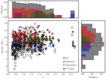
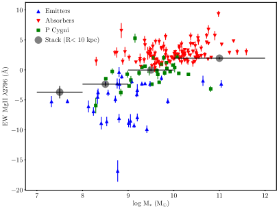
Figure 1: Left: The stellar mass as a function of redshift for all the galaxies (open black circle) in MAGG and MUDF with Mg ii coverage in the redshift range, $0.7\leq z\leq 2.3$. The galaxies with Mg ii detection in the 1D spectra are marked by upward blue triangles for Emitters, downward red triangles for Absorbers, and green squares for P Cygni profiles. The histograms of the stellar mass and redshift distributions are shown in the right and top panels, respectively. The dotted line marks the median property of the sample. The color scheme of the histograms and dotted lines is the same as that of the symbols. Right: The equivalent width of the Mg ii $\lambda$2796 line as a function of the stellar mass for the Emitters, Absorbers, and P Cygni sub-samples, following the same color scheme as in the left panel. The equivalent width estimates obtained from stacking the spectra of all galaxies (shown by open black circles in the left panel) in four different stellar mass bins, extracted within a central circular aperture of radius 10 kpc, are also shown in grey circles.

3 Radiative Transfer Modeling for Mg ii spectra

3.1 Spectral fitting pipeline

Table 3: Free parameters used in the Mg ii radiative transfer simulations. The total number of simulated spectra is 201,600.

Parameter	Range	Bins	Note
${N}_{\rm MgII}$	$10^{12.5}-10^{17}{\rm\,cm^{-2}}$	$0.5\,$dex	Mg ii column density
$v_{\rm exp}$	$-200-500{\rm\,km\,s^{-1}}$	$50{\rm\,km\,s^{-1}}$	expansion velocity
$\sigma_{\rm Ran}$	$25-200{\rm\,km\,s^{-1}}$	$25{\rm\,km\,s^{-1}}$	random speed of Mg ii medium
$\sigma_{\rm Src}$	$25-200{\rm\,km\,s^{-1}}$	$25{\rm\,km\,s^{-1}}$	width of intrinsic Mg ii emission
${\rm EW}_{\rm int}$	$0-20$ Å	1 Å	equivalent width of intrinsic Mg ii emission

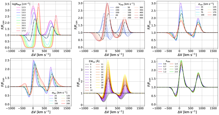
Figure 2: Simulated Mg ii doublet spectra as a function of the Doppler factor $\Delta$V from the line center of the Mg ii K line using the 3D Monte-Carlo radiative transfer simulation RT-scat. The black dashed, dotted line is the fiducial spectrum at ${N}_{\rm MgII}$ = $10^{14}{\rm\,cm^{-2}}$, $v_{\rm exp}$ = 200  km s^-1 , $\sigma_{\rm Ran}$ = 100  km s^-1 , $\sigma_{\rm Src}$ = 100  km s^-1 , ${\rm EW}_{\rm int}$ = 10 Å  and $z_{\rm obs}$ = 1. Each panel showcases the spectral behavior varying six parameters, ${N}_{\rm MgII}$, $v_{\rm exp}$, ${\rm EW}_{\rm int}$, $\sigma_{\rm Ran}$, $\sigma_{\rm Src}$, and $z_{\rm obs}$.

To analyze the observed Mg ii signal, we utilize the simulated spectra generated by the 3D Monte-Carlo simulation RT-scat (Chang et al., 2023; Chang & Gronke, 2024). Specifically, we adopt a spherical model composed of a spherical Mg ii halo with varying expanding velocity and a point source at the center of this spherical halo. We assume two types of intrinsic spectral distributions near the Mg ii doublet: a flat continuum, representing the stellar continuum near 2800 Å, and Gaussian-like emission with a fixed flux ratio of Mg ii $\lambda$2796 (K line) & $\lambda$2803 (H line) at 2 and width of $\sigma_{\rm Src}$. The outer radius of the halo, denoted as $R_{\rm H}$, is fixed at 100 kpc; the inner radius is 1 kpc, corresponding to $0.01R_{\rm H}$. This choice is made arbitrarily, but as the radiative transfer is affected by the intercepting column densities (and kinematics) and not by the physical distances, the solutions found here are generally valid and can be rescaled to any other halo radius. The radial velocity of the outflow is proportional to the radius from the central source, i.e., $v(r)={v_{\rm exp}}r/R_{\rm H}$. We generate 201,600 Mg ii spectra across a parameter range outlined in Table 3, considering five parameters:

• The Mg ii column density (${N}_{\rm MgII}$) measured from the center to $R_{\rm H}$. Specifically, we fill the spherical cold gas halo from the inner radius $0.01R_{\rm H}$ to the outer radius $R_{\rm H}$ with a constant Mg ii number density $n_{\text{Mg\,{ii}}}={{N}_{\rm MgII}}/0.99R_{\rm H}$.

• The maximum outflow velocity ($v_{\rm exp}$) reached the edge of the halo.

• The random motion of Mg ii parametrized by $\sigma_{\rm Ran}$. Note that we employ the ‘microturbulent approximation’ in this work (as done in many previous studies; e.g., Verhamme et al., 2006; Gronke et al., 2015; Seon & Kim, 2020), and thus a given random velocity corresponds to an effective temperature $T_{\rm eff}\approx 3000\sigma_{\rm ran}^{2}\,{\rm K\,s}^{2}{\rm km}^{-2}+10^{4}\,$K.

• The two parameters describing the intrinsic emission from the point source, namely the width of the intrinsic Mg ii line ($\sigma_{\rm Src}$) and the equivalent width of intrinsic emission (${\rm EW}_{\rm int}$).

In order to compare the observed and simulated spectra, we have to take into account that the emergent spectrum is spatially varying. To mimic the observations closely, we use the ‘core’ spectrum, that is, the observed spectrum within $10\,$kpc projected distance as our fiducial integrated spectrum and refer to it henceforward as the ‘simulated’ spectrum. When modeling the full spatially varying spectrum, we define which range of projected radii are being used. In addition, we adopt the spatial resolution of MUSE ($\approx 6$ kpc at $z\approx 1$) in the simulated spectra through 2D Gaussian convolution and the spectral resolution of MUSE as a function of wavelength.

To obtain the best fitting set of the five parameters listed in Table 3, we compare the observed and simulated spectra using a chi-square test in wavelength space. The details of the fitting method are described in Appendix A.

3.2 Impact of the individual parameters

In this section, we highlight the change in the individual parameters described above on the emergent spectrum. While this allows for a better understanding and interpretation of the modeling results, we want to note that degeneracies and additional dependencies do exist (which are captured by our fitting pipeline). A more detailed exploration of the parameter space as well as general Mg ii radiative transfer is presented in Chang & Gronke (2024).

Figure 2 shows the dependencies of the Mg ii spectra on various parameters. In the left top panel, as the Mg ii column density (${N}_{\rm MgII}$) increases, the absorption feature gets stronger. Particularly, the variation of a spectral profile is large at ${N}_{\rm MgII}$ = $10^{13.5-14.5}{\rm\,cm^{-2}}$, where the optical depth of Mg ii at the line center increases from $\sim 1$ to $\sim 10$. The regime for this large variation depends on other parameters, namely $\sigma_{\rm R}$ and $v_{\rm exp}$, which affect the optical depth of the Mg ii doublet. Higher $\sigma_{\rm R}$ and $v_{\rm exp}$ enhance the ${N}_{\rm MgII}$ range in ${{N}_{\rm MgII}}=10^{14-15}{\rm\,cm^{-2}}$.

In the central top panel of Figure 2, the expansion velocity ($v_{\rm exp}$) induces the broadening of the absorption feature due to the distribution of the radial velocity. Since the radial velocity is proportional to the distance from the central source, a higher $v_{\rm exp}$ causes a wider absorption in the velocity range from 0  km s^-1 to $-$$v_{\rm exp}$. The spectra with a positive and negative $v_{\rm exp}$, representing outflow and inflow, show a blue- and red-shifted absorption feature, respectively.

Concerning the random motion ($\sigma_{\rm R}$) and intrinsic emission width ($\sigma_{\rm Src}$) in the right top and left bottom panels of Figure 2, respectively, their influences are comparatively similar. Increasing these parameters results in a broader red peak since a higher $\sigma_{\rm Src}$ intrinsically enhances the width of emission features, and $\sigma_{\rm R}$ also causes the line broadening via scattering. Increasing the equivalent width of intrinsic emission (${\rm EW}_{\rm int}$) strengthens the emission features. In the bottom right panel of Figure 2, we examine the dependence on observed redshift $z_{\rm obs}$. As the MUSE spectral resolution increases with increasing wavelength, the spectrum for a higher $z_{\rm obs}$ is slightly narrower than that for a lower $z_{\rm obs}$.

In summary, while our modeling approach varies all parameters simultaneously and thus takes the full spectral shape into account, the most constraining parts are the absorption features for the scattering medium (i.e., ${N}_{\rm MgII}$, $v_{\rm exp}$ and $\sigma_{\rm R}$) and the emission part of the observed Mg ii spectra for the emission parameters ($\sigma_{\rm Src}$ and ${\rm EW}_{\rm int}$). In the following section, we interpret the stacked Mg ii data based on the spectral behaviors illustrated in Figure 2.

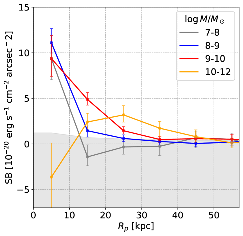
Figure 3: Azimuthally averaged surface brightness of the stacked Mg ii emission as a function of projected radius ${R}_{\rm p}$. The line colors represent the range of stellar mass bin of the stacked data, $\log{{M}_{\rm*}}/{{M}_{\odot}}$ = $7-8$ (green), $8-9$ (blue), $9-10$ (red), and $10-12$ (orange). The grey zone is the $3\sigma$ detection limit of the surface brightness as a function of ${R}_{\rm p}$.

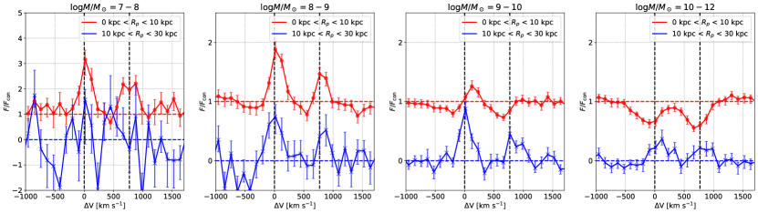
Figure 4: Stacked core spectrum in ${{R}_{\rm p}}<10\,\rm kpc$ (red), and stacked halo spectrum in ${R}_{\rm p}$ from 10 kpc to 30 kpc (blue), as a function Doppler factor $\Delta V$ of the Mg ii K line. Each panel represents different stellar mass bins, $\log{{M}_{\rm*}}/{{M}_{\odot}}$ = $7-8$, $8-9$, $9-10$, and $10-12$. The stacking halo spectra are continuum subtracted. The core and halo spectra are normalized by dividing by the continuum of the core spectrum for each mass bin. The red and blue dashed horizontal lines represent the normalized continuum and the subtracted continuum (i.e., $\sim 0$ $\rm erg\,s^{-1}\,cm^{-2}\,arcsec^{-2}$) near the Mg ii doublet, respectively. The black vertical lines represent the line center of the Mg ii K and H lines.

4 Dependence of Stacked Mg ii on Stellar Mass

In this section, we explore the dependence of the stacked Mg ii data on stellar mass. Figure 3 presents radial profiles of surface brightness (SB) for the Mg ii doublet for four distinct $\log{{M}_{\rm*}}/{{M}_{\odot}}$ bins: 7-8, 8-9, 9-10, and 10-12. The SB values are the azimuthally averaged values in circular annuli of radius 10 kpc from the galaxy centre. Here, negative and positive values of SB denote Mg ii absorption and emission features, respectively. The SB profiles are obtained from narrow-band images of the stacked Mg ii emission over the velocity range 0 to 300  km s^-1 around both the Mg ii K and H line centroids, after subtracting the continuum emission. As shown in Figure 1, when ${M}_{\rm*}$ increases, the spectrum shows stronger absorption features. Thus, in the core region at $R_{p}<10$ kpc, the SB for ${M}_{\rm*}$/${M}_{\odot}$ $=10^{10-12}$ is negative due to a strong absorption. However, in the halo region at $R_{p}>20\,\rm kpc$, the trend differs from that in the core region. In Figure 3, the SB profile becomes more extended with increasing ${M}_{\rm*}$. This is because Mg ii emission is spatially extended to the halo through scattering with Mg ii atoms in the cold medium surrounding a galaxy.

4.1 Mg ii Spectra in Core and Halo Regions

Figure 4 shows the core (projected radius, $R_{p}$ = 0-10 kpc) and halo ($R_{p}$ = 10-30 kpc) spectra for different stellar mass bins. Here, the $y$-axis is the observed flux divided by the continuum, $F/F_{\rm con}$. As also shown in Figure 3, the strength of the absorption feature increases with increasing ${M}_{\rm*}$. The core spectrum at ${M}_{\rm*}$/${M}_{\odot}$ $=10^{7-8}$ exhibits clear emission features, while the P-Cygni profile starts to appear at ${M}_{\rm*}$/${M}_{\odot}$ $=10^{8-9}$ and is prominent at ${M}_{\rm*}$/${M}_{\odot}$ $=10^{9-10}$. Notably, strong Mg ii absorption without any emission feature is evident at ${M}_{\rm*}$/${M}_{\odot}$ $=10^{10-12}$. Therefore, this trend shows that the rich cold gas within and around a massive galaxy causes a strong absorption feature of the Mg ii spectra within the galaxy.

The halo spectrum is intricately linked to the absorption in the core spectrum. In the left panel of Figure 4 for ${M}_{\rm*}$/${M}_{\odot}$ $\geq 10^{8}$, where core spectra exhibit significant absorption features, Mg ii emission becomes distinctly detectable in the halo. In the low ${M}_{\rm*}$ regime ($<10^{8}{{M}_{\odot}}$), the absorption (emission) feature of Mg ii is negligible in the core (halo) spectrum. This indicates a clear correlation between absorption in the core region and emission in the halo. For instance, in the case of optically thin cold gas for Mg ii (${N}_{\rm MgII}$ $<10^{13}{\rm\,cm^{-2}}$), Mg ii scattering effects are weak, resulting in an observed Mg ii emission profile without absorption features and a negligible emission in the halo. Conversely, in cases of optically thick cold gas for Mg ii (${N}_{\rm MgII}$ > $10^{14}{\rm\,cm^{-2}}$) surrounding galaxies, the gas in the observed direction and along its perpendicular direction causes absorption features in the core spectrum and emission features in the halo spectrum, respectively. Thus, abundant cold gas induces absorption in the core region and emission in the halo.

However, in the right panels of Figure 4, the halo spectrum at ${M}_{\rm*}$/${M}_{\odot}$ $=10^{9-10}$ is stronger than that at ${M}_{\rm*}$/${M}_{\odot}$ $=10^{10-12}$, although its absorption is weaker than that for the higher stellar mass. We expect that this originates from the dusty cold medium, angular distribution of cold gas around massive galaxies, or Mg ii emission spatially extended to a larger radius. We will investigate the weakening of the halo spectrum at the highest mass regime later in § 5.3 through the fitting results of the stacked spectra.

4.2 Characterization of Mg ii K and H Line Absorption

In general, when both the K and H lines at 2796 and 2803 Å, are not optically thick, the absorption of the K line is typically stronger than that of the H line due to the scattering cross section of the K line being twice as high. In a medium that is highly optically thick for both lines ($\tau_{0}\gg 1$), the absorption features become saturated, and both K and H lines exhibit similar absorption profiles. Thus, the K and H lines’ absorption strength ratio is always between 2 to 1.

However, in the right panels of Figure 4, the core spectra for ${{M}_{\rm*}}/{{M}_{\odot}}=10^{9-10}$ and $10^{10-12}$ show stronger absorption in the H line than in the K line. This serves as evidence of significant intrinsic Mg ii emission. If the Mg ii emission arises from recombination or collisional excitation, the Mg ii K line emission should be approximately twice as luminous as the H line emission. The brighter Mg ii K emission, when mixed with saturated absorption due to low spectral resolution or stacking process, can result in weaker absorption in the observed K line compared to the H line. For this reason, we expect that massive (${M}_{\rm*}$/${M}_{\odot}$ $>10^{9}$) galaxies exhibit both a strong stellar continuum and intrinsic Mg ii emission. We will discuss further details through our modeling in the following section.

5 Results

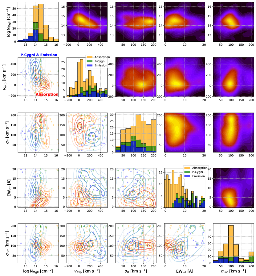
Figure 5: Histograms of fitting parameters, ${N}_{\rm MgII}$, $v_{\rm exp}$, $\sigma_{\rm R}$, ${\rm EW}_{\rm int}$, and $\sigma_{\rm Src}$. The panels along the diagonal show the stacked histograms of each parameter. The colors represent the type of spectrum: ‘Absorption’ (orange), ‘P-Cygni’ (green), and ‘Emission’ (blue). The panels in the lower triangle show the density map correlation between the two parameters.

This section analyzes the fitting results of the observed spectra, including individual detections and stacks. Figure 5 shows the histogram of and correlations between five fitting parameters: ${N}_{\rm MgII}$, $v_{\rm exp}$, $\sigma_{\rm R}$, ${\rm EW}_{\rm int}$, and $\sigma_{\rm Src}$. We explore the distribution of fitting parameters and their correlation through the fitting results of individual detections. Note that our pipeline manages to reproduce observed spectra very well. Examples of fitting individual detections, as well as a discussion of the fit quality, are presented in Appendix A.

From the panels in the upper triangle of Figure 5, there is a strong correlation only between the parameters, ${N}_{\rm MgII}$ and $v_{\rm exp}$. On the other hand, in the panels in the lower triangle of Figure 5, the correlations of the absorption spectra (red) and P-Cygni & emission spectra (blue) are separately distributed. This indicates that the type of the spectrum is crucial to understanding the physical mechanism giving rise to the Mg ii spectrum. Therefore, we compare the distributions of parameters for each spectral type: ‘Absorption’, ‘P-Cygni’, and ‘Emission’ as defined in § 2.

5.1 Analysis of Fitting Parameter Trends

The Mg ii column density, ${N}_{\rm MgII}$, is a prominent indicator of the strength of an absorption feature. The spectra at ${{N}_{\rm MgII}}<10^{14}{\rm\,cm^{-2}}$ have a negligible absorption feature as can be seen in the left top panel of Figure 2. In the first top panel of Figure 5, the distributions from ‘absorption’ (orange), ‘P-Cygni’ (green), and ‘emission’ (blue) spectra indicate that the behavior of simulated spectra for various ${N}_{\rm MgII}$ is well reflected. For the absorption and P-Cygni spectra where an absorption feature appears, ${N}_{\rm MgII}$ of the absorption cases cluster around $10^{14.5}{\rm\,cm^{-2}}$ and ${N}_{\rm MgII}$ for P-Cygni cases $\geq 10^{14}{\rm\,cm^{-2}}$. ${N}_{\rm MgII}$ of the emission spectra is skewed distribution toward a lower value in the vicinity of ${{N}_{\rm MgII}}\leq 10^{14}{\rm\,cm^{-2}}$. In addition, our modeling indicates that half of the emission cases have a negligible absorption feature at ${N}_{\rm MgII}$ < $10^{14}{\rm\,cm^{-2}}$. Consequently, ${N}_{\rm MgII}$ of absorption spectra is higher than that of emission spectra.

The expansion velocity, $v_{\rm exp}$, is estimated by the location of the dip in the Mg ii absorption profile and represents the kinematics of optically thick cold gas (${N}_{\rm MgII}$ $\geq 10^{14}{\rm\,cm^{-2}}$). In the second panel on the diagonal from the top-left to the bottom-right of Figure 5, the histogram of $v_{\rm exp}$ has two peaks at 0  km s^-1 and 200  km s^-1 . This indicates that Mg ii absorption originates from two types of cold gas: static, slow cold gas ($v_{\rm exp}$ $<100$  km s^-1 ) and outflowing galactic wind ($v_{\rm exp}$ $>200$  km s^-1 ). The absorption spectra dominate the primary peak at 0  km s^-1 and the inflow regime (i.e., negative $v_{\rm exp}$). Most galaxies with a high stellar mass (${M}_{\rm*}$/${M}_{\odot}$ $>10^{10}$) show Mg ii in absorption, as shown in Figure 1. Thus, the abundant static cold ISM or infalling gas of massive galaxies causes the absorption spectrum without an emission feature at ${{R}_{\rm p}}~<~10$ kpc.

The random motion of cold gas, $\sigma_{\rm R}$, represents the width of the absorption profile. In the third panel on the diagonal of Figure 5, $\sigma_{\rm R}$ of P-Cygni and emission spectra are broadly distributed from 0 to 200  km s^-1 . In the absorption case, $\sigma_{\rm R}$ is clustered towards higher values. These distributions indicate that static, slow cold gas (absorption spectra) has faster random motion than the outflowing gas (P-Cygni and emission spectra). But, in the second panel on the third row of Figure 5, P-Cygni and emission cases (blue triangles) show a positive correlation between $v_{\rm exp}$ and $\sigma_{\rm R}$.

The equivalent width of intrinsic Mg ii emission, ${\rm EW}_{\rm int}$, represents the strength of the Mg ii emission from the source. In the fourth panel on the diagonal of Figure 5, ${\rm EW}_{\rm int}$ of the absorption spectra are broadly distributed at ${\rm EW}_{\rm int}$ $<10$ Å. This is because the absorption-only spectrum can also indicate the presence of intrinsic emission, which is washed out by the absorption. Thus, the intrinsic emission can be estimated by comparing the absorption line ratio of K and H lines as discussed in § 4.2. Furthermore, the same panel shows that ${\rm EW}_{\rm int}$ of the P-Cygni and emission spectra are higher than 5 Å  to reproduce their emission features.

The fifth panel on the diagonal of Figure 5 shows that the width of the intrinsic emission, $\sigma_{\rm Src}$, of absorption spectra is clustered at 100  km s^-1 . However, measuring $\sigma_{\rm Src}$ from the absorption spectra is challenging because of the absence of a clear emission feature in the whole spectrum. Thus, it is hard to interpret the physical properties of the observed spectra from the $\sigma_{\rm Src}$ of the absorption spectra. $\sigma_{\rm Src}$ of P-Cygni spectra is higher than that of the emission spectra since a higher $\sigma_{\rm Src}$ enhances the red spectral peak, such as in outflowing gas, as shown in the left bottom panel of Figure 2.

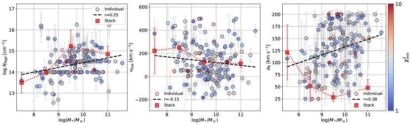
Figure 6: Fitting parameters characterizing the cold gas as a function of stellar mass ${M}_{\rm*}$: Mg ii column density ${N}_{\rm MgII}$ (left), expansion velocity $v_{\rm exp}$ (center), and the random motion of cold gas $\sigma_{\rm R}$ (right). The circle colors indicate the minimum $\chi^{2}$ value, with error bars showing $\pm$ weighted standard deviation (see § A). Red squares represent the fitting results for stacked spectra across four stellar mass bins: $\log M_{*}/M_{\odot}=7-8$, $8-9$, $9-10$, and $10-12$. The inclination of the black dashed lines represents the linear correlation between fitting parameters and $\log{{M}_{\rm*}}/{{M}_{\odot}}$. Pearson correlation coefficient $p$ for $\log{{N}_{\rm MgII}}$, $v_{\rm exp}$, and $\sigma_{\rm R}$ are 0.25, $-0.15$, and 0.38, respectively.

From the above results, it is clear that the distributions of the five parameters depend on the type of the observed Mg ii spectrum. Particularly, the distribution parameters of the absorption spectra are different from those of P-Cygni & emission spectra. The panels in the lower triangle of Figure 5 show separately distributed density maps for the correlations between two parameters of the absorption spectrum (red) and P-Cygni & emission spectra (blue). Compared with the P-Cygni & emission cases, the absorption cases have higher ${N}_{\rm MgII}$ and $\sigma_{\rm R}$, and lower $v_{\rm exp}$ and ${\rm EW}_{\rm int}$. This indicates that the absorption spectrum mainly originates from optically thick slow or inflowing cold gas with large random motion, and most P-Cygni and emission spectra come from the outflowing gas. As most high stellar mass galaxies exhibit Mg ii in absorption (see Figure 1), we will explore the relation between the fitting parameters and stellar mass in the following section.

5.2 Dependence of Fitting Parameters on Stellar Mass

5.2.1 Correlation between Stellar Mass and Cold Gas Properties

This section focuses on the correlation between the stellar mass, ${M}_{\rm*}$, and three critical parameters that characterize the cold gas: the Mg ii column density (${N}_{\rm MgII}$), the expansion velocity ($v_{\rm exp}$), and the random motion of the cold gas ($\sigma_{\rm R}$). Figure 6 shows weight averages of ${N}_{\rm MgII}$, $v_{\rm exp}$, and $\sigma_{\rm R}$, estimated from fitting with the simulated spectra as a function of stellar mass ${M}_{\rm*}$. The left panel of Figure 6 shows a positive correlation between ${N}_{\rm MgII}$ and ${M}_{\rm*}$ with Pearson correlation coefficient $p=0.25$. In the low ${M}_{\rm*}$ regime ($<10^{9}{{M}_{\odot}}$), ${N}_{\rm MgII}$ informed from stacked spectra (red squares) and most individual detections (circles) are less than $10^{14}{\rm\,cm^{-2}}$. In the high ${M}_{\rm*}$ regime ($>10^{9}{{M}_{\odot}}$), ${N}_{\rm MgII}$ values are higher than $10^{14}{\rm\,cm^{-2}}$. This trend suggests that the absorption features in the stacked spectrum become stronger with increasing ${M}_{\rm*}$, as shown in Figure 4. Furthermore, most of the individual detections in the high ${M}_{\rm*}$ regime are categorized by the absorption profile, as depicted in Figure 1.

In the center panel of Figure 6, $v_{\rm exp}$ and ${M}_{\rm*}$ show a negative correlation with $p=-0.15$. $v_{\rm exp}$ in the low ${M}_{\rm*}$ regime is largely scattered in $v_{\rm exp}$ from $-100$  km s^-1 to 500  km s^-1 . Note that the measurements of $v_{\rm exp}$ in this low mass regime are uncertain and have a large error bar because most individual detections are classified as emission in Figure 1. However, $v_{\rm exp}$ is predominantly distributed below $100{\rm\,km\,s^{-1}}$ in the high ${M}_{\rm*}$ regime. This pattern implies that such absorption could originate either from the cold ISM within galaxies or intrinsic Mg ii absorption in the stellar continuum. Consequently, the different $v_{\rm exp}$ distributions in the high and low mass regimes indicate that the kinematics of the optically thick cold gas traced by the Mg ii doublet depends on the stellar mass of the galaxies, as also shown by Figure 5.

The right panel of Figure 6 demonstrates that $\sigma_{\rm R}$ of individual detections increases with increasing ${M}_{\rm*}$. This trend is expected, as galaxies of higher stellar mass generally have more massive halos, which experience enhanced random motion of cold gas. However, the measurements of $\sigma_{\rm R}$ have large error bars. It is challenging estimating $\sigma_{\rm R}$ accurately when the spectral resolution (spectral resolution of MUSE spectra $\approx$ 85-200  km s^-1 at $z_{\rm obs}$ = 0.6 - 2.2, see Equation 1) is higher than $\sigma_{\rm R}$. In addition, as the stacking process leads to additional broadening and effectively lowers the resolution, the measurements of $\sigma_{\rm R}$ of stacking spectra are also inaccurate.

5.2.2 Intrinsic Mg ii emission

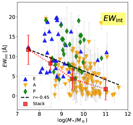
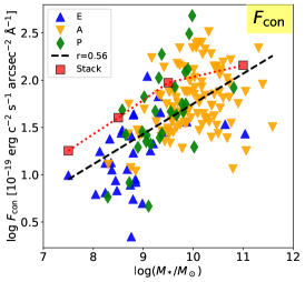
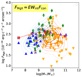
Figure 7: The equivalent width of intrinsic Mg ii emission ${\rm EW}_{\rm int}$ (left), the continuum flux near Mg ii emission $F_{\rm con}$ (center), and the flux of intrinsic Mg ii emission $F_{\rm MgII}$ (right) as functions of ${M}_{\rm*}$. The blue triangles, orange nablas, and green diamonds represent individual spectra classified as ’Emission,’ ’Absorption,’ and ’P-Cygni,’ respectively. The inclination of the black dashed lines represents values of $p$, which are 0.45 and 0.56 for ${\rm EW}_{\rm int}$ and $F_{\rm con}$, respectively.

Due to its resonant nature, the formation of the Mg ii line profile is determined by the properties of cold gas and intrinsic Mg ii emission. In the previous section, we explored the correlation between cold gas properties and the stellar mass of the galaxy. This section focuses on the intrinsic Mg ii emission parameters obtained through fitting of the emergent line shape. The findings from § 4.2 establish that spectra with K line (Mg ii $\lambda 2796$) absorption weaker than the H line (Mg ii $\lambda 2803$) distinctly suggest the existence of intrinsic Mg ii emission. Two of the fitting parameters, the equivalent width and the width of the intrinsic Mg ii emission, allow us to investigate the properties of the intrinsic emission.

Figure 7 shows the fitting results for the equivalent width of intrinsic Mg ii emission, ${\rm EW}_{\rm int}$, the stellar continuum near Mg ii emission, $F_{\rm con}$, and the flux of intrinsic Mg ii emission, $F_{\rm MgII}$, as a function of ${M}_{\rm*}$. In the left panel of Figure 7, ${\rm EW}_{\rm int}$ of individual detections and stacked spectra shows a negative correlation (see the black dashed line). It is because ${\rm EW}_{\rm int}$ of most individual cases in the high mass regime (${M}_{\rm*}$ $>10^{9}{{M}_{\odot}}$) are less than 5 Å. However, the trend of ${\rm EW}_{\rm int}$ is insufficient to conclude that Mg ii emission intrinsically decreases with increasing ${M}_{\rm*}$ since, in general, more massive galaxies generate more Mg ii photons.

To measure the total flux of the intrinsic Mg ii emission, the continuum flux $F_{\rm con}$ is multiplied by ${\rm EW}_{\rm int}$. The center panel of Figure 7 shows that $F_{\rm con}$ increases as ${M}_{\rm*}$ increases. In the right panel of Figure 7, we calculate the intrinsic Mg ii emission flux as $F_{\rm MgII}={{\rm EW}_{\rm int}}F_{\rm con}$. The $F_{\rm MgII}$ of individual detections are largely scattered across ${M}_{\rm*}$ since ${\rm EW}_{\rm int}$ and $F_{\rm con}$ show a positive and negative correlation with ${M}_{\rm*}$, respectively. In addition, the trend of $F_{\rm MgII}$ with ${M}_{\rm*}$ is not monotonic. The $F_{\rm MgII}$ of stacked spectra increases with increasing ${M}_{\rm*}$ until ${M}_{\rm*}$/${M}_{\odot}$ $<10^{10}$ and decreases at ${M}_{\rm*}$/${M}_{\odot}$ $=10^{10-12}$.

To explore the trend of intrinsic Mg ii emission $F_{\rm MgII}$, we separately checked the $F_{\rm MgII}$ distribution of ’absorption’ and ’emission’ & ’P-Cygni’ spectra. The right panel of Figure 7 shows the contour of the two distributions. The ’emission’ & ’P-Cygni’ detections positively correlate with ${M}_{\rm*}$ (see the blue contours). The ’absorption’ cases (the red contours) show a negative correlation with ${M}_{\rm*}$. The strength of intrinsic Mg ii emission increases with increasing ${M}_{\rm*}$ over ${{M}_{\rm*}}/{{M}_{\odot}}=10^{7-9}$. However, it decreases at ${{M}_{\rm*}}/{{M}_{\odot}}>10^{10}$ because abundant dusty cold gas within galaxies causes a weaker continuum and stronger intrinsic absorption. In addition, we expect some of the large scatter in the distribution of $F_{\rm MgII}$ to originate from line-of-sight effects because the dust extinction of the radiation near Mg ii emission along the edge-on direction of galaxies is higher than that along the face-on direction.

5.3 Modeling Halo Spectra and Surface Brightness Profiles

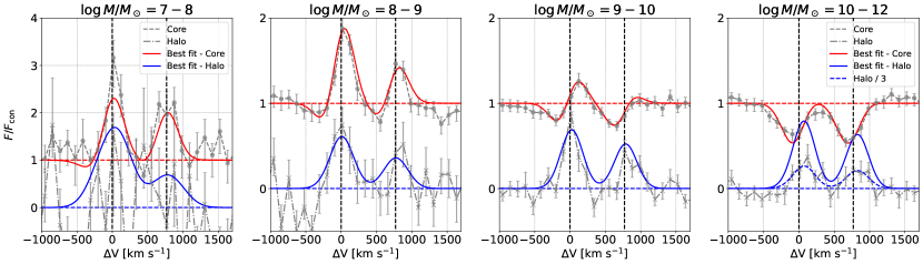
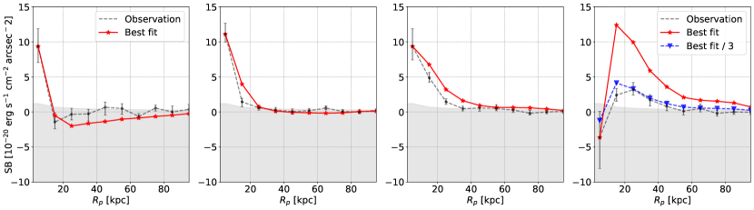
Figure 8: This figure presents the fitting of stacked spectra (top) and surface brightness (bottom) for four distinct stellar mass bins: $\log{{M}_{\rm*}}/{{M}_{\odot}}=7-8$ (first), 8-9 (second), 9-10 (third), and 10-12 (fourth). In the top panels, gray dashed and dot-dashed lines denote the stacked spectra in the core (${R}_{\rm p}$ < 10 kpc) and halo (${R}_{\rm p}$ = $10-30$ kpc) regions, respectively, corresponding to the spectra in Figure 4. The red solid lines illustrate the best-fit simulated spectra with the minimum $\chi^{2}$, based on the core spectrum analysis. The blue dashed lines represent the halo spectrum from the best model for the core spectrum. In the bottom panels, the black dashed lines denoted the stacked surface brightness, corresponding to those in Figure 3. The red solid line illustrated the best-fit surface brightness from the best model for the core spectrum. For lower mass ranges ($\log{{M}_{\rm*}}/{{M}_{\odot}}<9$), depicted in the top left panels, the simulated halo spectra align closely with the observed spectra. Conversely, in the right panel for the highest mass range ($\log{{M}_{\rm*}}/{{M}_{\odot}}=10-12$), the simulated spectrum significantly overestimates the observed halo emission. The surface brightness of the best fit divided by three (blue dashed) is similar to the observed one.

The resonant nature of the Mg ii doublet photons allows for interactions with cold gas across a wide range of conditions, provided the Mg ii column density (${N}_{\rm MgII}$) exceeds $10^{13}{\rm\,cm^{-2}}$, as shown in Figure 2. These interactions result in Mg ii absorption features from cold gas within star-forming regions or the ISM, P-Cygni profiles from Mg ii scattering in outflowing gas, and spatially extended Mg ii emission due to scattering of the gas in the outskirts of galaxies. Given that Mg ii spectra from galaxies are often observed with the stellar continuum, the resultant spectral profiles encapsulate these phenomena alongside inherent Mg ii absorption within the stellar continuum. Nonetheless, modeling based only on the core spectrum (${{R}_{\rm p}}<10$ kpc) is insufficient to disentangle the various mechanisms contributing to the Mg ii line formation. This is in the case of galaxies with ${M}_{\rm*}$/${M}_{\odot}$ $>10^{10}$, where the fitted expansion velocities $v_{\rm exp}$, predominantly cluster around $0{\rm\,km\,s^{-1}}$, indicating absorption features concentrated near the line center in this mass range, as shown in Figure 5. This scenario complicates the differentiation of Mg ii absorption attributable to either the gas within or around galaxies. This section extends the investigation to stacked spectra within the halo region (${{R}_{\rm p}}=10-30$ kpc), aiming to clarify these distinctions.

Table 4: Fitting parameters through the radiative transfer modeling of stacked spectra in the core region at ${{R}_{\rm p}}<10\,\rm kpc$ for four stellar mass bins.

${{M}_{\rm*}}/{{M}_{\odot}}$		$\log{{N}_{\rm MgII}}$ [ cm-2 ]	$v_{\rm exp}$ [ km s-1 ]	$\sigma_{\rm Ran}$ [ km s-1 ]	$\sigma_{\rm Src}$ [ km s-1 ]	${\rm EW}_{\rm int}$ [Å]
$10^{7-8}$	Average‡	13.5	222	121	39	11.7
	$\sigma^{*}$	0.49	197	57	19	3.7
	Best†	14	200	200	25	20
$10^{8-9}$	Average‡	14.0	250	52	31	8.2
	$\sigma^{*}$	0.12	51	32	11	1.6
	Best†	14	250	25	25	7
$10^{9-10}$	Average‡	15.2	120	28	46	4.3
	$\sigma^{*}$	0.77	28	8.3	23	2.6
	Best†	14.5	150	25	50	4
$10^{10-12}$	Average‡	14.8	112	48	81	1.7
	$\sigma^{*}$	0.39	35	17	54	2.8
	Best†	15	100	50	25	2

${\ddagger}$: Weighted average in Eq. 3, $*$: Weighted standard deviation in Eq. 4. ${\dagger}$: parameters of best-fit model with minimum $\chi^{2}$ in Eq. 2,

Figure 8 shows the stacked spectra in both core and halo regions, as well as the SB profiles with the best-fit models with a minimum $\chi^{2}_{\nu}$value for different mass bins. The best-fit parameters are shown in Table 4. We found the best fit using the observed spectrum in the core region at ${{R}_{\rm p}}<10$ kpc. The best fits for the halo spectrum and the SB profiles are those of the model with parameters estimated by fitting the spectrum in the core region. It can be seen from the top panels that the best-fit spectra are well-matched with the observed ones in the core region. For low-mass galaxies (${M}_{\rm*}$/${M}_{\odot}$ $<10^{9}$), the halo spectra and SB profiles from the best-fit model closely match the observations. However, for higher masses (${M}_{\rm*}$/${M}_{\odot}$ $>10^{9}$), the model predicts stronger halo spectra and higher SB profiles compared to observations, with this discrepancy becoming especially pronounced for ${M}_{\rm*}$/${M}_{\odot}$ $>10^{10-12}$.

The notable differences observed in the halo region for galaxies with ${M}_{\rm*}$/${M}_{\odot}$ $>10^{10-12}$ indicate that intrinsic Mg ii absorption in massive galaxies significantly affects Mg ii emission in their outskirts. Additionally, anisotropic distributions of cold Mg ii gas (e.g. Guo et al., 2023; Pessa et al., 2024) can affect the observed halo emission. In the right top panel of Figure 8, we illustrate the modified halo spectrum, which represents the original best fit reduced by a factor of three. Using this scaled model, we also recalculated the SB profile, which now closely matches the observed profiles. Therefore, we conclude that intrinsic absorption, anisotropic gas distribution, and dust in CGM significantly weaken the halo emission, reducing it by up to 50%.

5.4 Impact of Asymmetric Gas Distribution and Intrinsic Absorption on Surface Brightness Profiles

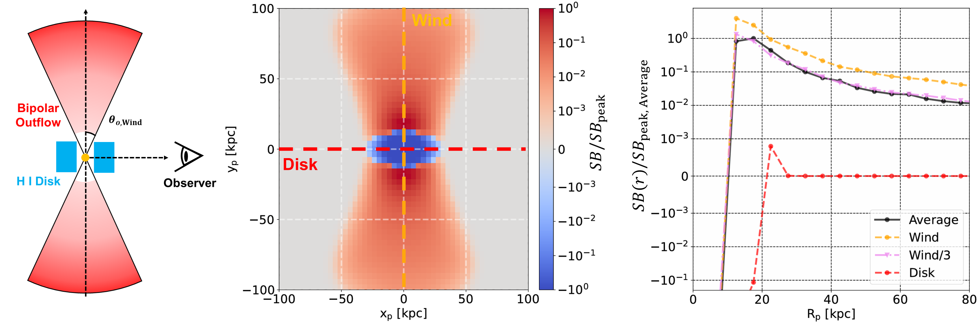
Figure 9: Mg ii surface brightness (SB) map and profiles for the bipolar wind model. Left: Schematic illustration of the bipolar wind model, including a central point source (orange), bipolar outflows (red), and a static H i disk (blue). The line of sight is perpendicular to the bipolar wind, viewed edge-on. Center: Simulated Mg ii SB map with a spatial resolution of $\sim 6$ kpc. Red indicates Mg ii emission, while blue shows absorption. Right: Mg ii SB profiles as a function of projected radius ${R}_{\rm p}$. The orange and red dashed lines represent profiles along the ‘Wind’ and ‘Disk’ directions, respectively, as shown in the center panel. The black solid line is the azimuthally averaged profile (corresponding to an observed ‘stacked’ profile), which closely matches the ‘Wind’ direction profile divided by three (violet dashed line), indicating that asymmetric gas distribution reduces the overall SB.

In this section, we explore the impact of asymmetric cold gas distribution and intrinsic absorption on the Mg ii surface brightness (SB) profile. Figure 9 illustrates the schematic of the asymmetric wind model and its SB profiles. The wind model consists of a central point source, a bipolar outflow for asymmetric gas distribution, and a static inner H i disk for intrinsic Mg ii absorption. The outflow is characterized by an opening angle $\theta_{\rm o,Wind}$, sharing the same kinematics and gas distribution as the spherical geometry described in § 3. These configurations allow us to assess how cold gas distribution influences the observed Mg ii emission. We use the best-fit parameters for the stacked spectrum with ${M}_{\rm*}$/${M}_{\odot}$ $>10^{10-12}$ from Table 4. The H i disk has an Mg ii column density of $10^{15}{\rm\,cm^{-2}}$ along the equatorial direction, with fixed random motion and temperature at 100  km s^-1 and $10^{4}\,\rm K$, respectively. The height and radius of the disk are 1 kpc and 5 kpc, respectively. We generate $10^{8}$ photons using a flat continuum with intrinsic Mg ii emission (${\rm EW}_{\rm int}$ = 2 Å) and collect photons, assuming the line of sight is perpendicular to the outflow direction.

The center panel of Figure 9 shows the simulated SB map. The Mg ii feature appears as absorption at the center due to the optically thick HI disk, while emission is visible in the extended halo due to scattering within the wind. These combined absorption and emission features resemble the observed stacked spectra with ${M}_{\rm*}$/${M}_{\odot}$ $>10^{10-12}$, as shown in the right panel of Figure 8, and also reported in other studies (Guo et al., 2023).

The right panel of Figure 9 compares the SB profiles along the wind (orange) and disk (red) directions. The wind profile is significantly more extended than that of the disk, indicating a directional influence of gas distribution. Naturally, for the stacked SB maps used here that do not take into account the orientation of the disk due to lack of high spatial resolution imaging, the averaged SB profile reflects the combined effect of different azimuthal angles. The average profile (black) in the right panel of Figure 9 matches the ‘Wind’ direction profile when reduced by a factor of three, highlighting that asymmetric gas distributions can significantly suppress the overall SB. As the opening angle decreases, this suppression factor increases, suggesting that the shape and directionality of the gas play a critical role in the observed emission.

Specifically, as demonstrated, the choice of $\theta_{\rm 0,wind}=30^{\circ}$ yields a suppression by a factor of $\sim 3$ – just as observed (cf. § 5.3). Thus, the inclusion of effects due to asymmetric gas distributions represents an alternative, elegant explanation to dust for the lower SB observed. However, in order to fully compare to the observed stacked data set, we would need to loosen the assumption of the wind being orthogonal to the line-of-sight as done (implicitly) here. We will explore this in future work.

6 Conclusions

In this study, we explored the properties of cold gas in and around galaxies at $z\sim 1$ by analyzing Mg ii spectra through radiative transfer modeling and data stacking techniques. Using a comprehensive sample of 624 galaxies from the MUSE Analysis of Gas around Galaxies (MAGG) and the MUSE Ultra Deep Field (MUDF) programs, we focused on both core (0-10 kpc) and halo (10-30 kpc) regions to gain insights into the distribution and kinematics of cold gas. We successfully modeled 167 individual detections and four stacked datasets for different stellar mass bins, as well as Mg ii emission extending beyond 10 kpc.

To do so, we assembled a suite of $>200,000$ radiative transfer models spanning the five-dimensional parameter space. Our main findings are as follows.

• In spite of the simplicity of the model, we could reproduce complex observed Mg ii spectra as well as surface brightness profiles. Specifically, only 3% (5/167) of individual detections result in chi-square values $\chi^{2}$, higher than 10 (Appendix A).

• Our analysis of stacked Mg ii spectra for different stellar mass bins revealed significant variations in spectral profiles and surface brightness with stellar mass (§ 4). In galaxies with lower stellar masses (${M}_{\rm*}$/${M}_{\odot}$ $<10^{9}$), Mg ii emission was observed in both the core (${R}_{\rm p}$ $<10$ kpc) and halo regions (10 kpc $<{{R}_{\rm p}}<30$ kpc). Conversely, in higher mass galaxies (${M}_{\rm*}$/${M}_{\odot}$ $>10^{10}$), strong absorption features dominated in the core, while the Mg ii surface brightness was more extended. This trend indicates that more massive galaxies have abundant cold CGM, leading to mass-dependent variations in cold gas distribution.

• Radiative transfer modeling allowed us to explore the relationships among key fitting parameters, such as the Mg II column density ${N}_{\rm MgII}$ and expansion velocity $v_{\rm exp}$ (Figure 5 in § 5.1). We found a negative correlation between ${N}_{\rm MgII}$ and $v_{\rm exp}$, indicating that regions with higher column densities tend to contain slower-moving gas. The expansion velocity was generally found to cluster around zero and 200  km s^-1 , suggesting the coexistence of static or slowly moving gas and outflows. Moreover, these parameters varied depending on the spectral type—‘Absorption,’ ‘P-Cygni,’ and ‘Emission’—revealing different physical conditions of the cold gas. Notably, higher stellar mass galaxies exhibited higher ${N}_{\rm MgII}$ and lower $v_{\rm exp}$ values, indicating an abundance of slowly moving cold gas in massive galaxies.

• The stacking analysis allowed us to access and model not only the core but also the halo spectra, thus allowing us to directly constrain the physical conditions of the CGM through emission (§ 5.3). By capturing simulated photon packages escaping in different projected radii bins, we could fit the stacked ‘core’ and ‘halo’ spectrum simultaneously. While the overall fit of both spectra is very good, we overproduce the ‘halo’ spectrum of the highest mass bin (${{M}_{\rm*}}/{{M}_{\odot}}>10^{10}$) by a factor $\sim 3$.

• Asymmetric gas distribution significantly reduces the stacked Mg ii surface brightness, with directional gas flows leading to notable variations in observed profiles (§ 5.4). This finding highlights the importance of accounting for anisotropic gas when interpreting extended Mg ii emission, particularly in the CGM of massive galaxies.

Interpreting observations of resonant lines such as Mg ii are notoriously complex due to the non-linear radiative transfer effects shaping the emergent observables. However, this process also holds the potential to probe the non-intrinsically emitting gas found, for instance, in the outskirts of galaxies. Advances in theoretical insight and computing power allow us to fit complex, observed spectra using full radiative transfer models and, thus, to obtain physical insights from resonant lines. In this work, we showed that it is possible to successfully reproduce a large number of observed spectra using this approach and obtain physical interpretable parameters. We furthermore correlate these parameters with galactic properties such as the stellar mass, and reveal several (anti-)correlations between them.

As several additional parameters, such as the asymmetric gas distribution, the dust content or related to the multiphase nature of the scattering medium, are not captured in our fitting pipeline, we see this effort as a first step in an ongoing process and plan to revisit this problem to better address the growing amount of resonant emission line data available.

Data Availability

Data related to this work will be shared on reasonable request to the corresponding author. The MUSE data used in this work are available from the European Southern Observatory archive (https://archive.eso.org).

Appendix A Deatils of the Mg ii spectral fitting pipeline

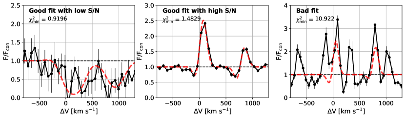
Figure 10: Best fitting results of three individual spectra. The left and center panels show ’good’ fit examples of spectra with low and high S/N, respectively. The right panel shows a ’bad’ fit example for $\chi_{\rm min}>10$. The black and red lines represent the observed and simulated spectra at the minimum $\chi^{2}$.

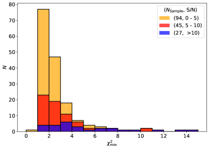
Figure 11: $\chi^{2}_{\rm min}$ histogram of individual detections. Colors represent the range of Mg ii signal-to-noise, 0-5 (orange), 5-10 (red), > 10 (blue).

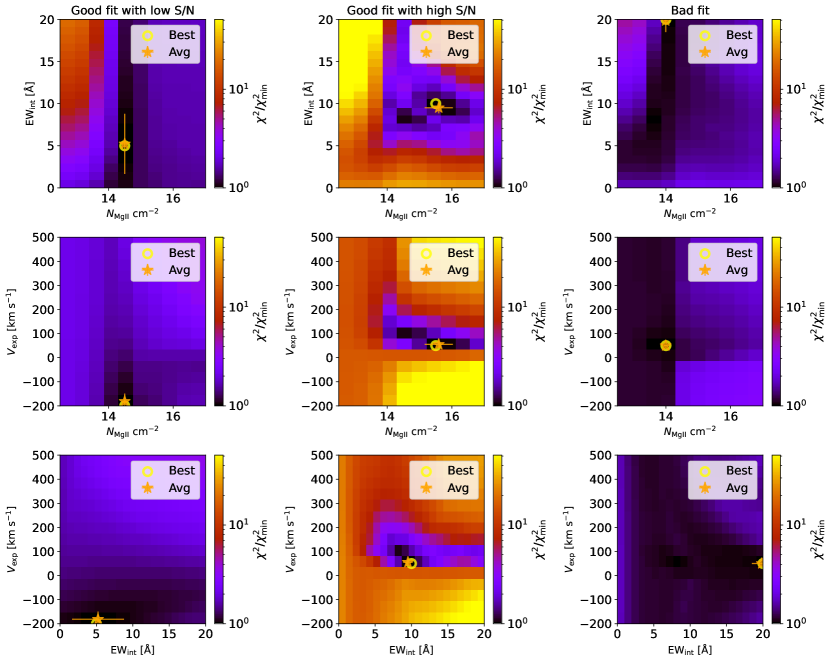
Figure 12: $\chi^{2}$ maps in ${\rm EW}_{\rm int}$- $v_{\rm exp}$ (top) and ${\rm EW}_{\rm int}$- ${N}_{\rm HI}$ (bottom) planes of three spectra in Figure 10. Each $\chi^{2}$ value is the minimum as two parameters in the $x-y$ axis are fixed. The yellow star marks represent the parameters of the best fit at the minimum $\chi^{2}$. The red open circles represent the values of the weighted average in Eq. 3 with the error bar corresponding to the weighted standard deviations in Eq. 4.

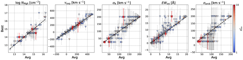
Figure 13: Comparisions of the parameters, ${N}_{\rm HI}$, $v_{\rm exp}$, $\sigma_{\rm R}$, ${\rm EW}_{\rm int}$, $\sigma_{\rm Src}$ between the weighted average and the best fit, which are $x$ and $y$ axes, respectively. The blue circles and inverse triangles represent individual spectra classified as ’emission’ & ’P-Cygni’ and ’absorption,’ respectively, as shown in Figure 1. The black dashed line is the $x=y$ graph. The error bar means the weighted standard division. Most individual and stacking spectra show similar weighted averages and best fit parameters.

This section describes how we analyze and fit the observed Mg ii spectra using simulated spectra to discern the scattering signature within the cold medium. We use a chi-squared test to fit the observed spectra with the simulated counterparts. For a comparative analysis of the two spectra, we collect the simulated spectrum in a radius of 0 to 10 kpc as Mg ii spectra of individual objects are observed in this radius range. We also adopt the typical MUSE spatial resolution of $\sim 6$ kpc at $z\approx 1$ through 2D Gaussian convolutions. Furthermore, we consider the observed spectral resolution. Because the spectral resolution of MUSE varies as a function of wavelength (Weilbacher et al., 2020), the spectral resolution variation must be considered to compare the observed and simulated spectra. The MUSE spectral resolution can be reproduced using the below relation:

$$R(\lambda)=p_{0}+p_{1}\lambda p_{2}\lambda^{2}+p_{3}\lambda^{3},$$ (1)

where $p_{0}=499.446$, $p_{1}=-0.201608$, $p_{2}=1.3029\times 10^{-4}$, and $p_{3}=7.87479\times 10^{-9}$, and $\lambda$ is in units of Å. In the fitting process, the spectral resolution $R_{\rm obs}$ is $\sim R(\lambda=({z_{\rm obs}}+1)\times 2800\textup{~\AA})$ as the wavelength of Mg ii doublet is in the rest frame $\sim 2800$ Å. We convolve the simulated spectra with the Gaussian function at the width $\sim 2.355R_{\rm obs}$ as $R(\lambda)$ represents the full-width half maximum of the spectral resolution. In the $z_{\rm obs}$ range of our samples (from 0.6 to 2.2), the spectral resolution is $1500-3500$, corresponding to the Gaussian width of 35-85  km s^-1 ; $R(\lambda)$ increases with increasing $z_{\rm obs}$. Note that $R=1000$, which is half of the average spectral resolution, is adopted to compare the simulated spectra with the stacked spectra, as the stacking process can lead to broadening of the line due to uncertainty in the redshifts, thus effectively degrading the resolution. After that, we normalize the observed spectrum by dividing it by the continuum level, which is obtained by averaging the spectrum near $-1500$  km s^-1 from Mg ii $\lambda$2796. The normalized flux of the continuum is fixed at 1 like in the simulated spectra in Figure 2. Also, the observed wavelength is converted to the wavelength in the rest frame by dividing by (1+$z_{\rm obs}$).

Given that the normalized observed spectrum and the mock simulated spectrum are $f_{\rm sim}$ and $f_{\rm obs}$, we estimate the chi-square value $\chi^{2}$ given by

$$\chi^{2}={{\sum^{N_{\rm obs}}_{i}\frac{({f_{\rm obs}}(\lambda_{i})-{f_{\rm sim}}(\lambda_{i}))^{2}}{\sigma_{\rm obs}^{2}(\lambda_{i})}}/{N_{\rm obs}}},$$ (2)

where $\lambda_{i}$ is the wavelength in the rest frame and $\sigma_{\rm obs}$ is the error of the observed spectrum. $N_{\rm obs}$ is the number of data points of the observed spectra in the wavelength range from 2788 Å to 2808 Å  which is the selected velocity range, from $-800$ to $+1300$  km s^-1 relative to Mg ii $\lambda$2796, capturing relevant features for our analysis. We estimate $\chi^{2}$ values of all simulated Mg ii spectra. Consequently, the simulated spectrum is defined as the best fit when the chi-square value $\chi^{2}$ is minimized, providing an optimal representation of the observed spectra through our fitting process.

The minimum chi-square value $\chi^{2}_{\rm min}$ depends on the signal-to-noise of Mg ii $S/N$. Figure 10 shows fitting examples for various $\chi^{2}_{\rm min}$. In the left and center panels of Figure 10, we show examples of two cases with low S/N ($\sim 2$) and high S/N ($\sim 17$), respectively. The fitting quality in the center panel is better than that in the left panel, although its $\chi^{2}_{\rm min}\sim 0.9$ is higher than in the left panel, $\sim 1.5$.

The best fit is not always similar to an observed spectrum. We show an example in the right panel of Figure 10, where the simulated spectrum does not match the observed spectrum because of multiple emission peaks ($\chi^{2}_{\rm min}>10$). Figure 11 shows the histogram of the minimum chi-square values $\chi^{2}_{\rm min}$ for various signal-to-noise $S/N$. The $\chi^{2}_{\rm min}$ of only five fit is higher than 10.

Figure 12 displays the $\chi^{2}$ maps of three spectra from Figure 10. These maps are presented in the ${{N}_{\rm MgII}}-{{\rm EW}_{\rm int}}$, ${{N}_{\rm MgII}}-{v_{\rm exp}}$, and ${{\rm EW}_{\rm int}}-{v_{\rm exp}}$ planes. In the top central panel of Figure 12, values of the lower ${N}_{\rm MgII}$ and ${\rm EW}_{\rm int}$ cases are comparable to the minimum. This local minimum region causes a degeneracy in the fitting results. For example, if both ${N}_{\rm MgII}$ and ${\rm EW}_{\rm int}$ increase in the best-fit model, a higher ${N}_{\rm MgII}$ suppresses Mg ii emission feature and a higher ${\rm EW}_{\rm int}$ enhances the feature conversely (see Figure 2). In this case, the simulated spectrum with higher ${N}_{\rm MgII}$ and ${\rm EW}_{\rm int}$ becomes similar to the best fit due to the opposite influence of the two parameters.

To avoid these degeneracies, we compute the weighted average of each simulated parameter. The weighted average of ${N}_{\rm MgII}$ is given by

$$\langle{{N}_{\rm MgII}}\rangle=\sum^{N_{\rm Sim}}_{j}N_{\rm MgII,j}\exp\left(-N_{\rm obs}\frac{\chi_{j}^{2}}{2}\right),$$ (3)

where $N_{\rm Sim}$ is the number of simulated spectra (201,600). Each simulated spectrum has a corresponding $\chi^{2}$ value denoted as $\chi_{j}^{2}$. Furthermore, the weighted standard deviation of ${N}_{\rm MgII}$

$$\sigma_{{N}_{\rm MgII}}=\langle{{N}_{\rm MgII}}^{2}\rangle-\langle{{N}_{\rm MgII}}\rangle^{2},$$ (4)

where $\langle{{N}_{\rm MgII}}^{2}\rangle$ is the weighted average of ${{N}_{\rm MgII}}^{2}$. In Figure 12, the orange star marks for the weighted average exist near points of the yellow open circle for the best-fit parameter.

To check the correlation between parameters of best fit and weighted average, we compare two values in Figure 13. Apart from a few objects, the two values are in a strong linear correlation $y=x$ in most individual spectra. In the fourth and fifth panels, some objects have large error bars (the weighted standard deviation) because these objects do not have enough emission to measure ${\rm EW}_{\rm int}$ and $\sigma_{\rm Src}$; the large error bar is along the ${\rm EW}_{\rm int}$ axis in the left panels of Figure 12.

In summary, we fit the observed Mg ii spectra using simulated spectra generated by RT-scat. We estimate the $\chi^{2}$ values using 201,600 simulated spectra and select as the best-fit model the one where $\chi^{2}$ is minimum. After that, we calculate the weighted average and standard deviation for each parameter to avoid fitting degeneracies. As a result, we set the fitting parameters as the weighted average and explore the trends of these parameters.

References

- Arrigoni Battaia et al. (2015) Arrigoni Battaia F., Hennawi J. F., Prochaska J. X., Cantalupo S., 2015, ApJ, 809, 163
- Arrigoni Battaia et al. (2019) Arrigoni Battaia F., Hennawi J. F., Prochaska J. X., Oñorbe J., Farina E. P., Cantalupo S., Lusso E., 2019, MNRAS, 482, 3162
- Bacon et al. (2010) Bacon R., et al., 2010, in McLean I. S., Ramsay S. K., Takami H., eds, Society of Photo-Optical Instrumentation Engineers (SPIE) Conference Series Vol. 7735, Ground-based and Airborne Instrumentation for Astronomy III. p. 773508, doi:10.1117/12.856027
- Bouché et al. (2016) Bouché N., et al., 2016, ApJ, 820, 121
- Burchett et al. (2021) Burchett J. N., Rubin K. H. R., Prochaska J. X., Coil A. L., Vaught R. R., Hennawi J. F., 2021, ApJ, 909, 151
- Carr et al. (2024) Carr C. A., et al., 2024, arXiv e-prints, p. arXiv:2409.05180
- Chang & Gronke (2024) Chang S.-J., Gronke M., 2024, MNRAS, 532, 3526
- Chang et al. (2023) Chang S.-J., Yang Y., Seon K.-I., Zabludoff A., Lee H.-W., 2023, ApJ, 945, 100
- Chen et al. (2020) Chen Y., et al., 2020, MNRAS, 499, 1721
- Chisholm et al. (2020) Chisholm J., Prochaska J. X., Schaerer D., Gazagnes S., Henry A., 2020, MNRAS, 498, 2554
- Crighton et al. (2015) Crighton N. H. M., Hennawi J. F., Simcoe R. A., Cooksey K. L., Murphy M. T., Fumagalli M., Prochaska J. X., Shanks T., 2015, MNRAS, 446, 18
- Dijkstra et al. (2019) Dijkstra M., Prochaska J. X., Ouchi M., Hayes M., eds, 2019, Lyman-alpha as an Astrophysical and Cosmological Tool Saas-Fee Advanced Course Vol. 46, doi:10.1007/978-3-662-59623-4_1.
- Dutta et al. (2020) Dutta R., et al., 2020, MNRAS, 499, 5022
- Dutta et al. (2021) Dutta R., et al., 2021, MNRAS, 508, 4573
- Dutta et al. (2023) Dutta R., et al., 2023, MNRAS, 522, 535
- Dutta et al. (2024) Dutta R., et al., 2024, arXiv e-prints, p. arXiv:2409.02182
- Faucher-Giguère & Oh (2023) Faucher-Giguère C.-A., Oh S. P., 2023, ARA&A, 61, 131
- Feltre et al. (2018) Feltre A., et al., 2018, A&A, 617, A62
- Fossati et al. (2018) Fossati M., et al., 2018, A&A, 614, A57
- Fossati et al. (2019) Fossati M., et al., 2019, MNRAS, 490, 1451
- Fossati et al. (2021) Fossati M., et al., 2021, MNRAS, 503, 3044
- Galbiati et al. (2023) Galbiati M., Fumagalli M., Fossati M., Lofthouse E. K., Dutta R., Prochaska J. X., Murphy M. T., Cantalupo S., 2023, arXiv e-prints, p. arXiv:2302.00021
- González Lobos et al. (2023) González Lobos V., et al., 2023, A&A, 679, A41
- Gronke et al. (2015) Gronke M., Bull P., Dijkstra M., 2015, ApJ, 812, 123
- Guo et al. (2023) Guo Y., et al., 2023, Nature, 624, 53
- Guo et al. (2024) Guo Y., et al., 2024, A&A, 691, A66
- Hennawi & Prochaska (2013) Hennawi J. F., Prochaska J. X., 2013, ApJ, 766, 58
- Henry et al. (2018) Henry A., Berg D. A., Scarlata C., Verhamme A., Erb D., 2018, ApJ, 855, 96
- Izotov et al. (2022) Izotov Y. I., Chisholm J., Worseck G., Guseva N. G., Schaerer D., Prochaska J. X., 2022, MNRAS, 515, 2864
- Katz et al. (2022) Katz H., et al., 2022, MNRAS, 515, 4265
- Leclercq et al. (2022) Leclercq F., et al., 2022, A&A, 663, A11
- Li et al. (2024) Li Z., et al., 2024, arXiv e-prints, p. arXiv:2410.11152
- Lofthouse et al. (2020) Lofthouse E. K., et al., 2020, MNRAS, 491, 2057
- Lofthouse et al. (2023) Lofthouse E. K., et al., 2023, MNRAS, 518, 305
- Lusso et al. (2019) Lusso E., et al., 2019, MNRAS, 485, L62
- Ouchi et al. (2020) Ouchi M., Ono Y., Shibuya T., 2020, ARA&A, 58, 617
- Pessa et al. (2024) Pessa I., et al., 2024, A&A, 691, A5
- Prochaska et al. (2011) Prochaska J. X., Kasen D., Rubin K., 2011, ApJ, 734, 24
- Prochaska et al. (2013) Prochaska J. X., et al., 2013, ApJ, 776, 136
- Revalski et al. (2023) Revalski M., et al., 2023, ApJS, 265, 40
- Rickards Vaught et al. (2019) Rickards Vaught R. J., Rubin K. H. R., Arrigoni Battaia F., Prochaska J. X., Hennawi J. F., 2019, ApJ, 879, 7
- Rubin et al. (2011) Rubin K. H. R., Prochaska J. X., Ménard B., Murray N., Kasen D., Koo D. C., Phillips A. C., 2011, ApJ, 728, 55
- Seive et al. (2022) Seive T., Chisholm J., Leclercq F., Zeimann G., 2022, MNRAS, 515, 5556
- Seon (2024) Seon K.-i., 2024, ApJ, 971, 184
- Seon & Kim (2020) Seon K.-i., Kim C.-G., 2020, ApJS, 250, 9
- Steidel et al. (2010) Steidel C. C., Erb D. K., Shapley A. E., Pettini M., Reddy N., Bogosavljević M., Rudie G. C., Rakic O., 2010, ApJ, 717, 289
- Steidel et al. (2011) Steidel C. C., Bogosavljević M., Shapley A. E., Kollmeier J. A., Reddy N. A., Erb D. K., Pettini M., 2011, ApJ, 736, 160
- Tornotti et al. (2024) Tornotti D., et al., 2024, arXiv e-prints, p. arXiv:2406.17035
- Tumlinson et al. (2017) Tumlinson J., Peeples M. S., Werk J. K., 2017, ARA&A, 55, 389
- Verhamme et al. (2006) Verhamme A., Schaerer D., Maselli A., 2006, A&A, 460, 397
- Weilbacher et al. (2020) Weilbacher P. M., et al., 2020, A&A, 641, A28
- Weng et al. (2023) Weng S., et al., 2023, MNRAS, 523, 676
- Wisotzki et al. (2016) Wisotzki L., et al., 2016, A&A, 587, A98
- Xu et al. (2023) Xu X., et al., 2023, ApJ, 943, 94
- Zabl et al. (2021) Zabl J., et al., 2021, MNRAS, 507, 4294