Grothendieck Graph Neural Networks Framework: An Algebraic Platform for Crafting Topology-Aware GNNs

Abstract

Due to the structural limitations of Graph Neural Networks (GNNs), in particular with respect to conventional neighborhoods, alternative aggregation strategies have recently been investigated. This paper investigates graph structure in message passing, aimed to incorporate topological characteristics. While the simplicity of neighborhoods remains alluring, we propose a novel perspective by introducing the concept of ’cover’ as a generalization of neighborhoods. We design the Grothendieck Graph Neural Networks (GGNN) framework, offering an algebraic platform for creating and refining diverse covers for graphs. This framework translates covers into matrix forms, such as the adjacency matrix, expanding the scope of designing GNN models based on desired message-passing strategies. Leveraging algebraic tools, GGNN facilitates the creation of models that outperform traditional approaches. Based on the GGNN framework, we propose Sieve Neural Networks (SNN), a new GNN model that leverages the notion of sieves from category theory. SNN demonstrates outstanding performance in experiments, particularly on benchmarks designed to test the expressivity of GNNs, and exemplifies the versatility of GGNN in generating novel architectures.

I Introduction

Where is the birthplace of the concept of neighborhood for nodes? Does this birthplace have the potential to generate other concepts as alternatives to neighborhoods to improve the expressive power of Graph Neural Networks (GNNs)? Due to their inherited reasons, most of existing GNN methods currently rely on neighborhoods as the foundation for message passing [1]. Several reasons support this preference. First, neighborhoods offer comprehensive coverage of graphs, encompassing all edges and directions, ensuring the involvement of the entire graph in the message-passing process. Second, working with neighborhoods is straightforward, facilitated by the adjacency matrix. The neighborhood of a node can be easily obtained from the corresponding row in this matrix, which is a transformation of a topological concept into an algebraic one. Furthermore, neighborhoods offer a localized interpretation of the graph structure, which is sometimes sufficient for specific tasks.

However, such a localized perspective may result in shortcomings in GNN methods. When a more comprehensive understanding of a graph is required, neighborhood-based GNNs may not exhibit good performance due to their limited expressive power that is, at most, equivalent to that of the Weisfeiler-Lehman (WL) test [2], [3]. This limitation indicates their restricted ability to extract information from the structure of graphs. Also, sometimes, repetition of these methods not only fails to enhance knowledge but can also lead to issues such as over-smoothing [2], [4].

Extending the concept of neighborhoods or finding alternatives has been proposed as a way to address these limitations. In this regard, the topological characteristic of graphs has motivated the use of algebraic topology concepts. These concepts enable the examination of graphs from various perspectives, such as dimensions, faces, and boundaries, to capture higher-order interactions [5], [6]. Furthermore, analyzing specific patterns and subgraphs provides the means for recognizing substructures as alternatives to neighborhoods [11], [10]. However, since neighborhoods are derived from a precise definition rather than a specific pattern, they cannot be represented effectively by the patterns.

We advocate that the algebraic viewpoint aligns more closely with the inherent nature of graphs than the topological perspective or considering specific patterns. Operations within graphs, such as concatenating two paths, would be very similar to algebraic operations like monoidal operations. Specifically, neighborhoods, emerging from the connections between edges, can be conceptualized as outcomes of algebraic operations on edges. Their collections, in turn, can function as covers for graphs that encapsulate algebraic creatures. This paper aims to systematically develop the concept of covers for graphs algebraically, ensuring that their matrix interpretations align coherently with their algebraic representations. Our objective is to algebraically extend the concept of neighborhoods in a manner that not only enhances efficiency compared to neighborhoods but also maintains simplicity in usability. This extension is designed to simplify the integration of covers in the construction of GNN models. By focusing on the algebraic aspect, we aim to enhance the robustness and applicability of GNN models based on the concept of covers.

In this regard, exploring the close relationship between category theory [7] and graphs could pave the way forward. Methods applied in category theory to construct covers for categories might serve as a schema for similar work in graph theory. The concept of cover in category theory is meaningful with Grothendieck topologies [8]. A Grothendieck topology is a choice of families of morphisms with the same codomain, known as sieves, that satisfies certain conditions. These topologies allow for considering a category from different perspectives and provide general pictures of a category by combining local viewpoints.

In this paper, we introduce the Grothendieck Graph Neural Networks (GGNN) framework based on our perception of the Grothendieck topology. This framework establishes the context for defining the concept of cover for graphs and transforming them into matrix forms for implementation in the message-passing process. The concept of covers presented in the GGNN framework departs from the traditional view of graphs obtained by neighborhoods, enabling different perspectives of the graphs. By generating different perspectives of a graph, the covers and their matrix interpretations provide the ability to design various message-passing strategies for GNNs.

In the proposed GGNN framework, a cover for a graph $G$ has an algebraic shape and is presented as a collection of elements of a monoid, $\mathsf{Mod}(G)$, generated by directed subgraphs of $G$. $\mathsf{Mod}(G)$ is introduced as the birthplace for the concept of neighborhoods, providing an algebraic structure for generating various covers as alternatives to traditional neighborhood cover. The matrix interpretation of the covers presented in GGNN will make them concrete as the adjacency matrix for the cover of neighborhoods. To perform this interpretation, a monoidal structure is introduced for the matrices $\mathsf{Mat}_{n}(\mathbb{R})$, and a submonoid $\mathsf{Mom}(G)\subseteq\mathsf{Mat}_{n}(\mathbb{R})$ is defined to house the matrix interpretations. A monoidal homomorphism, denoted by $\mathsf{Tr}$ that acts as a bridge between $\mathsf{Mod}(G)$ and $\mathsf{Mom}(G)$ performs the transformation of covers into matrices.

Such algebraic representations define the GGNN framework for a graph $G$ as depicted in the following diagram

that determines a graph up to isomorphism, greatly impacting the design of topology-aware GNNs. Several tools available in this framework, which include monoidal operations and several other allowed operations, make it like a studio to craft models for GNNs.

Based on the proposed GGNN framework, we introduce a novel model for GNNs called Sieve Neural Networks (SNN). In this model, a graph $G$ is covered by a collection of elements of $\mathsf{Mod}(G)$ which are similar to sieves in category theory [8]. For each node, certain monoidal elements are generated by tying the paths of specific lengths that have that node as the destination, serving as the ’hands’ of the node to receive messages. Conversely, the opposites of these elements are generated to send the messages. SNN employs the cover formed by all of these elements for message passing. The output of SNN, resembling an adjacency matrix, provides a matrix representation of the cover of sieves. This format enhances flexibility in integrating SNN with other GNNs.

Our main contributions are as follows.

• We extend the conventional notion of neighborhoods by introducing the concept of covers for graphs. This generalization provides a more flexible and expressive framework for understanding graph structures.

• The cornerstone of our work is the introduction of the Grothendieck Graph Neural Networks (GGNN) framework. This framework serves as an algebraic platform designed for the creation, refinement, and transformation of covers into matrix forms. The primary goal is to enable the development of effective message-passing strategies and models for GNNs.

• Building on the GGNN framework, we introduce Sieve Neural Networks (SNN) as an exemplar GNN model. SNN leverages a cover—akin to sieves in category theory—to aggregate and process messages within a graph. Through the introduction of SNN, we aim to achieve two objectives: first, to demonstrate how the algebraic tools provided by GGNN can be effectively utilized, and second, to showcase how adopting a novel perspective can enable the capture of graph-specific topological features, as evidenced by SNN’s outstanding performance in graph isomorphism tasks.

In summary, our contributions encompass a broader conceptualization of graph neighborhoods, the establishment of an algebraic framework (GGNN) for covers, and the practical implementation of these concepts through the Sieve Neural Networks model.

II RELATED WORK

In [1], it is demonstrated that a majority of classical methods in GNNs can be unified under a neighborhood-based approach known as Message Passing Neural Networks (MPNN). Many efforts aim to get rid of the shackles of neighborhoods and improve MPNNs. Utilizing a graph derived from the original graph in the message-passing process is widely popular. In [9], the proposed method involves replacing the original graph with a new graph known as a directed line graph. In this new graph, the nodes represent directed edges, and two nodes are connected if their corresponding edges in the original graph share a common node. Subsequently, MPNN is applied to the directed line graph instead of the original graph.

In [10], a new graph is assigned to each original graph, serving as a visualization and summary of the graph structure derived from considering subgraphs. Subsequently, the message-passing process is performed for both the original graph and its corresponding visualization. This approach ensures that the message passing is aware of the graph’s topology.

Analyzing specific patterns in graphs provides a method for recognizing substructures. In [11], the proposed approach enhances the understanding of a graph’s structure by examining the positions of nodes and edges within specific structures, incorporating this information as new features. This approach gives rise to a model known as graph substructure networks (GSNs), which integrates the graph’s topology into the message-passing process. Inspired by filters in convolutional neural networks, [12] introduces the KerGNNs framework. KerGNNs employ a set of graphs as filters to extract local structural information for each node in a graph. Applying random walk kernels as filters on a subgraph related to a node, the node’s feature is updated. By substituting the set of neighbors with a subgraph and leveraging filters, KerGNNs enhance the expressiveness of MPNN.

Considering the contextual aspects of nodes and enhancing their representations has been a focus of research. In [13], the ID-GNN method is introduced to enhance existing GNNs by attending to the node’s appearances in the ego network centered around it. ID-GNN assigns a color to a node and its occurrences in the ego network, prompting it to behave differently in the message-passing process. In [14], the extension of neighborhoods to sets with more nodes is employed to enhance the efficacy of GNNs. By aggregating information from K-hop neighbors, nodes acquire a more comprehensive understanding of their state. Building on this concept, KP-GNN is introduced as a GNN framework that surpasses the capabilities of MPNN. Two kernels are proposed to identify K-hop neighbors, one based on the shortest path and the other on a random walk.

In [15], to enhance GNNs, each node is affiliated with a matrix known as a local context, providing each node with an image of the graph’s topology. Consequently, the features of nodes are substituted with their respective local contexts during the message-passing process. Experimental results demonstrate the effectiveness of this approach in uncovering topological specifics of graphs. Notably, it outperforms MPNN in tasks such as cycle detection. The method, proposed in [16], suggests the removal of each node in a graph with a small probability. MPNN is then executed for each resulting graph, and the outcomes are propagated. The low removal probability ensures that only a few nodes are eliminated in each run, preserving a topology closely resembling the original one.

The application of algebraic topology tools has proven to be a valuable approach in uncovering the topological properties of graphs, yielding promising results. In both [5] and [6], graphs undergo analysis through the lens of algebraic topology to encode multi-level interactions. Simplicial complexes and CW complexes are employed as alternatives for nodes and edges, offering a novel perspective on interpreting the graph’s topological properties. Furthermore, traditional neighborhoods are replaced with more suitable concepts integral to the message-passing process.

III Covers and Their Matrix Interpretations

In this section, we will move step by step to give meaning to the concept of cover for graphs and interpret them as matrices. With this, the necessary materials will be in hand to introduce the GGNN framework. By defining the matrix representation for a directed subgraph, we will provide a one-to-one correspondence between them, turning it into a monoidal homomorphism by introducing monoids generated by directed subgraphs and matrix representations. It will be proved that this monoidal homomorphism is invariant up to isomorphism and gives an algebraic description of a graph that will be the basis of our framework.

III-A Matrix Representations of Directed Subgraphs

This paper deals with undirected graphs; every graph has a fixed order on its set of nodes. We start by defining directed subgraphs and their matrix representations. Let $G=(V,E)$ be an undirected graph with $V$ as the set of nodes, $E$ as the set of edges, and a fixed order on $V$.

Definition III.0.1.

• A path $p$ from node $v_{p_{1}}$ to node $v_{p_{m}}$ is an ordered sequence $v_{p_{1}},e_{p_{1}},v_{p_{2}},e_{p_{2}},\cdots,v_{p_{m-1}},e_{p_{m-1}},v_{p_{m}}$, where $e_{p_{i}}$ represents an edge connecting nodes $v_{p_{i}}$ and $v_{p_{i+1}}$.

• A directed subgraph $D$ of $G$ is a connected and acyclic subgraph of $G$ in which every edge of $D$ has a direction.

A neighborhood is essentially a directed subgraph formed by combining directed edges leading to a specific node, see Figure 2. Using the adjacency matrix, we can represent each neighborhood with a matrix. In this representation, each column of the adjacency matrix corresponds to the neighborhood of the respective node. To isolate the representation of that specific neighborhood, we set the rest of the columns to zero. In the following definition, we expand this matrix representation to encompass directed subgraphs as a more general concept.

Definition III.0.2.

For a directed subgraph $D$ of $G=(V,E)$, we define:

• $\leq_{D}$ to be a relation on $V$ in which $v_{i}\leq_{D}v_{j}$ if, based on the directions of $D$, there is a path in $D$ starting with $v_{i}$ and ending at $v_{j}$.

• the matrix representation for a directed subgraph $D$ to be a $|V|\times|V|$ matrix in which the entry $ij$ is $1$ if $v_{i}\leq_{D}v_{j}$ and $0$ otherwise.

Proposition III.0.1.

The relation $\leq_{D}$ is transitive.

As stated in Definition III.0.2, it is emphasized that a path within a directed subgraph must adhere to the directions. Directed subgraphs, viewed as a broader concept than neighborhoods, can be regarded as strategies for effectively broadcasting messages within a graph (see Figure 1). These subgraphs establish specific paths for message propagation, offering alternatives to connections based on neighborhoods. The matrix representation of a directed subgraph serves as a practical realization of the directed subgraph, enabling the implementation of the strategy derived from it. Consequently, matrix representations can be considered as substitutes for traditional adjacency matrices.

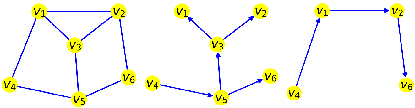
Figure 1: Here are two examples of directed subgraphs, $\hat{D}$ in the middle and $\bar{D}$ on the right, of a graph $G$ on the left. The directed subgraphs $\hat{D}$ and $\bar{D}$ can be considered as strategies to broadcast the messages in the graph $G$.

Example III.0.1.

Figure 1 illustrates two directed subgraphs $\hat{D}$ and $\bar{D}$ of a graph $G$. The following matrices $X$ and $Y$ are the matrix representations of $\hat{D}$ and $\bar{D}$ respectively.

$$X=\begin{pmatrix}0&0&0&0&0&0\\ 0&0&0&0&0&0\\ 1&1&0&0&0&0\\ 1&1&1&0&1&1\\ 1&1&1&0&0&1\\ 0&0&0&0&0&0\end{pmatrix}\hfil Y=\begin{pmatrix}0&1&0&0&0&1\\ 0&0&0&0&0&1\\ 0&0&0&0&0&0\\ 1&1&0&0&0&1\\ 0&0&0&0&0&0\\ 0&0&0&0&0&0\end{pmatrix}$$

The directed subgraphs $\hat{D}$ and $\bar{D}$ can be considered as strategies to broadcast the messages in the graph $G$, and their matrix representations make these strategies implementable.

The definition of matrix representation gives a map from the set of all directed subgraphs of $G$, denoted by $\mathsf{DirSub}(G)$, to the set of $|V|\times|V|$ matrices, denoted by $\mathsf{Mat}_{|V|}(\mathbb{R})$. Taking $\mathsf{MatRep}(G)$ as the image of this map, we get the following surjective function.

$$\mathsf{Rep}:\mathsf{DirSub}(G)\rightarrow\mathsf{MatRep}(G)$$

The following theorem shows the uniqueness of matrix representations for directed subgraphs. So, every directed subgraph can be determined completely by its representation.

Theorem III.1.

$\mathsf{Rep}$ is an isomorphism.

III-B Defining Covers for Graphs: An Algebraic Platform

While it is possible to cover a graph $G$ with a collection of elements from $\mathsf{DirSub}(G)$, and their matrix interpretation is accessible through $\mathsf{Rep}$, it is important to note that $\mathsf{DirSub}(G)$ is relatively small and lacks interaction among its elements. For example, the combination of $\hat{D}$ and $\bar{D}$, directed subgraphs presented in Figure 1, does not constitute a directed subgraph due to the presence of multiple paths between nodes. Consequently, its matrix interpretation does not exist, hindering its implementation in a message-passing process. This limitation poses challenges in designing diverse and meaningful strategies for message passing. To overcome this limitation and generate a more comprehensive set of elements, a method for combining them is required. Aiming for a broader space involves identifying an algebraic operation on $\mathsf{DirSub}(G)$. Pursuing a monoidal structure for $\mathsf{DirSub}(G)$, a common approach when transforming a set into an algebraic structure, seems appropriate. The operation $\bigoplus$ defined as follows can be a candidate. For $C,D\in\mathsf{DirSub}(G)$, the directed multigraph $C\bigoplus D$ is formed by taking the union of the sets of nodes and the disjoint union of the sets of directed edges. Thus, we have the commutative monoid $(\mathsf{Mult}(G),\bigoplus)$, where $\mathsf{Mult}(G)$ is defined as follows:

$\mathsf{Mult}(G)=\{\bigoplus_{i=1}^{k}D_{i}:\textit{for some }k\textit{ and }D_{1},\ldots,D_{k}\in\mathsf{DirSub}(G)\}$

In a multigraph, where multiple edges can exist between two nodes, the edges traversed by a path become crucial for specifying that path. This is why we highlight the edges between nodes in Definition III.0.1. Consequently, this definition of a path is applicable to multigraphs as well. The combination of two directed subgraphs using the $\bigoplus$ operator results in an element that lacks substantial inheritance from its generators. The paths within the two generators play a limited role in determining the paths of the resulting element. Instead, the generated element has all paths formed by concatenating directed edges from its generators. Consequently, the $\bigoplus$ operation exhibits limited capability to generate innovative strategies for message passing. To address this, there is a need for an operation that demonstrates heightened sensitivity towards the paths within directed subgraphs. The subsequent theorem introduces a monoidal operation that extends beyond $\bigoplus$ and emphasizes the pivotal role of paths in strategy development. In this theorem and also throughout this paper, we are influenced by category theory, choosing to use the term composition instead of concatenation when referring to the amalgamation of two paths.

Theorem III.2.

Let

$$\mathsf{SMult}(G)=\{(M,S):M\in\mathsf{Mult}(G),S\subseteq\mathsf{Paths}(M)\}$$

and the operation $\bullet$ be defined on $\mathsf{SMult}(G)$ as $(M,S)\bullet(N,T)=(M\bigoplus N,S\star T)$, where $S\star T$ is the union of the sets $S$, $T$, and the collection of paths constructed by the composition of paths in $S$ followed by paths in $T$. Then $(\mathsf{SMult}(G),\bullet)$ is a non-commutative monoid.

Note that in the above theorem, since the directed edges of $M\bigoplus N$ are obtained from the disjoint union of the directed edges of $M$ and $N$, the sets $S$ and $T$ are disjoint sets of paths as the subsets of $\mathsf{Paths}(M\bigoplus N)$. The operation $\bullet$ that acts as composition in categories allows the creation of the elements with allowed paths as desired. Non-commutativity of this operation comes from the composition of paths in the operation $\star$. If $(M,S),(N,T)\in\mathsf{SMult}(G)$ do not have composable paths, then $\star$ is reduced to the union of $S$ and $T$, hence $(M,S)\bullet(N,T)=(N,T)\bullet(M,S)$. In the following example, we show how the non-commutativity of $\bullet$ yields different elements by presenting a simple example.

Example III.2.1.

For directed edges $d:u\rightarrow v$ and $e:v\rightarrow w$, the elements $d\bullet e$ and $e\bullet d$ are distinct. While both share the same directed edges in $d\bigoplus e$ as illustrated in , they differ in terms of allowed paths. $d\bullet e$ includes a path from $u$ to $w$, whereas $e\bullet d$ lacks such a path. This highlights that the order of composition matters, resulting in different sets of allowed paths.

Considering $(M,S)$ in $\mathsf{SMult}(G)$ as a strategy for message passing, a multigraph is determined by $M$, and $S$ provides information about the allowed paths in $M$ for transferring messages. This monoid appears to be the appropriate place to define a cover as a collection of message-passing strategies. However, not all elements can be transformed into matrix form through an extension of $\mathsf{Rep}$, and as a result, implementing strategies becomes challenging. To address this, we focus on selecting elements that can be transformed. By leveraging the fact that the set $\mathsf{DirSub}(G)$ can be embedded in $\mathsf{SMult}(G)$ by associating a directed subgraph $D$ with $(D,\mathsf{Paths}(D))$, we construct a suitable monoid for our objectives:

Definition III.2.1.

For a graph $G=(V,E)$, we define the monoid of the directed subgraphs of $G$ to be the submonoid of $\mathsf{SMult}(G)$ generated by $\mathsf{DirSub}(G)$ and denote it by $\mathsf{Mod}(G)$.

Hence, for an object $(M,S)$ in $\mathsf{Mod}(G)$, there are some directed subgraphs $D_{1},\dots,D_{k}$ of $G$ such that $(M,S)=D_{1}\bullet\dots\bullet D_{k}$ and so $M=\bigoplus_{i=1}^{k}D_{i}$ and $S=\mathsf{Paths}(D_{1})\star\dots\star\mathsf{Paths}(D_{k})$. In the upcoming subsection, we aim to demonstrate that all elements belonging to the monoid $\mathsf{Mod}(G)$ can be transformed into matrix forms through an extension of $\mathsf{Rep}$. This characteristic makes the monoid a valuable tool in achieving our goal of assigning meaning to the concept of covers for graphs. We define a cover for a graph as follows:

Definition III.2.2.

A cover for a graph $G$ is a collection of finitely many elements of $\mathsf{Mod}(G)$.

A cover, as defined, specifies a view of the graph and establishes some rules for its internal interactions. Within each element of $\mathsf{Mod}(G)$ lies a set of allowed paths that describe a localized strategy in transfers, and a cover as a collection of them can be seen as a collection of traffic rules. Benefiting from $\bullet$, the elements of a cover are capable of being integrated as well as interacting with each other. We have not mentioned in the definition that a cover must coat all nodes or edges. This gives the flexibility to select a cover suitable for a desired task.

With infinitely many elements and the noncommutative monoidal operation, $\mathsf{Mod}(G)$ greatly increases our ability to convert different perspectives and message-passing strategies to the covers. Also, the following theorem confirms the simplicity of making arbitrary elements and shows that the set of all directed edges generates $\mathsf{Mod}(G)$, so these elements together with the monoidal operation $\bullet$ are enough to construct suitable elements of the monoid $\mathsf{Mod}(G)$ to use in a cover. The cover presented in subsequent section exemplifies applying this theorem.

Theorem III.3.

Directed edges generate $\mathsf{Mod}(G)$.

III-C From Covers to Matrices: An Algebraic Perspective

In this section, our objective is to extend the morphism $\mathsf{Rep}$ to a monoidal homomorphism, encompassing $\mathsf{Mod}(G)$ as its domain. This extension plays a pivotal role in the GGNN framework, transforming a cover into a collection of matrices. Since $\mathsf{Mod}(G)$ extends $\mathsf{DirSub}(G)$, we aim to move beyond $\mathsf{MatRep}(G)$ and enter a broader realm where matrix transformations corresponding to elements of $\mathsf{Mod}(G)$ reside. At first, we define the binary operation $\circ$ on $\mathsf{Mat}_{n}(\mathbb{R})$, the set of all $n\times n$ matrices, as follows:

$$A\circ B=A+B+AB$$

Theorem III.4.

$(\mathsf{Mat}_{n}(\mathbb{R}),\circ)$ is a monoid.

Now we are ready to extend $\mathsf{MatRep}(G)$ to a monoid:

Definition III.4.1.

The monoid of matrix representations of a given graph $G=(V,E)$ is defined to be the submonoid of $(\mathsf{Mat}_{|V|}(\mathbb{R}),\circ)$ generated by $\mathsf{MatRep}(G)$, denoted by $(\mathsf{Mom}(G),\circ)$.

To define a monoidal homomorphism between the monoids $(\mathsf{Mod}(G),\bullet)$ and $(\mathsf{Mom}(G),\circ)$ in such a way that it is an extension of the morphism $\mathsf{Rep}$, we need the following theorem which gives a good explanation of the monoidal operation $\circ$.

Theorem III.5.

For $A_{1},A_{2},\cdots,A_{k}\in\mathsf{Mat}_{n}(\mathbb{R})$ with $k\in\mathbb{N}$ we have:

$$\begin{split}A_{1}\circ A_{2}\circ\cdots\circ A_{k}&=\sum_{i=1}^{k}A_{i}\\ &+\sum_{\sigma\in O(k,2)}A_{\sigma_{1}}A_{\sigma_{2}}+\cdots\\ &+\sum_{\sigma\in O(k,j)}A_{\sigma_{1}}\cdots A_{\sigma_{j}}+\cdots\\ &+A_{1}A_{2}\cdots A_{k}\end{split}$$

where $O(k,i)$ is the set of all strictly monotonically increasing sequences of $i$ numbers of $\{1,\cdots,k\}$

Now, we present the extension of $\mathsf{Rep}$ as a monoidal homomorphism, mapping elements of $\mathsf{Mod}(G)$ to elements of $\mathsf{Mom}(G)$ while preserving the monoidal operations.

Theorem III.6.

The mapping $\mathsf{Tr}:\mathsf{Mod}(G)\longrightarrow\mathsf{Mom}(G)$

$$(M,S)=D_{1}\bullet D_{2}\bullet\cdots\bullet D_{k}\longmapsto A=A_{1}\circ A_{2}\circ\cdots\circ A_{k}$$

is a surjective monoidal homomorphism, where $D_{i}\in\mathsf{DirSub}(G)$ and $A_{i}=\mathsf{Rep}(D_{i})$.

We refer to $\mathsf{Tr}(M,S)$ as the matrix transformation of $(M,S)$. In the proof of Theorem III.6, it becomes evident that $\mathsf{Tr}$ functions as a path counter, assigning the number of paths in $S$ between two nodes $v_{i}$ and $v_{j}$ to the entry $ij$ of the matrix $\mathsf{Tr}(M,S)$. This monoidal surjection interprets covers as collections of matrices, establishing a relationship similar to that between the adjacency matrix and neighborhoods. While our attempts to establish $\mathsf{Tr}$ as an isomorphism have not succeeded, its nature as an extension of an isomorphism, coupled with its ability to characterize a graph up to isomorphism (as we will show in the next subsection), reinforces the validity of the matrix transformations derived from it for covers. Given the surjective nature of $\mathsf{Tr}$, we have:

Corollary III.6.1.

Matrix representations of directed edges generate $\mathsf{Mom}(G)$.

Example III.6.1.

In Example III.0.1, we considered two directed subgraphs, $\hat{D}$ and $\bar{D}$, of a graph $G$ as illustrated in Figure 1, and provided their respective matrix representations, denoted as $X$ and $Y$. We highlighted that these subgraphs can be viewed as strategies for broadcasting messages within the graph. Through the operation $\bullet$, we can combine them to form new strategies, $\hat{D}\bullet\bar{D}$ and $\bar{D}\bullet\hat{D}$. Utilizing the matrix transformations obtained via $\mathsf{Tr}$, we can implement these combined strategies for the message-passing process.

$\mathsf{Tr}(\hat{D}\bullet\bar{D})=\mathsf{Tr}(\hat{D})\circ\mathsf{Tr}(\bar{D})=X\circ Y=\begin{pmatrix}0&1&0&0&0&1\\ 0&0&0&0&0&1\\ 1&2&0&0&0&2\\ 2&3&1&0&1&4\\ 1&2&1&0&0&3\\ 0&0&0&0&0&0\end{pmatrix}$

$\hfil\mathsf{Tr}(\bar{D}\bullet\hat{D})=\mathsf{Tr}(\bar{D})\circ\mathsf{Tr}(\hat{D})=Y\circ X=\begin{pmatrix}0&1&0&0&0&1\\ 0&0&0&0&0&1\\ 1&1&0&0&0&0\\ 2&2&1&0&1&2\\ 1&1&1&0&0&1\\ 0&0&0&0&0&0\end{pmatrix}$

IV Grothendieck Graph Neural Networks Framework

IV-A Algebraic Foundations of Graphs

So far, for an arbitrary graph, two monoids and a monoidal homomorphism between them have been presented. The question that arises now is how much these monoidal structures can describe a graph. To answer this question, some preliminaries are needed. We define a special type of linear isomorphism between vector space of matrices. A matrix $A\in\mathsf{Mat}_{n}(\mathbb{R})$ is actually a linear transformation from $\mathbb{R}^{n}$ to itself. Reordering the standard basis of $\mathbb{R}^{n}$ changes the matrix representation of the linear transformation in such a way that it will be obtained by reordering rows and columns of matrix $A$. These actions change the indices of entries of $A$; so a change in the order of the standard basis of $\mathbb{R}^{n}$ gives a linear isomorphism from $\mathsf{Mat}_{n}(\mathbb{R})$ to itself. We call this kind of linear isomorphism a Change-of-Order mapping. We give a simple example:

Example IV.0.1.

Considering a Change-of-Order mapping $f:\mathsf{Mat}_{3}(\mathbb{R})\rightarrow\mathsf{Mat}_{3}(\mathbb{R})$, obtained by reordering the standard basis $\{e_{1},e_{2},e_{3}\}$ to the basis $\{e_{3},e_{2},e_{1}\}$. For a given matrix $A$, we get the matrix $f(A)$ as follows:

$$A\longmapsto f(A)$$

$$\bordermatrix{&e_{1}&e_{2}&e_{3}\cr e_{1}&a_{11}&a_{12}&a_{13}\cr e_{2}&a_{21}&a_{22}&a_{23}\cr e_{3}&a_{31}&a_{32}&a_{33}}\lx@xy@svg{\hbox{\raise 0.0pt\hbox{\kern 3.0pt\hbox{\ignorespaces\ignorespaces\ignorespaces\hbox{\vtop{\kern 0.0pt\offinterlineskip\halign{\entry@#!@&&\entry@@#!@\cr&\crcr}}}\ignorespaces{\hbox{\kern-3.0pt\raise 0.0pt\hbox{\hbox{\kern 0.0pt\raise 0.0pt\hbox{\hbox{\kern 3.0pt\raise 0.0pt\hbox{$\textstyle{\ignorespaces\ignorespaces\ignorespaces\ignorespaces}$}}}}}}}\ignorespaces\ignorespaces\ignorespaces\ignorespaces{\hbox{\kern 3.0pt\raise 0.0pt\hbox{\hbox{\kern 0.0pt\raise 0.0pt\hbox{\lx@xy@stopper}}}}}{\hbox{\lx@xy@droprule}}\ignorespaces\ignorespaces\ignorespaces{\hbox{\kern 0.1781pt\raise 6.1111pt\hbox{{}\hbox{\kern 0.0pt\raise 0.0pt\hbox{\hbox{\kern 3.0pt\hbox{\hbox{\kern 0.0pt\raise-1.75pt\hbox{$\scriptstyle{f:e_{1}\leftrightarrow e_{3}}$}}}\kern 3.0pt}}}}}}\ignorespaces{\hbox{\kern 27.0pt\raise 0.0pt\hbox{\hbox{\kern 0.0pt\raise 0.0pt\hbox{\lx@xy@tip{1}\lx@xy@tip{-1}}}}}}{\hbox{\lx@xy@droprule}}{\hbox{\lx@xy@droprule}}{\hbox{\kern 27.0pt\raise 0.0pt\hbox{\hbox{\kern 0.0pt\raise 0.0pt\hbox{\hbox{\kern 3.0pt\raise 0.0pt\hbox{$\textstyle{}$}}}}}}}\ignorespaces}}}}\ignorespaces\bordermatrix{&e_{3}&e_{2}&e_{1}\cr e_{3}&a_{33}&a_{32}&a_{31}\cr e_{2}&a_{23}&a_{22}&a_{21}\cr e_{1}&a_{13}&a_{12}&a_{11}} \scriptstyle{f:e_{1}\leftrightarrow e_{3}}$$

The Change-of-Order mappings are compatible with the monoidal structure of $\mathsf{Mat}_{n}(\mathbb{R})$ as shown in the following Theorem:

Theorem IV.1.

Suppose $f:\mathsf{Mat}_{n}(\mathbb{R})\rightarrow\mathsf{Mat}_{n}(\mathbb{R})$ is a Change-of-Order mapping. Then $f$ preserves $\circ$, matrix multiplication and element-wise multiplication.

Now, we want to investigate the effect of two isomorphic graphs on their corresponding monoidal structures and vice versa. A graph isomorphism $f:G\rightarrow H$ is a change in the chosen order of the nodes. So it induces a Change-of-Order mapping $\mathsf{CO}(f):\mathsf{Mat}_{|V_{G}|}(\mathbb{R})\rightarrow\mathsf{Mat}_{|V_{H}|}(\mathbb{R})$. The following theorem shows that isomorphic graphs have isomorphic monoidal structures described in Theorem III.6.

Theorem IV.2.

Every graph isomorphism $f:G\rightarrow H$ induces monoidal isomorphisms $\mathsf{Mod}(f):\mathsf{Mod}(G)\longrightarrow\mathsf{Mod}(H)$ and $\mathsf{Mom}(f):\mathsf{Mom}(G)\rightarrow\mathsf{Mom}(H)$ such that the Diagram 1 is commutative, where $\iota$ represents the inclusions.

(1)

The converse of Theorem IV.2 can be stated as follows:

Theorem IV.3.

Suppose $G$ and $H$ are two graphs with $|V_{G}|=|V_{H}|=n$, and $f:\mathsf{Mat}_{n}(\mathbb{R})\rightarrow\mathsf{Mat}_{n}(\mathbb{R})$ is a Change-of-Order mapping. If the restriction of $f$ to $\mathsf{Mom}(G)$ yields an isomorphism to $\mathsf{Mom}(H)$, then $G$ and $H$ are isomorphic.

IV-B Definition of the GGNN Framework

Theorems IV.2 and IV.3 lay the foundation for our framework. These theorems establish that graphs $G$ and $H$ are isomorphic if and only if the vertical homomorphisms in Diagram 1 are isomorphisms. This crucially implies that altering the node order in a graph induces isomorphic changes in both a cover and its matrix interpretation. Thus, the horizontal homomorphisms in Diagram 1 serve as a complete determination of graphs, providing algebraic descriptions for them. Leveraging this diagram, we define the GGNN framework as follows:

Definition IV.3.1.

The Grothendieck Graph Neural Networks framework for a graph $G$ is defined to be the algebraic description:

(2)

The GGNN framework introduces various actions for creating, translating, and enriching a cover. $\mathsf{Mod}(G)$ offers multiple choices of covers, serving as alternatives for cover of neighborhoods. The transformation $\mathsf{Tr}$ converts these covers into collections of matrices, and, with the mapping $\iota$, these collections are transported to a larger space, providing an opportunity to enrich them using elements of $\mathsf{Mat}_{|V_{G}|}(\mathbb{R})$ and the allowed operation presented in Theorem IV.1. The process of designing a GNN model within this framework is outlined as follows:

• For a given graph $G$, the process involves selecting a collection $\mathcal{C}_{G}$ of elements from $\mathsf{Mod}(G)$ to serve as a cover for $G$. These elements can be generated using $\mathsf{DirSub}(G)$ and the binary operation $\bullet$. Notably, Theorem III.3 ensures the ability to create any suitable and desired elements by leveraging directed edges and the operator $\bullet$.

• Next, the chosen cover is transformed into a collection of matrices within $\mathsf{Mom}(G)$. During this transformation, the operation $\circ$ and other elements of $\mathsf{Mom}(G)$ can be employed to convert the original collection into a new one. The resulting output at this stage is denoted by $\mathcal{A}_{G}$.

• By utilizing $\iota$, the collection obtained in the second stage transitions into a larger and more equipped space, a suitable environment for enrichment. This stage leverages all the operations outlined in Theorem IV.1 to complete the model’s design. Following the processing of $\mathcal{A}_{G}$ in this stage, we obtain a new collection of matrices denoted by $\mathcal{M}_{G}$, representing the model’s output.

Hence, a model is a mapping that associates a collection of matrices $\mathcal{M}_{G}$ with a given graph $G$. $\mathcal{M}_{G}$ plays a role akin to the adjacency matrix and provides an interpretation of the chosen cover for use in various forms of message passing. While the second and third stages can be merged, we prefer to emphasize the significance of $\mathsf{Tr}$ in this process.

This construction of a model is appropriate for tasks such as node classification. For graph isomorphism and classification tasks, we need an invariant construction. Based on the Theorem IV.2, a graph isomorphism $f:G\rightarrow H$ transform the triple $(\mathcal{C}_{G},\mathcal{A}_{G},\mathcal{M}_{G})$ to a triple $(\mathcal{C}^{\prime}_{H},\mathcal{A}^{\prime}_{H},\mathcal{M}^{\prime}_{H})$ for graph $H$ and this may be different from $(\mathcal{C}_{H},\mathcal{A}_{H},\mathcal{M}_{H})$. So a model constructed in the GGNN framework is invariant if for every graph isomorphism $f:G\rightarrow H$, the maps $\mathsf{Mod}(f)$, $\mathsf{Mom}(f)$ and $\mathsf{CO}(f)$ induce one-to-one correspondences between $\mathcal{C}_{G}$ and $\mathcal{C}_{H}$, $\mathcal{A}_{G}$ and $\mathcal{A}_{H}$, and $\mathcal{M}_{G}$ and $\mathcal{M}_{H}$, respectively. The model presented in the next section is an example of an invariant model.

IV-C The Cover of Neighborhoods in the GGNN Framework

The role of neighborhoods in MPNN is like a sink such that messages move to the center of the sink. For a node $v_{k}$ with neighborhood $N_{k}$ containing $v_{k_{1}},v_{k_{2}},\cdots,v_{k_{m}}$, we depict this sink in Figure 2 by denoting directed edge from $v_{k_{i}}$ to $v_{k}$ by $e_{i}:v_{k_{i}}\rightarrow v_{k}$.

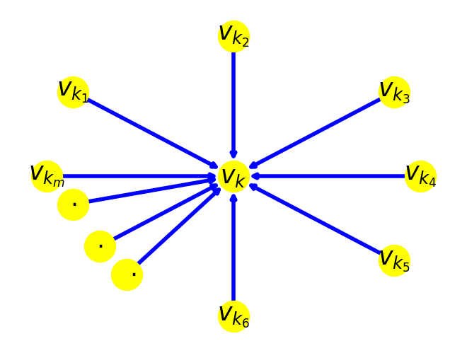
Figure 2: Visualizing a neighborhood by representing it as a directed subgraph

This sink can be considered as a directed subgraph. As an element of $\mathsf{Mod}(G)$, it can be represented as follows:

$$S_{k}=e_{1}\bullet e_{2}\bullet\cdots\bullet e_{m}$$

Since the directed edges $e_{i}$ and $e_{j}$ appearing in $S_{k}$ are not composable, we observe $e_{i}\bullet e_{j}=e_{j}\bullet e_{i}$, rendering the order in $S_{k}$ unimportant. The cover obtained by $S_{k}$s is exactly the cover of the neighborhoods. Let $T_{k}=\mathsf{Tr}(S_{k})$ and $A_{i}=\mathsf{Tr}(e_{i})$. Thus $A_{i}$ has $1$ in the entry $k_{i}k$ and $0$ for all other entries. The matrix transformation of $e_{i}\bullet e_{j}$ has just two non-zero entries and $\mathsf{Tr}(e_{i}\bullet e_{j})=A_{i}+A_{j}+A_{i}A_{j}$. Then $A_{i}A_{j}=0$ for $1\leq i\leq m$ and $1\leq j\leq m$. Theorem III.5 implies

$$\begin{split}T_{k}=\mathsf{Tr}(S_{k})&=A_{1}\circ A_{2}\circ\cdots\circ A_{m}\\ &=A_{1}+A_{2}+\cdots+A_{m}\end{split}$$

As a result, the column $k$ of $T_{k}$ aligns with the column $k$ of the adjacency matrix of graph $G$, while the remaining columns are filled with zeros. Transforming the cover $\{S_{k}\}$ yields a collection of $|V|$ matrices, each containing a single column from the adjacency matrix. In the GGNN framework, summation is an allowed operation, enabling the construction of the adjacency matrix by performing the summation on this matrix collection. Hence, neighborhoods can function as a cover within the framework of GGNN, with the adjacency matrix serving as an interpretation of this cover.

The cover of neighborhoods, as a subset of $\mathsf{Mod}(G)$, generates a submonoid. To formalize this, let $\mathsf{Neigh}(G)\subseteq\mathsf{Mod}(G)$ and $\mathsf{Adj}(G)\subseteq\mathsf{Mom}(G)$ denote the submonoids generated by the cover of neighborhoods and its matrix transformation, respectively. The following theorems illustrate how these submonoids provide an algebraic characterization of a graph. It is straightforward to verify that for a graph isomorphism $f:G\to H$, the mappings $\mathsf{Mod}(f)$ and $\mathsf{Mom}(f)$ send elements of $\mathsf{Neigh}(G)$ and $\mathsf{Adj}(G)$ to elements of $\mathsf{Neigh}(H)$ and $\mathsf{Adj}(H)$, respectively. Thus, as a consequence of Theorem IV.2, we have:

Theorem IV.4.

Every graph isomorphism $f:G\rightarrow H$ induces monoidal isomorphisms $\mathsf{Neigh}(f):\mathsf{Neigh}(G)\longrightarrow\mathsf{Neigh}(H)$ and $\mathsf{Adj}(f):\mathsf{Adj}(G)\rightarrow\mathsf{Adj}(H)$ such that the following diagram is commutative, where $\iota$ represents the inclusions.

(3)

The converse of this theorem can be stated as follows:

Theorem IV.5.

Suppose $G$ and $H$ are two graphs with $|V_{G}|=|V_{H}|=n$, and $f:\mathsf{Mat}_{n}(\mathbb{R})\rightarrow\mathsf{Mat}_{n}(\mathbb{R})$ is a Change-of-Order mapping. If the restriction of $f$ to $\mathsf{Adj}(G)$ yields an isomorphism to $\mathsf{Adj}(H)$, then $G$ and $H$ are isomorphic.

Consequently, the horizontal homomorphisms in Diagram 3 can serve as an algebraic description of the graph. Thus, the cover of neighborhoods can be further enriched by incorporating additional elements from $\mathsf{Neigh}(G)$.

IV-D GGNN Framework vs. Higher-Order GNNs: A Comparison

We aim to highlight several advantages of the GGNN framework compared to higher-order GNNs, such as MPSN [5], CWN [6], GSN [11], and TLGNN [10].

The first key advantage of the GGNN framework is that it is not a model but a versatile framework. It provides the ability to define covers through precise mathematical definitions, applicable to any arbitrary graph, much like how neighborhoods are defined. While higher-order GNNs propose specific alternatives for message passing, GGNN allows for the construction of infinitely many alternatives (covers) for the concept of neighborhoods. These alternatives, as shown in our work, are natural extensions of the neighborhood concept and can be exploited to create diverse GNN architectures.

The second advantage is that the GGNN framework enables the design of topology-aware GNNs. As established in Theorems IV.2 and IV.3, GGNN provides a unique, up-to-isomorphism algebraic description for graphs. Each monoidal element of $\mathsf{Mod}(G)$ encodes specific topological characteristics of the graph $G$. By selecting appropriate covers, one can effectively capture desired topological properties of the graph. Moreover, the tools provided within the GGNN framework facilitate the creation of GNNs that incorporate ideas from other GNN paradigms.

For example, we can construct a GNN within the GGNN framework that mirrors the functionality of $K$-hop message passing GNNs as presented in [14]:

Example IV.5.1.

Using the cover of neighborhoods $\{S_{v}:v\in G\}$, we construct a new cover for the graph $G$ comparable to $K$-hop message passing GNNs. For each node $v_{k}$, we associate a collection of monoidal elements as follows:

$$2\text{-}\mathsf{hop}(v_{k})=\{S_{v_{k_{i}}}\bullet e_{i}:v_{k_{i}}\in N(v_{k})\text{ and }e_{i}:v_{k_{i}}\rightarrow v_{k}\}$$

We define the cover $2\text{-}\mathsf{hop}(G)$ as the union of all $2\text{-}\mathsf{hop}(v_{k})$. By applying $\mathsf{Tr}$ to this cover, we obtain a collection of matrices, which can then be unified by summing all the matrices in the collection.

While we do not delve into the details of this example here, in the next section, we introduce a novel cover inspired by the concept of sieves in category theory. This cover leverages a precise definition of certain elements in $\mathsf{Mod}(G)$ as an extension of the traditional neighborhood definition.

V Sieve Neural Network, A model Based on GGNN framework

Based on the concept of sieves in category theory, we will introduce a GNN model, called Sieve Neural Networks ($\mathsf{SNN}$), which will be constructed in the GGNN framework. In this model, each node spreads its roots in the graph like a growing seed and tries to feed itself through these roots. We mean this story by creating appropriate elements of $\mathsf{Mod}(G)$ for a graph $G$ and considering their collection as a cover for the graph. The connections resulting from this cover provide various ways for message passing between nodes that lead to a knowledge of the graph topology. In the following, we explain the process of creating the desired cover and introduce the model based on them.

V-A Cover of Sieves for Graphs

Generating the desired elements of $\mathsf{Mod}(G)$: Start with a graph $G=(V,E)$. For each node, we create the following sets of directed edges:

Let $v\in V$ and $N(v)$ be its neighborhood.

• $N_{0}(v)=\{v\}$

  $M_{0}=\emptyset$
  

• $N_{1}(v)=N(v)$

  $M_{1}(v)=\{w\rightarrow u:wu\in E,w\in N_{1}(v),u\in N_{0}(v)\}$
  

• $N_{2}(v)=\bigcup_{u\in N_{1}(v)}N(u)-(N_{1}(v)\cup N_{0}(v))$,

  $M_{2}(v)=\{w\rightarrow u:wu\in E,w\in N_{2}(v),u\in N_{1}(v)\}$
  

  $\vdots$
  

• $N_{k}(v)=\bigcup_{u\in N_{k-1}(v)}N(u)-\bigcup_{i=0}^{k-1}N_{i}(v)$,

  $M_{k}(v)=\{w\rightarrow u:wu\in E,w\in N_{k}(v),u\in N_{k-1}(v)\}$
  

  $\vdots$

The directed edges in $M_{i}(v)$ are not composable. Therefore, disregarding the order and non-commutativity of $\bullet$, we define

$$D_{i}(v):={{\bullet}}e_{{}_{e\in M_{i}(v)}}$$

and utilizing them to generate the elements

$$\mathsf{Sieve}(v,k):=D_{k}(v)\bullet D_{k-1}(v)\bullet\cdots\bullet D_{1}(v)\bullet D_{0}(v)$$

of $\mathsf{Mod}(G)$ in which $D_{0}(v)$ is the identity of $\mathsf{Mod}(G)$, see Figure 3. Obviously there is some $k_{0}$ such that $M_{k}\neq\emptyset$ and $\emptyset=M_{k_{0}+1}=M_{k_{0}+2}=\cdots$. Then

$$\mathsf{Sieve}(v,k_{0})=\mathsf{Sieve}(v,k_{0}+1)=\mathsf{Sieve}(v,k_{0}+2)=\cdots$$

We denote the element $\mathsf{Sieve}(v,k_{0})$ by $\mathsf{Sieve}(v,-1)$.

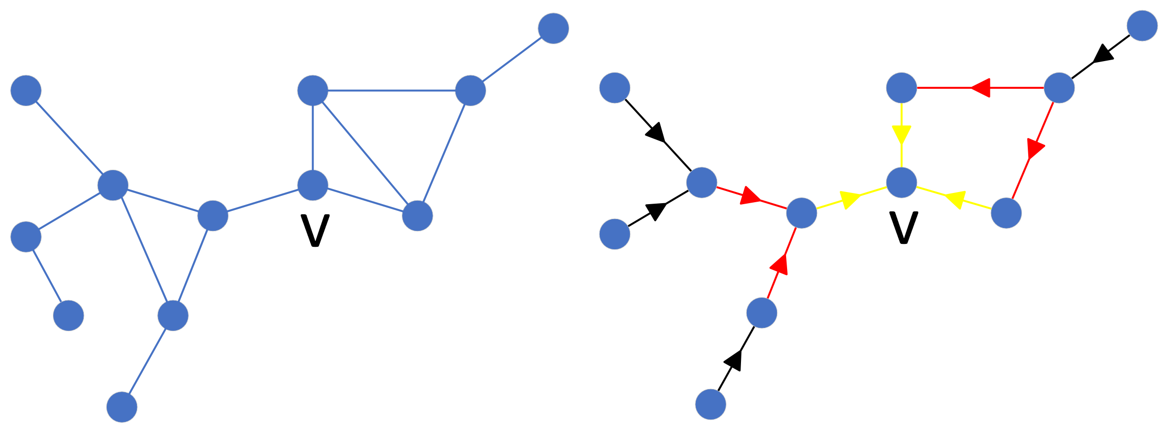
Figure 3: Left: A graph $G$. Right: $\mathsf{Sieve}(v,3)=D_{3}(v)\bullet D_{2}(v)\bullet D_{1}(v)$. Directed edges in yellow, red and black specify $D_{1}(v)$, $D_{2}(v)$ and $D_{3}(v)$ recpectively

To construct the opposite of $\mathsf{Sieve}(v,k)$, we define $M^{op}_{i}(v)$ as the set containing the edges in $M_{i}(v)$ with the opposite directions. We then create

$$D_{i}^{op}(v):={{\bullet}}e_{{}_{e\in M_{i}^{op}(v)}}$$

This results in new elements of $\mathsf{Mod}(G)$, defined as follows:

$$\mathsf{CoSieve}(v,l):=D_{0}^{op}(v)\bullet D_{1}^{op}(v)\bullet\cdots\bullet D_{l-1}^{op}(v)\bullet D_{l}^{op}(v)$$

.

The Cover of Sieves: So far, for a graph $G$, the following elements of $\mathsf{Mod}(G)$ have been selected for every node $v$.

$$\mathsf{Sieve}(v,0),\mathsf{Sieve}(v,1),\cdots,\mathsf{Sieve}(v,-1)$$

$$\mathsf{CoSieve}(v,0),\mathsf{CoSieve}(v,1),\cdots,\mathsf{CoSieve}(v,-1)$$

Our desired cover for a graph $G$ is the collection containing all these elements for all nodes in $G$ and we call it the cover of sieves.

Matrix Interpretation of The Cover of Sieves: The mapping $\mathsf{Tr}$ gives the matrix interpretation of the cover of sieves, transforming it into a collection of elements of $\mathsf{Mom}(G)$, denoted as follows:

$\mathsf{Image}(v,k):=\mathsf{Tr}(\mathsf{Sieve}(v,k))$

$\mathsf{CoImage}(v,l):=\mathsf{Tr}(\mathsf{CoSieve}(v,l))$

Since $\mathsf{Tr}$ is a monoidal homomorphism, $\mathsf{Image}(v,k)$ can be expressed as follows, providing insight into its computational procedure:

$$\small\begin{split}\mathsf{Image}(v,k)&=\mathsf{Tr}(\mathsf{Sieve}(v,k))\\ &=\mathsf{Tr}(D_{k}(v)\bullet D_{k-1}(v)\bullet\cdots\bullet D_{0}(v))\\ &=\mathsf{Tr}(D_{k}(v))\circ\mathsf{Tr}(D_{k-1}(v))\circ\cdots\circ\mathsf{Tr}(D_{0}(v))\end{split}$$ (4)

Therefore, to calculate $\mathsf{Image}(v,k)$, it is necessary to transform $D_{i}(v)$ into matrix form. As we mentioned, directed edges in $M_{i}(v)$ are not composable. Then $\mathsf{Tr}(e)\mathsf{Tr}(c)=\mathsf{Tr}(c)\mathsf{Tr}(e)=0$ for $e,c\in M_{i}(v)$. Theorem III.5 implies:

$$\mathsf{Tr}(D_{i}(v))=\mathsf{Tr}({{\bullet}}e_{{}_{e\in M_{i}(v)}})={{\circ}}\mathsf{Tr}(e)_{{}_{e\in M_{i}(v)}}=\sum_{e\in M_{i}(v)}\mathsf{Tr}(e)$$

So obtaining $\mathsf{Tr}(D_{i}(v))$ is achievable from the adjacency matrix of $G$ based on the definition of $M_{i}$. It is easy to verify that $\mathsf{CoImage}(v,l)$ is the transpose of $\mathsf{Image}(v,l)$. Therefore, computing one of them is enough.

The following theorem demonstrates that the cover of sieves remains invariant under graph isomorphisms:

Theorem V.1.

Suppose $f:G\rightarrow H$ is a graph isomorphism. Then $\mathsf{Mod}(f)(\mathsf{Sieve}(v,k))=\mathsf{Sieve}(f(v),k)$ and $\mathsf{Mom}(f)(\mathsf{Image}(v,k))=\mathsf{Image}(f(v),k)$.

Furthermore, the submonoid generated by this cover fully determines the graph, as stated in the following two theorems. Let $\mathsf{Si}(G)\subseteq\mathsf{Mod}(G)$ and $\mathsf{Im}(G)\subseteq\mathsf{Mom}(G)$ denote the submonoids generated by the cover of sieves and its matrix transformation, respectively. As a direct consequence of Theorems V.1 and IV.2, we have:

Theorem V.2.

Every graph isomorphism $f:G\rightarrow H$ induces monoidal isomorphisms $\mathsf{Si}(f):\mathsf{Si}(G)\longrightarrow\mathsf{Si}(H)$ and $\mathsf{Im}(f):\mathsf{Im}(G)\rightarrow\mathsf{Im}(H)$ such that the Diagram 5 is commutative, where $\iota$ represents the inclusions.

(5)

The converse of the above theorem can be stated as follows:

Theorem V.3.

Suppose $G$ and $H$ are two graphs with $|V_{G}|=|V_{H}|=n$, and $f:\mathsf{Mat}_{n}(\mathbb{R})\rightarrow\mathsf{Mat}_{n}(\mathbb{R})$ is a Change-of-Order mapping. If the restriction of $f$ to $\mathsf{Im}(G)$ yields an isomorphism to $\mathsf{Im}(H)$, then $G$ and $H$ are isomorphic.

The next step is to develop an approach to transform the matrix interpretation of this cover into a unified matrix, which can serve as a replacement for the adjacency matrix. In the following, using the versions $\alpha$ and $\beta$ of $\mathsf{SNN}$, we introduce two approaches for integrating matrices derived from the matrix interpretation of the cover of sieves into a unified matrix.

V-B Design and Construction of the $\mathsf{SNN}$ Model

Based on the cover of sieves and its matrix interpretation, we present our model, $\mathsf{SNN}$, with varying levels of complexity as follows:

• $\mathsf{SNN}(\alpha,(l,k))$: In the $\alpha$ version of $\mathsf{SNN}$, $\mathsf{Sieve}(v,k)$ is considered as a receiver and $\mathsf{CoSieve}(v,l)$ as a sender for a node $v$. For nodes $v_{i}$ and $v_{j}$, the ways to transmit information from $v_{i}$ to $v_{j}$ are the allowed paths from $v_{i}$ to $v_{j}$ in

  $$\mathsf{CoSieve}(v_{i},l)\bullet\mathsf{Sieve}(v_{j},k)$$

  see Figure 4. The number of these paths is $ij$ entry of

  $$\mathsf{CoImage}(v_{i},l)\circ\mathsf{Image}(v_{j},k)$$

  By dividing this number by the product of the summation of entries in the $i$-th row of $\mathsf{CoImage}(v_{i},l)$ and the summation of entries in the $j$-th column of $\mathsf{Image}(v_{j},k)$, we obtain the ratio of established paths between $v_{i}$ and $v_{j}$ to the maximum expected paths. The matrix resulting from performing this process for all $i$s and $j$s is the output of $\mathsf{SNN}(\alpha,(l,k))$ for graph $G$. The division step is a way for preserving additional information from $\mathsf{CoSieve}(v_{i},l)\bullet\mathsf{Sieve}(v_{j},k)$ in the model’s output. Omitting this step results in denoting the model as $\mathsf{SNN}_{o}(\alpha,(l,k))$.

  

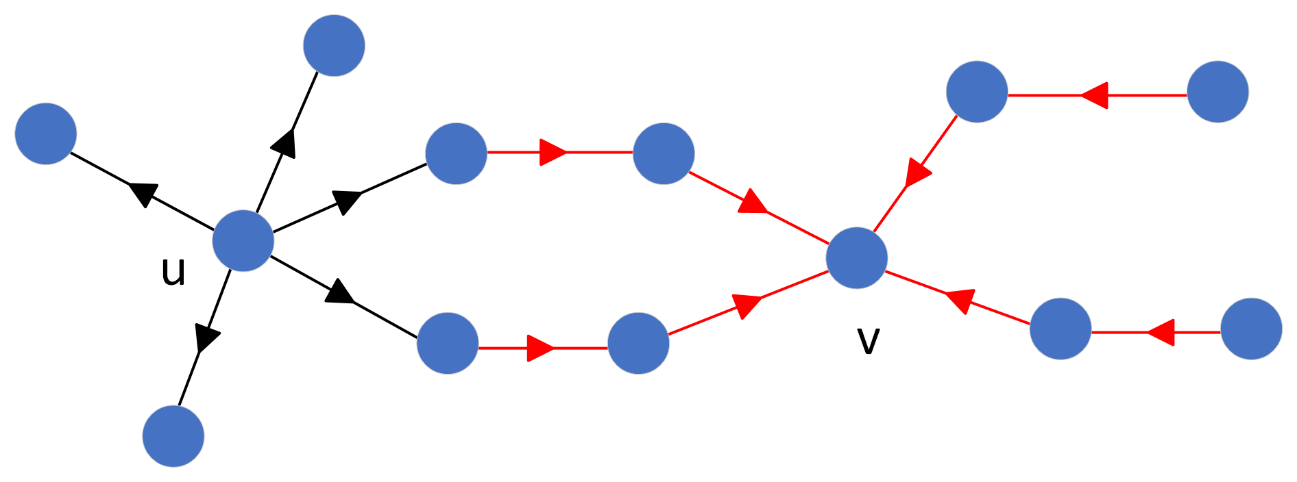
  Figure 4: $\mathsf{CoSieve}(u,1)\bullet\mathsf{Sieve}(v,2)$ as an element of $\mathsf{Mod}(G)$ determines the ways of establishing contact between $u$ and $v$ in $\mathsf{SNN}(\alpha,(1,2))$

• $\mathsf{SNN}(\beta,(l_{1},\cdots,l_{t}))$: In the $\beta$ version of $\mathsf{SNN}$, we leverage $\mathsf{Mat}_{n}(\mathbb{R})$ by mapping the collection of $\mathsf{Image}$s and $\mathsf{CoImage}$s into it. Here, additional operations become available, and we choose summation. For $l_{i}$, if $i$ is odd, we denote by $Su_{i}$ the summation (over nodes) of all matrices $\mathsf{CoImage}(v,l_{i})$ and if $i$ is even, $Su_{i}$ is the summation of all matrices $\mathsf{Image}(v,l_{i})$. Ultimately, the matrix $Su_{1}\circ\cdots\circ Su_{t}$ represents the output of $\mathsf{SNN}(\beta,(l_{1},\cdots,l_{t}))$ for graph $G$.

Utilizing the relationship $\mathsf{CoImage}(v_{i},l)=\mathsf{Image}(v_{i},l)^{tr}$, we derive $\mathsf{CoImage}(v_{i},l)\circ\mathsf{Image}(v_{j},k)=(\mathsf{CoImage}(v_{j},k)\circ\mathsf{Image}(v_{i},l))^{tr}$. Consequently, the output of $\mathsf{SNN}(\alpha,(l,k))$ is the transpose of the output of $\mathsf{SNN}(\alpha,(k,l))$. This symmetry implies that the output of $\mathsf{SNN}(\alpha,(l,l))$ is symmetric as well. Nonetheless, a comparative analysis allows us to conclude that $\mathsf{SNN}(\alpha,(l^{\prime},k^{\prime}))$ can capture more paths than $\mathsf{SNN}(\alpha,(l,k))$ if $l\leq l^{\prime}$ and $k\leq k^{\prime}$.

Version $\beta$ of $\mathsf{SNN}$ is designed to offer a more comprehensive representation of the cover of sieves. The collection $\{\mathsf{Sieve}(v,l_{i})\}$ (or $\{\mathsf{CoSieve}(v,l_{i})\}$) forms a subcover within the cover of sieves. The matrix $Su_{i}$ can be seen as an interpretation of this subcover, representing all allowed paths for the elements within it. By the element $Su_{1}\circ\cdots\circ Su_{t}$, we obtain a matrix that interprets a specific combination of these subcovers. This resulting matrix represents the paths formed by the composition of allowed paths from the mentioned subcovers, providing a distinct interpretation of the cover of sieves.

$\mathsf{SNN}$ transforms a dataset of graphs by replacing the adjacency matrix with its output. The resulting transformed dataset is well-suited as input for various GNN methods that rely on message passing. This transformation implies that any GNN can utilize the cover of sieves as an alternative to the traditional cover of neighborhoods. The following theorem establishes the invariance of $\mathsf{SNN}$, underscoring its effectiveness in graph isomorphism and classification tasks.

Theorem V.4.

$\mathsf{SNN}$ is invariant.

SNN in Practice: Most of the time, GNNs deal with featured graphs. In the case of $\mathsf{SNN}$, Equation 4 is the point to incorporate edge features. For a featured graph $G=(V,E,F)$ with edge features in $\mathbb{R}^{m}$, replacing $1$s with the corresponding edge features in $\mathsf{Tr}(D_{i}(v))$ yields a matrix where entries are sourced from $m$-dimensional vectors. Through the update operation $\circ$, employing element-wise summation and multiplication for $m$-dimensional vectors, $\mathsf{SNN}$ acquires the ability to deal with featured graphs. Additionally, by multiplying $\mathsf{Tr}(D_{i}(v))$s by a constant $\gamma\in(0,1]$, the model can be enhanced in a manner that is sensitive to the length of paths.

Comparing with MPNN: For a node $v$, its neighborhood can be described by the element $\mathsf{Sieve}(v,1)$. Consequently, $\mathsf{SNN}_{o}(\alpha,(0,1))$ and $\mathsf{SNN}_{o}(\alpha,(1,0))$ correspond to the adjacency matrix, signifying their utilization of neighborhoods for message passing. This is equivalent to MPNNs. Hence, $\mathsf{SNN}$ can be considered as a generalization of MPNNs. In the following example, two graphs are considered that MPNN can not distinguish, yet $\mathsf{SNN}$ can. This example illustrates how a shift in perspective, resulting from a change in cover, reveals the topological properties of graphs.

Example V.4.1.

The graphs in Figure 5 are not distinguishable by MPNN [2] because they are locally the same.

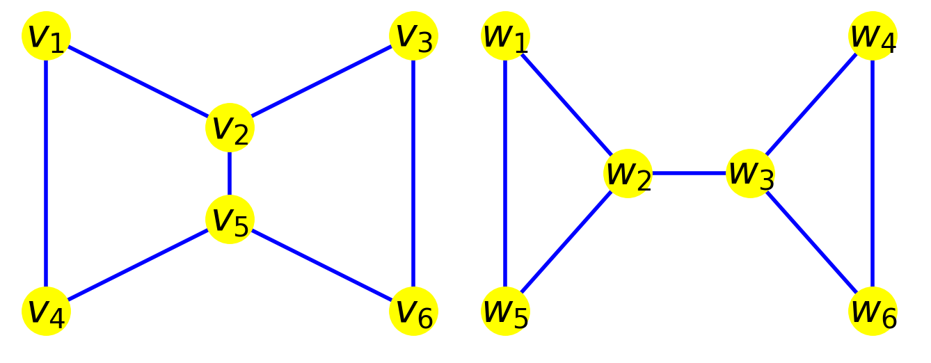
Figure 5: The graph $G$, the left one, and $H$, the right one, are not distinguishable by MPNN

Applying $\mathsf{SNN}_{o}(\alpha,(1,1))$, a level of version $\alpha$ of $\mathsf{SNN}$ that is slightly more potent than MPNN, we get the following symmetric matrices $X$ and $Y$ for $G$ and $H$ respectively as the outputs of the model for these graphs.

$X=\begin{pmatrix}2&2&1&2&2&0\\ 2&3&2&2&2&2\\ 1&2&2&0&2&2\\ 2&2&0&2&2&1\\ 2&2&2&2&3&2\\ 0&2&2&1&2&2\end{pmatrix},Y=\begin{pmatrix}2&3&1&0&3&0\\ 3&3&2&1&3&1\\ 1&2&3&3&1&3\\ 0&1&3&2&0&3\\ 3&3&1&0&2&0\\ 0&1&3&3&0&2\end{pmatrix}$

The entry $ij$ in these matrices corresponds to the count of paths between nodes $v_{i}$ and $v_{j}$ in $\mathsf{CoSieve}(v_{i},1)\bullet\mathsf{Sieve}(v_{j},1)$ and $w_{i}$ and $w_{j}$ in $\mathsf{CoSieve}(w_{i},1)\bullet\mathsf{Sieve}(w_{j},1)$. The disparity between these matrices highlights the differences between the graphs. This dissimilarity becomes more apparent when applying the set function $\mathsf{Var}$, while $\mathsf{Sum}$ and $\mathsf{Mean}$ yield identical values. When $\mathsf{SNN}_{o}(\alpha,(1,2))$, a more complex level of $\mathsf{SNN}$, is applied, we obtain the following nonsymmetric matrices, denoted as $Z$ and $W$, for graphs $G$ and $H$. Applying all three set functions results in distinct outputs, further emphasizing the dissimilarity between the graphs.

$Z=\begin{pmatrix}2&4&2&4&4&3\\ 5&3&5&4&6&4\\ 2&4&2&3&4&4\\ 4&4&3&2&4&2\\ 4&6&4&5&3&5\\ 3&4&4&2&4&2\end{pmatrix}W=\begin{pmatrix}2&3&3&1&3&1\\ 4&3&4&2&4&2\\ 2&4&3&4&2&4\\ 1&3&3&2&1&3\\ 3&3&3&1&2&1\\ 1&3&3&3&1&2\end{pmatrix}$

Table I: Accuracy on TUD datasets. The top three are highlighted by First, Second, Third. ^⋆Graph Kernel Methods

Dataset	MUTAG	PTC	NCI1	IMDB-B	IMDB-M	PROTEINS
WL kernel⋆ [24]	90.4±5.7	59.9±4.3	86.0±1.8	73.8±3.9	50.9±3.8	75.0±3.1
GNTK⋆ [25]	90.0±8.5	67.9±6.9	84.2±1.5	76.9±3.6	52.8±4.6	75.6±4.2
GIN [3]	89.4±5.6	64.6±7.0	82.7±1.7	75.1±5.1	52.3±2.8	76.2±2.8
PPGNs [26]	90.6±8.7	66.2±6.6	83.2±1.1	73.0±5.8	50.5±3.6	77.2±4.7
GSN [11]	92.2±7.5	68.2±7.2	83.5±2	77.8±3.3	54.3±3.3	76.6±5.0
TL-GNN [10]	95.7±3.4	74.4±4.8	83.0±2.1	79.7±1.9	55.1±3.2	79.9±4.4
SIN [5]	N/A	N/A	82.8 ± 2.2	75.6 ± 3.2	52.5 ± 3.0	76.5 ± 3.4
CIN [6]	92.7 ± 6.1	68.2 ± 5.6	83.6 ± 1.4	75.6 ± 3.7	52.7 ± 3.1	77.0 ± 4.3
SNN	96.11±3.3	77.3±4.1	83.6±1.2	80.5±3	54.53±2.23	78.70±4.29

Complexity: According to Equation 4, $\mathsf{Image}(v,k)$ can be computed by executing $k$ iterations matrix multiplication and summation. Consequently, the time complexity of it for all nodes is $\mathcal{O}(kn^{4}+kn^{3})$ where $n$ is the number of nodes. Assume $l\leq k$. Equation 4 implies:

$\mathsf{Image}(v,k)=\mathsf{Tr}(D_{k}(v))\circ\cdots\circ\mathsf{Tr}(D_{l+1}(v))\circ\mathsf{Image}(v,l)$

Therefore in the process of computing $\mathsf{Image}(v,k)$, we simultaneously obtain $\mathsf{Image}(v,l)$ for all $l\leq k$. As previously mentioned, $\mathsf{CoImage}(v,l)$ is the transpose of $\mathsf{Image}(v,l)$. Consequently, in computation of $\mathsf{SNN}(\alpha,(l,k))$, the time complexity of all $\mathsf{Image}(v,k)$ and $\mathsf{CoImage}(v,l)$ is $\mathcal{O}(kn^{4}+kn^{3}+n^{3})$. The operations $\circ$ between $\mathsf{Image}$s and $\mathsf{CoImage}$s contributes $n^{4}+n^{3}$ to the complexity, resulting in $\mathcal{O}((k+1)n^{4}+kn^{3}+2n^{3})$. Then the time complexity of $\mathsf{SNN}(\alpha,(l,k))$ is $\mathcal{O}(n^{4})$. For version $\beta$ of the model, set $l_{0}=Max(l_{1},\cdots,l_{t})$. The time complexity of $\mathsf{Image}(v,l_{0})$ for all nodes is $\mathcal{O}(l_{0}n^{4}+l_{0}n^{3})$. Similar to version $\alpha$, computing $\mathsf{CoImage}$s adds $(t/2)n^{3}$ to the complexity. Additionally computing $Su_{i}$s and $Su_{1}\circ Su_{2}\circ\cdots\circ Su_{t}$ adds $2tn^{3}+tn^{2}$ to the complexity, resulting in $\mathcal{O}(l_{0}n^{4}+(l_{0}+(5/2)t)n^{3}+tn^{2})$ for time complexity. Therefore, the time complexity of $\mathsf{SNN}(\beta,(l_{1},\cdots,l_{t}))$ is $\mathcal{O}(n^{4})$.

These time complexities are calculated assuming dense graphs. However, as is well known, most real-world graphs are sparse. In such cases, the complexity can be reduced to $\mathcal{O}(|E|\cdot|V|^{2})$ by utilizing sparse matrix operations.

VI Experiments

To demonstrate how a shift in perspective can enhance our understanding of graphs, we focus primarily on the graph isomorphism task in our experiments. We provide a comprehensive evaluation of $\mathsf{SNN}$ across various datasets, assessing its capability to distinguish between non-isomorphic graphs and benchmarking its performance against the WL test. For these experiments, we utilize robust $\beta$ versions of the model. Additionally, as a secondary investigation, we extend our evaluation to classical TUDatasets designed for graph classification. For this part, mindful of the potential risk of overfitting, we employ the $\alpha$ version of $\mathsf{SNN}$, which is moderately more expressive than traditional MPNNs, to ensure stable performance. The code is publicly available at https://github.com/shiralinasab/Grothendieck-Graph-Neural-Networks-Framework.

VI-A Graph Isomorphism Test

SR: To assess the discriminative capability of $\mathsf{SNN}$ in identifying non-isomorphic graphs, we utilized all the publicly available collections of Strongly Regular graphs accessible at http://users.cecs.anu.edu.au/ bdm/data/graphs.html. Strongly Regular graphs pose challenges for graph isomorphism, given that the 3-WL test fails to conclusively differentiate pairs of such graphs [5]. As $\mathsf{SNN}$ is invariant, our focus lies on the model’s outputs for graphs. In this experiment, where overfitting is not discussed, we employed a potent level of $\mathsf{SNN}$. By applying $\mathsf{SNN}(\beta,(-1,-1,-1))$ to graphs within each collection and computing $\mathsf{Mean}$ and $\mathsf{Var}$ on the output matrices and their diagonals, a 4-dimensional vector associated with each graph is obtained, forming an embedding. Given $\mathsf{SNN}$’s invariance, isomorphic graphs share identical embeddings. Our observations reveal that the model can effectively differentiate between all graphs within each collection, as demonstrated in Table II.

Table II: Failure Rates of 3-WL and SNN Across Different Strongly Regular Graph Categories

Graph Category	3-WL Failure Rate (%)	SNN Failure Rate (%)
SRG(25,12,5,6)	100	0
SRG(26,10,3,4)	100	0
SRG(28,12,6,4)	100	0
SRG(29,14,6,7)	100	0
SRG(35,16,6,8)	100	0
SRG(35,18,9,9)	100	0
SRG(36,14,4,6)	100	0
SRG(36,15,6,6)	100	0
SRG(37,18,8,9)	100	0
SRG(40,12,2,4)	100	0
SRG(65,32,15,16)	100	0

CSL: We also evaluate $\mathsf{SNN}$ on the Circular Skip Link dataset (CSL) as a benchmark to assess the expressivity of GNNs [18], [19]. CSL comprises 150 4-regular graphs categorized into 10 different isomorphism classes. Applying $\mathsf{SNN}(\beta,(-1))$ to graphs in the dataset, we compute $\mathsf{Sum}$ on the resulting matrices, forming a function. Due to $\mathsf{SNN}$’s invariance, isomorphic graphs yield the same value. Our observations reveal that this variant of $\mathsf{SNN}$ successfully distinguishes the 10 different isomorphism classes, with graphs within the same class sharing identical values.

BREC: The BREC dataset [20] is a novel benchmark for evaluating the expressiveness of GNNs, designed with challenging cases including up to 4-WL indistinguishable graphs. It provides a comprehensive dataset for comparing GNN expressive power, containing 400 pairs of non-isomorphic graphs divided into four categories: 60 Basic Graphs, 140 Regular Graphs, 100 Extension Graphs, and 100 CFI Graphs.

Applying $\mathsf{SNN}(\beta,(-1,-1,-1,-1))$ to graphs within this dataset and computing determinant and variance on the output matrices, we obtained a 2-dimensional vector representation for each graph. Due to the invariance of $\mathsf{SNN}$ and Theorem IV.2, which ensures the invariance of applying the determinant to the model’s output, isomorphic graphs produce identical embeddings. Notably, $\mathsf{SNN}$ distinguishes all graph pairs in the dataset, as demonstrated in Table III.

Table III: Number of distinguished pairs on BREC. Values for baseline models are taken directly from [20].

Model	Basic(60)	Regular(140)	Extension(100)	CFI(100)
3-WL	60	50	100	60
SSWL-P	60	50	100	38
I2-GNN	60	100	100	21
GSN	60	99	95	0
PPGN	60	50	100	23
$\mathsf{SNN}$	60	140	100	100

VI-B TUDatasets

We evaluate $\mathsf{SNN}$ on six datasets: MUTAG, PTC, NCI1, IMDB-B, IMDB-M, and PROTEINS from the TUD benchmarks, comparing against various GNNs and Graph Kernels. For all datasets except NCI1, we employ $\mathsf{SNN}(\alpha,(1,1))$. Recognizing the need for a more complex version for NCI1, we utilize $\mathsf{SNN}(\alpha,(1,2))$. Both versions of $\mathsf{SNN}$ are slightly more potent than MPNN, equivalent to $\mathsf{SNN}(\alpha,(0,1))$.

For datasets MUTAG and PTC, which have edge features, we replace $1$s with the corresponding edge features in $\mathsf{Tr}(D_{i}(v))$, and in all cases, we enhance $\mathsf{SNN}$ by multiplying $\mathsf{Tr}(D_{i}(v))$ by the constant $\gamma=0.5$ to increase sensitivity to the length of paths. We treat the output of $\mathsf{SNN}$ as a weighted graph for datasets lacking edge features and an edge-featured graph for datasets with edge features. We utilize GNN operators GraphConv and GINEConv provided by PyTorch Geometric [21], based on GNNs introduced in [22] and [23], respectively. Tenfold cross-validation is performed. In Table I, we report the accuracies and compare them against a collection of Graph Kernels and GNNs. The results demonstrate that $\mathsf{SNN}$ has achieved good performance across this diverse set of datasets.

VII Conclusion

In this paper, the concept of cover for graphs is defined as an algebraic extension of neighborhoods, and a novel framework is introduced that paves the way for the design of various models for GNN based on the desired cover. An algebraic platform for transforming the covers into collections of matrices adds to the simplicity of the framework’s designed models. Also, based on this framework, we build a novel model for GNN, which makes working with the framework clearer, in addition to good results in experiments. Looking ahead, our future work aims to delve deeper into the power and potential applications of the GGNN framework. We plan to conduct a more comprehensive theoretical comparison between $\mathsf{SNN}$ and the Weisfeiler-Lehman test.

VIII Proof of Theorems

Proof of Proposition III.0.1

Proof.

Let $v_{i}\leq_{D}v_{j}$ and $v_{j}\leq_{D}v_{k}$, so there are paths in $D$ from $v_{i}$ to $v_{j}$ and $v_{j}$ to $v_{k}$; hence the concatenation of these paths is a path in $D$ from $v_{i}$ to $v_{k}$ and then $v_{i}\leq_{D}v_{k}$. ∎

Proof of Theorem III.1

Proof.

Since $\mathsf{Rep}$ is surjective, it suffices to demonstrate that $\mathsf{Rep}$ is also injective, meaning that if $\mathsf{Rep}(D)=\mathsf{Rep}(D^{\prime})$, then $D=D^{\prime}$. According to the matrix representation definition, $\leq_{D}=\leq_{D^{\prime}}$. For an edge in $D$, it implies $v_{i}\leq_{D}v_{j}$, and consequently, $v_{i}\leq_{D^{\prime}}v_{j}$. Suppose is not a directed edge in $D^{\prime}$. In that case, there must be a path in $D^{\prime}$ traversing a node $v_{k}$ different from $v_{i}$ and $v_{j}$. This implies $v_{i}\leq_{D^{\prime}}v_{k}$ and $v_{k}\leq_{D^{\prime}}v_{j}$, and consequently, $v_{i}\leq_{D}v_{k}$ and $v_{k}\leq_{D}v_{j}$. Thus, there is a path in $D$ from $v_{i}$ to $v_{j}$ traversing $v_{k}$. However, this path is distinct from , contradicting the definition of directed subgraphs. Therefore, $e$ is a directed edge in $D^{\prime}$. Similarly, we can demonstrate that every edge in $D^{\prime}$ also belongs to $D$ with the same direction. Thus, $D=D^{\prime}$. ∎

Proof of Theorem III.2

Proof.

The empty graph is its identity element, and the associativity of $\bullet$ comes from the associativity of the composition of paths. The non-commutativity is explained in Example III.2.1. ∎

Proof of Theorem III.3

Proof.

Since directed subgraphs, together with the operation $\bullet$ generate the monoid $\mathsf{Mod}(G)$, we just need to show that every directed subgraph can be formed by its directed edges using the operation $\bullet$. We will prove this by induction based on the number of edges. Let $D$ be a directed subgraph of $G$. There is nothing to prove if $D$ has just one directed edge. Suppose the number of edges in $D$ is $m$, and the statement is true for every directed subgraph with edges less than $m$; Our task is to show that the statement holds for $D$ as well.

Let $V_{D}$ be the set of nodes of $D$. According to Theorem III.0.1, $(V_{D},\leq_{D})$ can be seen as a partially ordered set, implying the existence of maximal elements. A node is considered maximal if it is not the starting point of any path. Now, let $v$ be a maximal node; we choose a directed edge in $D$ and remove it. The following three situations may occur:

• producing one directed subgraph $D^{\prime}$: $D$ and $D^{\prime}\bigoplus e$ have the same directed edges. Since $v$ is maximal, the paths of $D$ that pass $e$ have this directed edge as their terminal edge. Then

  $$\mathsf{Paths}(D)=\mathsf{Paths}(D^{\prime})\star e$$

  This follows $D=D^{\prime}\bullet e$. Based on the assumption, $D^{\prime}$ can be created by its edges. Then, the statement is true for $D$.

• producing two components where one of them is an isolated node, and the other one is a directed subgraph $D^{\prime}$: in this case, we first remove the isolated node and then, similar to the first case, we conclude that the statement is true for $D$.

• producing two directed subgraphs $D^{\prime}$ and $D^{\prime\prime}$ where $w\in D^{\prime}$ and $v\in D^{\prime\prime}$: obviously $D$ and $D^{\prime}\bigoplus e\bigoplus D^{\prime\prime}$ have the same directed edges. With an argument similar to the first part, the maximality of $v$ implies

  $$\mathsf{Paths}(D)=\mathsf{Paths}(D^{\prime})\star\{e\}\star\mathsf{Paths}(D^{\prime\prime})$$

  and then $D=D^{\prime}\bullet e\bullet D^{\prime\prime}$. Now, by the assumption that $D^{\prime}$ and $D^{\prime\prime}$ can be created by their edges, the statement is true for $D$.

∎

Proof of Theorem III.4

Proof.

Since the summation and multiplication of matrices are associative, the operation $\circ$ is associative. The zero matrix is the identity element of $\mathsf{Mat}_{n}(\mathbb{R})$ with respect to $\circ$. ∎

Proof of Theorem III.5

Proof.

We prove the statement by induction on $k$. For $k=2$, there is nothing to prove, which is clear from the definition. Let the statement be true for $k$; We will show it is true for $k+1$. The associativity of $\circ$ and the induction hypothesis imply:

$$A_{1}\circ A_{2}\circ\cdots\circ A_{k}\circ A_{k+1}=(A_{1}\circ A_{2}\circ\cdots\circ A_{k})\circ A_{k+1}=$$

$$(A_{1}\circ A_{2}\circ\cdots\circ A_{k})+A_{k+1}+(A_{1}\circ A_{2}\circ\cdots\circ A_{k})A_{k+1}=$$

$$\sum_{i=1}^{k}A_{i}+\cdots+\sum_{\sigma\in O(k,j)}A_{\sigma_{1}}\cdots A_{\sigma_{j}}+\cdots+A_{1}A_{2}\cdots A_{k}+$$

$$A_{k+1}+$$

$$(\sum_{i=1}^{k}A_{i}+\cdots+\sum_{\sigma\in O(k,j)}A_{\sigma_{1}}\cdots A_{\sigma_{j}}+\cdots+A_{1}\cdots A_{k})A_{k+1}$$

$$=\sum_{i=1}^{k+1}A_{i}+(\sum_{i=1}^{k}A_{i}A_{k+1}+\sum_{\sigma\in O(k,2)}A_{\sigma_{1}}A_{\sigma_{2}})+\cdots+$$

$$(\sum_{\sigma\in O(k,j-1)}A_{\sigma_{1}}\cdots A_{\sigma_{j-1}}A_{k+1}+\sum_{\sigma\in O(k,j)}A_{\sigma_{1}}\cdots A_{\sigma_{j}})+$$

$$\cdots+A_{1}\cdots A_{k}A_{k+1}=$$

$$\sum_{i=1}^{k+1}A_{i}+\sum_{\sigma\in O(k+1,2)}A_{\sigma_{1}}A_{\sigma_{2}}+\cdots+\sum_{\sigma\in O(k+1,j)}A_{\sigma_{1}}\cdots A_{\sigma_{j}}+$$

$$\cdots+A_{1}A_{2}\cdots A_{k}A_{k+1}$$

Therefore the statement is true for $k+1$. ∎

Proof of Theorem III.6

Proof.

Considering that $S=\mathsf{Paths}(D_{1})\star\cdots\star\mathsf{Paths}(D_{k})$, let $p=p_{0}p_{1}\cdots p_{m}\in S$ be a path from $v_{i}$ to $v_{j}$ that is obtained by composition of subpaths $p_{0}\in\mathsf{Paths}(D_{i_{0}}),\cdots,p_{m}\in\mathsf{Paths}(D_{i_{m}})$ and $1\leq i_{0}\lneqq\cdots\lneqq i_{m}\leq k$. The number of all such paths from $v_{i}$ to $v_{j}$ equals the $ij$ entry of the matrix $(A_{i_{0}}\cdots A_{i_{m}})$ that is a summand of $A$ as explained in Theorem III.5. So the number of all paths from $v_{i}$ to $v_{j}$ in $S$ equals the $ij$ entry of $A$. Therefore, the definition of $\mathsf{Tr}$ just depends on $S$ and is independent of the choice of $D_{i}$s. Then $\mathsf{Tr}$ is well-defined. Based on the definition, $\mathsf{Tr}$ is a monoidal homomorphism.

Suppose $B\in\mathsf{Mom}(G)$, then there are some matrix representations $B_{1},\cdots,B_{l}$ in $\mathsf{MatRep}(G)$ such that $B=B_{1}\circ\cdots\circ B_{l}$. Since $\mathsf{Rep}$ is an isomorphism, there exist some directed subgraphs $C_{1},\cdots,C_{l}$ such that $\mathsf{Rep}(C_{i})=B_{i}$. Now, by choosing $C=C_{1}\bullet\cdots\bullet C_{l}$, we obtain $\mathsf{Tr}(C)=B$, establishing that $\mathsf{Tr}$ is surjective. ∎

Proof of Theorem IV.1

Proof.

As we explained, $f$ changes the order of rows and columns. Thus, it preserves element-wise and matrix multiplications. Since $f$ is also linear, we have

$$\begin{split}f(A\circ B)&=f(A+B+AB)\\ &=f(A)+f(B)+f(AB)\\ &=f(A)+f(B)+f(A)f(B)\\ &=f(A)\circ f(B)\end{split}$$

and then $f$ preserves the operation $\circ$ and this property establishes $f$ as a monoidal isomorphism. ∎

Proof of Theorem IV.2

Proof.

Since $f$ is a change in the order, it induces bijections $\mathsf{DirSub}(f)$ and $\mathsf{MatRep}(f)$ such that Diagram 6 commutes.

(6)

Also, $f$ induces monoidal isomorphism $\mathsf{SMult}(f):\mathsf{SMult}(G)\rightarrow\mathsf{SMult}(H)$ that sends $(M,S)\mapsto(f(M),f(S))$. According to the commutativity of the squares in Diagram 7, isomorphisms $\mathsf{Mod}(f):\mathsf{Mod}(G)\rightarrow\mathsf{Mod}(H)$ and $\mathsf{Mom}(f):\mathsf{Mom}(G)\rightarrow\mathsf{Mom}(H)$ can be obtained by restricting $\mathsf{SMult}(f)$ to $\mathsf{Mod}(G)$ and $\mathsf{CO}(f)$ to $\mathsf{Mom}(G)$.

   (7)

The commutativity of the right square in Diagram 1 directly follows from the definition of $\mathsf{Mom}(f)$. As illustrated in Diagram 6, the left square in Diagram 1 is shown to be commutative for the generators of monoids, establishing the commutativity of this square. ∎

Proof of Theorem IV.3

Proof.

We begin by demonstrating that $f$ establishes a one-to-one correspondence between the edges of $G$ and $H$. It is evident that a matrix with a single non-zero entry in either $\mathsf{Mom}(G)$ or $\mathsf{Mom}(H)$ corresponds to a matrix transformation of an element in $\mathsf{Mod}(G)$ or $\mathsf{Mod}(H)$, respectively, each representing a single directed edge.

For an edge in $G$, let $e$ be the directed edge $v_{i}\rightarrow v_{j}\in\mathsf{Mod}(G)$; then $A=\mathsf{Tr}_{G}(e)$ has one non-zero entry, and since $f$ is a linear isomorphism, $f(A)$ has one non-zero entry, and, based on the assumption, it belongs to $\mathsf{Mom}(H)$. So $f(A)$ is a matrix transformation of a directed edge $c:u_{k}\rightarrow u_{l}$ in $\mathsf{Mod}(H)$. Similarly, let $B\in\mathsf{Mom}(G)$ be the matrix transformation of $e^{\prime}:v_{j}\rightarrow v_{i}$ and then $f(B)\in\mathsf{Mom}(H)$ is a matrix transformation of some directed edge $c^{\prime}:u_{l^{\prime}}\rightarrow u_{k^{\prime}}$ in $\mathsf{Mod}(H)$. Since $e$ can be followed by $e^{\prime}$, $e\bullet e^{\prime}$ has three paths. This implies $\mathsf{Tr}_{G}(e\bullet e^{\prime})$ has three non-zero entries. On the other hand, $\mathsf{Tr}_{G}(e\bullet e^{\prime})=\mathsf{Tr}_{G}(e)\circ\mathsf{Tr}_{G}(e^{\prime})=A\circ B=A+B+AB$; then $AB\neq 0$ and consequently $f(A)f(B)=f(AB)\neq 0$. The equation

$$\begin{split}\mathsf{Tr}_{H}(c\bullet c^{\prime})&=\mathsf{Tr}_{H}(c)\circ\mathsf{Tr}_{H}(c^{\prime})\\ &=f(A)\circ f(B)\\ &=f(A)+f(B)+f(A)f(B)\end{split}$$

says that the matrix transformation corresponding to $c\bullet c^{\prime}$ has three non-zero entries and so $c\bullet c^{\prime}$ contains three paths. Then $c$ must be followed by $c^{\prime}$ and this yields $u_{l}=u_{l^{\prime}}$. Similarly, $u_{k}=u_{k^{\prime}}$ can be shown. Therefore, $f$ gives a one-to-one mapping between the edges of $G$ and $H$.

To prove the correspondence between the nodes of two graphs, let $v_{x}$ be a node in $G$, connected to $v_{i}$ in which $j\neq x$ and $C$ and $f(C)$ be the matrix transformations of $a:v_{i}\rightarrow v_{x}\in\mathsf{Mod}(G)$ and $b:u_{y}\rightarrow u_{z}\in\mathsf{Mod}(H)$, respectively. Since $e^{\prime}$ is followed by $a$ in $\mathsf{Mod}(G)$, with the same reasoning as above, $c^{\prime}$ must be followed by $b$ in $\mathsf{Mod}(H)$ and this means $u_{k}=u_{y}$. So $f$ also gives a one-to-one mapping between nodes of graphs compatible with edges. Then, $G$ and $H$ are isomorphic. ∎

Proof of Theorem IV.5

Proof.

Let $\mathsf{Adj}(v)$ denote the matrix representation of the neighborhood of a node $v\in G$. As demonstrated, this matrix contains exactly one non-zero column. The mapping $f$ is a Change-of-Order mapping, which transforms $\mathsf{Adj}(v)$ into a matrix with a single non-zero column, where all non-zero entries are equal to $1$.

An element of $\mathsf{Adj}(H)$ that is not a matrix transformation of any element in the cover of the neighborhood will have two or more non-zero columns. Consequently, for $f(\mathsf{Adj}(v))\in\mathsf{Adj}(H)$, there exists a node $u\in H$ such that $f(\mathsf{Adj}(v))=\mathsf{Adj}(u)$.

This establishes a one-to-one correspondence between $V_{G}$ and $V_{H}$, as $f$ is an isomorphism.

Now, let represent an edge in $G$, with $f(\mathsf{Adj}(v_{i}))=\mathsf{Adj}(u_{k})$ and $f(\mathsf{Adj}(v_{j}))=\mathsf{Adj}(u_{l})$. The entry $ii$ in the matrix $\mathsf{Adj}(v_{j})\circ\mathsf{Adj}(v_{i})$ equals $1$.

Since $f$ is a Change-of-Order mapping, the matrix $f(\mathsf{Adj}(v_{j})\circ\mathsf{Adj}(v_{i}))=\mathsf{Adj}(u_{l})\circ\mathsf{Adj}(u_{k})$ has a diagonal entry equal to $1$. In this matrix, the only diagonal entry that can be non-zero is the entry $kk$. Similarly, the entry $ll$ in $\mathsf{Adj}(u_{k})\circ\mathsf{Adj}(u_{l})$ equals $1$. This implies that there is an edge between $u_{k}$ and $u_{l}$.

Thus, we establish a one-to-one correspondence between the edges of $G$ and $H$ that is consistent with the mapping of their nodes. This proves that $f$ defines a graph isomorphism between $G$ and $H$. ∎

Proof of Theorem V.1

Proof.

Since the definition of sets $M_{i}(v)$s is based on the neighborhoods, for a graph isomorphism $f:G\rightarrow H$, $f(M_{i}(v))=M_{i}(f(v))$. This follows $\mathsf{Mod}(f)(D_{i}(v))=D_{i}(f(v))$. Since $\mathsf{Mod}(f)$ is a monoidal homomorphism, we get:

$$\begin{split}\mathsf{Mod}(f)(\mathsf{Sieve}(v,k))&=\mathsf{Mod}(f)(D_{k}(v)\bullet\cdots\bullet D_{0}(v))\\ &=\mathsf{Mod}(f)(D_{k}(v))\bullet\cdots\bullet\mathsf{Mod}(f)(D_{0}(v))\\ &=D_{k}(f(v))\bullet\cdots\bullet D_{0}(f(v))\\ &=\mathsf{Sieve}(f(v),k)\end{split}$$

Based on Theorem IV.2, $\mathsf{Mom}(f)(\mathsf{Image}(v,k))=\mathsf{Image}(f(v),k)$. ∎

Proof of Theorem V.3

Proof.

The monoidal element $\mathsf{Sieve}(v,1)$ represents the neighborhood of the node $v$. Consequently, the cover of neighborhoods forms a subset of the cover of sieves. Therefore, the proof of Theorem IV.5 applies directly to this theorem. ∎

Proof of Theorem V.4

Proof.

Since the cover of sieves is invariant and $\mathsf{CO}(f)$ preserves the rest of the computations in the algorithm, $\mathsf{SNN}$ is invariant. ∎

References

- [1] J. Gilmer, S. S. Schoenholz, P. F. Riley, O. Vinyals, and G. E. Dahl, “Neural message passing for quantum chemistry,” in Proc. 34th Int. Conf. Mach. Learn., vol. 70, 2017.
- [2] R. Sato, ”A Survey on The Expressive Power of Graph Neural Networks,” arXiv:2003.04078
- [3] K. Xu, W. Hu, J. Leskovec, and S. Jegelka, “How powerful are graph neural networks?,” in Proc. Int. Conf. Learn. Representations, 2019.
- [4] T. K. Rusch, M. M. Bronstein, S. Mishra, ”A Survey on Oversmoothing in Graph Neural Networks,” arXiv:2303.10993
- [5] C. Bodnar, F. Frasca, Y. Wang, N. Otter, G. F. Montufar, P. Lió, M. Bronstein, ”Weisfeiler and Lehman Go Topological: Message Passing Simplicial Networks,” in Proceedings of Machine Learning Research 139:1026-1037 .2021.
- [6] C. Bodnar, F. Frasca, N. Otter, Y. Guang Wang, P. Liò, G. Montúfar, and M. Bronstein, ”Weisfeiler and Lehman Go Cellular: CW Networks,” Advances in Neural Information Processing Systems, 2021.
- [7] S. MacLane, ”Categories for the working mathematician,” volume 5. Springer Science & Business Media, 2013.
- [8] S. MacLane, I. Moerdijk, ”Sheaves in geometry and logic: A first introduction to topos theory,” Springer Science & Business Media, 2012.
- [9] J. Gasteiger, C. Yeshwanth, S. Günnemann, ”Directional Message Passing on Molecular Graphs via Synthetic Coordinates,” Advances in Neural Information Processing Systems, 2021.
- [10] X. Ai, C. Sun, Z. Zhang and E. R. Hancock, ”Two-Level Graph Neural Network,” in IEEE Transactions on Neural Networks and Learning Systems, doi: 10.1109/TNNLS.2022.3144343.
- [11] G. Bouritsas, F. Frasca, S. Zafeiriou and M. M. Bronstein, ”Improving Graph Neural Network Expressivity via Subgraph Isomorphism Counting,” in IEEE Transactions on Pattern Analysis and Machine Intelligence, vol. 45, no. 1, pp. 657-668, 1 Jan. 2023, doi: 10.1109/TPAMI.2022.3154319.
- [12] A. Feng, C. You, S. Wang, and L. Tassiulas, “KerGNNs: Interpretable Graph Neural Networks with Graph Kernels”, AAAI, vol. 36, no. 6, pp. 6614-6622, Jun. 2022.
- [13] J. You, J. M. Gomes-Selman, R. Ying, and J. Leskovec, “Identity-aware Graph Neural Networks”, AAAI, vol. 35, no. 12, pp. 10737-10745, May 2021.
- [14] J. Feng, Y. Chen, F. Li, A. Sarkar, and M. Zhang, ”How powerful are k-hop message passing graph neural networks,” Advances in Neural Information Processing Systems, 2022.
- [15] C. Vignac, A. Loukas, and P. Frossard, ”Building powerful and equivariant graph neural networks with structural message-passing,” Advances in neural information processing systems, 2020.
- [16] P. A. Papp, K. Martinkus, L. Faber, and R. Wattenhofer, ”DropGNN: Random dropouts increase the expressiveness of graph neural networks,” Advances in Neural Information Processing Systems, 2021.
- [17] T. W. Hungerford, ”Algebra,” (Vol. 73). Springer Science & Business Media, 2012.
- [18] R. Murphy, B. Srinivasan, V. Rao, and B. Ribeiro, ”Relational pooling for graph representations,” In ICML, 2019.
- [19] V. P. Dwivedi, C. K Joshi, T. Laurent, Y. Bengio, and X. Bresson, ”Benchmarking graph neural networks,” arXiv preprint arXiv:2003.00982, 2020.
- [20] Y. Wang, M Zhang, ”An Empirical Study of Realized GNN Expressiveness,” in Proceedings of Machine Learning Research 235:52134-52155. 2024.
- [21] M. Fey, J. E. Lenssen, ”Fast graph representation learning with PyTorch Geometric,” in ICLR Workshop on Representation Learning on Graphs and Manifolds, 2019.
- [22] C. Morris, M. Ritzert, M. Fey, W. L. Hamilton, J. E. Lenssen, G. Rattan, M. Grohe, “Weisfeiler and Leman Go Neural: Higher-Order Graph Neural Networks”, AAAI, vol. 33, no. 01, pp. 4602-4609, Jul. 2019.
- [23] W. Hu, B. Liu, J. Gomes, M. Zitnik, P. Liang, V. Pande, and J. Leskovec, “Strategies for Pre-training Graph Neural Networks”, in ICLR, 2020.
- [24] N. Shervashidze, P. Schweitzer, E. J. Van Leeuwen, K. Mehlhorn, and K. M. Borgwardt, “Weisfeiler-Lehman graph kernels,” J.Mach. Learn. Res., vol. 12, pp.2539–2561, 2011.
- [25] S. S. Du, K. Hou, R. Salakhutdinov, B. Poczos, R. Wang, and K. Xu, “Graph neural tangent kernel: Fusing graph neural networks with graph kernels,” Advances in Neural Information Processing Systems, 2019.
- [26] H. Maron, H. Ben-Hamu, H. Serviansky, and Y. Lipman, ”Provably powerful graph networks,” Advances in Neural Information Processing Systems, 2019.