Non-minimally coupled quintessential inflation
Abstract
We present a unified framework that simultaneously addresses the dynamics of early-time cosmic inflation and late-time cosmic acceleration within the context of a single scalar field non-minimally coupled to gravity. By employing an exponential coupling function and a scalar potential with dual asymptotic plateaus, our model naturally transitions from inflationary dynamics at small field values to a quintessence-like behavior at large field values. We derive the inflationary predictions for the spectral index () and tensor-to-scalar ratio () in agreement with current observational constraints. For late-time acceleration, the model produces a viable dark energy component with an equation of state approaching but retaining a measurable deviation that could serve as an observational signature. This work demonstrates that a single theoretical framework can reconcile both early inflation and the late-time accelerated expansion of the Universe.
keywords:
inflation , dark energy , -attractor , non-minimal couplingorganization=Department of Physics, Yonsei University,addressline=, city=Seoul, postcode=03722, state=, country=Korea \affiliationorganization=Korea Institute of Advanced Study,addressline=, city=Seoul, postcode=02455, state=, country=Korea
1 Introduction
The Standard Big Bang cosmology successfully explains many observed features of the Universe, yet it leaves critical issues unresolved, such as the flatness problem, horizon problem, monopole problem, and the origin of primordial inhomogeneities. Cosmic inflation has emerged as a compelling solution to these challenges [1, 2, 3, 4]. The simplest realization of inflation involves a scalar field , often referred to as the “inflaton.” Observations from Planck [5] and BICEP/Keck experiments [6] have placed stringent constraints on inflationary parameters, such as the spectral index () and the tensor-to-scalar ratio (both at confidence level).
In parallel, late-time observations reveal that the Universe is undergoing accelerated expansion, driven by a dominant dark energy component. This phenomenon has been firmly established through Type Ia supernovae [7, 8], large-scale structure [9], and Cosmic Microwave Background (CMB) measurements. While a cosmological constant () provides a simple explanation with , its fine-tuning issues motivate alternative models such as dynamical dark energy, particularly quintessence. Recent data from DESI(BAO) indeed suggests an intriguing hint of [10]:
| (1) |
Quintessence posits a scalar field with a time-dependent equation of state parameter, distinguishing it from . See [11, 12, 13, 14] for reviews. A natural question arises: can a single scalar field be responsible for both early-time inflation and late-time dark energy? Such a unified framework [15, 16] (also see [17, 18] ) would not only simplify our theoretical models but also address the fine-tuning challenges inherent in conventional approaches [19]. In this work, we investigate this possibility by constructing a model that employs a single scalar field non-minimally coupled to gravity. Indeed, the non-minimal coupling [20] helps to realize early time inflation [21, 22, 23] in a wide range of models [24, 25, 26, 27, 28, 29, 30, 31, 32] especially Higgs inflation [33], its critical realization [34, 35] and generalization [36, 37, 38, 39, 40, 41] (also see [42] for a review). The model features a carefully designed potential with two asymptotic plateaus, enabling inflation at small field values and late-time cosmic acceleration at large field values.
This paper is organized as follows: Section 2 introduces the theoretical setup, including the scalar potential and its coupling to gravity. Section 3 discusses the model’s inflationary dynamics and its compatibility with observational data. Section 4 examines the late-time acceleration regime, highlighting the observational implications. Finally, Section 5 summarizes the findings and outlines future directions for research.
2 Model
In this section, we introduce our model for the early time inflation and the late time acceleration with two asymptotic plateaus. We first introduce the general idea then provide a specific example.
2.1 General case
Our model in Jordan frame is based on the action for a scalar field with a non-minimal coupling with Ricci scalar and a potential
| (2) |
where and to guarantee a plateau when is large. The Einstein frame is recovered by Weyl transformation : :
| (3) |
where the field is canonically normalized and . The Einstein-frame potential is given as
| (4) |
where the Jordan field is understood as an implicit function of the field . The canonical field is explicitly obtained by integrating the relation [21]
| (5) |
where is understood.
We focus on a potential that supports both early-time inflation and late-time dark energy, achieved through the presence of two asymptotic plateaus in the small and large field limits. To realize this, we consider as a decreasing function of the inflaton field, which asymptotically vanishes () at large field values. In this framework, early inflation occurs in the small field limit, where the potential is high, while the late-time cosmic acceleration is driven by a small dark energy density in the large field limit, where the potential is low.
| (6) |
In general, the term can take on any numerical magnitude. Therefore, a more detailed analysis requires specifying a definite functional form.
2.2 Exponential non-minimal coupling
Partially motivated by a well-studied exponential potential [43, 44, 45], we take an exponential type non-minimal coupling that has the desired monotonic decreasing and asymptotically vanishing properties as we described earlier. With this particular , the potential in the Einstein frame is explicitly given as
| (7) |
In this work, we will focus on the metric formulation of gravity even though Palatini formulation may have different consequences [46, 47, 31, 25]. The Einstein frame potential in Eq. (4) has asymptotic behaviors at large field limit () and at small field limit () respectively:
| (8) |
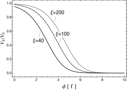
therefore the potential becomes flat at a small field limit but it has a shape of run-away potential at a large field limit as we desired. The schematic shape of the potential is shown in the Fig. 1. Clearly, our model is distinctive from the earlier attempt for scaling solution [48], and more recent model with a generalized exponential potential [49].
The slow-roll parameters are explicitly given as
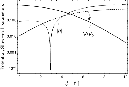
In Fig. 2 we depicted the slow-roll parameters and in different field values in a small field regime. We set and for the illustration purpose.
3 Early time inflation
In the vicinity of the origin, or , the potential becomes flat and potentially supports the early time inflation. In this regime (small-field limit), we find an approximate expression:
| (9) |
We also simplify as
The slow-roll parameters are given in the small field limit , and :
The number of e-foldings during inflation is calculated in the small field limit:
| (10) |
where is for the CMB pivot scale where .
| (11) | ||||
| (12) | ||||
| (13) |
Requesting e-foldings, we determine the inflationary predictions for the spectral index and the tensor-to-scalar ratio
| (14) |
It is noticed that these results exactly coincide with the results of the non-minimally coupled model of inflation with a general power law (See. Ref. [21] in detail.) Finally, we determine the parameter by requesting the CMB normalization condition (TT,TE,EE+lowE+lensing) [5], leads:
| (15) |
4 Late time Dark energy
In the large field limit, or , the Einstein frame becomes indistinguishable from the Jordan frame as and or . The potential is a run-away type so that the energy density will go down as time goes on:
| (16) |
Note that this is nothing but the quintessence potential considered in [50], which has been extensively studied.
The slow-roll parameters are approximately constant in this limit:
| (17) |
The slow-roll approximation is valid when . We estimate the size of the kinetic term using the slow-roll approximation
| (18) |
which leads to the equation of state as
| (19) |
Figure 3 shows the equation of state for our model under the slow-roll approximation. For comparison, we also include recent results from DESI BAO+CMB+PantheonPlus [10]. In the large limit, the predicted value approaches , consistent with the cosmological constant; however, deviations from are possible. Such deviations would serve as a distinctive signal of the quintessence field . Notably, the model remains fully compatible with recent data for .

We now discuss the trajectory of quintessence field in a large-field limit with respect to the number of e-foldings . We set the current universe by so that in an earlier time.
| (20) |
where set at an earlier moment with . The energy density of quintessence with respect to is given by
| (21) |
Finally, matching the Hubble parameter at the current Universe tells us
| (22) |
Taking with the neutrino mass scale eV and the CMB normalization condition given in Eq. (15), we read
| (23) |
5 Summary and conclusions
In this work, we have proposed a unified theoretical framework that effectively addresses both early-time inflation and late-time dark energy using a single scalar field non-minimally coupled to gravity. By employing a carefully constructed potential with dual asymptotic plateaus, we demonstrated how the model transitions seamlessly from inflationary dynamics at small field values to a quintessence-like regime at large field values.
The model achieves compatibility with current observational constraints on inflation, producing predictions for the spectral index () and tensor-to-scalar ratio () that align with Planck and BICEP/Keck data. Furthermore, the late-time dynamics naturally yield a dark energy equation of state approaching , with measurable deviations providing a potential observational signature of the underlying quintessence mechanism.
Our results highlight the potential for a single scalar field to unify the seemingly disparate phenomena of early and late cosmic acceleration within a consistent theoretical framework. This approach not only addresses the fine-tuning challenges inherent in conventional models but also opens avenues for new observational tests of scalar-field dynamics across cosmic epochs. Future work will focus on exploring the implications of this model in varying cosmological scenarios and its sensitivity to alternative formulations of gravity.
Finally, we comment on the cosmological constant problem. Within our framework, the problem can be reformulated as . This condition can be satisfied by assuming a large field value for , specifically .
Acknowledgements
I am deeply grateful to Yi-fu Cai and Masahide Yamaguchi for their inspiring discussions. This work was supported by the National Research Foundation of Korea (NRF) grants funded by the Korean government (MSIT) under project numbers RS-2023-00283129 and RS-2024-00340153.
References
- [1] Alexei A. Starobinsky. A New Type of Isotropic Cosmological Models Without Singularity. Phys. Lett. B, 91:99–102, 1980.
- [2] Alan H. Guth. The Inflationary Universe: A Possible Solution to the Horizon and Flatness Problems. Phys. Rev. D, 23:347–356, 1981.
- [3] Katsuhiko Sato. First-order phase transition of a vacuum and the expansion of the Universe. Mon. Not. Roy. Astron. Soc., 195(3):467–479, 1981.
- [4] Andrei D. Linde. Chaotic Inflation. Phys. Lett. B, 129:177–181, 1983.
- [5] Y. Akrami et al. Planck 2018 results. X. Constraints on inflation. Astron. Astrophys., 641:A10, 2020.
- [6] P. A. R. Ade et al. Improved Constraints on Primordial Gravitational Waves using Planck, WMAP, and BICEP/Keck Observations through the 2018 Observing Season. Phys. Rev. Lett., 127(15):151301, 2021.
- [7] Adam G. Riess et al. Observational evidence from supernovae for an accelerating universe and a cosmological constant. Astron. J., 116:1009–1038, 1998.
- [8] S. Perlmutter et al. Measurements of and from 42 High Redshift Supernovae. Astrophys. J., 517:565–586, 1999.
- [9] Scott F. Daniel, Robert R. Caldwell, Asantha Cooray, and Alessandro Melchiorri. Large Scale Structure as a Probe of Gravitational Slip. Phys. Rev. D, 77:103513, 2008.
- [10] A. G. Adame et al. DESI 2024 VI: Cosmological Constraints from the Measurements of Baryon Acoustic Oscillations. 4 2024.
- [11] Yi-Fu Cai, Emmanuel N. Saridakis, Mohammad R. Setare, and Jun-Qing Xia. Quintom Cosmology: Theoretical implications and observations. Phys. Rept., 493:1–60, 2010.
- [12] Miao Li, Xiao-Dong Li, Shuang Wang, and Yi Wang. Dark Energy. Commun. Theor. Phys., 56:525–604, 2011.
- [13] Kazuharu Bamba, Salvatore Capozziello, Shin’ichi Nojiri, and Sergei D. Odintsov. Dark energy cosmology: the equivalent description via different theoretical models and cosmography tests. Astrophys. Space Sci., 342:155–228, 2012.
- [14] Shinji Tsujikawa. Quintessence: A Review. Class. Quant. Grav., 30:214003, 2013.
- [15] P. J. E. Peebles and A. Vilenkin. Quintessential inflation. Phys. Rev. D, 59:063505, 1999.
- [16] Jean-Philippe Uzan. Cosmological scaling solutions of nonminimally coupled scalar fields. Phys. Rev. D, 59:123510, 1999.
- [17] Yi-Fu Cai, Jie Liu, and Hong Li. Entropic cosmology: a unified model of inflation and late-time acceleration. Phys. Lett. B, 690:213–219, 2010.
- [18] Yi-Fu Cai and Emmanuel N. Saridakis. Inflation in Entropic Cosmology: Primordial Perturbations and non-Gaussianities. Phys. Lett. B, 697:280–287, 2011.
- [19] Jaume de Haro and Llibert Aresté Saló. A Review of Quintessential Inflation. Galaxies, 9(4):73, 2021.
- [20] T. Futamase and Kei-ichi Maeda. Chaotic Inflationary Scenario in Models Having Nonminimal Coupling With Curvature. Phys. Rev. D, 39:399–404, 1989.
- [21] Seong Chan Park and Satoshi Yamaguchi. Inflation by non-minimal coupling. JCAP, 08:009, 2008.
- [22] Renata Kallosh and Andrei Linde. Universality Class in Conformal Inflation. JCAP, 07:002, 2013.
- [23] Renata Kallosh, Andrei Linde, and Diederik Roest. Superconformal Inflationary -Attractors. JHEP, 11:198, 2013.
- [24] Dhong Yeon Cheong, Hyun Min Lee, and Seong Chan Park. Beyond the Starobinsky model for inflation. Phys. Lett. B, 805:135453, 2020.
- [25] Ryusuke Jinno, Kunio Kaneta, Kin-ya Oda, and Seong Chan Park. Hillclimbing inflation in metric and Palatini formulations. Phys. Lett. B, 791:396–402, 2019.
- [26] Sang Chul Hyun, Jinsu Kim, Seong Chan Park, and Tomo Takahashi. Non-minimally assisted chaotic inflation. JCAP, 05(05):045, 2022.
- [27] Sang Chul Hyun, Jinsu Kim, Tatsuki Kodama, Seong Chan Park, and Tomo Takahashi. Nonminimally assisted inflation: a general analysis. JCAP, 05:050, 2023.
- [28] Seoktae Koh, Seong Chan Park, and Gansukh Tumurtushaa. Higgs inflation with a Gauss-Bonnet term. Phys. Rev. D, 110(2):023523, 2024.
- [29] Yongsoo Jho, Tae-Geun Kim, Jong-Chul Park, Seong Chan Park, and Yeji Park. Axions from Primordial Black Holes. 12 2022.
- [30] Dhong Yeon Cheong, Seong Chan Park, and Chang Sub Shin. Effective theory approach for axion wormholes. JHEP, 07:039, 2024.
- [31] Dhong Yeon Cheong, Koichi Hamaguchi, Yoshiki Kanazawa, Sung Mook Lee, Natsumi Nagata, and Seong Chan Park. Axion quality problem and nonminimal gravitational coupling in the Palatini formulation. Phys. Rev. D, 108(1):015007, 2023.
- [32] Dhong Yeon Cheong, Koichi Hamaguchi, Yoshiki Kanazawa, Sung Mook Lee, Natsumi Nagata, and Seong Chan Park. Wormhole-Induced ALP Dark Matter. 11 2024.
- [33] Fedor L. Bezrukov and Mikhail Shaposhnikov. The Standard Model Higgs boson as the inflaton. Phys. Lett. B, 659:703–706, 2008.
- [34] Yuta Hamada, Hikaru Kawai, Kin-ya Oda, and Seong Chan Park. Higgs inflation from Standard Model criticality. Phys. Rev. D, 91:053008, 2015.
- [35] Yuta Hamada, Hikaru Kawai, Kin-ya Oda, and Seong Chan Park. Higgs Inflation is Still Alive after the Results from BICEP2. Phys. Rev. Lett., 112(24):241301, 2014.
- [36] Yohei Ema. Higgs Scalaron Mixed Inflation. Phys. Lett. B, 770:403–411, 2017.
- [37] Dmitry Gorbunov and Anna Tokareva. Scalaron the healer: removing the strong-coupling in the Higgs- and Higgs-dilaton inflations. Phys. Lett. B, 788:37–41, 2019.
- [38] Anirudh Gundhi and Christian F. Steinwachs. Scalaron-Higgs inflation. Nucl. Phys. B, 954:114989, 2020.
- [39] Minxi He, Ryusuke Jinno, Kohei Kamada, Seong Chan Park, Alexei A. Starobinsky, and Jun’ichi Yokoyama. On the violent preheating in the mixed Higgs- inflationary model. Phys. Lett. B, 791:36–42, 2019.
- [40] Dhong Yeon Cheong, Sung Mook Lee, and Seong Chan Park. Primordial black holes in Higgs- inflation as the whole of dark matter. JCAP, 01:032, 2021.
- [41] Dhong Yeon Cheong, Kazunori Kohri, and Seong Chan Park. The inflaton that could: primordial black holes and second order gravitational waves from tachyonic instability induced in Higgs-R 2 inflation. JCAP, 10:015, 2022.
- [42] Dhong Yeon Cheong, Sung Mook Lee, and Seong Chan Park. Progress in Higgs inflation. J. Korean Phys. Soc., 78(10):897–906, 2021.
- [43] F. Lucchin and S. Matarrese. Power Law Inflation. Phys. Rev. D, 32:1316, 1985.
- [44] J. J. Halliwell. Scalar Fields in Cosmology with an Exponential Potential. Phys. Lett. B, 185:341, 1987.
- [45] A. B. Burd and John D. Barrow. Inflationary Models with Exponential Potentials. Nucl. Phys. B, 308:929–945, 1988. [Erratum: Nucl.Phys.B 324, 276–276 (1989)].
- [46] Ryusuke Jinno, Mio Kubota, Kin-ya Oda, and Seong Chan Park. Higgs inflation in metric and Palatini formalisms: Required suppression of higher dimensional operators. JCAP, 03:063, 2020.
- [47] Dhong Yeon Cheong, Sung Mook Lee, and Seong Chan Park. Reheating in models with non-minimal coupling in metric and Palatini formalisms. JCAP, 02(02):029, 2022.
- [48] Andrew R. Liddle and Robert J. Scherrer. A Classification of scalar field potentials with cosmological scaling solutions. Phys. Rev. D, 59:023509, 1999.
- [49] Chao-Qiang Geng, Chung-Chi Lee, M. Sami, Emmanuel N. Saridakis, and Alexei A. Starobinsky. Observational constraints on successful model of quintessential Inflation. JCAP, 06:011, 2017.
- [50] T. Barreiro, Edmund J. Copeland, and N. J. Nunes. Quintessence arising from exponential potentials. Phys. Rev. D, 61:127301, 2000.