Panel Stochastic Frontier Models with Latent Group Structures

Abstract

Stochastic frontier models have attracted significant interest over the years due to their unique feature of including a distinct inefficiency term alongside the usual error term. To effectively separate these two components, strong distributional assumptions are often necessary. To overcome this limitation, numerous studies have sought to relax or generalize these models for more robust estimation. In line with these efforts, we introduce a latent group structure that accommodates heterogeneity across firms, addressing not only the stochastic frontiers but also the distribution of the inefficiency term. This framework accounts for the distinctive features of stochastic frontier models, and we propose a practical estimation procedure to implement it. Simulation studies demonstrate the strong performance of our proposed method, which is further illustrated through an application to study the cost efficiency of the U.S. commercial banking sector.

Keywords:

Classification, Group Structures, Panel Data, Stochastic Frontier

JEL classification:

C23, C33, C38, C51

1 Introduction

Aigner et al. (1977) and Meeusen and van Den Broeck (1977) introduced the stochastic frontier (SF) model to study the productive (in)efficiency of firms. Such SF models have gained considerable attention ever since. We refer readers to Kumbhakar and Lovell (2000) for early developments and Kumbhakar et al. (2022) and Tsionas et al. (2023) for recent advancements and a comprehensive review of the literature. One distinct feature of a SF model is the decomposition of the error term, which is typically expressed as $\varepsilon=v-u$, where $v$ represents a random disturbance and $u$ is the inefficiency term, with $u\geq 0$. Unlike standard regression models, the identification of $v$ and $u$ is crucial in SF modeling due to their economic interpretations. Separate identification of $v$ and $u$ usually requires imposing strong distributional assumptions.

We consider the following heterogeneous time-varying panel stochastic frontier (SF) model:

$$y_{it} =\alpha_{i}^{0}+\alpha_{i}(\tau_{t})+x_{it}^{\prime}\beta_{i}(\tau_{t})+\varepsilon_{it},\quad\text{with}\quad\varepsilon_{it}=v_{it}-u_{i},$$

$$=\alpha_{i}^{0}-u_{i}+\alpha_{i}(\tau_{t})+x_{it}^{\prime}\beta_{i}(\tau_{t})+v_{it},$$

for firm $i=1,2,\dots,N$ and time $t=1,2,\dots,T$, and $\tau_{t}=t/T\in(0,1]$. In this model, $\alpha_{i}^{0}$ and $\alpha_{i}(\tau_{t})$ denote the constant and time-varying intercepts of the efficient frontier, respectively. The time-varying intercept $\alpha_{i}(\tau_{t})$ is normalized such that $\int_{0}^{1}\alpha_{i}(\tau_{t})\,d\tau_{t}=1$, ensuring that $\alpha_{i}^{0}$ is identifiable. The term $\beta_{i}(\tau_{t})$ denotes a non-random, time-varying coefficient vector. The error term $v_{it}$ is a random variable with zero mean, and $u_{i}\geq 0$ represents the firm-specific random inefficiency term. In addition to allowing for heterogeneity in the efficient frontier, we also allow the variance of $v_{it}$ to vary across firms, as well as to account for the possibility that $u_{i}$ is generated from different distributions. The model is robust with respect to the aforementioned sources of heterogeneity stemming from both the frontier and the inefficiency term.

Our study is motivated by heterogeneity, which can either shift the efficiency frontier or distort the location and scale of inefficiency estimates (see, for example, Galan et al., 2014). According to Greene (2005a), the true underlying frontier might include unmeasured firm-specific characteristics that reflect the technology in use. Greene (2005a) was instrumental in expanding stochastic frontier models to incorporate firm heterogeneity by allowing for either true fixed effects or true random effects. Building on this, heterogeneity was further explored by allowing the inefficiency term to be either purely transient or a combination of transient and persistent (see, for example Colombi et al., 2014; Kumbhakar et al., 2014; Tsionas and Kumbhakar, 2014). These approaches enable unobserved heterogeneity across individuals to be separated from inefficiency effects.

We aim to present a new framework by incorporating heterogeneity across firms in both frontiers and composite error distributions. We assume a latent group structure that mitigates overfitting issues. Specifically, we assume there are $K^{*}\geq 1$ groups. All firms within each group share the same set of parameters $\left\{\alpha(\tau_{t}),\beta(\tau_{t}),\text{var}(v_{t})\right\}$. Importantly, we do not impose the same group structure for the distribution of the inefficiency term $(u)$ along with the constant term $\alpha^{0}$. We find that defining group membership for $(\alpha^{0},u)$ in the same way as for the others is inappropriate, as discussed in detail in Section 2.4. We account for potential structure in $\alpha^{0}-u$ by modeling it as a mixture of two different distributions.

The concept of uncovering latent group structures within panel data models has been extensively studied in recent years. Broadly, these methods can be categorized into two main approaches. One approach uses K-means clustering based on individual-level estimations, with notable contributions from Lin and Ng (2012), Bonhomme and Manresa (2015), Ando and Bai (2016), and Chen (2019). The second approach, which was introduced by Su et al. (2016), incorporated an innovative penalty function applied to joint mean squared errors, allowing for simultaneous estimation and classification. Further advancements in this approach are found in Su et al. (2019), Huang et al. (2020) and Wang and Su (2021), just to name a few. Conceptually, the latter approach pools all observations across firms for joint estimation and classification, whereas the former relies on individual (non-pooled) firm-level estimations for classification.

Existing approaches cannot be directly applied here due to the following reasons. Estimating parameters that describe the underlying distribution of $u_{i}$ requires pooling the observations across firms. Typically, this pooling-based estimation is conducted using maximum likelihood estimation (MLE) for the likelihood function in (A.2). However, the log-likelihood function is complex and highly nonlinear, making numerical optimization difficult when numerous unknown parameters are involved, as required for joint estimation in Su et al. (2016). This leads to a dilemma. To address this, we propose a new practical approach that combines pooled and non-pooled estimation methods.

Our paper makes several contributions to the literature on SF models and classification methods for panel data models. First, we estimate a robust panel SF model by incorporating heterogeneity across firms. We carefully define the framework, clarifying feasible and infeasible approaches with detailed explanations of the underlying reasons. Second, to the best of our knowledge, this paper is among the few that model and allow error terms to exhibit latent structures. A notable study in this area was by Loyo and Boot (2024), which focused on modeling error term variance primarily for efficiency or specific roles of variance. In contrast, we consider not only the variance of $v$ but also the entire distribution of $u$. Given the importance of modeling both the variance of $v$ and the distribution of $u$ in SF models, we view this as a substantial contribution. Finally, to address heterogeneity arising from both the frontier and error terms, we propose an estimation procedure that combines individual-level and joint panel estimation, providing justification for the necessity of this approach.

The rest of this paper is organized as follows. In Section 2, we introduce the estimation procedure and propose information criteria to determine the number of groups and whether $u$ follows a unique or mixed distribution. Section 3 examines the theoretical properties of our procedure, specifying the conditions required for tuning parameters. In Section 4, we evaluate the small-sample performance of our method, providing practical recommendations for tuning parameters that meet the conditions and perform well in simulations. In Section 5, we apply our procedure to a dataset of large U.S. commercial banks, using the recommended tuning parameters from the simulations. Our findings confirm the presence of heterogeneity in frontiers and a mixture distribution for the inefficiency term. Appendix A and B describe, respectively, the approximate likelihood function of the model and the clustering method used. Proofs of the theorems and propositions from Section 3 are provided in Appendix C, with technical lemmas presented in Appendix F. Additional simulation and application results are included in Appendix  D, and Appendix E further discusses the properties of the information matrix in support of Appendix C.

2 Model and Estimation

This section presents the model and the estimation procedure. To ease exposition, we assume $\alpha_{i}^{0}=\alpha^{0}$ and $\text{var}(u_{i})=\sigma_{u}^{2}$ for all $i$ in Sections 2.1 to 2.3. These restrictions are relaxed to the general case afterward. All technical conditions, theoretical properties, and the main theorems are deferred to the next section.

2.1 The Model

We analyze panel stochastic frontier models with random fixed effects. Our model extends Yao et al. (2019) by incorporating heterogeneous, time-varying coefficients:

$$y_{it} =\alpha^{0}+\alpha_{i}\left(\tau_{t}\right)+x_{it}^{\prime}\beta_{i}\left(\tau_{t}\right)+\varepsilon_{it}$$

$$=\alpha^{0}-u_{i}+\alpha_{i}\left(\tau_{t}\right)+\sum_{l=1}^{p}x_{itl}\beta_{il}\left(\tau_{t}\right)+v_{it},$$ (2.1)

To aid exposition, we temporarily restrict $\alpha^{0}_{i}=\alpha^{0}$, deviating from the more general case discussed in the Introduction. The subscript $l$ denotes the $l$-th element of a vector, and $x_{it}$ is $p$ by 1. In this specification, $\varepsilon_{it}=v_{it}-u_{i}$, where $v_{it}$ is a mean-zero random error term, and $u_{i}$ is a non-negative term capturing the inefficiency of firm $i$. To identify $\alpha^{0}$ and $\alpha_{i}\left(\tau_{t}\right)$, we adopt the normalization

$$\int_{0}^{1}\alpha_{i}(s)\,ds=0,$$

which is standard in the literature (e.g., Atak et al. (2023)). This normalization ensures that $\alpha_{i}(s)$ captures the time-varying component of the intercept term. When the intercept term is not time-varying, $\alpha_{i}(s)=0$.

As in Yao et al. (2019), we assume that

$$v_{it}\sim N(0,\sigma_{vi}^{2}),u_{i}\sim|N(0,\sigma_{u}^{2})|,\text{ and }v_{it}\perp u_{i}\perp x_{it}.$$

Unlike in the Introduction, we assume here $\sigma_{u}^{2}$ are identical for all $i$ (no group structure) for now. These two parameters ($\alpha^{0}$ and $\sigma_{u}^{2}$) exhibit unique features compared to other parameters. We defer discussions to Section 2.4 for better exposition.

We assume there are $K^{\ast}$ groups of specific parameters, and each firm’s parameters belong to one of these groups. Mathematically,

$$\left\{\alpha_{i}\left(\tau_{t}\right),\beta_{i}\left(\tau_{t}\right),\sigma_{vi}\right\}=\sum_{k=1}^{K^{\ast}}\left\{\alpha_{(k)}^{\ast}\left(\tau_{t}\right),\beta_{(k)}^{\ast}\left(\tau_{t}\right),\sigma_{v(k)}^{\ast}\right\}\boldsymbol{1}(i\in G_{k}),$$ (2.2)

where $\boldsymbol{1}(\cdot)$ is the indicator function, equaling 1 if $\cdot$ is true and 0 otherwise. We assume that parameters from different groups are distinct, meaning

$$\left\{\alpha_{(k)}^{\ast}\left(\tau_{t}\right),\beta_{(k)}^{\ast}\left(\tau_{t}\right),\sigma_{v(k)}^{\ast}\right\}\neq\left\{\alpha_{(j)}^{\ast}\left(\tau_{t}\right),\beta_{(j)}^{\ast}\left(\tau_{t}\right),\sigma_{v(j)}^{\ast}\right\},$$

for $j\neq k$. The group membership sets satisfy

$$G_{j}\cap G_{k}=\emptyset\text{ and }\bigcup_{k=1}^{K^{\ast}}G_{k}=\left\{1,2,\dots,N\right\}.$$

In simpler terms, this setup means that each firm’s parameters uniquely belong to one of the $K^{\ast}$ groups.

We adopt this setup primarily to illustrate our approach. Readers can generalize the methodology presented here to other model specifications, such as the four-component panel stochastic frontier model discussed in Lai and Kumbhakar (2023).

2.2 Approximation of $\alpha\left(\cdot\right)$ and $\beta\left(\cdot\right)$

The approximations we adopt are standard in the literature. Let $L^{2}\left[0,1\right]=\{f\left(s\right):\int_{0}^{1}f^{2}\left(s\right)ds<\infty\}$ represent the space of square-integrable functions. In this space, the inner product is defined as $\left\langle f_{1},f_{2}\right\rangle\equiv\int_{0}^{1}f_{1}\left(s\right)f_{2}\left(s\right)ds$, and the induced norm is $\left\|f\right\|=\left\langle f,f\right\rangle^{1/2}$. Following Dong and Linton (2018), we use cosine functions as basis functions: $B_{0}\left(s\right)=1$ and $B_{j}\left(s\right)=\sqrt{2}\cos(j\pi s)$ for $j\geq 1$. The set $\{B_{j}\left(s\right)\}_{j=0}^{\infty}$ forms an orthonormal basis for the Hilbert space $L^{2}\left[0,1\right]$, such that $\left\langle B_{i},B_{j}\right\rangle=\delta_{ij}$, where $\delta_{ij}$ is the Kronecker delta, which equals 1 if $i=j$, and 0 otherwise.

Suppose $f(\cdot)\in L^{2}\left[0,1\right]$ is $\kappa$-th order continuously differentiable, then we have

$$f\left(s\right) =\sum_{j=0}^{\infty}B_{j}\left(s\right)v_{j}^{0}=\sum_{j=0}^{m-1}B_{j}\left(s\right)v_{j}^{0}+\sum_{j=m}^{\infty}B_{j}\left(s\right)v_{j}^{0}$$

$$=\sum_{j=0}^{m-1}B_{j}\left(s\right)v_{j}^{0}+O\left(m^{-\kappa}\right)\equiv\mathbb{B}^{m}\left(s\right)^{\prime}v^{0}+O\left(m^{-\kappa}\right),$$

where $\mathbb{B}^{m}\left(s\right)\equiv\left(B_{0}\left(s\right),B_{1}\left(s\right),\dots,B_{m-1}\left(s\right)\right)^{\prime}$, $v_{j}^{0}=\left\langle f,B_{j}\right\rangle$, and $v^{0}=\left(v_{0}^{0},v_{1}^{0},\dots,v_{m-1}^{0}\right)^{\prime}$. Here, $\sum_{j=m}^{\infty}B_{j}\left(s\right)v_{j}^{0}$ is the bias term from using only $\mathbb{B}^{m}\left(s\right)$ to approximate $f\left(s\right)$. If $f\left(s\right)$ is $\kappa$-th order differentiable, the bias term $\sum_{j=m}^{\infty}B_{j}\left(s\right)v_{j}^{0}=O\left(m^{-\kappa}\right)$. For $f$ when $\int_{0}^{1}f\left(s\right)ds=0$ is imposed, we approximate $f$ by using $\mathbb{B}_{-0}^{m}\left(s\right)\equiv\left(B_{1}\left(s\right),\dots,B_{m-1}\left(s\right)\right)^{\prime}$, since $\int_{0}^{1}B_{j}\left(s\right)ds=0$ for $j\geq 1$. Similarly,

$$f\left(s\right)=\mathbb{B}_{-0}^{m}\left(s\right)v_{-0}^{0}+O\left(m^{-\kappa}\right),$$

for some $v_{-0}^{0}=\left(v_{1}^{0},v_{2}^{0},\dots,v_{m-1}^{0}\right)^{\prime}$.

We apply this approximation to our case. For each firm $i$, we have

$$y_{it} =\alpha^{0}-u_{i}+\alpha_{i}\left(\tau_{t}\right)+\sum_{l=1}^{p}x_{itl}\beta_{il}\left(\tau_{t}\right)+v_{it}$$

$$\approx\alpha^{0}-u_{i}+\mathbb{B}_{-0}^{m}\left(\tau_{t}\right)^{\prime}\pi_{i0}^{0}+\sum_{l=1}^{p}x_{itl}\mathbb{B}^{m}\left(\tau_{t}\right)^{\prime}\pi_{il}^{0}+v_{it}$$

$$\equiv\alpha^{0}-u_{i}+\left[\mathbb{B}_{-0}^{m}\left(\tau_{t}\right)^{\prime},\left(x_{it}\otimes\mathbb{B}^{m}\left(\tau_{t}\right)\right)^{\prime}\right]\pi_{i}^{0}+v_{it}$$

$$\equiv\alpha^{0}-u_{i}+z_{it}^{\prime}\pi_{i}^{0}+v_{it}\equiv\tilde{z}_{it}^{\prime}\tilde{\pi}_{i}^{0}+v_{it},$$ (2.3)

where the terms $\mathbb{B}_{-0}^{m}\left(\tau_{t}\right)^{\prime}\pi_{i0}^{0}$ and $\mathbb{B}^{m}\left(\tau_{t}\right)^{\prime}\pi_{il}^{0}$ represent approximations of $\alpha_{i}\left(\tau_{t}\right)$ and $\beta_{il}\left(\tau_{t}\right)$, respectively, and

$$x_{it}\otimes\mathbb{B}^{m}\left(\tau_{t}\right) \equiv\left(x_{it1}B_{0}\left(\tau_{t}\right),\dots,x_{it1}B_{m-1}\left(\tau_{t}\right),\dots,x_{itp}B_{0}\left(\tau_{t}\right),\dots,x_{itp}B_{m-1}\left(\tau_{t}\right)\right)^{\prime},$$

$$\pi_{i}^{0} \equiv\left(\pi_{i0}^{0\prime},\pi_{i1}^{0\prime},\dots,\pi_{ip}^{0\prime}\right)^{\prime},\quad\tilde{\pi}_{i}^{0}\equiv\left(\alpha^{0}-u_{i},\pi_{i0}^{0\prime},\pi_{i1}^{0\prime},\dots,\pi_{ip}^{0\prime}\right)^{\prime},$$

$$z_{it} \equiv\left[\mathbb{B}_{-0}^{m}\left(\tau_{t}\right)^{\prime},\left(x_{it}\otimes\mathbb{B}^{m}\left(\tau_{t}\right)\right)^{\prime}\right]^{\prime},\quad\text{and}\quad\tilde{z}_{it}\equiv\left(1,z_{it}^{\prime}\right)^{\prime}.$$

The last two lines of equation (2.3) represent three equivalent ways of expressing the approximation.

2.3 The Estimation

Stochastic frontier models exhibit distinctive characteristics compared to standard panel data models. Notably, the intercept term $\alpha^{0}-u_{i}$, which is typically insignificant in standard panel models, becomes a key parameter of interest in stochastic frontier models. Furthermore, the variance component $\sigma_{u}^{2}$ is identified through the skewness in the distribution of $\alpha^{0}-u_{i}$ across $i$. As a result, $\sigma_{u}^{2}$ cannot be identified or estimated without pooling observations across different $i$.

However, pooling observations for estimation introduces challenges. Specifically, the log-likelihood functions in (A.2) and (A.3) are highly nonlinear, leading to difficulties in numerical optimization, especially when numerous unknown parameters are involved. This issue becomes particularly pronounced in pooled estimation with classification methods, such as those proposed by Su et al. (2016). This creates a dilemma regarding whether to pool observations for estimation.

To address these challenges, we propose a procedure that combines estimations with and without pooling. Initially, we omit the estimation of $\sigma_{u}^{2}$ and estimate $(\pi_{i}^{0\prime},\sigma_{vi})^{\prime}$ for each $i$ using the Ordinary Least Squares (OLS) estimator. Next, we classify observations into groups based on estimates of $\vartheta_{i}\equiv(\pi_{i}^{0\prime},\sigma_{vi})^{\prime}$, employing a K-means clustering algorithm. Notably, since $\alpha^{0}-u_{i}$ naturally varies across $i$, classification is based only on $\vartheta_{i}$, excluding the intercept term. In the third step, we determine the number of groups using an information criterion and obtain post-classification frontier estimates. In Step 4, we pool observations post-classification to estimate $\alpha^{0}$ and $\sigma_{u}^{2}$ using the results from Step 3.

The detailed steps of this procedure are presented below.

Step 1: Individual Estimation

Using the approximation from (2.3), we regress $y_{it}$ against $\mathbb{B}^{m}\left(\tau_{t}\right)$ and $x_{it}\otimes\mathbb{B}^{m}\left(\tau_{t}\right)$ for $t=1,2,\ldots,T$ to obtain $\widehat{\tilde{\pi}}_{i}$. From this we obtain $\hat{\sigma}_{vi}^{2}$ as the sample variance of the regression residuals.

Specifically, consider the following expression:

$$Z_{im}\equiv\left(\begin{array}[]{c}\tilde{z}_{i1}^{\prime}\\ \vdots\\ \tilde{z}_{iT}^{\prime}\end{array}\right)_{T\times m(p+1)}.$$

Then the OLS estimator for firm $i$ is given by

$$\widehat{\tilde{\pi}}_{i}=\left(Z_{im}^{\prime}Z_{im}\right)^{-1}Z_{im}^{\prime}y_{i},$$ (2.4)

with $y_{i}=\left(y_{i1},\ldots,y_{iT}\right)^{\prime}$. We then obtain $\hat{\sigma}_{vi}^{2}$ as follows:

$$\hat{\sigma}_{vi}^{2}=\frac{1}{T-1}\sum_{t=1}^{T}\left(y_{it}-\tilde{z}_{it}^{\prime}\widehat{\tilde{\pi}}_{i}\right)^{2}.$$

Excluding the first element in $\widehat{\tilde{\pi}}_{i}$, we let $\hat{\pi}_{i}$ denote the estimated coefficients associated with $z_{it}$. We collect the estimates $\hat{\pi}_{i}$ and $\hat{\sigma}_{vi}$ to form an estimate of $\vartheta_{i}$:

$$\hat{\vartheta}_{i}=\left(\hat{\pi}_{i}^{\prime},\hat{\sigma}_{vi}\right)^{\prime},$$

based on which we form groups.

Step 2: Classification

We obtained $\hat{\vartheta}_{1},\hat{\vartheta}_{2},\ldots,\hat{\vartheta}_{n}$ from Step 1. We use the $L_{2}$ norm to measure the distance between $\hat{\vartheta}_{i}$ and $\hat{\vartheta}_{j}$. Based on this distance measure, we then apply the classical Hierarchical Agglomerative Clustering (HAC) method to the estimates of each firm’s functional coefficient to determine group memberships. The HAC method is commonly used for clustering; for a review, we refer readers to Everitt et al. (2011). Details of the HAC method are provided in Appendix B. Given a value for $K$, we apply the HAC method to obtain an estimate of the group membership, denoted as

$$\left(\hat{G}_{1|K},\hat{G}_{2|K},\ldots,\hat{G}_{K|K}\right),$$

which forms a partition of the set $\left\{1,2,\ldots,N\right\}$.

Step 3: Post-Classification Estimation and Determination of $K^{\ast}$

Within each group, we now have significantly more observations available for pooling. Recognizing this, we set the number of sieve terms to $\underline{m}$, which is substantially larger than $m$. We define the new regressors as $\underline{z}_{it}$:

$$\underline{z}_{it}=\left[\mathbb{B}_{-0}^{\underline{m}}\left(\tau_{t}\right)^{\prime},\left(x_{it}\otimes\mathbb{B}^{\underline{m}}\left(\tau_{t}\right)\right)^{\prime}\right]^{\prime}$$

Within each group, e.g., $\hat{G}_{k|K}$ where $1\leq k\leq K$, we conduct post-classification estimation using standard within-panel data estimation methods. At this stage, we do not consider $\alpha^{0}-u_{i}$. Specifically,

$$\hat{\pi}_{(k|K)}=\arg\min_{\pi}\sum_{i\in\hat{G}_{k|K}}\sum_{t=1}^{T}\left(\ddot{y}_{it}-\underline{\ddot{z}}_{it}^{\prime}\pi\right)^{2},$$

where

$$\ddot{y}_{it}=y_{it}-\frac{1}{T}\sum_{t=1}^{T}y_{it},\quad\underline{\ddot{z}}_{it}=\underline{z}_{it}-\frac{1}{T}\sum_{t=1}^{T}\underline{z}_{it}.$$

The variance of $v_{it}$ for group $k$ is estimated as

$$\hat{\sigma}_{v(k|K)}^{2}=\frac{1}{N_{k}(T-1)}\sum_{i\in\hat{G}_{k|K}}\sum_{t=1}^{T}\left(\ddot{y}_{it}-\underline{\ddot{z}}_{it}^{\prime}\hat{\pi}_{(k|K)}\right)^{2},$$

where $N_{k}=\sharp\{\hat{G}_{k|K}\}$ is the number of elements in $\hat{G}_{k|K}$. For simplicity, we do not explicitly distinguish between $\hat{N}_{k}=\sharp\{\hat{G}_{k|K^{*}}\}$ and $N_{k}=\sharp\{G_{k|K^{*}}\}$. Similarly,

$$\hat{\vartheta}_{(k|K)}=\left(\hat{\pi}_{(k|K)}^{\prime},\hat{\sigma}_{v(k|K)}\right)^{\prime}.$$

Inspired by the pseudo-loglikelihood, we construct an information criterion to determine the number of groups as follows:

$$\text{IC}(K,\lambda_{NT}) =\sum_{k=1}^{K}\left\{N_{k}T\log(\hat{\sigma}_{v(k|K)})+\sum_{i\in\hat{G}_{k|K}}\sum_{t=1}^{T}\frac{\left(\ddot{y}_{it}-\underline{\ddot{z}}_{it}^{\prime}\hat{\pi}_{(k|K)}\right)^{2}}{\hat{\sigma}_{v(k|K)}^{2}}\right\}+\lambda_{NT}K,$$

$$=\sum_{k=1}^{K}\left\{N_{k}T\log(\hat{\sigma}_{v(k|K)})+N_{k}(T-1)\right\}+\lambda_{NT}K,$$ (2.5)

where $\lambda_{NT}$ is a suitable penalty term. We determine the optimal number of groups as

$$\hat{K}(\lambda_{NT})=\arg\min_{K=0,1,\ldots,\bar{K}}\text{IC}(K,\lambda_{NT}),$$

for a suitable $\bar{K}$. For brevity, we refer to this simply as $\hat{K}$. Our final estimates are then given by

$$\hat{\vartheta}_{(k|\hat{K})}=\left(\hat{\pi}_{(k|\hat{K})},\hat{\sigma}_{v(k|\hat{K})}\right),\quad k=1,2,\ldots,\hat{K}.$$

Step 4: Estimation of $\alpha^{0}$ and $\sigma_{u}^{2}$

We estimate $\alpha^{0}$ and $\sigma_{u}^{2}$ using all observations via MLE. Specifically, the estimation is given by

$$\left(\hat{\alpha}^{0},\hat{\sigma}_{u}^{2}\right)=\arg\max_{(s,\delta_{u}^{2})}\sum_{k=1}^{\hat{K}}\sum_{i\in\hat{G}_{k|\hat{K}}}\log f\left(y_{i}\mid x_{i};s,\delta_{u}^{2},\hat{\vartheta}_{(k|\hat{K})}\right),$$

where $y_{i}=\left(y_{i1},\ldots,y_{iT}\right)^{\prime}$, $x_{i}=\left(x_{i1},\ldots,x_{iT}\right)^{\prime}$, and $f\left(y_{i}\mid x_{i};s,\delta_{u}^{2},\hat{\vartheta}_{(k|\hat{K})}\right)$ is defined in (A.2), and we use the post-classification estimates of $\vartheta$. Since only two parameters, $\alpha^{0}$ and $\sigma_{u}^{2}$, are being estimated at this stage, the numerical optimization is straightforward.

2.4 Inefficiency Term

We now consider the general case where $\alpha^{0}$ can be heterogeneous across $i$, and we will use $\alpha^{0}_{i}$ from this point onward. Modeling the underlying structure of $\alpha^{0}_{i}-u_{i}$ differs from that of $\left(\alpha_{i}\left(\tau_{t}\right),\beta_{i}\left(\tau_{t}\right),\sigma_{vi}^{2}\right)$ because $u_{i}$ is assumed to be a random effect, and $\alpha^{0}_{i}-u_{i}$ naturally varies across $i$, even when $\alpha^{0}_{i}$ is identical. For this reason, we focus on identifying the distribution of $\alpha^{0}_{i}-u_{i}$ rather than the actual values. While we can uncover the underlying distribution, consistently estimating group membership remains challenging.

Consider the following example to illustrate this point. Suppose we have two random variables $\varepsilon_{1}$ and $\varepsilon_{2}$, with $\varepsilon_{1}\sim 0-\left|N(0,2)\right|$ and $\varepsilon_{2}\sim 1-\left|N(0,1)\right|$. If we mix i.i.d. realizations of $\varepsilon_{1}$ and $\varepsilon_{2}$, such as $\left\{\varepsilon_{11},\varepsilon_{12},\ldots,\varepsilon_{1n},\varepsilon_{21},\varepsilon_{22},\ldots,\varepsilon_{2n}\right\}$, it is likely that many $\varepsilon_{1i}$ and $\varepsilon_{2j}$ will be very close. For example, a small-scale Monte Carlo experiment with $n=100$ suggests that about 28% of $\varepsilon_{1i}$ will have at least one $\varepsilon_{2j}$ within a radius of 0.01. In such cases, swapping their memberships would likely have minimal impact on the likelihood function, complicating their distinct identification from the data.

Misclassification of group memberships can have a serious impact on the inefficiency term, unlike parameters at the frontiers, where only similar frontiers can be misclassified together due to low power or minor estimation errors. Continuing the previous example, suppose $\varepsilon_{1i}=0$ (highly efficient with $u_{1i}=0$) was misclassified as $\varepsilon_{2}$, then the inefficiency term for $\varepsilon_{1i}$ would be calculated as 1 (indicating inefficiency). Conversely, if $\varepsilon_{2j}=0$ (originally not efficient with $u_{2j}=1$) was misclassified as $\varepsilon_{1}$, then the inefficiency term for $\varepsilon_{2j}$ would be calculated as 0 (indicating high efficiency).

Given these challenges and the serious implications of misclassification, we adopt a mixture distribution approach as follows.

Specifically, we model $\alpha^{0}_{i}-u_{i}$ such that, with probability $\tau^{0}$, it is distributed as $\alpha^{0}_{1}-\left|N(0,\sigma_{u1}^{2})\right|$ and with probability $1-\tau^{0}$, as $\alpha^{0}_{2}-\left|N(0,\sigma_{u2}^{2})\right|$, for some $0<\tau^{0}<1$. This model enables us to uncover the structure of the $\alpha^{0}_{i}-u_{i}$ distribution through the likelihood function, estimated via MLE. This strategy is consistent with existing literature, for instance, Greene (2005b). While this model can be extended to handle more than two distributions, we focus on the simpler case of two distributions, particularly for scenarios with moderate $N$, as considered in the application of this paper.

The potential presence of a mixture distribution significantly alters the interpretation of the results. With a unique distribution, we can consistently estimate $\widehat{\alpha^{0}-u_{i}}$ as $T\to\infty$, allowing us to rank firms by efficiency because $\alpha^{0}$ is identical across $i$. However, in the case of a mixture distribution, while we can still consistently estimate $\widehat{\alpha^{0}_{i}-u_{i}}$, it is not possible to rank firms as in the former scenario. This limitation arises because group memberships—or equivalently, the values of $\alpha^{0}_{i}$—cannot be identified. This observation aligns with the findings for the cross-sectional case discussed in Greene (2005b).

The presence of a mixture structure in the distribution of $\alpha^{0}_{i}-u_{i}$ does not impact the estimation of $\vartheta_{i}$ due to the independence among $u_{i}$, $v_{it}$, and $x_{it}$. Consequently, Steps 1, 2, and 3 remain unchanged. Details of the revised Step 4, now referred to as Step 4’, are provided below.

Step 4’: Estimation of $\alpha^{0}_{1},\sigma_{u1}^{2},\alpha^{0}_{2},\sigma_{u2}^{2},\text{ and }\tau^{0}$

We adopt the mixture distribution structure for $\alpha^{0}_{i}-u_{i}$ as previously described. Using MLE, we obtain an estimate of $(\alpha^{0}_{1},\sigma_{u1}^{2},\alpha^{0}_{2},\sigma_{u2}^{2},\tau^{0})$ as follows:

$$(\hat{\alpha}^{0}_{1},\hat{\sigma}_{u1}^{2},\hat{\alpha}^{0}_{2},\hat{\sigma}_{u2}^{2},\hat{\tau})=\arg\max_{(s_{1},\delta_{u1}^{2},s_{2},\delta_{u2}^{2},\tau)}\sum_{k=1}^{\hat{K}}\sum_{i\in\hat{G}_{k|\hat{K}}}\log\tilde{f}\left(y_{i}\mid x_{i};s_{1},\delta_{u1}^{2},s_{2},\delta_{u2}^{2},\tau,\hat{\vartheta}_{(k|\hat{K})}\right),$$

where $\tilde{f}$ is the likelihood function, defined in (A.3), and we incorporate estimates from Step 3, as detailed in Section 2.3.

Collecting results from Steps 4 and 4’, we proceed to Step 5 to determine the specification of $\alpha^{0}_{i}-u_{i}$.

Step 5: Determination of the Distributional Structures of the Inefficiency Term

We introduce a new information criterion for this task:

$$\widetilde{\mathrm{IC}}_{1}(\tilde{\lambda}_{NT})=-\sum_{k=1}^{\hat{K}}\sum_{i\in\hat{G}_{k|\hat{K}}}\log f\left(y_{i}\mid x_{i};\hat{\alpha}^{0},\hat{\sigma}_{u}^{2},\hat{\vartheta}_{(k|\hat{K})}\right),$$ (2.6)

and

$$\widetilde{\mathrm{IC}}_{2}(\tilde{\lambda}_{NT})=-\sum_{k=1}^{\hat{K}}\sum_{i\in\hat{G}_{k|\hat{K}}}\log\tilde{f}\left(y_{i}\mid x_{i};\hat{\alpha}^{0}_{1},\hat{\sigma}_{u1}^{2},\hat{\alpha}^{0}_{2},\hat{\sigma}_{u2}^{2},\hat{\tau},\hat{\vartheta}_{(k|\hat{K})}\right)+\tilde{\lambda}_{NT},$$ (2.7)

where $\tilde{\lambda}_{NT}$ is a suitable penalty term, and the estimates are obtained from Steps 3, 4, and 4’.

Finally, if $\widetilde{\mathrm{IC}}_{1}(\tilde{\lambda}_{NT})\leq\widetilde{\mathrm{IC}}_{2}(\tilde{\lambda}_{NT})$, we retain the model assuming that $\alpha^{0}_{i}-u_{i}$ originates from a single distribution as in Step 4 and take $(\hat{\alpha}^{0},\hat{\sigma}_{u}^{2})$ as the estimates. Conversely, if $\widetilde{\mathrm{IC}}_{2}(\tilde{\lambda}_{NT})<\widetilde{\mathrm{IC}}_{1}(\tilde{\lambda}_{NT})$, we adopt the mixture distribution model from Step 4’ and use $(\hat{\alpha}^{0}_{1},\hat{\sigma}_{u1}^{2},\hat{\alpha}^{0}_{2},\hat{\sigma}_{u2}^{2},\hat{\tau})$.

2.5 A Summary of the Estimation Procedure

We outline the estimation procedure as follows:

1. Conduct estimations of the frontiers for each firm as described in Step 1.

2. Following Step 2, apply the HAC algorithm using the individual estimations from Step 1 for $K=1,2,\ldots,\bar{K}$.

3. Use the information criterion in (2.5) from Step 3 to determine the optimal number of groups and assign group memberships. Obtain an estimate of the frontier with the determined groups.

4. Based on the group assignments from Step 3, perform joint estimation for the inefficiency term, assuming either that $\alpha^{0}_{i}-u_{i}$ follows a unique distribution (as in Step 4) or a mixture distribution (as in Step 4’).

5. Use the information criteria in (2.6) and (2.7) to determine the distribution of $\alpha^{0}_{i}-u_{i}$, as described in Step 5.

6. Collect results. The estimates of the frontiers and the distribution of the inefficiency term are derived from Steps 3 and 5, respectively.

3 Asymptotic Properties

We examine classification consistency in Section 3.1. Subsequently, we discuss the large sample properties of the post-classification estimators in Section 3.2.

3.1 Classification

We first present the technical assumptions.

Assumption 1.

The process $\{(x_{it},v_{it}),t=1,\ldots,T\}$ is strong mixing with a mixing coefficient $\alpha(j)$ that satisfies $\alpha(j)\leq C_{\alpha}\rho^{j}$ for some positive $C_{\alpha}$ and $0<\rho<1$, and this holds for $i=1,\ldots,N$.

Assumption 2.

$\max_{1\leq i\leq N,1\leq t\leq T}\mathbb{E}\|x_{it}\|^{q}\leq\bar{C}_{x}<\infty,$ and $\max_{1\leq i\leq N,1\leq t\leq T}\mathbb{E}|v_{it}|^{q}\leq\bar{C}_{v}<\infty,$ for some $q>4.$

Assumption 3.

Denote $\tilde{x}_{it}\equiv(1,x^{\prime}_{it})^{\prime}$. $\mu_{\min}$ and $\mu_{\max}$ denote the minimum and maximum eigenvalues of a matrix, respectively. The following holds,

$$0<\underline{C}_{xx}\leq\min_{1\leq i\leq N,1\leq t\leq T}\mu_{\min}[\mathbb{E}(\tilde{x}_{it}\tilde{x}_{it}^{\prime})]\leq\max_{1\leq i\leq N,1\leq t\leq T}\mu_{\max}[\mathbb{E}(\tilde{x}_{it}\tilde{x}_{it}^{\prime})]\leq\bar{C}_{xx}<\infty.$$

Assumption 4.

For $k=1,2,\ldots,K^{*}$, $\alpha_{(k)}^{*}(s)$, $\beta_{(k)1}^{*}(s)$, …, and $\beta_{(k)p}^{*}(s)$ belong to $L^{2}\left[0,1\right]$ and are $\kappa$ times continuously differentiable.

Assumption 5.

There exists a positive $\underline{C}^{*}$, such that

$$\min_{1\leq j\neq k\leq K^{*}}\left\{\|\alpha_{(j)}^{*}-\alpha_{(k)}^{*}\|+\sum_{l=1}^{p}\|\beta_{(j)l}^{*}-\beta_{(k)l}^{*}\|+|\sigma_{v(j)}^{*}-\sigma_{v(k)}^{*}|\right\}\geq\underline{C}^{*}>0,$$

and $\min_{1\leq k\leq K^{*}}\sigma_{v(k)}^{*2}>0.$

Assumption 6.

(i) $T\propto N^{C}$ for some positive $C$ as $N\rightarrow\infty,$ where the symbol $\propto$ represents a proportional relationship. (ii) $m\rightarrow\infty$ as $N,T\rightarrow\infty.$ $Nm^{q/2+2}(\log N)^{2q}/T^{q/2-1}\rightarrow 0,$ with $q$ defined in Assumption 2.

We discuss each of these conditions individually below:

Assumption 1 imposes a condition of weak dependence across $t$, noting that independence across $i$ is not required for classifications. Assumption 2 requires $X$ and $v$ have finite $q$-th moment. Assumption 3 is the classic full rank condition. Assumption 4 stipulates that the coefficients are $\kappa$-th order differentiable, a standard condition for nonparametric or semiparametric estimation. Assumption 5 requires that at least one of the coefficients, including the variance of $v$, must differ across groups.

Assumption 6 specifies that the moment conditions must be sufficiently large, or that $T$ grows fast enough. This is crucial to ensure that the error rate is sufficiently low for the uniform convergence of $\widehat{\tilde{\pi}}_{i}$ for $i=1,2,\ldots,N$. The most stringent requirements arise from the estimation of the “design” matrix $\frac{1}{T}Z_{im}^{\prime}Z_{im}$ with diverging dimensions, used in $\widehat{\tilde{\pi}}_{i}$ (see (2.4)). For further details on this point, we refer readers to Lemma F.3, with a similar condition imposed in Chen (2019). In the empirical application, note $(N,T)=(466,80)$ and $80\approx 466^{0.714}$, thus $C\approx 0.714$ in (i). We take a logarithm of all covariates before estimation, and $q$ can be reasonably considered large, e.g., $q\geq 8$. If we set $m=T^{1/5}$, Assumption 6 is satisfied.

The results of Theorem 3.1 are underpinned by the uniform convergence of $\widehat{\tilde{\pi}}_{i}$ without any rate requirement. As a result, it is not necessary to consider the trade-off between the bias and variance of the estimates for this aspect, when deciding $m$. However, to achieve the optimal convergence rate for the post-classification estimates, this consideration becomes crucial, as reflected in Assumption 10 (ii) in the subsequent section.

With the aforementioned technical conditions, we demonstrate the consistency of the classification.

Theorem 3.1.

Suppose Assumptions 1 through 6 hold. Then:

(i) For any small positive $\epsilon$,

$$\Pr\left(\max_{i=1,2,\ldots,N}\left\|\hat{\vartheta}_{i}-\vartheta_{i}\right\|>\epsilon\right)=o(1);$$

(ii) Assuming $K=K^{*}$, denote the event

$$\mathcal{M}\equiv\left\{\left(\hat{G}_{1|K^{*}},\hat{G}_{2|K^{*}},\ldots,\hat{G}_{K^{*}|K^{*}}\right)=\left(G_{1|K^{*}},G_{2|K^{*}},\ldots,G_{K^{*}|K^{*}}\right)\right\},$$

then $\Pr(\mathcal{M})\rightarrow 1$.

Theorem 3.1 (i) establishes the uniform convergence of $\hat{\vartheta}_{i}$ for $i=1,2,\ldots,N$. Building on this, Theorem 3.1 (ii) demonstrates that the probability of correct classification approaches 1, provided that $K=K^{*}$. In the next section, we will argue that the $K$ we choose converges to $K^{*}$ with probability approaching 1, and we discuss the asymptotic properties of the post-classification estimates.

We require significantly fewer assumptions for classification consistency compared to those needed for post-classification and determining the number of groups. For instance, we do not need independence or weak dependence across $i$, nor do we require specific distribution assumptions on $v_{it}$ and $u_{i}$.

3.2 Determination of the Number of Groups and Post-Classification Estimator

In this section, we address the choice of $K$ and the post-classification estimation. We begin by presenting additional conditions necessary for this analysis.

Assumption 7.

$(x_{i},\varepsilon_{i})$, for $i=1,2,\ldots,N$ are independent across $i$.

Assumption 8.

$N_{k}\propto N$ for each $k=1,2,\ldots,K^{*}$.

Assumption 9.

$v_{it}\sim$i.i.d.$N\left(0,\sigma_{vi}^{2}\right)$ across $t.$ We either have $\alpha^{0}_{i}-u_{i}\sim\alpha^{0}-\left|N\left(0,\sigma_{u}^{2}\right)\right|$, or

$$\alpha^{0}_{i}-u_{i}\sim\begin{cases}\begin{array}[]{l}\alpha^{0}_{1}-\left|N\left(0,\sigma_{u1}^{2}\right)\right|\\ \alpha^{0}_{2}-\left|N\left(0,\sigma_{u2}^{2}\right)\right|\end{array}&\begin{array}[]{l}\text{with probability }\tau^{0}\\ \text{with probability }1-\tau^{0}\end{array},\end{cases}$$

for some $0<\tau^{0}<1.$ In addition, $\sigma_{u}^{2},\sigma_{u1}^{2},\sigma_{u2}^{2}>C>0.$ Lastly, the sequences $\{v_{it}\}_{t=1}^{T}$, $u_{i}$, and $\{x_{it}\}_{t=1}^{T}$ are mutually independent.

Assumption 10.

(i) $T\propto N^{C_{T}}$ for some positive $C_{T}$ as $N\to\infty$;

(ii) $\underline{m}\to\infty$ as $T,N\to\infty$. Additionally, $\underline{m}/T\to 0$, $\underline{m}^{q/2+2}(\log N)^{2q}/(NT)^{q/2-1}\to 0$, and $NT/\underline{m}^{1+2\kappa}\to 0$;

(iii) $C_{T}>1/(2\kappa)$ and $(q-2)\kappa>3$.

Assumption 7 further imposes independence across $i.$ Assumption 8 says the number of members in each group is proportional to $N$. This condition is not necessary, but it facilitates expositions. Assumption 9 specifies distribution conditions on error terms. As in the literature, e.g., Yao et al. (2019), these are essentially to identify $\sigma_{u}^{2}$. The distribution of $\alpha^{0}_{i}-u_{i}$ has been explained in Section 2.4. Assumption 10 places restrictions on the speed of $T$ relative $N$, and the speed of the tuning parameter $\underline{m}$. The condition in (iii) is to ensure that the set of $\underline{m}$ that satisfies (ii) is not empty. We need $\underline{m}/T\rightarrow 0$ so that the “design” matrix $E\left(\tilde{z}_{it}\tilde{z}_{it}^{\prime}\right)$ is still well-behaved, as required in Lemma F.2. $\left.\underline{m}^{q/2+2}\left(\log N\right)^{2q}\right/\left(NT\right)^{q/2-1}\rightarrow 0$ is to ensure the sample version of the design matrix, namely $Q_{(k),zz}$ defined in (3.1), is of full rank with very high probability. Note that the dimension of $Q_{(k),zz}$ is diverging, so the consistency of this matrix requires uniform convergence of all elements and hence this restriction. $NT\left/\underline{m}^{1+2\kappa}\right.\rightarrow 0$ ensures the bias term is asymptotically negligible. In the special case when $\kappa\geq 2,$ we need $C_{T}>1/4,$ and $\left(q-2\right)\kappa>3$ is satisfied due to $q>4$ in Assumption 2. One can then set, for example, $\underline{m}=\left(NT\right)^{1/4.8}$, which satisfies condition (ii).

We show the asymptotic properties of our estimators for the case that $\alpha^{0}_{i}-u_{i}$ possesses a mixture distribution as in Section 2.4 and Assumption 9. The case that $\alpha^{0}_{i}-u_{i}$ comes from a unique distribution is straightforward given this result.

Recall that $\mathbb{B}_{-0}^{m}\left(\tau_{t}\right)^{\prime}\pi_{i0}^{0}$ and $\mathbb{B}^{m}\left(\tau_{t}\right)^{\prime}\pi_{il}^{0}$ represent the approximations of $\alpha_{i}\left(\tau_{t}\right)$ and $\beta_{il}\left(\tau_{t}\right).$ For the coefficients on the frontiers, denote $\theta\left(s\right)\equiv\left(\alpha\left(s\right),\beta\left(s\right)^{\prime}\right)^{\prime},$ and correspondingly $\hat{\theta}\left(s\right)=\left(\mathbb{B}_{-0}^{\underline{m}}\left(\tau_{t}\right)^{\prime}\hat{\pi}_{0},\mathbb{B}^{\underline{m}}\left(\tau_{t}\right)^{\prime}\hat{\pi}_{1},...,\mathbb{B}^{\underline{m}}\left(\tau_{t}\right)^{\prime}\hat{\pi}_{p}\right)^{\prime}$. For the parameters in the distribution of $\alpha^{0}_{i}-u_{i}$, we denote $\varrho^{0}\equiv\left(\tau^{0},\alpha^{0}_{1},\sigma_{u1}^{2},\alpha^{0}_{2},\sigma_{u2}^{2}\right)$, and then $\hat{\varrho}=\left(\hat{\tau},\hat{\alpha}^{0}_{1},\hat{\sigma}_{u1}^{2},\hat{\alpha}^{0}_{2},\hat{\sigma}_{u2}^{2}\right).$

The following notations are used to characterize the asymptotic distribution. Denote

$$\mathbb{M_{B}}\left(s\right)\equiv\left(\begin{array}[]{cccc}\mathbb{B}_{-0}^{\underline{m}}\left(s\right)^{\prime}&0&\cdots&0\\ 0&\mathbb{B}^{\underline{m}}\left(s\right)^{\prime}&\cdots&0\\ \vdots&\vdots&\ddots&\vdots\\ 0&0&\cdots&\mathbb{B}^{\underline{m}}\left(s\right)^{\prime}\end{array}\right)_{\left(p+1\right)\times\left(\underline{m}-1+\underline{m}p\right)},$$

$$Q_{(k),zz}=\frac{1}{N_{k}T}\sum_{i\in G_{k|K^{*}}}\sum_{t=1}^{T}\underline{\ddot{z}}_{it}\underline{\ddot{z}}_{it}^{\prime},$$ (3.1)

and

$$\mathbb{S}_{(k)}\left(s\right)=\frac{\sigma_{v\left(k\right)}^{*2}}{\underline{m}}\mathbb{M_{B}}\left(s\right)Q_{(k),zz}^{-1}\mathbb{M_{B}}\left(s\right)^{\prime}.$$

$\mathbb{S}_{(k)}\left(s\right)$ is positive definite with very high probability; we show it below equation (F.7).

For brevity, write

$$\tilde{f}_{i\left(k\right)}\left(\varrho\right)\equiv\tilde{f}\left(y_{i}\left|x_{i};\alpha^{0}_{1},\delta_{u1}^{2},\alpha^{0}_{2},\delta_{u2}^{2},\tau,\vartheta_{\left(k|K^{*}\right)}\right.\right).$$

In addition,

$$\mathbb{I}\equiv\left.-E\left[\sum_{k=1}^{K^{*}}\frac{N_{k}}{N}\cdot\frac{\partial^{2}}{\partial\varrho\partial\varrho^{\prime}}\log\tilde{f}_{i\left(k\right)}\left(\varrho\right)\right]\right|_{\varrho=\varrho^{0}},$$

and $\mathbb{I}^{1/2}$ denotes the matrix such that $\mathbb{I}^{1/2}\mathbb{I}^{1/2\prime}=\mathbb{I}$.

Theorem 3.2.

Suppose Assumptions 1 through 10 hold and $\hat{K}(\lambda_{NT})=K^{*}$. $I_{l}$ denotes the $l\times l$ identity matrix. Then, for each $k=1,2,\ldots,K^{*}$,

(i)

$$\sqrt{\frac{N_{k}T}{\underline{m}}}\mathbb{S}_{(k)}^{-1/2}(s)\left(\hat{\theta}_{(k|K^{*})}(s)-\theta_{(k)}^{*}(s)\right)\overset{d}{\rightarrow}N(0,I_{p+1});$$

(ii)

$$\sqrt{N_{k}T}\left(\hat{\sigma}_{v(k|\hat{K})}^{2}-\sigma_{v(k)}^{*2}\right)\overset{d}{\rightarrow}N\left(0,\text{Var}(v_{it}^{2}|i\in G_{k|K^{*}})\right);$$

(iii)

$$\sqrt{N}\mathbb{I}^{-1/2}(\hat{\varrho}-\varrho^{0})\overset{d}{\rightarrow}N(0,I_{5}).$$

This theorem establishes the asymptotic properties of our post-classification estimators. As expected, $\hat{\theta}$ converges at a nonparametric rate, while $\hat{\sigma}_{v}^{2}$ converges at a parametric rate. The convergence rate of $\hat{\varrho}$ is $\sqrt{N}$ and does not depend on $T$. We explain this result as follows: $\tilde{f}_{i}(\varrho_{0})$ is the density function for $\varepsilon_{it}=v_{it}-u_{i}$, and the parameters of interest relate only to the distribution of $u_{i}$. In other words, $v_{it}$ are nuisances for the estimation; observing $\varepsilon_{it}$ $T$ times does not provide more information than observing $u_{i}$ once for the estimation.

In addition, the validity of the proposed information criteria relies on these properties, as they depend on the accuracy and consistency of the post-classification estimators as demonstrated above. For example, $\lambda_{NT}$ depends on both $N$ and $T$ (due to the rates of $\hat{\theta}$ and $\hat{\sigma}_{v}^{2}$), while $\tilde{\lambda}_{NT}$ depends on $N$ only (due to the rate of $\hat{\varrho}$).

Proposition 3.3.

Suppose Assumptions 1 through 10 hold.

(i) Select a value of $\lambda_{NT}$ such that $(NT)^{-1/2}\lambda_{NT}\rightarrow\infty$ and $(NT)^{-1}\lambda_{NT}\rightarrow 0$. Then,

$$\Pr\left(\hat{K}\left(\lambda_{NT}\right)=K^{*}\right)\rightarrow 1.$$

(ii) Take a value of $\tilde{\lambda}_{NT}$ such that $\tilde{\lambda}_{NT}\rightarrow\infty$ and $N^{-1}\tilde{\lambda}_{NT}\rightarrow 0$. Then, if $\alpha^{0}_{i}-u_{i}$ originates from a unique distribution,

$$\Pr\left(\widetilde{\mathrm{IC}}_{1}\left(\tilde{\lambda}_{NT}\right)<\widetilde{\mathrm{IC}}_{2}\left(\tilde{\lambda}_{NT}\right)\right)\rightarrow 1.$$

Conversely, if $\alpha^{0}_{i}-u_{i}$ comes from a mixture distribution as described in Assumption 9,

$$\Pr\left(\widetilde{\mathrm{IC}}_{2}\left(\tilde{\lambda}_{NT}\right)<\widetilde{\mathrm{IC}}_{1}\left(\tilde{\lambda}_{NT}\right)\right)\rightarrow 1.$$

Proposition 3.3 presents conditions under which the information criteria are valid, especially focusing on the parameters $\lambda_{NT}$ and $\tilde{\lambda}_{NT}$. As highlighted earlier, selecting the correct range for $\lambda_{NT}$ and $\tilde{\lambda}_{NT}$ is crucial. In the subsequent section, we will evaluate specific values for $\lambda_{NT}$ and $\tilde{\lambda}_{NT}$, identify those that perform well in simulations, and recommend practical choices.

4 Monte Carlo Simulations

4.1 Simulation Designs

Heterogeneity in panel stochastic frontier models arises from various sources. Thus, we design three different Monte Carlo experiments that allow us to examine the finite-sample performance of the proposed method and its ability to identify the sources of heterogeneity. In the first design, we study the classification for the case with heterogeneity from frontiers yet with constant variances of $v_{it}$. In the second design, we study the case with heterogeneous variances of $v_{it}$, yet homogeneous frontiers. In the third design, we check the performance of our methods in a more general and much more complicated scenario. In particular, in all three designs, we consider two sub-cases where the term $\alpha^{0}-u$ comes from either unique or from mixture distribution, which previous methods did not consider.

Design 1: In this design (consisting of DGP1U and DGP1M), we study the classification arising as a result of heterogeneity from frontiers. To this end, we specify the DGP as

$$y_{it}=\alpha^{0}_{i}-u_{i}+\alpha_{i}(\tau_{t})+x_{it}\beta_{i}(\tau_{t})+v_{it},$$

and suppose there are two groups for frontiers with $x_{it}\sim N(1,1^{2})$. The error term $v_{it}$ is generated from the same distribution $v_{it}\overset{iid}{\sim}N(0,\sigma_{v}^{2})$, $\sigma_{v}=1$ for both groups. Group 1 frontiers are specified as $\alpha_{(1)}(s)=3F(s;0.5,0.1)-\varpi_{1}$, and $\beta_{(1)}(s)=3[2s-4s^{2}+2s^{3}+F(s;0.6,0.1)$, where $F(s;\cdot,\cdot)$ denotes the logistic CDF and $\varpi_{1}$ is the mean of $3F(s;0.5,0.1),$ that is, $\int_{0}^{1}3F(s;0.5,0.1)\mathrm{d}s.$ Group 2 parameters are specified as $\alpha_{(2)}(s)=3[2s-6s^{2}+4s^{3}+F(s;0.7,0.05)]-\varpi_{2}$, and $\beta_{(2)}(s)=3[s-3s^{2}+2s^{3}+F(s;0.7,0.04)]$, $\varpi_{2}$ plays the same role as $\varpi_{1}$, and $\varpi_{2}=\int_{0}^{1}3[2s-6s^{2}+4s^{3}+F(s;0.7,0.05)]\mathrm{d}s$. In what we call this DGP1U, we consider a case where $\alpha^{0}-u$ comes from a unique distribution, with $\alpha^{0}=0.5$ and $u_{i}\overset{iid}{\sim}|N(0,\sigma_{u}^{2})|$, where $\sigma_{u}=1$. We consider another DGP, which we call DGP1M, distinguished by letting $\alpha^{0}-u$ to come from a mixture distribution. Specifically, we let $\alpha^{0}-u$ to come from $\alpha^{0}_{1}-|N(0,\sigma_{u1}^{2})|$ with probability $\tau$ and $\alpha^{0}_{2}-|N(0,\sigma_{u2}^{2})|$ with probability $1-\tau$, where $\alpha^{0}_{1}=1$, $\alpha^{0}_{2}=-1$, $\sigma_{u1}=0.75$, $\sigma_{u2}=1.25$ and $\tau=0.5$. It is important to note that the mixture structure of $\alpha^{0}-u$ is independent of the grouping structure.

Design 2: In the second design (consisting of DGP2U and DGP2M), we study the case where there are two groups, but the classification is due to heterogeneity in variances. To this end, we adopt a similar setup as Design 1. Specifically, the DGP is

$$y_{it}=\alpha^{0}_{i}-u_{i}+\alpha(\tau_{t})+x_{it}\beta(\tau_{t})+v_{it},$$

where $x_{it}\sim N(2,0.75^{2})$. The frontiers for both groups are specified as $\alpha(s)=\log{s}\sin(6s)+1-\varpi$, and $\beta(s)=7\sin(5s)\exp(-5s)$, where $\varpi$ denotes the mean of $\log{s}\sin(6s)$. The error terms are generated from two distinct groups. Group 1 errors are generated from $v_{it}\overset{iid}{\sim}N(0,\sigma_{v(1)}^{2})$, while group 2 errors are generated from $v_{it}\overset{iid}{\sim}N(0,\sigma_{v(2)}^{2})$. Standard deviations are specified as $\sigma_{v(1)}=0.5$ and $\sigma_{v(2)}=1.5$. Similarly to Design 1, we consider two sub-cases where $\alpha^{0}-u$ either comes from a unique (DGP2U) or mixture distribution (DGP2M), the same as in Design 1.

Design 3: In our third design (consisting of DGP3U and DGP3M), we study the performance of our method in a setting similar to those in Yao et al. (2019) and Su et al. (2019), where there are three groups for both the frontiers and variances, with two regressors. The DGP is

$$y_{it}=\alpha^{0}_{i}-u_{i}+\alpha_{i}(\tau_{t})+x_{it1}\beta_{i1}(\tau_{t})+x_{it2}\beta_{i2}(\tau_{t})+v_{it},$$

where $x_{itl}\sim N(1,0.5^{2})$ for both regressors $l\in\{1,2\}$. Group 1 frontiers and error term are specified as $\alpha_{(1)}(s)=-\frac{1}{1+3s}-\varpi_{1}$, $\beta_{(1)1}(s)=2s^{3}$, $\beta_{(1)2}(s)=\ln(5s)$, $v_{it}\overset{iid}{\sim}N(0,\sigma_{v(1)}^{2})$ with $\sigma_{v(1)}=0.75$ and $\varpi_{1}$ is a mean of $-\frac{1}{1+3s}$. Group 2 frontiers and error term are specified as $\alpha_{(2)}(s)=-\cos(4s)-\varpi_{2}$, $\beta_{(2)1}(s)=\sin(4s)$, $\beta_{(2)2}(s)=\ln(\frac{s}{1-s})$, $v_{it}\overset{iid}{\sim}N(0,\sigma_{v(2)}^{2})$ with $\sigma_{v(2)}=1.25$ and $\varpi_{2}$ is a mean of $-\cos(4s)$. Group 3 frontiers and error term are specified as $\alpha_{(3)}(s)=5s^{2}-s+1-\varpi_{3}$, $\beta_{(3)1}(s)=\exp{-s}+\sin(5s)$, $\beta_{(3)2}(s)=-5\sin(s)\cos(5s)+1$, $v_{it}\overset{iid}{\sim}N(0,\sigma_{v(3)}^{2})$, with $\sigma_{v(3)}=1.25$ and $\varpi_{3}$ is a mean of $5s^{2}-s+1$. Again, we consider two sub-cases of $\alpha^{0}-u$ as in Designs 1 and 2, which we denote them as DGP3U and DGP3M.

For all designs, we assign equal number of observations in each group. We evaluate the performance of each model and the case for any combination of $N=100,250,\text{ or }500$ and $T=50,75,\text{ or }100.$ Thus, there are $3\times 2\times 9=54$ different cases. We assess the finite sample properties of our method with 500 MC replications.

Note $(N,T)=(466,80)$ in the empirical application of the paper, so our simulations, including the recommended tuning parameters in the next section, offer meaningful and practical guidance.

4.2 Choices of Tuning Parameters

We set $m=\left\lfloor T^{1/5}\right\rfloor$, where $\left\lfloor\cdot\right\rfloor$ denotes the integer part. We set $\underline{m}=\left\lfloor\left(N_{k}T\right)^{1/4.8}\right\rfloor$ for each group $k$. These two tuning parameters align with standard choices in the literature. We focus more on other tuning parameters.

Theoretically, the valid ranges for $\lambda_{NT}$ and $\tilde{\lambda}_{NT}$ are quite broad. Based on simulation evidence, we recommend setting $\lambda_{NT}=\left(c_{\lambda}\sqrt{NT}\log(NT)\right)/2$ and $\tilde{\lambda}_{NT}=\left(\tilde{c}_{\lambda}\sqrt{N}\log N\right)/8$, where $c_{\lambda}$ and $\tilde{c}_{\lambda}$ are constants. These values of $\lambda_{NT}$ and $\tilde{\lambda}_{NT}$ meet the conditions specified in Proposition 3.3. The constants $c_{\lambda}$ and $\tilde{c}_{\lambda}$ serve as sensitivity parameters, over which we conduct sensitivity analyses for the choice of $\lambda_{NT}$ and $\tilde{\lambda}_{NT}$. Specifically, we test values of $c_{\lambda}$ and $\tilde{c}_{\lambda}$ in $\{3/2,1,3/4\}$, with $c_{\lambda}=\tilde{c}_{\lambda}=1$ as the benchmark setting.

4.3 Simulation Results

We report results for DGP3M, the most complex model, featuring three groups and a mixture structure in $\alpha^{0}_{i}-u_{i}$. Results for the remaining DGPs are reported in Appendix D to save space.

We first report the performance of the IC in Step 3 for coefficient groups and Step 5 for the mixture structure in Table 1 for the benchmark specification with $c_{\lambda}=\tilde{c}_{\lambda}=1$. Additionally, Table 1 includes the classification errors, denoted as $\bar{\text{Pr}}(\bar{F})$ . It is defined as the average percentage of observations mis-classified to other groups across 500 replications. The performance of the IC in Step 3 for selecting the correct number of groups, $K^{*}=3$, is reasonable. For $N=500$, the classification error in Step 3 is less than 1 percent for each $T=50,75,100$. The performance of the Step 5 IC is also strong for DGP3M, choosing the correct specification (mixture distribution) with a probability close to 1. For DPG3U, where $\alpha^{0}_{i}-u_{i}$ comes from a unique distribution, Table 13 in Appendix D shows that the probability of Step 5 IC selecting the correct distribution (unique distribution) quickly approaches 1 as $N$ increases. Sensitivity analyses for both ICs in Steps 3 and 5, shown in Tables 14 - 22, demonstrate that the results are robust to the selected range of tuning parameters.

We assess the accuracy of the estimates of $\{\sigma_{v}\text{s},\alpha^{0}_{1},\sigma_{u1},\alpha^{0}_{2},\sigma_{u2},\tau\}$ using two measures: (i) bias (BIAS) and (ii) root mean squared errors (RMSE). The reported values in Table 2, obtained from averaging over 500 MC iterations, are reasonable.

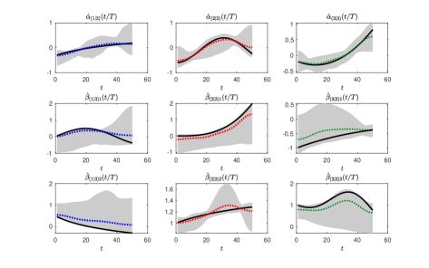
Figure 4: Estimates of the grouped frontiers for DGP3M with $N=500$ and $T=50$

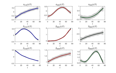
Figure 5: Estimates of the grouped frontiers for DGP3M with $N=500$ and $T=75$

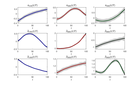
Figure 6: Estimates of the grouped frontiers for DGP3M with $N=500$ and $T=100$

Illustrated in Figures 4, 5 and 6 in Appendix D are the estimates of time-varying frontiers for $(N,T)=(500,50),(500,75),\text{and}(500,100)$. Black solid lines depict the true time-varying frontier, dotted lines show the mean of the estimated grouped frontiers averaged over 500 MC iterations, and the gray shaded region depicts the 90th percentile of the estimates. It is clear from Figure 4 that, while the mean over MC iterations is reasonably close to the true frontiers, the 90th percentile bands are wide, suggesting possible classification errors between neighboring groups. Figures 5 and 6 show that the accuracy of frontier grouping improves as $T$ increases. This is consistent with the theory developed, as the Step 2 classification using HAC is based on $\hat{\vartheta}_{i}=\left(\hat{\pi}_{i}^{\prime},\hat{\sigma}_{vi}\right)^{\prime}$ obtained using $T$ observations.

Results from other designs show similar patterns, which we omit for brevity.

Table 1: Performance of ICs for DGP3M

$(N,T)$	$K=1$	$K=2$	$K=3$	$K=4$	$\bar{\text{Pr}}(\bar{F})$	$\alpha^{0}-u$ uni	$\alpha^{0}-u$ mix
(100,50)	0.000	0.370	0.630	0.000	0.112	0.006	0.994
(100,75)	0.000	0.078	0.922	0.000	0.024	0.002	0.998
(100,100)	0.000	0.006	0.994	0.000	0.002	0.000	1.000
(250,50)	0.000	0.102	0.898	0.000	0.031	0.006	0.994
(250,75)	0.000	0.000	1.000	0.000	0.031	0.000	1.000
(250,100)	0.000	0.000	1.000	0.000	0.031	0.000	1.000
(500,50)	0.000	0.008	0.992	0.000	0.003	0.002	0.998
(500,75)	0.000	0.000	1.000	0.000	0.003	0.000	1.000
(500,100)	0.000	0.000	1.000	0.000	0.003	0.000	1.000
Note: Results for the baseline case $c_{\lambda}=\tilde{c}_{\lambda}=1$. Reported numbers are probabilities across replications.

Table 2: BIAS and RMSE over 500 MC iterations for DGP3M

		$\hat{\sigma}_{v(1)}$			$\hat{\sigma}_{v(2)}$			$\hat{\sigma}_{v(3)}$			$\hat{\tau}$			$\hat{\alpha}^{0}_{1}$			$\hat{\sigma}_{u1}$			$\hat{\alpha}^{0}_{2}$			$\hat{\sigma}_{u2}$
$(N,T)$		BIAS	RMSE		BIAS	RMSE		BIAS	RMSE		BIAS	RMSE		BIAS	RMSE		BIAS	RMSE		BIAS	RMSE		BIAS	RMSE
(100,50)		0.283	0.479		0.129	0.217		0.385	0.609		0.019	0.029		0.059	0.089		0.115	0.177		0.122	0.155		0.128	0.160
(100,75)		0.073	0.205		0.060	0.154		0.132	0.341		0.017	0.025		0.043	0.055		0.102	0.136		0.112	0.141		0.121	0.153
(100,100)		0.032	0.130		0.029	0.099		0.063	0.220		0.014	0.019		0.040	0.050		0.097	0.126		0.090	0.117		0.106	0.131
(250,50)		0.220	0.395		0.140	0.244		0.341	0.575		0.014	0.019		0.036	0.045		0.079	0.104		0.081	0.102		0.086	0.110
(250,75)		0.033	0.124		0.036	0.118		0.068	0.241		0.010	0.014		0.026	0.033		0.069	0.089		0.068	0.088		0.072	0.089
(250,100)		0.006	0.039		0.009	0.038		0.016	0.079		0.008	0.011		0.022	0.028		0.061	0.078		0.057	0.072		0.073	0.092
(500,50)		0.152	0.317		0.114	0.223		0.252	0.494		0.011	0.014		0.024	0.033		0.059	0.077		0.053	0.067		0.066	0.085
(500,75)		0.004	0.022		0.007	0.023		0.010	0.046		0.007	0.009		0.018	0.022		0.046	0.059		0.047	0.059		0.054	0.068
(500,100)		0.003	0.023		0.005	0.022		0.008	0.045		0.006	0.008		0.016	0.020		0.041	0.053		0.040	0.050		0.055	0.069

5 Application to the U.S. Commercial Banking Sector

In this section, we apply the developed method for stochastic production frontier model to analyze the cost efficiency of the U.S. large commercial banks in presence of a series of gradual deregulation that allowed banks to increase their capacity of operation. We use the same dataset used by Feng et al. (2017), and focus our analysis on a sample of banks that operate continuously over the period 1986 to 2005 (thereby mitigating the impact of entry and exit) with assets of at least $1 billion in 1986 dollars. As briefly explained in Feng et al. (2017), the banking sector over this period saw a number of gradual deregulation that allowed banks to increase the capacity of operation. In particular, the exact timing of the deregulation varied at the state level, and it was not until June 1997 that banks were allowed to operate across states as a result of the Riegle-Neal Interstate Banking and Branching Efficiency Act of 1994. Given this context, our method that allows us to group banks based on the time-varying frontiers is well suited to capture the effect of gradual deregulation, as well as to analyze the (in)efficiency of banks in presence of such deregulation.

To set the stage, let $i\in\{1,2,\cdots,N\}$ denote the banks, $t\in\{1,2,\cdots,T\}$ denote the time periods. The data is recorded in quarterly frequency, over 1986 to 2005, with $T=80$ and consists of $N=466$ banks. We assume that banks use three inputs to generate three outputs. Specifically, the inputs used are: (i) price of labor ($W_{it1}$), (ii) price of purchased funds ($W_{it2}$), and (iii) price of core deposits ($W_{it3}$). Generated outputs are: (i) consumer loans ($Y_{it1}$), (ii) non-consumer loans ($Y_{it2}$), consisting of industrial, commercial, and real estate loans, and (iii) securities ($Y_{it3}$), which includes all non-loan financial assets. Summary statistics of those variables are provided in Table 23 in Appendix D.

The particular variant of the PSF model we study is a panel stochastic cost frontier model adapted from Greene (2005b):

$$\log c_{it}^{*}=\alpha^{0}_{i} +\alpha_{i}(\tau_{t})+\beta_{i1}(\tau_{t})\log w_{it1}+\beta_{i2}(\tau_{t})\log w_{it2}$$

$$+\beta_{i3}(\tau_{t})\log y_{it1}+\beta_{i4}(\tau_{t})\log y_{it2}+\beta_{i5}(\tau_{t})\log y_{it3}+v_{it}+u_{i},$$ (5.1)

where linear homogeneity is imposed in input prices by the normalizations: $c_{it}^{*}=C_{it}/W_{it3}$, $w_{itl}=W_{itl}/W_{it3}$ for $l=1,2$ and $y_{itl}=Y_{itl}/W_{it3}$ for $l=1,2,3$. The inefficiency term $u_{i}\geq 0$ enters the model positively as cost frontier models are derived from the dual cost minimization problem of the firm where the cost function is assumed to be Cobb-Douglas. This specification of the model is rich enough to capture the production of banking services while keeping parsimony required for sieves regression.

5.1 Empirical Results

We estimate the model in (5) using the method described in the previous section, setting tuning parameters as in Section 4.2. We also check the sensitivity of parameter $c_{\lambda}$ in Step 3 and $\tilde{c}_{\lambda}$ in Step 5 of the proposed method as in Section 4.2. Different values of $c_{\lambda}$ and $\tilde{c}_{\lambda}$ deliver the same classification results.

As in the simulations, we set $\bar{K}=4$. The information criteria in step 3 selects the optimal number of group for the banks to be two, splitting $N=466$ banks into $(N_{1},N_{2})=(113,353)$. Figure 1 depict the scatter plots of the elements in $\hat{\vartheta}_{i}=(\hat{\pi}_{i}^{\prime},\hat{\sigma}_{vi})^{\prime}$, that collects the parameters obtained from individual level estimation in step 1 for classification in step 2. Note $m=\left\lfloor T^{1/5}\right\rfloor=2$, so $\hat{\vartheta}$ is a 12 by 1 vector. Individual estimates classified as group 1 are depicted as blue dots, while estimates classified as group 2 are depicted as red dots. Panel (a) depicts the scatter plot of the estimates $\hat{\pi}_{i1}$ against $\hat{\vartheta}_{i12}$, while panels (b)–(f) depict the respective coefficients on the inputs/outputs $\{w_{itl},y_{itl}\}$ against $\{w_{itl}B_{1}(\tau_{t}),y_{itl}B_{1}(\tau_{t})\}$. It is clear from Figure 1 that the classification is mostly driven by coefficient $\hat{\pi}_{i1}$ before $B_{1}(\tau_{t})$ and the coefficient $\hat{\pi}_{i8}$ before $y_{it2}$.

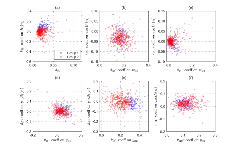
Figure 1: Scatter plot of elements in $\hat{\vartheta}_{i}=(\hat{\pi}_{i}^{\prime},\hat{\sigma}_{vi})^{\prime}$

• Note: Estimates classified as group 1 are plotted as blue dots, while that for group 2 are plotted as red dots.

Figure 2 depicts the frontiers. Top row depict the group 1 time-varying frontiers while the bottom row depict that of group 2. Solid lines in blue and red are the point estimates for group 1 and group 2 respectively, and the shaded regions depict the 95% confidence interval. It is evident that the there are substantial time-variations in the estimates, which may be a results of increasing the capacity of operation as a result of deregulation in the banking sector. Figure 3 shows the estimated economies of scale experienced by two groups of banks, $k\in\{1,2\}$ defined by the inverse of the sum of elasticities of output, $1/(\hat{\beta}_{(k)3}(\tau_{t})+\hat{\beta}_{(k)4}(\tau_{t})+\hat{\beta}_{(k)5}(\tau_{t}))-1$. The estimates on economies of scale are comparable to the ones found in Greene (2005b) and suggest some considerable time-variations for both groups, with group 2 banks enjoying larger economies of scale than group 1 banks.

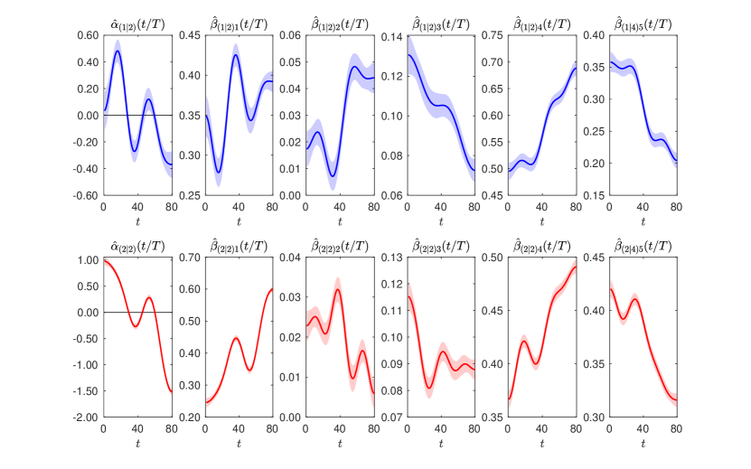
Figure 2: Grouped Frontiers of the U.S. Large Commercial Banks

• Note: Top row depict the group 1 time-varying frontiers while the bottom row depict that of group 2. Solid lines are the point estimates and the shaded regions are 95% confidence interval.

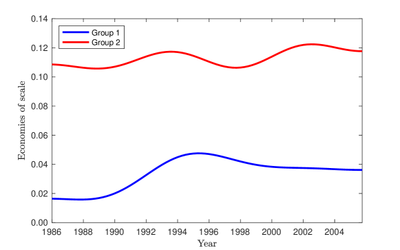
Figure 3: Estimates of Economy of Scale

• Note: Estimates of the economies of scale for each groups are calculated using the point estimates $\hat{\beta}_{(k)l}(\tau_{t})$ for $l=3,4,5$ and $k=1,2$.

Results from Step 5 suggests that intercept and idiosyncratic random effects terms, $\alpha^{0}-u$, possess a mixture structure. This result indicates that not only frontiers form two distinct groups, but so does the level terms that represent the efficiency of individual banks. The estimated values of the parameters along with standard errors are presented in Table 3. The results suggest that there are no substantial difference in the standard deviation of random noise, $\hat{\sigma}_{v}$s, though significant differences in the level term, $\hat{\alpha}^{0}$s, and the standard deviation of the inefficiency terms.

Table 3: Estimates of $\hat{\sigma}_{v}$s and $\hat{\varrho}$

$\hat{\sigma}_{v(1)}$	$\hat{\sigma}_{v(2)}$	$\hat{\tau}$	$\hat{\alpha}^{0}_{1}$	$\hat{\sigma}_{u1}$	$\hat{\alpha}^{0}_{2}$	$\hat{\sigma}_{u2}$
0.0862	0.0855	0.8748	0.0157	0.4426	0.6161	0.7756
(0.0041)	(0.0008)	(0.1017)	(0.3960)	(0.0362)	(0.1708)	(0.0235)

• Note: Reported in parentheses are the standard errors. We employ numerical differentiation to calculate the standard errors of $\hat{\varrho}$.

6 Conclusion

We have presented a panel stochastic frontier model that incorporates latent group structures. We detail the framework and customize the estimation procedure to align with its distinct features. Practical tuning parameters are recommended based on simulation findings. We apply the proposed method to analyze the cost efficiencies in the U.S. commercial banking sector and find evidence of group structures in both the frontier and efficiencies among large commercial banks.

Several extensions are worth mentioning. First, we have assumed the inefficiency term $u_{i}$ to be constant over time. It is possible to vary inefficiency term over time via deterministic function of time. Second, panel data literature that aims to recover latent group structures have allowed for structural breaks rather than smooth changes we have considered and group membership to vary (see, for example, Okui and Wang, 2021; Lumsdaine et al., 2023; Wang et al., 2024). We leave this for future research.

Appendix

Additional Notation. For the deterministic series $\{a_{n},b_{n}\}_{n=1}^{\infty}$, we denote $a_{n}\lesssim b_{n}$ if $\limsup_{n\rightarrow\infty}\left|a_{n}/b_{n}\right|\leq C$ for some constant $C$ that does not depend on $n$, $a_{n}\gtrsim b_{n}$ if $b_{n}\lesssim a_{n}$, $a_{n}\ll b_{n}$ if $a_{n}=o(b_{n})$, and $a_{n}\gg b_{n}$ if $b_{n}\ll a_{n}$. $\propto_{P}$ denotes proportional in probability, e.g., $x_{n}\propto_{P}y_{n}$ indicates that both $x_{n}=O_{P}(y_{n})$ and $y_{n}=O_{P}(x_{n})$ hold. $A^{c}$ denotes the complement of $A$. $C$ and $M$ denote some positive constants that may vary from line to line.

Appendix A The Approximation of the Likelihood Function

We derive the likelihood function incorporating approximations of $\alpha$ and $\beta$. Using the last line of (2.3),

$$y_{it} \approx\alpha^{0}_{i}-u_{i}+z_{it}^{\prime}\pi_{i}^{0}+v_{it}$$

$$=\alpha^{0}_{i}+z_{it}^{\prime}\pi_{i}^{0}+\varepsilon_{it}.$$ (A.1)

The primary distinction between the above approximation and (2.3) is that we do not separate $u_{i}$ from $\varepsilon_{it}$.

We first derive the likelihood function when the distribution of $\alpha^{0}_{i}-u_{i}$ is unique. We adopt the notation used in Yao et al. (2019) for the following presentation. Let

$$\sigma_{i}^{2}=\sigma_{vi}^{2}+T\sigma_{u}^{2},$$

$$\rho_{i}=\sigma_{u}/\sigma_{vi},$$

$$\mu_{i\ast}=-\frac{\sigma_{u}^{2}}{\sigma_{i}^{2}}\sum_{t=1}^{T}\varepsilon_{it},\quad\text{and}$$

$$\sigma_{i\ast}^{2}=\frac{\sigma_{u}^{2}\sigma_{vi}^{2}}{\sigma_{i}^{2}},$$

then

$$\sigma_{vi}^{2}=\frac{\sigma_{i}^{2}}{1+T\rho_{i}^{2}}.$$

We denote the density and cumulative distribution functions of a standard normal distribution as $\phi(\cdot)$ and $\Phi(\cdot)$, respectively. Following calculations similar to those in Yao et al. (2019), the density of $\varepsilon_{i}=\left(\varepsilon_{i1},\ldots,\varepsilon_{iT}\right)^{\prime}$ is given by

$$f\left(\varepsilon_{i};\sigma_{u}^{2},\sigma_{vi}^{2}\right) =\frac{2}{\sigma_{vi}^{T-1}\sigma_{i}}\left[1-\Phi\left(-\frac{\mu_{i\ast}}{\sigma_{i\ast}}\right)\right]\left[\prod_{t=1}^{T}\phi\left(\frac{\varepsilon_{it}}{\sigma_{vi}}\right)\right]\exp\left(\frac{1}{2}\left(-\frac{\mu_{i\ast}}{\sigma_{i\ast}}\right)^{2}\right),$$

which implies

$$\log f\left(\varepsilon_{i};\sigma_{u}^{2},\sigma_{vi}^{2}\right) =C-\frac{(T-1)}{2}\log\sigma_{vi}^{2}-\frac{1}{2}\log\left(\sigma_{vi}^{2}+T\sigma_{u}^{2}\right)$$

$$\quad+\log\left[1-\Phi\left(-\frac{\mu_{i\ast}}{\sigma_{i\ast}}\right)\right]+\frac{1}{2}\left(\frac{\mu_{i\ast}}{\sigma_{i\ast}}\right)^{2}-\frac{\sum_{t=1}^{T}\varepsilon_{it}^{2}}{2\sigma_{vi}^{2}},$$

for some constant $C$ that does not depend on the parameters to be estimated. Recall that $\vartheta_{i}=\left(\pi_{i}^{0\prime},\sigma_{vi}^{2}\right)^{\prime}$. Using the approximation in (A.1), the log-likelihood density function for $y_{i}=\left(y_{i1},\ldots,y_{iT}\right)^{\prime}$ is given by

$$\log f\left(y_{i}\mid x_{i};\alpha^{0}_{i},\sigma_{u}^{2},\vartheta_{i}\right) \approx C-\frac{(T-1)}{2}\log\sigma_{vi}^{2}-\frac{1}{2}\log\left(\sigma_{vi}^{2}+T\sigma_{u}^{2}\right)$$ (A.2)

$$\quad+\log\left[1-\Phi\left(-\frac{\tilde{\mu}_{\ast i}}{\sigma_{\ast i}}\right)\right]+\frac{1}{2}\left(\frac{\tilde{\mu}_{\ast i}}{\sigma_{\ast i}}\right)^{2}-\frac{\sum_{t=1}^{T}\tilde{\varepsilon}_{it}^{2}}{2\sigma_{vi}^{2}},$$

with

$$\tilde{\varepsilon}_{it} =y_{it}-\alpha^{0}_{i}-z_{it}^{\prime}\pi_{i}^{0},\text{ and}$$

$$\tilde{\mu}_{i\ast} =-\frac{\sigma_{u}^{2}}{\sigma_{i}^{2}}\sum_{t=1}^{T}\tilde{\varepsilon}_{it}.$$

We now consider the case when $\alpha^{0}_{i}-u_{i}$ is distributed as $\alpha^{0}_{1}-\left|N\left(0,\sigma_{u1}^{2}\right)\right|$ and $\alpha^{0}_{2}-\left|N\left(0,\sigma_{u2}^{2}\right)\right|$ with probabilities $\tau^{0}$ and $1-\tau^{0}$, respectively, for some $0<\tau^{0}<1$. This log-likelihood function is denoted as $\log\tilde{f}$ and can be derived as:

$$\log\tilde{f}\left(y_{i}\left|x_{i};\alpha^{0}_{1},\sigma_{u1}^{2},\alpha^{0}_{2},\sigma_{u2}^{2},\tau^{0},\vartheta_{i}\right.\right)$$ (A.3)

$$= \log\left[\tau^{0}f\left(y_{i}\left|x_{i};\alpha^{0}_{1},\sigma_{u1}^{2},\vartheta_{i}\right.\right)+\left(1-\tau^{0}\right)f\left(y_{i}\left|x_{i};\alpha^{0}_{2},\sigma_{u2}^{2},\vartheta_{i}\right.\right)\right],$$

where $f\left(y_{i}\mid x_{i};\alpha^{0}_{1},\sigma_{u1}^{2},\vartheta_{i}\right)$ and $f\left(y_{i}\mid x_{i};\alpha^{0}_{2},\sigma_{u2}^{2},\vartheta_{i}\right)$ are defined in (A.2).

Appendix B HAC Method

In this section of the appendix, we describe the Hierarchical Agglomerative Clustering (HAC) method used as part of the proposed method. We largely adopt the description from Chapter 4 of Everitt et al. (2011).

HAC is a bottom-up clustering approach that starts by treating each data point as an individual cluster. Clusters are then iteratively merged based on their similarity, resulting in a hierarchical structure of clusters. This process continues until a specified number of clusters is achieved or all data points are merged into a single cluster.

A commonly used approach within HAC is Ward’s method (Ward, 1963), which focuses on minimizing the variance within clusters. In each iteration, Ward’s method merges the two clusters that result in the smallest increase in the total within-cluster variance (also known as the “error sum of squares”). This criterion aims to form compact clusters with minimal internal variation.

The distance metric in Ward’s method is computed by evaluating the increase in variance that would result from merging two clusters, effectively prioritizing pairs of clusters with the smallest “distance.” Specifically, for clusters $A$ and $B$, the distance $d_{AB}$ in Ward’s method is defined as:

$$d_{AB}=\frac{|A||B|}{|A|+|B|}\|\bar{x}_{A}-\bar{x}_{B}\|^{2},$$

where $|A|$ and $|B|$ represent the sizes of clusters $A$ and $B$, and $\bar{x}_{A}$ and $\bar{x}_{B}$ denote their centroids. This distance metric reflects the increase in the sum of squares within clusters when clusters $A$ and $B$ are merged.

Appendix C Main Proofs

The main proofs in this section are built on technical lemmas in Appendix F. We first present some well known results that are useful for the proofs in this appendix.

We let $b_{il}$, $l=0,1,...,p$, denote the bias term from approximations. Specifically,

$$b_{i0}\left(s\right)=\alpha_{i}\left(s\right)-\mathbb{B}_{-0}^{m}\left(s\right)^{\prime}\pi_{i0}^{0}\text{ and $b_{il}\left(s\right)$$=\beta_{il}\left(s\right)-\mathbb{B}^{m}\left(s\right)^{\prime}\pi_{il}^{0}$},$$ (C.1)

for $s\in\left[0,1\right]$, and $\xi_{it}$ collects the bias term in $y_{it}$:

$$\xi_{it}\equiv{\displaystyle b_{i0}\left(\tau_{t}\right)+\sum_{l=1}^{p}}x_{itl}b_{il}\left(\tau_{t}\right).$$ (C.2)

With this notation and (2.3),

$$y_{it}=\tilde{z}_{it}^{\prime}\tilde{\pi}_{i}^{0}+\xi_{it}+v_{it}.$$ (C.3)

We know from Chen (2007) that

$$\sup_{s\in\left[0,1\right]}\left|b_{il}\left(s\right)\right|=O\left(m^{-\kappa}\right)$$

holds by Assumption 4. Since $p$ is finite, clearly,

$$\max_{l=0,...,p}\sup_{s\in\left[0,1\right]}\left|b_{il}\left(s\right)\right|=O\left(m^{-\kappa}\right),$$ (C.4)

for $i=1,...,N.$ Using similar logic on $\alpha_{k}^{*}\left(\tau_{t}\right)$ and the fact $K^{*}$is fixed, we can obtain

$$\max_{k=1,...,K^{*}}\max_{l=0,...,p}\sup_{s\in\left[0,1\right]}\left|b_{kl}^{*}\left(s\right)\right|=O\left(m^{-\kappa}\right),$$ (C.5)

where

$$b_{k0}^{*}\left(s\right)=\alpha_{k}^{*}\left(s\right)-\mathbb{B}_{-0}^{m}\left(s\right)^{\prime}\pi_{i0}^{*0}\text{ and $b_{kl}^{*}\left(s\right)=\beta_{il}\left(s\right)-\mathbb{B}^{m}\left(s\right)^{\prime}\pi_{il}^{*0}$}\text{ for }l=1,...,p.$$

Proof of Theorem 3.1.

(i) is a direct result of Lemma F.5. To see that,

$$\Pr\left(\max_{i=1,2,...,N}\left\|\hat{\vartheta}_{i}-\vartheta_{i}\right\|>\epsilon\right) \leq\Pr\left(\max_{i=1,2,...,N}\left\|\hat{\pi}_{i}-\pi_{i}^{0}\right\|>\frac{\epsilon}{2}\right)+\Pr\left(\max_{i=1,2,...,N}\left\|\hat{\sigma}_{vi}^{2}-\sigma_{vi}^{2}\right\|>\frac{\epsilon}{2}\right)$$

$$\leq\Pr\left(\max_{i=1,2,...,N}\left\|\widehat{\tilde{\pi}}_{i}-\tilde{\pi}_{i}^{0}\right\|>\frac{\epsilon}{2}\right)+\Pr\left(\max_{i=1,2,...,N}\left\|\hat{\sigma}_{vi}^{2}-\sigma_{vi}^{2}\right\|>\frac{\epsilon}{2}\right)$$

$$=o\left(1\right),$$

where the second line holds by the fact that $\hat{\pi}_{i}$ is a sub-vector of $\widehat{\tilde{\pi}}_{i}$, and the last line applies the results in Lemma F.5.

(ii) Denote

$$L_{ii^{\prime}} \equiv\sum_{l=0}^{p}\left\|\pi_{il}^{0}-\pi_{i^{\prime}l}^{0}\right\|+\left|\sigma_{vi}-\sigma_{vi^{\prime}}\right|,\text{ and}$$

$$\hat{L}_{ii^{\prime}} \equiv\sum_{l=0}^{p}\left\|\hat{\pi}_{il}-\hat{\pi}_{i^{\prime}l}\right\|+\left|\hat{\sigma}_{vi}-\hat{\sigma}_{vi^{\prime}}\right|,$$

and

$$L_{jk}^{*}\equiv\sum_{l=0}^{p}\left\|\pi_{jl}^{*0}-\pi_{kl}^{*0}\right\|+\left|\sigma_{v(j)}^{\ast}-\sigma_{v(k)}^{\ast}\right|.$$

for $i,i^{\prime}=1,...,n$ and $j,k=1,...,K^{*}$. We first claim that

$$\min_{1\leq j\neq k\leq K^{*}}L_{jk}^{*}\geq\frac{1}{2}\underline{C}^{*}$$ (C.6)

holds after some large $m.$ We will show this claim at the end.

To show the result in (ii), it is equivalent to show that

$$\Pr\left(\max_{1\leq k\leq K^{*}}\max_{i,i^{\prime}\in G_{k|K^{*}}}\hat{L}_{ii^{\prime}}<\min_{1\leq j\neq k\leq K^{*}}\min_{i\in G_{j|K^{*}},i^{\prime}\in G_{k|K^{*}}}\hat{L}_{ii^{\prime}}\right)=1-o\left(1\right).$$

When $i,i^{\prime}\in G_{k|K^{*}},$ $L_{ii^{\prime}}=0$. Thus, the uniform convergence in (i) implies that, for $\epsilon=\underline{C}^{*}/6,$

$$\Pr\left(\max_{1\leq k\leq K^{*}}\max_{i,i^{\prime}\in G_{k|K^{*}}}\hat{L}_{ii^{\prime}}<\underline{C}^{*}/6\right)=1-o\left(1\right).$$ (C.7)

Denote this event as

$$A=\left\{\max_{1\leq k\leq K^{*}}\max_{i,i^{\prime}\in G_{k|K^{*}}}\hat{L}_{ii^{\prime}}<\underline{C}^{*}/6\right\}.$$

Conditional on this event $A$, the claim in (C.6) after some large $m$, the result in (C.7), and the triangular inequality imply that

$$\min_{1\leq j\neq k\leq K^{*}}\min_{i\in G_{j|K^{*}},i^{\prime}\in G_{k|K^{*}}}\hat{L}_{ii^{\prime}}$$

$$\geq \min_{1\leq j\neq k\leq K^{*}}L_{jk}^{*}-2\max_{i=1,...,n}\left(\sum_{l=0}^{p}\left\|\hat{\pi}_{il}-\pi_{il}^{0}\right\|+\left|\hat{\sigma}_{vi}-\sigma_{vi}\right|\right)$$

$$\geq \frac{\underline{C}^{*}}{2}-2\cdot\frac{\underline{C}^{*}}{6}=\underline{C}^{*}/6$$

$$> \max_{1\leq k\leq K^{*}}\max_{i,i^{\prime}\in G_{k|K^{*}}}\hat{L}_{ii^{\prime}}.$$

Therefore, after some large $m,$

$$\Pr\left(\max_{1\leq k\leq K^{*}}\max_{i,i^{\prime}\in G_{k|K^{*}}}\hat{L}_{ii^{\prime}}<\min_{1\leq j\neq k\leq K^{*}}\min_{i\in G_{j|K^{*}},i^{\prime}\in G_{k|K^{*}}}\hat{L}_{ii^{\prime}}\right)$$

$$\geq \Pr\left(\left.\max_{1\leq k\leq K^{*}}\max_{i,i^{\prime}\in G_{k|K^{*}}}\hat{L}_{ii^{\prime}}<\min_{1\leq j\neq k\leq K^{*}}\min_{i\in G_{j|K^{*}},i^{\prime}\in G_{k|K^{*}}}\hat{L}_{ii^{\prime}}\right|A\right)\Pr\left(A\right)$$

$$= \Pr\left(A\right)=1-o\left(1\right),$$

as desired.

We now show the claim in (C.6). Notice that for any $\pi_{1},\pi_{2}\in\mathbb{R}^{m},$

$$\left\|\mathbb{B}^{m}\left(s\right)^{\prime}\pi_{1}-\mathbb{B}^{m}\left(s\right)^{\prime}\pi_{2}\right\| =\left[\int_{0}^{1}\left(\sum_{j=0}^{m-1}B_{j}\left(s\right)\pi_{1j}-\sum_{j=0}^{m-1}B_{j}\left(s\right)\pi_{2j}\right)^{2}ds\right]^{1/2}$$

$$=\left[\int_{0}^{1}\sum_{j=0}^{m-1}B_{j}\left(s\right)^{2}\left(\pi_{1j}-\pi_{2j}\right)^{2}ds\right]^{1/2}=\left[\sum_{j=0}^{m-1}\left(\pi_{1j}-\pi_{2j}\right)^{2}\right]^{1/2}$$

$$=\left\|\pi_{1}-\pi_{2}\right\|,$$ (C.8)

where the second line holds by $\int_{0}^{1}B_{j}\left(s\right)B_{j^{\prime}}\left(s\right)ds=0$ for $j\neq j^{\prime},$and the third line holds by $\int_{0}^{1}B_{j}\left(s\right)^{2}ds=1.$

Using (C.8),

$$L_{jk}^{*}= \left\|\pi_{j0}^{*0}-\pi_{k0}^{*0}\right\|+\sum_{l=1}^{p}\left\|\pi_{jl}^{*0}-\pi_{kl}^{*0}\right\|+\left|\sigma_{v(j)}^{\ast}-\sigma_{v(k)}^{\ast}\right|$$

$$= \left\|\mathbb{B}_{-0}^{m}\left(s\right)^{\prime}\pi_{j0}^{*0}-\mathbb{B}_{-0}^{m}\left(s\right)^{\prime}\pi_{k0}^{*0}\right\|+\sum_{l=1}^{p}\left\|\mathbb{B}^{m}\left(s\right)^{\prime}\pi_{jl}^{*0}-\mathbb{B}^{m}\left(s\right)^{\prime}\pi_{kl}^{*0}\right\|+\left|\sigma_{v(j)}^{\ast}-\sigma_{v(k)}^{\ast}\right|$$

$$= \left\|\alpha_{j}^{*}-b_{j0}^{*}\left(s\right)-\alpha_{k}^{*}+b_{k0}^{*}\left(s\right)\right\|+\sum_{l=1}^{p}\left\|\beta_{jl}^{\ast}\left(s\right)-b_{jl}^{*}\left(s\right)-\beta_{kl}^{\ast}\left(s\right)+b_{jk}^{*}\left(s\right)\right\|+\left|\sigma_{v(j)}^{\ast}-\sigma_{v(k)}^{\ast}\right|$$

$$\geq \left\|\alpha_{j}^{*}-\alpha_{k}^{*}\right\|-\left\|b_{j0}^{*}\left(s\right)-b_{k0}^{*}\left(s\right)\right\|+\sum_{l=1}^{p}\left[\left\|\beta_{jl}^{\ast}-\beta_{kl}^{\ast}\right\|-\left\|b_{jl}^{*}\left(s\right)-b_{jk}^{*}\left(s\right)\right\|\right]+\left|\sigma_{v(j)}^{\ast}-\sigma_{v(k)}^{\ast}\right|$$

$$\geq \underline{C}^{*}-O\left(m^{-\kappa}\right),$$

where the fourth line holds by triangular inequality, and the last line holds by Assumption 5, the result in (C.5), and the fact that $p$ is fixed. Using the result in (C.5) and the fact that $K^{*}$ is fixed, then after some large $m,$

$$\min_{1\leq j\neq k\leq K^{*}}L_{jk}^{*}=\min_{1\leq j\neq k\leq K^{*}}\sum_{l=0}^{p}\left\|\pi_{jl}^{*0}-\pi_{kl}^{*0}\right\|+\left|\sigma_{v(j)}^{\ast}-\sigma_{v(k)}^{\ast}\right|\geq\frac{1}{2}\underline{C}^{*},$$

as desired. ∎

Proof of Theorem 3.2.

(i) Denote the event of correct classification as

$$\mathcal{M}=\left\{\left(\hat{G}_{1|K^{*}},\hat{G}_{2|K^{*}},\ldots,\hat{G}_{K^{*}|K^{*}}\right)=\left(G_{1|K^{*}},G_{2|K^{*}},\ldots,G_{K^{*}|K^{*}}\right)\right\}.$$

We first show the results conditional on the event $\mathscr{\mathcal{M}}.$

For each $i\in G_{k|K^{*}}$

$$y_{it}=\alpha^{0}-u_{i}+\underline{z}_{it}^{\prime}\pi_{\left(k\right)}^{*0}+\xi_{it}+v_{it},$$

where similar to how $\pi_{i}^{0}$ is defined, $\pi_{\left(k\right)}^{*0}$ collects coefficients for the approximation of $\alpha_{\left(k\right)}^{*}\left(s\right)$ and $\beta_{\left(k\right)}^{*}\left(s\right)$. Thus

$$\ddot{y}_{it}=\ddot{\underline{z}}_{it}^{\prime}\pi_{\left(k\right)}^{*0}+\ddot{\xi}_{it}+\ddot{v}_{it}.$$ (C.9)

Using (C.9),

$$\hat{\pi}_{\left(k|K^{*}\right)}^{*0}-\pi_{\left(k\right)}^{*0} =\left(\sum_{i\in G_{k|K^{*}}}\sum_{t=1}^{T}\underline{\ddot{z}}_{it}\underline{\ddot{z}}_{it}^{\prime}\right)^{-1}\left(\sum_{i\in G_{k|K^{*}}}\sum_{t=1}^{T}\underline{\ddot{z}}_{it}\ddot{\xi}_{it}\right)$$

$$+\left(\sum_{i\in G_{k|K^{*}}}\sum_{t=1}^{T}\underline{\ddot{z}}_{it}\underline{\ddot{z}}_{it}^{\prime}\right)^{-1}\left(\sum_{i\in G_{k|K^{*}}}\sum_{t=1}^{T}\underline{\ddot{z}}_{it}\ddot{v}_{it}\right)$$

$$\equiv A_{k1}+A_{k2},$$ (C.10)

where $\ddot{\xi}_{it}$ is the de-meaned $\xi_{it}$ (defined in (C.2)) over $t$ for observation $i$, and $\ddot{v}_{it}$ is similarly defined. With the decomposition in (C.10),

$$\sqrt{N_{k}T/\underline{m}}\mathbb{S}_{(k)}^{-1/2}\left[\hat{\theta}_{\left(k|K^{*}\right)}\left(s\right)-\theta_{\left(k\right)}^{*}\left(s\right)\right]$$

$$=\sqrt{N_{k}T/\underline{m}}\mathbb{S}_{(k)}^{-1/2}\mathbb{M_{B}}\left(s\right)\left[\hat{\pi}_{\left(k|K^{*}\right)}^{*0}-\pi_{\left(k\right)}^{*0}\right]$$

$$=\sqrt{N_{k}T/\underline{m}}\mathbb{S}_{(k)}^{-1/2}\mathbb{M_{B}}\left(s\right)A_{k1}+\sqrt{N_{k}T/\underline{m}}\mathbb{S}_{(k)}^{-1/2}\mathbb{M_{B}}\left(s\right)A_{k2}$$

$$=o_{P}\left(1\right)+\sqrt{N_{k}T/\underline{m}}\mathbb{S}_{(k)}^{-1/2}\mathbb{M_{B}}\left(s\right)A_{k2}$$

$$\stackrel{{\scriptstyle d}}{{\rightarrow}}N\left(0,I_{p+1}\right),$$ (C.11)

where the fourth line uses the result in Lemma F.8 and $N_{k}T/\underline{m}^{1+2\kappa}\rightarrow 0$ imposed in Assumption 10, and the last line holds by evoking the Crámer-Wold device on the result in Lemma F.9.

To facilitate exposition, let $\omega_{NT}\equiv\sqrt{N_{k}T/\underline{m}}\left(\mathbb{S}_{(k)}^{-1/2}\right)^{\prime}\left[\hat{\theta}_{\left(k|K^{*}\right)}\left(s\right)-\theta_{\left(k\right)}^{*}\left(s\right)\right].$ According to the definition of convergence in distribution, (C.11) implies that for any $\epsilon>0$ and any $x\in R$, there exists a big $N_{1}$ such that for all $N>N_{1}$

$$\left|P\left(\left.\omega_{NT}\leq x\right|\mathcal{M}\right)-\Phi\left(x\right)\right|<\frac{\epsilon}{3},$$

where $\Phi\left(\cdot\right)$ denotes the cumulative distribution function of the standard normal.

We now show the general results without conditional on $\mathscr{\mathcal{M}}$. Theorem 3.1 implies that there exists a big $N_{2}$ such that for all $N>N_{2}$

$$P\left(\mathcal{M}\right)>1-\frac{\epsilon}{3}.$$

Thus, for all $N>\max\left(N_{1},N_{2}\right)$ and any $x\in R$,

$$\left|P\left(\omega_{NT}\leq x\right)-\Phi\left(x\right)\right| =\left|P\left(\left.\omega_{NT}\leq x\right|\mathcal{M}\right)P\left(\mathcal{M}\right)+P\left(\left.\omega_{NT}\leq x\right|\mathcal{M}^{c}\right)P\left(\mathcal{M}^{c}\right)-\Phi\left(x\right)\right|$$

$$\leq\left|\left[P\left(\left.\omega_{NT}\leq x\right|\mathcal{M}\right)-\Phi\left(x\right)\right]P\left(\mathcal{M}\right)\right|+\left[1-P\left(\mathcal{M}\right)\right]\Phi\left(x\right)$$

$$+P\left(\left.\omega_{NT}\leq x\right|\mathcal{M}^{c}\right)P\left(\mathcal{M}^{c}\right)$$

$$\leq\frac{\epsilon}{3}+\frac{\epsilon}{3}+\frac{\epsilon}{3}=\epsilon,$$

which is the desired result by the definition of convergence in distribution.

(ii) We first show the results conditional on the event $\mathscr{\mathcal{M}}.$ Using the representation in (C.9),

$$\hat{\sigma}_{v\left(k|K^{*}\right)}^{2}-\sigma_{v\left(k\right)}^{*2}$$

$$=\frac{1}{N_{k}\left(T-1\right)}\sum_{i\in G_{k|K^{*}}}\sum_{t=1}^{T}\left(\ddot{y}_{it}-\underline{\ddot{z}}_{it}^{\prime}\hat{\pi}_{\left(k\right)}\right)^{2}-\sigma_{v\left(k\right)}^{*2}$$

$$=\frac{1}{N_{k}\left(T-1\right)}\sum_{i\in G_{k|K^{*}}}\sum_{t=1}^{T}\left[\ddot{\underline{z}}_{it}^{\prime}\left(\pi_{\left(k\right)}^{*0}-\hat{\pi}_{\left(k\right)}\right)+\ddot{\xi}_{it}+\ddot{v}_{it}\right]^{2}-\sigma_{v\left(k\right)}^{*2}$$

$$=\frac{1}{N_{k}\left(T-1\right)}\sum_{i\in G_{k|K^{*}}}\sum_{t=1}^{T}\ddot{v}_{it}^{2}-\sigma_{v\left(k\right)}^{*2}+\frac{1}{N_{k}\left(T-1\right)}\sum_{i\in G_{k|K^{*}}}\sum_{t=1}^{T}\left[\ddot{\underline{z}}_{it}^{\prime}\left(\pi_{\left(k\right)}^{*0}-\hat{\pi}_{\left(k\right)}\right)\right]^{2}$$

$$+\frac{1}{N_{k}\left(T-1\right)}\sum_{i\in G_{k|K^{*}}}\sum_{t=1}^{T}\ddot{\xi}_{it}^{2}+\frac{2}{N_{k}\left(T-1\right)}\sum_{i\in G_{k|K^{*}}}\sum_{t=1}^{T}\ddot{\underline{z}}_{it}^{\prime}\left(\pi_{\left(k\right)}^{*0}-\hat{\pi}_{\left(k\right)}\right)\left(\ddot{\xi}_{it}+\ddot{v}_{it}\right)$$

$$+\frac{2}{N_{k}\left(T-1\right)}\sum_{i\in G_{k|K^{*}}}\sum_{t=1}^{T}\ddot{\xi}_{it}\ddot{v}_{it}$$

$$\equiv A_{k1}+A_{k2}+A_{k3}+A_{k4}+A_{k5}.$$

We show that $A_{k2},A_{k3},A_{k4},$ and $A_{k5}$ are asymptotically negligible by demonstrating the rates for $A_{k2},A_{k3},A_{k4},$ and $A_{k5}$. We then move to the asymptotic distribution of $A_{k1}$.

For $A_{k2}$,

$$A_{k2} =\frac{1}{N_{k}\left(T-1\right)}\sum_{i\in G_{k|K^{*}}}\sum_{t=1}^{T}\left[\ddot{\underline{z}}_{it}^{\prime}\left(\pi_{\left(k\right)}^{*0}-\hat{\pi}_{\left(k\right)}\right)\right]^{2}$$

$$=\left(\pi_{\left(k\right)}^{*0}-\hat{\pi}_{\left(k\right)}\right)^{\prime}\left(\frac{1}{N_{k}\left(T-1\right)}\sum_{i\in G_{k|K^{*}}}\sum_{t=1}^{T}\ddot{\underline{z}}_{it}\ddot{\underline{z}}_{it}^{\prime}\right)\left(\pi_{\left(k\right)}^{*0}-\hat{\pi}_{\left(k\right)}\right)$$

$$=O_{P}\left(\left\|\pi_{\left(k\right)}^{*0}-\hat{\pi}_{\left(k\right)}\right\|^{2}\right)=O_{P}\left(\frac{\underline{m}}{N_{k}T}\right),$$ (C.12)

where the last line holds by full rank condition implied by Lemmas F.6 and F.7, and the rate we show in (i).

For $A_{k3},$ by the definition of $\xi_{it}$in (C.2), the rate in (C.5), and Assumption 10 (ii), we can obtain

$$A_{k3}=\frac{1}{N_{k}\left(T-1\right)}\sum_{i\in G_{k|K^{*}}}\sum_{t=1}^{T}\ddot{\xi}_{it}^{2}=O_{P}\left(\underline{m}^{-2\kappa}\right)=o_{P}\left(\frac{\underline{m}}{N_{k}T}\right).$$ (C.13)

For $A_{k4},$

$$A_{k4} =\frac{2}{N_{k}\left(T-1\right)}\sum_{i\in G_{k|K^{*}}}\sum_{t=1}^{T}\ddot{\underline{z}}_{it}^{\prime}\left(\pi_{\left(k\right)}^{*0}-\hat{\pi}_{\left(k\right)}\right)\left(\ddot{\xi}_{it}+\ddot{v}_{it}\right)$$

$$=\left(\pi_{\left(k\right)}^{*0}-\hat{\pi}_{\left(k\right)}\right)^{\prime}\left[\frac{2}{N_{k}\left(T-1\right)}\sum_{i\in G_{k|K^{*}}}\sum_{t=1}^{T}\ddot{\underline{z}}_{it}\ddot{\xi}_{it}\right]+\left(\pi_{\left(k\right)}^{*0}-\hat{\pi}_{\left(k\right)}\right)^{\prime}\frac{2}{N_{k}\left(T-1\right)}\sum_{i\in G_{k|K^{*}}}\sum_{t=1}^{T}\ddot{\underline{z}}_{it}\ddot{v}_{it}$$

$$=O_{P}\left(\sqrt{\frac{\underline{m}}{N_{k}T}}\underline{m}^{-\kappa}\right)+O_{P}\left(\sqrt{\frac{\underline{m}}{N_{k}T}}\cdot\sqrt{\frac{1}{N_{k}T}}\right)=o_{P}\left(\frac{\underline{m}}{N_{k}T}\right),$$ (C.14)

where for the third line we apply the result in Lemma F.8, the mixing condition across $t$ in Assumption 1, and the independence across $i$ in Assumption 7

For $A_{k5},$ again by the mixing condition across $t$, independence across $i$, and the rate in (C.5), we have

$$\text{Var}\left(\frac{2}{N_{k}\left(T-1\right)}\sum_{i\in G_{k|K^{*}}}\sum_{t=1}^{T}\ddot{\xi}_{it}\ddot{v}_{it}\right)\propto\frac{\underline{m}^{-2\kappa}}{NT}.$$

Using the Markov inequality, the above implies that

$$A_{k5}=O_{P}\left(\frac{\underline{m}^{-\kappa}}{\sqrt{NT}}\right)=o_{P}\left(\frac{\underline{m}}{N_{k}T}\right).$$ (C.15)

We turn to the leading term $A_{k1}:$

$$A_{k1} =\frac{1}{N_{k}\left(T-1\right)}\sum_{i\in G_{k|K^{*}}}\sum_{t=1}^{T}\ddot{v}_{it}^{2}-\sigma_{v\left(k\right)}^{2}$$

$$=\frac{1}{N_{k}\left(T-1\right)}\sum_{i\in G_{k|K^{*}}}\sum_{t=1}^{T}\left(\ddot{v}_{it}^{2}-\sigma_{v\left(k\right)}^{2}\right)+\frac{1}{T-1}\sigma_{v\left(k\right)}^{2}$$

$$=\frac{T}{T-1}\left[\frac{1}{N_{k}T}\sum_{i\in G_{k|K^{*}}}\sum_{t=1}^{T}\left(\ddot{v}_{it}^{2}-\sigma_{v\left(k\right)}^{2}\right)\right]+\frac{1}{T-1}\sigma_{v\left(k\right)}^{2}$$

$$=\frac{T}{T-1}\left[\frac{1}{N_{k}T}\sum_{i\in G_{k|K^{*}}}\sum_{t=1}^{T}\left(v_{it}^{2}-\sigma_{v\left(k\right)}^{2}\right)\right]-\frac{T}{T-1}\frac{1}{N_{k}}\sum_{i\in G_{k|K^{*}}}\bar{v}_{i}^{2}+\frac{1}{T-1}\sigma_{v\left(k\right)}^{2}$$

$$=\frac{T}{T-1}\left[\frac{1}{N_{k}T}\sum_{i\in G_{k|K^{*}}}\sum_{t=1}^{T}\left(v_{it}^{2}-\sigma_{v\left(k\right)}^{2}\right)\right]-\frac{1}{T-1}\frac{1}{N_{k}}\sum_{i\in G_{k|K^{*}}}\left(T\bar{v}_{i}^{2}-\sigma_{v\left(k\right)}^{2}\right)$$

$$\equiv A_{k11}+A_{k12}.$$

By the i.i.d. assumption on $v_{it},$

$$\sqrt{N_{k}T}\cdot A_{k11}\stackrel{{\scriptstyle d}}{{\rightarrow}}N\left(0,\text{Var}\left(\left.v_{it}^{2}\right|i\in G_{k|K^{*}}\right)\right).$$

Note $E\left(T\bar{v}_{i}^{2}\right)=\sigma_{v\left(k\right)}^{2}$ and $E\left(T^{2}\bar{v}_{i}^{4}\right)=O\left(1\right).$ By the independence across $i$ and Markov’s inequality,

$$A_{k12}=O_{P}\left(\frac{1}{T\sqrt{N_{k}}}\right),$$

which implies that

$$\sqrt{N_{k}T}\cdot A_{k12}=o_{P}\left(1\right).$$

Put the asymptotic distribution of $A_{k11}$ and the rate of $A_{k12}$ together, we obtain

$$\sqrt{N_{k}T}\cdot A_{k1}\stackrel{{\scriptstyle d}}{{\rightarrow}}N\left(0,\text{Var}\left(\left.v_{it}^{2}\right|i\in G_{k|K^{*}}\right)\right).$$ (C.16)

Equations (C.12), (C.13), (C.14), (C.15), and (C.16) imply that conditional on $\mathcal{M},$

$$\sqrt{N_{k}T}\left(\hat{\sigma}_{v\left(k|K^{*}\right)}^{2}-\sigma_{v\left(k\right)}^{*2}\right)\stackrel{{\scriptstyle d}}{{\rightarrow}}N\left(0,\text{Var}\left(\left.v_{it}^{2}\right|i\in G_{k|K^{*}}\right)\right).$$

The above result holds unconditionally, using a similar argument as in the proof of (i).

(iii) We only need to show the result conditional on the event $\mathcal{M}$. After that, we can show the unconditional result using the same logic as in the proofs of (i) and (ii). In the following, we assume that the event $\mathcal{M}$ happens.

In Appendix E.2, we show that the information matrix $\mathbb{I}$ and

$$E\left[\left.\sum_{k=1}^{K^{*}}\frac{N_{k}}{N}\cdot\left(\frac{\partial}{\partial\varrho}\log\tilde{f}_{i\left(k\right)}\left(\varrho\right)\right)\left(\frac{\partial}{\partial\varrho}\log\tilde{f}_{i\left(k\right)}\left(\varrho\right)\right)^{\prime}\right|_{\varrho=\varrho^{0}}\right]$$

are well behaved; that is, all elements in these two matrices are finite constants, not degenerated to 0, and they are positive definite.

Further, in (i) and (ii), we have shown that $\hat{\theta}_{\left(k|K^{*}\right)}\left(s\right)$ and $\hat{\sigma}_{v\left(k|K^{*}\right)}^{2}$ converge to the trues at the rates of $\sqrt{\frac{NT}{\underline{m}}}$ and $\sqrt{NT}$, respectively. Thus, the estimation errors of $\hat{\theta}_{\left(k|K^{*}\right)}\left(s\right)$ and $\hat{\sigma}_{v\left(k|\hat{K}\right)}^{2}$ have no impact on the convergence rate of $\hat{\varrho}$ and its asymptotic distribution, because $\hat{\varrho}$ supposedly converges to $\varrho^{0}$ at the rate of $\sqrt{N}$, which is slower than those of $\hat{\theta}_{\left(k|K^{*}\right)}\left(s\right)$ and $\hat{\sigma}_{v\left(k|K^{*}\right)}^{2}$.

By the independence across $i$, some standard analysis for the asymptotics of the MLE, see, e.g., Section 5.4.3 in Bickel and Doksum (2015), and the Slutsky’s Theorem, the asymptotic variance of $\hat{\varrho}$ is $N^{-1}$$\mathbb{I}$, and, by the Lindeberg Central Limit Theorem,

$$\sqrt{N}\mathbb{I}^{-1/2}\left(\hat{\varrho}-\varrho\right)\overset{d}{\rightarrow}N\left(0,I_{5}\right).$$

∎

Proof of Proposition 3.3.

(i) This is a result direct from Lemmas F.10 and F.11.

(ii) This is a result from Lemma F.12. ∎

Appendix D Figures and Tables

• Note: Black solid line depict the true time-varying frontier, dotted lines depict the mean of the estimated grouped frontiers averaged over 500 MC iterations, and the grey shaded region depict the 90 percentile of the estimates. The gray area is wide, due to mis-classification errors.

• Note: Black solid line depict the true time-varying frontier, dotted lines depict the mean of the estimated grouped frontiers averaged over 500 MC iterations, and the gray shaded region depict the 90 percentile of the estimates.

• Note: Black solid line depict the true time-varying frontier, dotted lines depict the mean of the estimated grouped frontiers averaged over 500 MC iterations, and the gray shaded region depict the 90 percentile of the estimates.

Table 4: BIAS and RMSE over 500 MC iterations for DGP1U

		$\hat{\sigma}_{v(1)}$			$\hat{\sigma}_{v(2)}$			$\hat{\alpha}^{0}$			$\hat{\sigma}_{u}$
$(N,T)$		BIAS	RMSE		BIAS	RMSE		BIAS	RMSE		BIAS	RMSE
(100,50)		0.024	0.033		0.064	0.069		0.048	0.061		0.065	0.081
(100,75)		0.013	0.018		0.033	0.036		0.041	0.052		0.065	0.080
(100,100)		0.012	0.016		0.034	0.037		0.035	0.044		0.064	0.080
(250,50)		0.010	0.015		0.035	0.038		0.036	0.043		0.041	0.051
(250,75)		0.007	0.009		0.016	0.018		0.027	0.033		0.041	0.050
(250,100)		0.006	0.008		0.016	0.018		0.024	0.030		0.039	0.050
(500,50)		0.006	0.008		0.016	0.018		0.030	0.035		0.030	0.038
(500,75)		0.004	0.005		0.011	0.012		0.023	0.028		0.028	0.035
(500,100)		0.004	0.005		0.011	0.012		0.018	0.022		0.029	0.037

Table 5: BIAS and RMSE over 500 MC iterations for DGP1M

		$\hat{\sigma}_{v(1)}$			$\hat{\sigma}_{v(2)}$			$\hat{\tau}$			$\hat{\alpha}^{0}_{1}$			$\hat{\sigma}_{u1}$			$\hat{\alpha}^{0}_{2}$			$\hat{\sigma}_{u2}$
$(N,T)$		BIAS	RMSE		BIAS	RMSE		BIAS	RMSE		BIAS	RMSE		BIAS	RMSE		BIAS	RMSE		BIAS	RMSE
(100,50)		0.024	0.033		0.064	0.069		0.014	0.022		0.061	0.077		0.114	0.150		0.096	0.130		0.125	0.157
(100,75)		0.013	0.018		0.033	0.036		0.011	0.016		0.051	0.065		0.097	0.123		0.075	0.100		0.115	0.142
(100,100)		0.012	0.016		0.034	0.037		0.010	0.013		0.045	0.056		0.092	0.115		0.067	0.087		0.113	0.141
(250,50)		0.010	0.015		0.035	0.038		0.007	0.010		0.040	0.050		0.061	0.078		0.058	0.073		0.077	0.093
(250,75)		0.007	0.009		0.016	0.018		0.006	0.008		0.031	0.040		0.059	0.074		0.046	0.058		0.076	0.094
(250,100)		0.006	0.008		0.016	0.018		0.006	0.009		0.030	0.038		0.057	0.071		0.043	0.056		0.074	0.093
(500,50)		0.006	0.008		0.016	0.018		0.005	0.007		0.034	0.041		0.045	0.056		0.042	0.053		0.053	0.066
(500,75)		0.004	0.005		0.011	0.012		0.005	0.006		0.027	0.033		0.043	0.054		0.035	0.044		0.048	0.061
(500,100)		0.004	0.005		0.011	0.012		0.005	0.006		0.020	0.026		0.043	0.054		0.032	0.040		0.050	0.062

Table 6: BIAS and RMSE over 500 MC iterations for DGP2U

		$\hat{\sigma}_{v(1)}$			$\hat{\sigma}_{v(2)}$			$\hat{\alpha}^{0}$			$\hat{\sigma}_{u}$
$(N,T)$		BIAS	RMSE		BIAS	RMSE		BIAS	RMSE		BIAS	RMSE
(100,50)		0.008	0.010		0.018	0.022		0.039	0.049		0.064	0.081
(100,75)		0.005	0.006		0.013	0.017		0.037	0.048		0.062	0.078
(100,100)		0.004	0.005		0.012	0.015		0.028	0.036		0.063	0.079
(250,50)		0.004	0.005		0.011	0.014		0.025	0.031		0.041	0.051
(250,75)		0.003	0.004		0.009	0.011		0.021	0.026		0.040	0.050
(250,100)		0.003	0.003		0.008	0.009		0.020	0.025		0.039	0.049
(500,50)		0.003	0.004		0.008	0.009		0.016	0.020		0.030	0.038
(500,75)		0.002	0.002		0.006	0.008		0.015	0.019		0.029	0.036
(500,100)		0.002	0.002		0.005	0.007		0.014	0.017		0.029	0.037

Table 7: BIAS and RMSE over 500 MC iterations for DGP2M

		$\hat{\sigma}_{v(1)}$			$\hat{\sigma}_{v(2)}$			$\hat{\tau}$			$\hat{\alpha}^{0}_{1}$			$\hat{\sigma}_{u1}$			$\hat{\alpha}^{0}_{2}$			$\hat{\sigma}_{u2}$
$(N,T)$		BIAS	RMSE		BIAS	RMSE		BIAS	RMSE		BIAS	RMSE		BIAS	RMSE		BIAS	RMSE		BIAS	RMSE
(100,50)		0.008	0.010		0.018	0.022		0.021	0.032		0.038	0.049		0.114	0.154		0.139	0.180		0.138	0.171
(100,75)		0.005	0.006		0.013	0.017		0.016	0.024		0.036	0.045		0.098	0.132		0.109	0.140		0.123	0.153
(100,100)		0.004	0.005		0.012	0.015		0.012	0.017		0.029	0.036		0.087	0.113		0.093	0.121		0.121	0.150
(250,50)		0.004	0.005		0.011	0.014		0.014	0.018		0.025	0.030		0.068	0.088		0.085	0.108		0.086	0.105
(250,75)		0.003	0.004		0.009	0.011		0.011	0.014		0.020	0.025		0.065	0.085		0.073	0.091		0.084	0.102
(250,100)		0.003	0.003		0.008	0.009		0.010	0.013		0.020	0.025		0.061	0.078		0.068	0.086		0.082	0.100
(500,50)		0.003	0.004		0.008	0.009		0.014	0.016		0.017	0.021		0.056	0.072		0.065	0.079		0.064	0.079
(500,75)		0.002	0.002		0.006	0.008		0.011	0.013		0.015	0.019		0.055	0.070		0.054	0.068		0.052	0.067
(500,100)		0.002	0.002		0.005	0.007		0.008	0.010		0.014	0.017		0.049	0.063		0.049	0.061		0.055	0.069

Table 8: BIAS and RMSE over 500 MC iterations for DGP3U

		$\hat{\sigma}_{v(1)}$			$\hat{\sigma}_{v(2)}$			$\hat{\sigma}_{v(3)}$			$\hat{\alpha}^{0}$			$\hat{\sigma}_{u}$
$(N,T)$		BIAS	RMSE		BIAS	RMSE		BIAS	RMSE		BIAS	RMSE		BIAS	RMSE
(100,50)		0.283	0.479		0.129	0.217		0.385	0.609		0.059	0.078		0.075	0.096
(100,75)		0.073	0.205		0.060	0.154		0.132	0.341		0.045	0.060		0.062	0.078
(100,100)		0.032	0.130		0.029	0.099		0.063	0.220		0.037	0.049		0.065	0.080
(250,50)		0.220	0.395		0.140	0.244		0.341	0.575		0.038	0.051		0.051	0.066
(250,75)		0.033	0.124		0.036	0.118		0.068	0.241		0.025	0.032		0.042	0.052
(250,100)		0.006	0.039		0.009	0.038		0.016	0.079		0.022	0.027		0.041	0.051
(500,50)		0.152	0.317		0.114	0.223		0.252	0.494		0.027	0.037		0.041	0.053
(500,75)		0.004	0.022		0.007	0.023		0.010	0.046		0.018	0.023		0.029	0.037
(500,100)		0.003	0.023		0.005	0.022		0.008	0.045		0.016	0.021		0.027	0.034

Table 9: Performance of ICs for DGP1U

$(N,T)$	$K=1$	$K=2$	$K=3$	$K=4$	$\alpha^{0}-u$ unique	$\alpha^{0}-u$ mix
(100,50)	0.000	1.000	0.000	0.000	0.916	0.084
(100,75)	0.000	1.000	0.000	0.000	0.908	0.092
(100,100)	0.000	1.000	0.000	0.000	0.934	0.066
(250,50)	0.000	1.000	0.000	0.000	0.988	0.012
(250,75)	0.000	1.000	0.000	0.000	0.986	0.014
(250,100)	0.000	1.000	0.000	0.000	0.996	0.004
(500,50)	0.000	1.000	0.000	0.000	1.000	0.000
(500,75)	0.000	1.000	0.000	0.000	0.998	0.002
(500,100)	0.000	1.000	0.000	0.000	1.000	0.000
Note: Results for the baseline case $c_{\lambda}=\tilde{c}_{\lambda}=1$. Reported numbers are probabilities across replications.

Table 10: Performance of ICs for DGP1M

$(N,T)$	$K=1$	$K=2$	$K=3$	$K=4$	$\alpha^{0}-u$ unique	$\alpha^{0}-u$ mix
(100,50)	0.000	1.000	0.000	0.000	0.000	1.000
(100,75)	0.000	1.000	0.000	0.000	0.000	1.000
(100,100)	0.000	1.000	0.000	0.000	0.000	1.000
(250,50)	0.000	1.000	0.000	0.000	0.000	1.000
(250,75)	0.000	1.000	0.000	0.000	0.000	1.000
(250,100)	0.000	1.000	0.000	0.000	0.000	1.000
(500,50)	0.000	1.000	0.000	0.000	0.000	1.000
(500,75)	0.000	1.000	0.000	0.000	0.000	1.000
(500,100)	0.000	1.000	0.000	0.000	0.000	1.000
Note:Results for the baseline case $c_{\lambda}=\tilde{c}_{\lambda}=1$. Reported numbers are probabilities across replications.

Table 11: Performance of ICs for DGP2U

$(N,T)$	$K=1$	$K=2$	$K=3$	$K=4$	$\alpha^{0}-u$ unique	$\alpha^{0}-u$ mix
(100,50)	0.000	1.000	0.000	0.000	0.842	0.158
(100,75)	0.000	1.000	0.000	0.000	0.844	0.156
(100,100)	0.000	1.000	0.000	0.000	0.854	0.146
(250,50)	0.000	1.000	0.000	0.000	0.978	0.022
(250,75)	0.000	1.000	0.000	0.000	0.978	0.022
(250,100)	0.000	1.000	0.000	0.000	0.992	0.008
(500,50)	0.000	1.000	0.000	0.000	1.000	0.000
(500,75)	0.000	1.000	0.000	0.000	1.000	0.000
(500,100)	0.000	1.000	0.000	0.000	1.000	0.000
Note: Results for the baseline case $c_{\lambda}=\tilde{c}_{\lambda}=1$. Reported numbers are probabilities across replications.

Table 12: Performance of ICs for DGP2M

$(N,T)$	$K=1$	$K=2$	$K=3$	$K=4$	$\alpha^{0}-u$ unique	$\alpha^{0}-u$ mix
(100,50)	0.000	1.000	0.000	0.000	0.000	1.000
(100,75)	0.000	1.000	0.000	0.000	0.000	1.000
(100,100)	0.000	1.000	0.000	0.000	0.000	1.000
(250,50)	0.000	1.000	0.000	0.000	0.000	1.000
(250,75)	0.000	1.000	0.000	0.000	0.000	1.000
(250,100)	0.000	1.000	0.000	0.000	0.000	1.000
(500,50)	0.000	1.000	0.000	0.000	0.000	1.000
(500,75)	0.000	1.000	0.000	0.000	0.000	1.000
(500,100)	0.000	1.000	0.000	0.000	0.000	1.000
Note: Results for the baseline case $c_{\lambda}=\tilde{c}_{\lambda}=1$. Reported numbers are probabilities across replications.

Table 13: Performance of ICs for DGP3U

$(N,T)$	$K=1$	$K=2$	$K=3$	$K=4$	$\alpha^{0}-u$ unique	$\alpha^{0}-u$ mix
(100,50)	0.000	0.370	0.630	0.000	0.774	0.226
(100,75)	0.000	0.068	0.932	0.000	0.818	0.182
(100,100)	0.000	0.006	0.994	0.000	0.860	0.140
(250,50)	0.000	0.102	0.898	0.000	0.948	0.052
(250,75)	0.000	0.000	1.000	0.000	0.978	0.022
(250,100)	0.000	0.000	1.000	0.000	0.976	0.024
(500,50)	0.000	0.008	0.992	0.000	0.994	0.006
(500,75)	0.000	0.000	1.000	0.000	1.000	0.000
(500,100)	0.000	0.000	1.000	0.000	1.000	0.000
Note: Results for the baseline case $c_{\lambda}=\tilde{c}_{\lambda}=1$. Reported numbers are probabilities across replications.

Table 14: Sensitivity analysis for classification error in DGP1U and DGP1M

		$c_{\lambda}=3/2$			$c_{\lambda}=1$ (bench.)			$c_{\lambda}=3/4$
$(N,T)$			$\bar{\text{Pr}}(F)$			$\bar{\text{Pr}}(F)$			$\bar{\text{Pr}}(F)$
(100,50)			0.164			0.164			0.164
(100,75)			0.152			0.152			0.152
(100,100)			0.136			0.136			0.136
(250,50)			0.106			0.106			0.106
(250,75)			0.094			0.094			0.094
(250,100)			0.076			0.076			0.076
(500,50)			0.078			0.078			0.078
(500,75)			0.060			0.060			0.060
(500,100)			0.058			0.058			0.058

Table 15: Sensitivity analysis for classification error in DGP2U and DGP2M

		$c_{\lambda}=3/2$			$c_{\lambda}=1$ (bench.)			$c_{\lambda}=3/4$
$(N,T)$			$\bar{\text{Pr}}(F)$			$\bar{\text{Pr}}(F)$			$\bar{\text{Pr}}(F)$
(100,50)			0.000			0.000			0.000
(100,75)			0.000			0.000			0.000
(100,100)			0.000			0.000			0.000
(250,50)			0.000			0.000			0.000
(250,75)			0.000			0.000			0.000
(250,100)			0.000			0.000			0.000
(500,50)			0.000			0.000			0.000
(500,75)			0.000			0.000			0.000
(500,100)			0.000			0.000			0.000

Table 16: Sensitivity analysis for classification error in DGP3U and DGP3M

		$c_{\lambda}=3/2$			$c_{\lambda}=1$ (bench.)			$c_{\lambda}=3/4$
$(N,T)$			$\bar{\text{Pr}}(F)$			$\bar{\text{Pr}}(F)$			$\bar{\text{Pr}}(F)$
(100,50)			0.127			0.112			0.214
(100,75)			0.040			0.024			0.111
(100,100)			0.015			0.002			0.047
(250,50)			0.113			0.031			0.297
(250,75)			0.029			0.031			0.061
(250,100)			0.007			0.031			0.007
(500,50)			0.185			0.003			0.238
(500,75)			0.005			0.003			0.005
(500,100)			0.003			0.003			0.003

Table 17: Sensitivity analysis for $\alpha^{0}-u$ mixture structure for DGP1U

		$\tilde{c}_{\lambda}=3/2$			$\tilde{c}_{\lambda}=1$ (bench.)			$\tilde{c}_{\lambda}=3/4$
$(N,T)$		unique	mix		unique	mix		unique	mix
(100,50)		1.000	0.000		0.994	0.006		0.912	0.088
(100,75)		1.000	0.000		0.992	0.008		0.908	0.092
(100,100)		1.000	0.000		0.996	0.004		0.934	0.066
(250,50)		1.000	0.000		1.000	0.000		0.990	0.010
(250,75)		1.000	0.000		1.000	0.000		0.986	0.014
(250,100)		1.000	0.000		1.000	0.000		0.996	0.004
(500,50)		1.000	0.000		1.000	0.000		1.000	0.000
(500,75)		1.000	0.000		1.000	0.000		0.998	0.002
(500,100)		1.000	0.000		1.000	0.000		1.000	0.000

Table 18: Sensitivity analysis for $\alpha^{0}-u$ mixture structure for DGP1M

		$\tilde{c}_{\lambda}=3/2$			$\tilde{c}_{\lambda}=1$ (bench.)			$\tilde{c}_{\lambda}=3/4$
$(N,T)$		unique	mix		unique	mix		unique	mix
(100,50)		0.244	0.756		0.006	0.994		0.000	1.000
(100,75)		0.210	0.790		0.000	1.000		0.000	1.000
(100,100)		0.142	0.858		0.002	0.998		0.000	1.000
(250,50)		0.018	0.982		0.000	1.000		0.000	1.000
(250,75)		0.010	0.990		0.000	1.000		0.000	1.000
(250,100)		0.002	0.998		0.000	1.000		0.000	1.000
(500,50)		0.000	1.000		0.000	1.000		0.000	1.000
(500,75)		0.000	1.000		0.000	1.000		0.000	1.000
(500,100)		0.000	1.000		0.000	1.000		0.000	1.000

Table 19: Sensitivity analysis for $\alpha^{0}-u$ mixture structure for DGP2U

		$\tilde{c}_{\lambda}=3/2$			$\tilde{c}_{\lambda}=1$ (bench.)			$\tilde{c}_{\lambda}=3/4$
$(N,T)$		unique	mix		unique	mix		unique	mix
(100,50)		1.000	0.000		0.986	0.014		0.844	0.156
(100,75)		1.000	0.000		0.986	0.014		0.844	0.156
(100,100)		1.000	0.000		0.994	0.006		0.854	0.146
(250,50)		1.000	0.000		1.000	0.000		0.978	0.022
(250,75)		1.000	0.000		1.000	0.000		0.978	0.022
(250,100)		1.000	0.000		1.000	0.000		0.992	0.008
(500,50)		1.000	0.000		1.000	0.000		1.000	0.000
(500,75)		1.000	0.000		1.000	0.000		1.000	0.000
(500,100)		1.000	0.000		1.000	0.000		1.000	0.000

Table 20: Sensitivity analysis for $\alpha^{0}-u$ mixture structure for DGP2M

		$\tilde{c}_{\lambda}=3/2$			$\tilde{c}_{\lambda}=1$ (bench.)			$\tilde{c}_{\lambda}=3/4$
$(N,T)$		unique	mix		unique	mix		unique	mix
(100,50)		0.360	0.640		0.028	0.972		0.000	1.000
(100,75)		0.304	0.696		0.010	0.990		0.000	1.000
(100,100)		0.210	0.790		0.008	0.992		0.000	1.000
(250,50)		0.094	0.906		0.000	1.000		0.000	1.000
(250,75)		0.052	0.948		0.000	1.000		0.000	1.000
(250,100)		0.022	0.978		0.000	1.000		0.000	1.000
(500,50)		0.006	0.994		0.000	1.000		0.000	1.000
(500,75)		0.000	1.000		0.000	1.000		0.000	1.000
(500,100)		0.000	1.000		0.000	1.000		0.000	1.000

Table 21: Sensitivity analysis for $\alpha^{0}-u$ mixture structure for DGP3U

		$\tilde{c}_{\lambda}=3/2$			$\tilde{c}_{\lambda}=1$ (bench.)			$\tilde{c}_{\lambda}=3/4$
$(N,T)$		unique	mix		unique	mix		unique	mix
(100,50)		1.000	0.000		0.968	0.032		0.778	0.222
(100,75)		1.000	0.000		0.970	0.030		0.810	0.190
(100,100)		1.000	0.000		0.992	0.008		0.852	0.148
(250,50)		1.000	0.000		0.992	0.008		0.948	0.052
(250,75)		1.000	0.000		1.000	0.000		0.976	0.024
(250,100)		1.000	0.000		1.000	0.000		0.976	0.024
(500,50)		1.000	0.000		1.000	0.000		0.994	0.006
(500,75)		1.000	0.000		1.000	0.000		1.000	0.000
(500,100)		1.000	0.000		1.000	0.000		1.000	0.000

Table 22: Sensitivity analysis for $\alpha^{0}-u$ mixture structure for DGP3M

		$\tilde{c}_{\lambda}=3/2$			$\tilde{c}_{\lambda}=1$ (bench.)			$\tilde{c}_{\lambda}=3/4$
$(N,T)$		unique	mix		unique	mix		unique	mix
(100,50)		0.496	0.504		0.064	0.936		0.006	0.994
(100,75)		0.328	0.672		0.018	0.982		0.002	0.998
(100,100)		0.258	0.742		0.016	0.984		0.000	1.000
(250,50)		0.148	0.852		0.010	0.990		0.006	0.994
(250,75)		0.038	0.962		0.000	1.000		0.000	1.000
(250,100)		0.028	0.972		0.000	1.000		0.000	1.000
(500,50)		0.006	0.994		0.002	0.998		0.002	0.998
(500,75)		0.000	1.000		0.000	1.000		0.000	1.000
(500,100)		0.000	1.000		0.000	1.000		0.000	1.000

Table 23: Summary statistics of data used in the application

	MEAN	STD	MIN	MAX	$N\times T$
	Panel A: raw variables
$C_{it}$	$9.7974\times 10^{4}$	$7.0182\times 10^{5}$	$91.3791$	$2.2152\times 10^{7}$	$37280$
$W_{it1}$	$17.4185$	$9.7993$	$0.0913$	$252.9964$	$37280$
$W_{it2}$	$0.0073$	$0.0094$	$7.9946\times 10^{-7}$	$0.4393$	$37280$
$W_{it3}$	$0.02718$	$0.0200$	$6.1287\times 10^{-4}$	$0.4423$	$37280$
$Y_{it1}$	$2.1086\times 10^{5}$	$1.4001\times 10^{6}$	$4.2900$	$4.9625\times 10^{7}$	$37280$
$Y_{it2}$	$1.6894\times 10^{6}$	$1.0978\times 10^{7}$	$3020$	$3.1730\times 10^{8}$	$37280$
$Y_{it3}$	$1.3421\times 10^{6}$	$1.1142\times 10^{7}$	$2.4091\times 10^{3}$	$3.9273\times 10^{8}$	$37280$
	Panel B: variables used in regressions
$\log c_{it}^{*}$	12.8442	1.6370	9.1203	20.3854	37280
$\log w_{it1}$	6.5320	0.6060	2.8625	10.1837	37280
$\log w_{it2}$	-1.7023	1.0291	-8.4596	2.0101	37280
$\log y_{it1}$	9.8573	1.8283	1.4563	17.7200	37280
$\log y_{it2}$	11.8815	1.7312	8.0130	19.5754	37280
$\log y_{it3}$	11.6393	1.6402	7.7870	19.7886	37280

• Note: Raw variables in Panel A are denominated in Millions of 1986 USD. Variables in Panel B have been divided by $W_{it3}$ before taken logs.

Appendix E On $\mathbb{I}$ in Theorem 3.2

E.1 First and Second Order Derivatives

We use the notation in Appendix A. We assume $\alpha_{i}$, $\beta_{i}$, and $\sigma_{vi}^{2}$ are known because they are not the parameters of interest.

We first discuss the case when the distribution does not have a latent structure. The unknown parameters are $\left(\alpha^{0},\sigma_{u}^{2}\right)$ in this case. Note

$$\varepsilon_{it}=y_{it}-\alpha^{0}-\alpha\left(\tau_{t}\right)-x_{it}^{\prime}\beta\left(\tau_{t}\right)=v_{it}-u_{i},$$

$$f\left(\left.y_{i}\right|x_{i};\alpha^{0},\sigma_{u}^{2}\right) =\frac{2}{\sigma_{vi}^{T-1}\sqrt{\sigma_{vi}^{2}+T\sigma_{u}^{2}}}\left[1-\Phi\left(\frac{\sum_{t=1}^{T}\varepsilon_{it}}{\sigma_{vi}\sqrt{\sigma_{vi}^{2}/\sigma_{u}^{2}+T}}\right)\right]\left[\frac{1}{\left(2\pi\right)^{T/2}}\exp\left(-\frac{\sum_{t=1}^{T}\varepsilon_{it}^{2}}{2\sigma_{vi}^{2}}\right)\right]$$

$$\times\exp\left(\frac{1}{2}\frac{\left(\sum_{t=1}^{T}\varepsilon_{it}\right)^{2}}{\sigma_{vi}^{2}\left(\sigma_{vi}^{2}/\sigma_{u}^{2}+T\right)}\right),$$

and

$$\log f\left(\left.y_{i}\right|x_{i};\alpha^{0},\sigma_{u}^{2}\right)= C-\frac{(T-1)}{2}\log\sigma_{vi}^{2}-\frac{1}{2}\text{$\log$}\left(\sigma_{vi}^{2}+T\sigma_{u}^{2}\right)$$

$$+\log\left[1-\Phi\left(-\frac{\mu_{i\ast}}{\sigma_{i\ast}}\right)\right]+\frac{1}{2}\left(\frac{\mu_{i\ast}}{\sigma_{i\ast}}\right)^{2}-\frac{\sum_{t=1}^{T}\varepsilon_{it}^{2}}{2\sigma_{vi}^{2}},$$

with $\sigma_{i}^{2}=\sigma_{vi}^{2}+T\sigma_{u}^{2},$ $\rho_{i}=\sigma_{u}/\sigma_{vi},$ $\mu_{i\ast}=-\sigma_{u}^{2}\sum_{t=1}^{T}\varepsilon_{it}/\sigma_{i}^{2},$ $\sigma_{i\ast}^{2}=\sigma_{u}^{2}\sigma_{vi}^{2}/\sigma_{i}^{2}$, and a $C$ that does not depend on parameters.

By some straightforward calculations,

$$\frac{\partial}{\partial\sigma_{u}^{2}}\log f\left(\left.y_{i}\right|x_{i};\alpha^{0},\sigma_{u}^{2}\right) =-\frac{1}{2}\frac{T}{\sigma_{vi}^{2}+T\sigma_{u}^{2}}+\frac{\phi\left(-\frac{\mu_{i\ast}}{\sigma_{i\ast}}\right)}{1-\Phi\left(-\frac{\mu_{i\ast}}{\sigma_{i\ast}}\right)}\frac{-\sigma_{vi}}{2\sigma_{u}^{4}\left(\sigma_{vi}^{2}/\sigma_{u}^{2}+T\right)^{3/2}}\sum_{t=1}^{T}\varepsilon_{it}$$

$$+\frac{1}{2\sigma_{u}^{4}\left(\sigma_{vi}^{2}/\sigma_{u}^{2}+T\right)^{2}}\left(\sum_{t=1}^{T}\varepsilon_{it}\right)^{2},$$ (E.1)

$$\frac{\partial}{\partial\alpha^{0}}\log f\left(\left.y_{i}\right|x_{i};\alpha^{0},\sigma_{u}^{2}\right) =\frac{\phi\left(-\frac{\mu_{i\ast}}{\sigma_{i\ast}}\right)}{1-\Phi\left(-\frac{\mu_{i\ast}}{\sigma_{i\ast}}\right)}\frac{T}{\sigma_{vi}\sqrt{\sigma_{vi}^{2}/\sigma_{u}^{2}+T}}+\frac{1}{T^{-1}\sigma_{vi}^{2}+\sigma_{u}^{2}}\frac{1}{T}\left(\sum_{t=1}^{T}\varepsilon_{it}\right),$$ (E.2)

$$\frac{\partial^{2}}{\partial\sigma_{u}^{2}\partial\alpha^{0}}\log f\left(\left.y_{i}\right|x_{i};\alpha^{0},\sigma_{u}^{2}\right) =g\left(\frac{\mu_{i\ast}}{\sigma_{i\ast}}\right)\frac{-T}{2\sigma_{u}^{4}\left(\sigma_{vi}^{2}/\sigma_{u}^{2}+T\right)^{2}}\sum_{t=1}^{T}\varepsilon_{it}+\frac{\phi\left(-\frac{\mu_{i\ast}}{\sigma_{i\ast}}\right)}{1-\Phi\left(-\frac{\mu_{i\ast}}{\sigma_{i\ast}}\right)}\frac{T\sigma_{vi}}{2\sigma_{u}^{4}\left(\sigma_{vi}^{2}/\sigma_{u}^{2}+T\right)^{3/2}}$$

$$-\frac{T}{\sigma_{u}^{4}\left(\sigma_{vi}^{2}/\sigma_{u}^{2}+T\right)^{2}}\left(\sum_{t=1}^{T}\varepsilon_{it}\right),$$

$$\frac{\partial^{2}}{\partial(\alpha^{0})^{2}}\log f\left(\left.y_{i}\right|x_{i};\alpha^{0},\sigma_{u}^{2}\right) =g\left(\frac{\mu_{i\ast}}{\sigma_{i\ast}}\right)\frac{T^{2}}{\sigma_{vi}^{2}\left(\sigma_{vi}^{2}/\sigma_{u}^{2}+T\right)}-\frac{1}{T^{-1}\sigma_{vi}^{2}+\sigma_{u}^{2}},$$

and

$$\frac{\partial^{2}}{\partial\left(\sigma_{u}^{2}\right)^{2}}\log f\left(\left.y_{i}\right|x_{i};\alpha^{0},\sigma_{u}^{2}\right) =\frac{1}{2}\frac{T^{2}}{\left(\sigma_{vi}^{2}+T\sigma_{u}^{2}\right)^{2}}+g\left(\frac{\mu_{i\ast}}{\sigma_{i\ast}}\right)\frac{\sigma_{vi}^{2}}{4\sigma_{u}^{8}\left(\sigma_{vi}^{2}/\sigma_{u}^{2}+T\right)^{3}}\left(\sum_{t=1}^{T}\varepsilon_{it}\right)^{2}$$

$$+\frac{\phi\left(-\frac{\mu_{i\ast}}{\sigma_{i\ast}}\right)}{1-\Phi\left(-\frac{\mu_{i\ast}}{\sigma_{i\ast}}\right)}\frac{\left(\sigma_{vi}^{3}\sigma_{u}^{-4/3}+4T\sigma_{vi}\sigma_{u}^{2/3}\right)}{4\left(\sigma_{vi}^{2}\sigma_{u}^{2/3}+T\sigma_{u}^{8/3}\right)^{5/2}}\sum_{t=1}^{T}\varepsilon_{it}-\frac{T}{\left(\sigma_{vi}^{2}+T\sigma_{u}^{2}\right)^{3}}\left(\sum_{t=1}^{T}\varepsilon_{it}\right)^{2},$$

where

$$g\left(\frac{\mu_{i\ast}}{\sigma_{i\ast}}\right)=\left.\frac{d}{ds}\frac{\phi\left(-s\right)}{1-\Phi\left(-s\right)}\right|_{s=\frac{\mu_{i\ast}}{\sigma_{i\ast}}}=\left.\frac{-\phi\left(-s\right)-\phi^{\prime}\left(-s\right)\left[1-\phi\left(-s\right)\right]}{\left[1-\Phi\left(-s\right)\right]^{2}}\right|_{s=\frac{\mu_{i\ast}}{\sigma_{i\ast}}}.$$

In the case when the distribution possesses a latent structure, the log likelihood function becomes

$$\log\left[\tau f\left(y_{i}\left|x_{i};\alpha^{0}_{1},\sigma_{u1}^{2}\right.\right)+\left(1-\tau\right)f\left(\left.y_{i}\right|x_{i};\alpha^{0}_{2},\sigma_{u2}^{2}\right)\right]\equiv\log\left[\tau f_{1i}+\left(1-\tau\right)f_{2i}\right].$$

Then,

$$\frac{\partial}{\partial\tau}\log\left[\tau f_{1i}+\left(1-\tau\right)f_{2i}\right]=\frac{f_{1i}-f_{2i}}{\tau f_{1i}+\left(1-\tau\right)f_{2i}},\text{ and}$$

$$\frac{\partial^{2}}{\partial\tau^{2}}\log\left[\tau f_{1i}+\left(1-\tau\right)f_{2i}\right]=-\frac{\left(f_{1i}-f_{2i}\right)^{2}}{\left[\tau f_{1i}+\left(1-\tau\right)f_{2i}\right]^{2}}.$$

The derivatives with respect to other arguments $\alpha^{0}$ and $\sigma_{u}^{2}$ can be derived using the chain rule. For example,

$$\frac{\partial}{\partial\alpha^{0}_{1}}\log\left[\tau f_{1i}+\left(1-\tau\right)f_{2i}\right]=\frac{\tau\frac{\partial}{\partial\alpha^{0}_{1}}f_{1i}}{\tau f_{1i}+\left(1-\tau\right)f_{2i}}=\frac{\tau f_{1i}}{\tau f_{1i}+\left(1-\tau\right)f_{2i}}\cdot\frac{\partial}{\partial\alpha^{0}_{1}}\log f_{1i},\text{ and}$$

$$\frac{\partial}{\partial\sigma_{u1}^{2}}\log\left[\tau f_{1i}+\left(1-\tau\right)f_{2i}\right]=\frac{\tau\frac{\partial}{\partial\sigma_{u1}^{2}}f_{1i}}{\tau f_{1i}+\left(1-\tau\right)f_{2i}}=\frac{\tau f_{1i}}{\tau f_{1i}+\left(1-\tau\right)f_{2i}}\cdot\frac{\partial}{\partial\sigma_{u1}^{2}}\log f_{1i}.$$

E.2 Properties of $\mathbb{I}$

We verify that $\mathbb{I}$ behaves like a regular positive definite matrix in this section. The intuition of this result is as follows. Note $\tilde{f}_{i}\left(\varrho_{0}\right)$ is the density function for $\varepsilon_{it}=v_{it}-u_{i}$, and the parameters of interest are on the distribution of $u_{i}$ only. In other words, $v_{it}$ are nuisance for the estimation; observing $\varepsilon_{it}$ $T$ times does not provide more information than observing $u_{i}$ once for the estimation. Mathematically, one can see that the dominant components in $\frac{\partial}{\partial\varrho}\log\tilde{f}_{i}\left(\varrho\right)$ are functions of $u_{i}$ and do not grow as $T\rightarrow\infty$. Thus, the convergence rate of $\hat{\varrho}$ is $\sqrt{N}$ based on this intuition.

Without loss of generality, we assume that there is no group structure for the frontiers and $\sigma_{vi}^{2}$, that is, $K^{*}=1$. We show the result by assuming $\alpha^{0}=\alpha^{0}_{1}=\alpha^{0}_{2},$ and $\sigma_{u1}^{2}\neq\sigma_{u2}^{2}$. The case with $\alpha^{0}_{1}\neq\alpha^{0}_{2}$ can be similarly handled but with more tedious discussions. We show the result by using the following identity

$$\mathbb{I} =\left.-E\left[\frac{\partial^{2}}{\partial\varrho\partial\varrho^{\prime}}\log\tilde{f}_{i}\left(\varrho\right)\right]\right|_{\varrho=\varrho^{0}}$$

$$=\left.E\left[\frac{\partial}{\partial\varrho}\log\tilde{f}_{i}\left(\varrho\right)\cdot\frac{\partial}{\partial\varrho^{\prime}}\log\tilde{f}_{i}\left(\varrho\right)\right]\right|_{\varrho=\varrho^{0}}.$$ (E.3)

From the forms of $\frac{\partial}{\partial\sigma_{uj}^{2}}\log\left[\tau f_{1}+\left(1-\tau\right)f_{2}\right],$ $\frac{\partial}{\partial\alpha^{0}_{j}}\log\left[\tau f_{1}+\left(1-\tau\right)f_{2}\right],$ $j=1,2$, and

$$\frac{\partial}{\partial\tau}\log\left[\tau f_{1}+\left(1-\tau\right)f_{2}\right]$$

in Appendix E.1, they are clearly not linear dependent. If $T$ is fixed, $\mathbb{I}$ is just the information matrix for a regular likelihood function, and it is positive definite. Our analysis is complicated by the fact that $T\rightarrow\infty$. The diagonal of $\mathbb{I}$ might explode as $T\rightarrow\infty$. Thus, it suffices to show that the diagonals of $\mathbb{I}$ behave like regular positive constants, and we show that in the below.

The following is useful for the analysis. At the true values of parameters, $\varepsilon_{it}=v_{it}-u_{i}.$ So

$$T^{-1}\sum_{t=1}^{T}\varepsilon_{it} =-u_{i}+T^{-1}\sum_{t=1}^{T}v_{it}$$

$$=-u_{i}+O_{P}\left(T^{-1/2}\right).$$

Since $-u_{i}$ is negative, $T^{-1}\sum_{t=1}^{T}\varepsilon_{it}$ is negative with very high probability. Another implication is $\sum_{t=1}^{T}\varepsilon_{it}\propto_{P}-T+O_{P}\left(T^{1/2}\right).$ Using the definition of $\frac{\mu_{i\ast}}{\sigma_{i\ast}},$

$$\frac{\mu_{i\ast}}{\sigma_{i\ast}}=\frac{-1}{\sigma_{vi}\sqrt{\sigma_{vi}^{2}/\sigma_{u}^{2}+T}}\sum_{t=1}^{T}\varepsilon_{it}\propto_{P}\sqrt{T}+O_{P}\left(1\right).$$

The above implies $\Phi\left(-\frac{\mu_{i\ast}}{\sigma_{i\ast}}\right)=o_{P}\left(1\right),$

$$\frac{\phi\left(-\frac{\mu_{i\ast}}{\sigma_{i\ast}}\right)}{1-\Phi\left(-\frac{\mu_{i\ast}}{\sigma_{i\ast}}\right)}\propto_{P}\exp\left(-T\right),\frac{\phi\left(-\frac{\mu_{i\ast}}{\sigma_{i\ast}}\right)}{1-\Phi\left(-\frac{\mu_{i\ast}}{\sigma_{i\ast}}\right)}\sqrt{T}=o_{P}\left(1\right),$$

and

$$g\left(\frac{\mu_{i\ast}}{\sigma_{i\ast}}\right)\propto_{P}\exp\left(-T\right).$$

Applying the above for (E.2),

$$\frac{\partial}{\partial\alpha^{0}}\log f\left(\left.y_{i}\right|x_{i};\alpha^{0},\sigma_{u}^{2}\right)=-u_{i}+E\left(u_{i}\right)+o_{P}\left(1\right).$$

Similarly (E.1) implies

$$\frac{\partial}{\partial\sigma_{u}^{2}}\log f\left(\left.y_{i}\right|x_{i};\alpha^{0},\sigma_{u}^{2}\right)=\frac{u_{i}^{2}}{2\sigma_{u}^{4}}-\frac{1}{2\sigma_{u}^{2}}+o_{P}\left(1\right).$$

Some tedious yet straightforward calculations can yield

$$f\left(y_{i}\left|x_{i};\alpha^{0},\sigma_{u1}^{2}\right.\right)\propto_{P}f\left(\left.y_{i}\right|x_{i};\alpha^{0},\sigma_{u2}^{2}\right),$$

and

$$\frac{\partial}{\partial\tau}\log\left[\tau f_{1i}+\left(1-\tau\right)f_{2i}\right] =\frac{f_{1i}-f_{2i}}{\tau f_{1i}+\left(1-\tau\right)f_{2i}}.$$

$$=\frac{1-\sqrt{\left.\sigma_{u1}^{2}\right/\sigma_{u2}^{2}}\exp\left(\frac{1}{2}\left(\frac{1}{\sigma_{u1}^{2}}-\frac{1}{\sigma_{u2}^{2}}\right)u_{i}^{2}\right)}{\tau+\left(1-\tau\right)\sqrt{\left.\sigma_{u1}^{2}\right/\sigma_{2u}^{2}}\exp\left(\frac{1}{2}\left(\frac{1}{\sigma_{u1}^{2}}-\frac{1}{\sigma_{u2}^{2}}\right)u_{i}^{2}\right)}\left(1+o_{P}\left(1\right)\right).$$

The variance of the leading terms in $\frac{\partial}{\partial\alpha^{0}}\log f$, $\frac{\partial}{\partial\sigma_{u}^{2}}\log f,$ and $\frac{\partial}{\partial\tau}\log\left[\tau f_{1i}+\left(1-\tau\right)f_{2i}\right]$ are functions of $u_{i}$, and they are bounded and bounded away from zero.

Finally, since $f_{1i}\propto_{P}f_{2i},$ $\frac{\partial}{\partial\alpha^{0}_{j}}\log\left[\tau f_{1i}+\left(1-\tau\right)f_{2i}\right],$ $j=1,2,$ enjoys similar properties as $\frac{\partial}{\partial\alpha^{0}}\log f$. This is also the case for $\frac{\partial}{\partial\sigma_{uj}^{2}}\log\left[\tau f_{1i}+\left(1-\tau\right)f_{2i}\right],$$j=1,2.$

From the form of the derivatives, clearly, $\frac{\partial}{\partial\varrho_{j}}\log\left[\tau f_{1i}+\left(1-\tau\right)f_{2i}\right]$, $j=1,2,...,5,$ are not linearly dependent. Together with the fact that the variance of them are bounded and bounded away from zero, then for any $5\times 1$ vector $a,$

$$a^{\prime}\left.E\left[\frac{\partial}{\partial\varrho}\log\tilde{f}_{i}\left(\varrho\right)\cdot\frac{\partial}{\partial\varrho^{\prime}}\log\tilde{f}_{i}\left(\varrho\right)\right]\right|_{\varrho=\varrho^{0}}a\propto\left\|a\right\|^{2}.$$

This implies that $\mathbb{I}$ must be positive definite with bounded eigenvalues, using the identity in (E.3).

Appendix F Technical Lemmas

We collect technical lemmas and their proofs in this section. For an easier reference, we present the bodies of those lemmas first, followed by proofs.

Remark F.1 (Some inequalities).

We may apply the following inequalities in the proofs directly without referring them back to here. First

$$\Pr\left(X_{1}+X_{2}\geq C\right)\leq\Pr\left(X_{1}\geq\pi C\right)+\Pr\left(X_{2}\geq\left(1-\pi\right)C\right)$$

for any constant $\pi.$ That is because $\left\{X_{1}+X_{2}\geq C\right\}\subseteq\left\{X_{1}\geq\pi C\right\}\cup\left\{X_{1}\geq\left(1-\pi\right)C\right\}.$ Similarly, we have

$$\Pr\left(\sum_{i=1}^{n}X_{i}\geq C\right)\leq\sum_{i=1}^{n}\Pr\left(X_{i}\geq Cn^{-1}\right)\ \text{\emph{and} }\Pr\left(\max_{1\leq i\leq n}X_{i}\geq C\right)\leq\sum_{i=1}^{n}\Pr\left(X_{i}\geq C\right).$$

For any positive random variables $X_{1}$ and $X_{2}$ and positive constants $C_{1}$ and $C_{2},$

$$\Pr\left(X_{1}\cdot X_{2}\geq C_{1}\right)\leq\Pr\left(X_{1}\geq C_{1}/C_{2}\right)+\Pr\left(X_{2}\geq C_{2}\right),$$

due to the fact that $\left\{X_{1}\cdot X_{2}\geq C_{1}\right\}\subseteq\left\{X_{1}\geq C_{1}/C_{2}\right\}\cup\left\{X_{2}\geq C_{2}\right\}.$

Lemma F.1.

Suppose $e_{it}$ satisfies the mixing condition across $t$ in Assumption 1 (ii) and is identically distributed across $i$. In addition $\max_{t}E\left(\left|e_{it}\right|^{C_{q}}\right)<\infty,C_{q}>2,$ $T=N^{C}$ for some $C>0$, $m\rightarrow\infty$ as $N\rightarrow\infty$, then

(i) for any $\epsilon>0$ and any positive $1\leq\upsilon_{NT}\ll T^{1/2}\left(\log N\right)^{-2}$

$$\Pr\left(\max_{i=1,...,N}\left|\frac{1}{T}\sum_{t=1}^{T}\left[e_{it}-E\left(e_{it}\right)\right]\right|>\frac{\epsilon}{\upsilon_{NT}}\right)\lesssim\frac{NT\upsilon_{NT}^{C_{q}}\left(\log N\right)^{4C_{q}}}{T^{C_{q}}};$$

(ii) there exists a positive $M,$ such that

$$\Pr\left(\max_{i=1,...,N}\max_{l=0,1,...,p}\left|\frac{1}{T}\sum_{t=1}^{T}e_{it}b_{il}\left(\tau_{t}\right)\right|>Mm^{-\kappa}\right)\lesssim\frac{NT\left(\log N\right)^{4C_{q}}}{T^{C_{q}}},$$

where $b_{il}\left(\tau_{t}\right)$ is defined in (C.1).

Lemma F.2.

Suppose that Assumption 3 holds and $m/T\rightarrow 0$. For any $\tilde{\pi}\in\mathbb{R}^{m\left(p+1\right)},$

$$\frac{\underline{C}_{xx}}{2}\left\|\tilde{\pi}\right\|\leq\min_{1\leq i\leq N}\frac{1}{T}\sum_{t=1}^{T}E\left(\tilde{\pi}^{\prime}\tilde{z}_{it}\tilde{z}_{it}^{\prime}\tilde{\pi}\right)\leq\max_{1\leq i\leq N}\frac{1}{T}\sum_{t=1}^{T}E\left(\pi^{\prime}\tilde{z}_{it}\tilde{z}_{it}^{\prime}\pi\right)\leq 2\bar{C}_{xx}\left\|\tilde{\pi}\right\|,$$

after some large $T$.

Lemma F.3.

Suppose that Assumptions 1, 2, 3 and 6 (i) hold. Then

(i) for any $\epsilon>0,$

$$\Pr\left(\max_{1\leq i\leq N}\sup_{\tilde{\pi}\in\mathbb{R}^{m\left(p+1\right)},\left\|\tilde{\pi}\right\|=1}\left|\frac{1}{T}\sum_{t=1}^{T}\tilde{\pi}^{\prime}\tilde{z}_{it}\tilde{z}_{it}^{\prime}\tilde{\pi}-\frac{1}{T}\sum_{t=1}^{T}E\left(\tilde{\pi}^{\prime}\tilde{z}_{it}\tilde{z}_{it}^{\prime}\tilde{\pi}\right)\right|>\epsilon\right)\apprle\frac{Nm^{q/2+2}\left(\log N\right)^{2q}}{T^{q/2-1}};$$

(ii) there exist some positive and finite $\underline{C}_{zz}$ and $\bar{C}_{zz}$ such that

$$\Pr\left(\underline{C}_{zz}\leq\min_{1\leq i\leq N}\mu_{\min}\left(\frac{1}{T}\sum_{t=1}^{T}\tilde{z}_{it}\tilde{z}_{it}^{\prime}\right)\leq\max_{1\leq i\leq N}\mu_{\max}\left(\frac{1}{T}\sum_{t=1}^{T}\tilde{z}_{it}\tilde{z}_{it}^{\prime}\right)\leq\bar{C}_{zz}\right)$$

$$= 1-o\left(\frac{Nm^{q/2+2}\left(\log N\right)^{2q}}{T^{q/2-1}}\right)\text{.}$$

Lemma F.4.

Suppose Assumptions 1, 2, 4 and 6 (i) hold. Then

(i) for any $\epsilon>0,$

$$\Pr\left(\max_{i=1,...,N}\left\|\frac{1}{T}\sum_{t=1}^{T}\tilde{z}_{it}v_{it}\right\|>\epsilon\right)\lesssim\frac{Nm^{q/4}\left(\log N\right)^{2q}}{T^{q/2-1}};$$

(ii) for the $\xi_{it}$ defined in (C.2),

$$\Pr\left(\max_{i=1,...,N}\left\|\frac{1}{T}\sum_{t=1}^{T}\tilde{z}_{it}\xi_{it}\right\|>\epsilon\right)\lesssim\frac{Nm\left(\log N\right)^{2q}}{T^{q/2-1}}.$$

Lemma F.5.

Suppose that Assumptions 1, 2, 3, 4, and 6 hold. Then,

(i) for any small positive $\epsilon,$

$$\Pr\left(\max_{1\leq i\leq N}\left\|\widehat{\tilde{\pi}}_{i}-\tilde{\pi}_{i}^{0}\right\|>\epsilon\right)=o\left(1\right);$$

(ii) for any small positive $\epsilon,$

$$\Pr\left(\max_{1\leq i\leq N}\left\|\hat{\sigma}_{vi}^{2}-\sigma_{vi}^{2}\right\|>\epsilon\right)=o\left(1\right).$$

Lemma F.6.

Suppose Assumption 3 holds and $\underline{m}/T\rightarrow 0$. Then after some large $T,$

$$\frac{\underline{C}_{xx}}{2}\leq\min_{1\leq i\leq N}\mu_{\min}\left\{E\left(\frac{1}{T}\sum_{t=1}^{T}\underline{\ddot{z}}_{it}\underline{\ddot{z}}_{it}^{\prime}\right)\right\}\leq\max_{1\leq i\leq N}\mu_{\max}\left\{E\left(\frac{1}{T}\sum_{t=1}^{T}\underline{\ddot{z}}_{it}\underline{\ddot{z}}_{it}^{\prime}\right)\right\}\leq 2\bar{C}_{xx},$$

where $\underline{C}_{xx}$ and $\bar{C}_{xx}$ are defined in Lemma F.2.

Lemma F.7.

Suppose that Assumptions 1, 2, 3, 7 and 8 hold. Then for a fixed $k,$ $k=1,2,...,K^{*},$ and any $\epsilon>0,$

$$\Pr\left(\sup_{\pi\in\mathbb{R}^{\underline{m}-1+\underline{m}p},\left\|\pi\right\|=1}\left|\frac{1}{N_{k}}\sum_{i\in G_{k|K^{*}}}\left[\frac{1}{T}\sum_{t=1}^{T}\pi^{\prime}\underline{\ddot{z}}_{it}\underline{\ddot{z}}_{it}^{\prime}\pi-\frac{1}{T}\sum_{t=1}^{T}E\left(\pi^{\prime}\underline{\ddot{z}}_{it}\underline{\ddot{z}}_{it}^{\prime}\pi\right)\right]\right|>\epsilon\right)\apprle\frac{\underline{m}^{q/2+2}\left(\log N\right)^{2q}}{\left(NT\right)^{q/2-1}};$$

Lemma F.8.

Suppose Assumptions 1, 2, 3, 4, 6, 7, 8, and 10 hold. Then, the term

$$A_{k1}=\left(\sum_{i\in G_{k|K}}\sum_{t=1}^{T}\underline{\ddot{z}}_{it}\underline{\ddot{z}}_{it}^{\prime}\right)^{-1}\left(\sum_{i\in G_{k|K}}\sum_{t=1}^{T}\underline{\ddot{z}}_{it}\ddot{\xi}_{it}\right)$$

satisfies $\left\|A_{k1}\right\|=O_{P}\left(\underline{m}^{-\kappa}\right).$

Lemma F.9.

Suppose Assumptions 1, 2, 3, 4, 6, 7, 8, 9 , and 10 hold. For

$$A_{k2}=\left(\sum_{i\in G_{k|K}}\sum_{t=1}^{T}\underline{\ddot{z}}_{it}\underline{\ddot{z}}_{it}^{\prime}\right)^{-1}\left(\sum_{i\in G_{k|K}}\sum_{t=1}^{T}\underline{\ddot{z}}_{it}\ddot{v}_{it}\right)$$

and any $\left(p+1\right)\times 1$ vector $a$, it satisfies

$$\left.\sqrt{\frac{N_{k}T}{\underline{m}}}a^{\prime}\mathbb{M_{B}}\left(s\right)A_{k2}\right/\left\{a^{\prime}\left[\frac{\sigma_{v\left(k\right)}^{2}}{\underline{m}}\mathbb{M_{B}}\left(s\right)Q_{(k),zz}^{-1}\mathbb{M_{B}}\left(s\right)^{\prime}\right]a\right\}^{1/2}\stackrel{{\scriptstyle d}}{{\rightarrow}}N\left(0,1\right).$$

Lemma F.10.

Suppose Assumptions 1 - 8 hold. In addition, $\frac{\lambda_{NT}}{\sqrt{NT}}\rightarrow\infty$ and $\frac{\lambda_{NT}}{NT}\rightarrow 0$.

$$\Pr\left(\text{IC}\left(K^{*},\lambda_{NT}\right)<\text{IC}\left(K,\lambda_{NT}\right),1\leq K\leq K^{*}-1\right)\rightarrow 1.$$

Lemma F.11.

Suppose Assumptions 1 - 8 hold. In addition, $\frac{\lambda_{NT}}{\sqrt{NT}}\rightarrow\infty$ and $\frac{\lambda_{NT}}{NT}\rightarrow 0$.

$$\Pr\left(\text{IC}\left(K^{*},\lambda_{NT}\right)<\text{IC}\left(K,\lambda_{NT}\right),K^{*}+1\leq K\leq\bar{K}\right)\rightarrow 1.$$

Lemma F.12.

Suppose Assumptions 1 - 10 hold. $\tilde{\lambda}_{NT}$ satisfies $\tilde{\lambda}_{NT}\rightarrow\infty$ and $\frac{\tilde{\lambda}_{NT}}{N}\rightarrow 0$.

(i) If $\alpha^{0}-u_{i}$ comes from a unique distribution,

$$\Pr\left(\widetilde{\mathrm{IC}}_{1}\left(\tilde{\lambda}_{NT}\right)<\widetilde{\mathrm{IC}}_{2}\left(\tilde{\lambda}_{NT}\right)\right)\rightarrow 1.$$

(ii) If $\alpha^{0}-u_{i}$ comes from a mixture distribution as in Section 2.4,

$$\Pr\left(\widetilde{\mathrm{IC}}_{2}\left(\tilde{\lambda}_{NT}\right)<\widetilde{\mathrm{IC}}_{1}\left(\tilde{\lambda}_{NT}\right)\right)\rightarrow 1.$$

Proof of Lemma F.1.

(i) Set $C_{NT}=\upsilon_{NT}^{-1}T\left(\log N\right)^{-4}$. Define $\mathbf{1}_{it}=\mathbf{1}(\left|e_{it}\right|<C_{NT})$ and $\mathbf{\bar{1}}_{it}=1-\mathbf{1}_{it}$. With it, further define $e_{it}^{\left(1\right)}=e_{it}\mathbf{1}_{it}-E\left(e_{it}\mathbf{1}_{it}\right)$, $e_{it}^{\left(2\right)}=e_{it}\mathbf{\mathbf{\bar{1}}}_{it}$, and $e_{it}^{\left(3\right)}=E\left(e_{it}\mathbf{\mathbf{\bar{1}}}_{it}\right)$. Then

$$e_{it}-E\left(e_{it}\right)=e_{it}^{\left(1\right)}+e_{it}^{\left(2\right)}+e_{it}^{\left(3\right)}.$$

Let $v_{0}=\max_{t}\text{Var}\left(e_{it}\right)+2\sum_{s=t+1}^{T}\text{Cov}\left(e_{it},e_{is}\right)$, which is finite by the mixing condition in Assumption 1.

Using Bernstein inequality for strong mixing processes (e.g., Theorem 2 in Merlevede et al. (2009)), there exists positive constants $C_{1}$ and $C_{2}$ such that

$$\Pr\left(\max_{i=1,...,N}\left|\frac{1}{T}\sum_{t=1}^{T}e_{it}^{\left(1\right)}\right|>\frac{\epsilon}{3\upsilon_{NT}}\right) \leq\sum_{i=1}^{N}\Pr\left(\left|\sum_{t=1}^{T}e_{it}^{\left(1\right)}\right|>\frac{T\epsilon}{3\upsilon_{NT}}\right)$$

$$\leq N\exp\left\{-\frac{C_{1}T^{2}\epsilon^{2}}{9Tv_{0}\upsilon_{NT}^{2}+9C_{NT}^{2}\upsilon_{NT}^{2}+3T\epsilon\upsilon_{NT}C_{NT}\left(\log T\right)^{2}}\right\}$$

$$=N\exp\left\{-C_{2}\epsilon^{2}\left(\log N\right)^{2}\right\}=o\left(N^{-M}\right),$$

for any large $M>0,$ where the last line holds by the fact that $3T\epsilon\upsilon_{NT}C_{NT}\left(\log T\right)^{2}=3T^{2}\epsilon\left(\log N\right)^{-4}\left(\log T\right)^{2}$ is the dominant term in the denominator due to $\upsilon_{NT}\ll T^{1/2}\left(\log N\right)^{-2}$, and $\log T\propto\log N$.

We turn to $e_{it}^{\left(2\right)}$. Markov inequality implies that

$$\Pr\left(\max_{i=1,...,N}\left|\frac{1}{T}\sum_{t=1}^{T}e_{it}^{\left(2\right)}\right|>\frac{\epsilon}{3}\right) \leq\Pr\left(\max_{i=1,...,N,t=1,...,T}\left|e_{it}^{\left(2\right)}\right|>\frac{\epsilon}{3}\right)$$

$$\leq\sum_{i=1}^{N}\sum_{t=1}^{T}\frac{1}{C_{NT}^{C_{q}}}E\left[\left|e_{it}\right|^{C_{q}}\mathbf{1}_{it}=\mathbf{1}(\left|e_{it}\right|\geq C_{NT})\right]$$

$$\lesssim\frac{NT\upsilon_{NT}^{C_{q}}\left(\log N\right)^{4C_{q}}}{T^{C_{q}}}.$$

The last term can be bounded as

$$\frac{1}{T}\sum_{t=1}^{T}e_{it}^{\left(3\right)}\leq\max_{t=1,...,T}E\left(\left|e_{it}\right|\mathbf{\mathbf{\bar{1}}}_{it}\right)=o\left(1\right)<\frac{\epsilon}{3},$$

after some big $T$. Together, we have

$$\Pr\left(\max_{i=1,...,N}\left|\frac{1}{T}\sum_{t=1}^{T}\left[e_{it}-E\left(e_{it}\right)\right]\right|>\epsilon\right)$$

$$\leq \Pr\left(\max_{i=1,...,N}\left|\frac{1}{T}\sum_{t=1}^{T}e_{it}^{\left(1\right)}\right|>\frac{\epsilon}{3}\right)+\Pr\left(\max_{i=1,...,N}\left|\frac{1}{T}\sum_{t=1}^{T}e_{it}^{\left(2\right)}\right|>\frac{\epsilon}{3}\right)+\Pr\left(\max_{i=1,...,N}\left|\frac{1}{T}\sum_{t=1}^{T}e_{it}^{\left(3\right)}\right|>\frac{\epsilon}{3}\right)$$

$$\lesssim \frac{NT\upsilon_{NT}^{C_{q}}\left(\log N\right)^{4C_{q}}}{T^{C_{q}}}.$$

(ii) Recall (C.4), we can find a positive $\bar{C_{b}}$ such that

$$\max_{l=0,...,p}\sup_{s\in\left[0,1\right]}\left|b_{il}\left(s\right)\right|\leq\bar{C_{b}}m^{-\kappa},$$

because $p$ is finite. As a result,

$$\max_{i=1,...,N}\max_{l=0,1,...,p}\left|\frac{1}{T}\sum_{t=1}^{T}e_{it}b_{il}\left(\tau_{t}\right)\right|\leq\bar{C_{b}}m^{-\kappa}\max_{i=1,...,N}\frac{1}{T}\sum_{t=1}^{T}\left|e_{it}\right|.$$

Applying (i) by setting $\upsilon_{NT}=1$ for series $\left|e_{it}\right|$ implies

$$\Pr\left(\max_{i=1,...,N}\left|\frac{1}{T}\sum_{t=1}^{T}\left|e_{it}\right|-\frac{1}{T}\sum_{t=1}^{T}E\left|e_{it}\right|\right|>\epsilon\right)\lesssim\frac{NT\left(\log N\right)^{4C_{q}}}{T^{C_{q}}}.$$

Since $\max_{i=1,...,N}\frac{1}{T}\sum_{t=1}^{T}E\left|e_{it}\right|$ is bounded and $\epsilon$ can be any arbitrary small positive number, we can set

$$M=2\bar{C_{b}}\cdot\max_{i=1,...,N}\frac{1}{T}\sum_{t=1}^{T}E\left|e_{it}\right|,$$

so that the desired result holds. ∎

Proof of Lemma F.2.

Let $g_{l}\left(t/T\right)=\pi_{l}^{\prime}\mathbb{B}^{m}\left(\tau_{t}\right)$, where $\pi_{l}$ is $m\times 1$ and denotes the corresponding elements in $\tilde{\pi}$ for $x_{it,l}\otimes\mathbb{B}^{m}\left(\tau_{t}\right)$, $l=0,1,...,p$. Let $\mathbf{g}\left(t/T\right)\equiv\left(g_{0}\left(t/T\right),...,g_{p}\left(t/T\right)\right)^{\prime}$. In other words, $g_{l}\left(t/T\right)$ is the approximation for $\beta_{l}\left(t/T\right)$ when $\pi_{l}$=$\pi_{l}^{0}$. Then $\frac{1}{T}\sum_{t=1}^{T}E\left(\tilde{\pi}^{\prime}\tilde{z}_{it}\tilde{z}_{it}^{\prime}\tilde{\pi}\right)$ can be written as

$$\frac{1}{T}\sum_{t=1}^{T}E\left(\tilde{\pi}^{\prime}\tilde{z}_{it}\tilde{z}_{it}^{\prime}\tilde{\pi}\right) =\frac{1}{T}\sum_{t=1}^{T}E\left[\mathbf{g}\left(t/T\right)^{\prime}\tilde{x}_{it}\tilde{x}_{it}^{\prime}\mathbf{g}\left(t/T\right)\right]$$

$$=\frac{1}{T}\sum_{t=1}^{T}\mathbf{g}\left(t/T\right)^{\prime}E\left(\tilde{x}_{it}\tilde{x}_{it}^{\prime}\right)\mathbf{g}\left(t/T\right),$$

By the rank condition in Assumption XXX, the above implies

$$\underline{C}_{xx}\frac{1}{T}\sum_{t=1}^{T}\mathbf{g}\left(t/T\right)^{\prime}\mathbf{g}\left(t/T\right) \leq\min_{1\leq i\leq N}\frac{1}{T}\sum_{t=1}^{T}E\left(\tilde{\pi}^{\prime}\tilde{z}_{it}\tilde{z}_{it}^{\prime}\tilde{\pi}\right)$$

$$\leq\max_{1\leq i\leq N}\frac{1}{T}\sum_{t=1}^{T}E\left(\tilde{\pi}^{\prime}\tilde{z}_{it}\tilde{z}_{it}^{\prime}\tilde{\pi}\right)\leq\bar{C}_{xx}\frac{1}{T}\sum_{t=1}^{T}\mathbf{g}\left(t/T\right)^{\prime}\mathbf{g}\left(t/T\right).$$ (F.1)

Lemma A.4 in Dong and Linton (2018) implies that, $T^{-1}\sum_{t=1}^{T}\mathbb{B}^{m}\left(\tau_{t}\right)\mathbb{B}^{m}\left(\tau_{t}\right)^{\prime}=I_{m}+O\left(m/T\right)$. Using it

$$\frac{1}{T}\sum_{t=1}^{T}g_{l}\left(t/T\right)^{2} =\frac{1}{T}\sum_{t=1}^{T}\tilde{\pi}_{l}^{\prime}\mathbb{B}^{m}\left(\tau_{t}\right)\mathbb{B}^{m}\left(\tau_{t}\right)^{\prime}\tilde{\pi}_{l}$$

$$=\tilde{\pi}_{l}^{\prime}\left[I_{m}+O\left(m/T\right)\right]\tilde{\pi}_{l}=\left\|\tilde{\pi}_{l}\right\|\left[1+o\left(1\right)\right],$$

due to $m/T\rightarrow 0$. Substituting the above result into (F.1) yields the desired result by relaxing the lower and upper bounds to $\underline{C}_{xx}/2\left\|\tilde{\pi}_{l}\right\|$ and $2\bar{C}_{xx}\left\|\tilde{\pi}_{l}\right\|$, respectively. ∎

Proof of Lemma F.3.

(i) is standard in the literature. Lemma 5 in Fan et al. (2011) and Lemma S1.4 in Su et al. (2024) show a similar result for variables with sub-exponential tails. We prove this lemma for $E\left(\left|x_{it}\right|^{q}\right)<\infty$. Note that $\tilde{z}_{it}=\left[\mathbb{B}^{m}\left(\tau_{t}\right)^{\prime},\left(x_{it}\otimes\mathbb{B}^{m}\left(\tau_{t}\right)\right)^{\prime}\right]$, a $\left[\left(p+1\right)m\right]\times 1$ vector, then

$$\frac{1}{T}\sum_{t=1}^{T}\tilde{\pi}^{\prime}\tilde{z}_{it}\tilde{z}_{it}^{\prime}\tilde{\pi} =\frac{1}{T}\sum_{t=1}^{T}\left[\sum_{j=0}^{p}\sum_{l=0}^{p}\sum_{s=0}^{m-1}\sum_{s^{\prime}=0}^{m-1}\pi_{js}\pi_{ls^{\prime}}B_{s}\left(t/T\right)B_{s^{\prime}}\left(t/T\right)x_{itj}x_{itl}\right]$$

$$=\sum_{j=0}^{p}\sum_{l=0}^{p}\sum_{s=0}^{m-1}\sum_{s^{\prime}=0}^{m-1}\left[\frac{1}{T}\sum_{t=1}^{T}\pi_{js}\pi_{ls^{\prime}}B_{s}\left(t/T\right)B_{s^{\prime}}\left(t/T\right)x_{itj}x_{itl}\right]$$

where we let $x_{it0}$ denote the constant 1. Using the above,

$$\frac{1}{T}\sum_{t=1}^{T}\tilde{\pi}^{\prime}\tilde{z}_{it}\tilde{z}_{it}^{\prime}\tilde{\pi}-\frac{1}{T}\sum_{t=1}^{T}E\left(\tilde{\pi}^{\prime}\tilde{z}_{it}\tilde{z}_{it}^{\prime}\tilde{\pi}\right)$$

$$= \sum_{j=0}^{p}\sum_{l=0}^{p}\sum_{s=0}^{m-1}\sum_{s^{\prime}=0}^{m-1}\pi_{js}\pi_{ls^{\prime}}\left\{\frac{1}{T}\sum_{t=1}^{T}B_{s}\left(t/T\right)B_{s^{\prime}}\left(t/T\right)\left[x_{itj}x_{itl}-E\left(x_{itj}x_{itl}\right)\right]\right\}$$

$$\equiv \sum_{j=0}^{p}\sum_{l=0}^{p}\sum_{s=0}^{m-1}\sum_{s^{\prime}=0}^{m-1}\pi_{js}\pi_{ls^{\prime}}I_{iss^{\prime}},$$

with

$$I_{iss^{\prime}}\equiv\frac{1}{T}\sum_{t=1}^{T}B_{s}\left(t/T\right)B_{s^{\prime}}\left(t/T\right)\left[x_{itj}x_{itl}-E\left(x_{itj}x_{itl}\right)\right].$$

We first assume the event $\left\{\max_{i=1,...,N}\max_{s,s^{\prime}=1,...,m}\left|I_{iss^{\prime}}\right|\leq\frac{\epsilon}{mp^{2}}\right\}$ holds; its probability bound will be shown later. Conditional on this event, for all $\left\|\tilde{\pi}\right\|=1,$

$$\max_{i=1,...,N}\left|\sum_{j=0}^{p}\sum_{l=0}^{p}\sum_{s=0}^{m-1}\sum_{s^{\prime}=0}^{m-1}\pi_{js}\pi_{ls^{\prime}}I_{iss^{\prime}}\right| \leq\frac{\epsilon}{mp^{2}}\sum_{j=0}^{p}\sum_{l=0}^{p}\sum_{s=0}^{m-1}\sum_{s^{\prime}=0}^{m-1}\left|\pi_{js}\pi_{ls^{\prime}}\right|.$$

$$\leq\frac{\epsilon}{mp^{2}}\sum_{j=0}^{p}\sum_{l=0}^{p}\sum_{s=0}^{m-1}\left[\left|\pi_{js}\right|\sum_{s^{\prime}=0}^{m-1}\left|\pi_{ls^{\prime}}\right|\right]$$

$$\leq\frac{\epsilon}{mp^{2}}\sum_{j=0}^{p}\sum_{l=0}^{p}\sum_{s=0}^{m-1}\left|\pi_{js}\right|\left(\sum_{s^{\prime}=0}^{m-1}\pi_{ls^{\prime}}^{2}\right)^{1/2}\left(\sum_{s^{\prime}=0}^{m-1}1^{2}\right)^{1/2}$$

$$=\frac{\epsilon}{\sqrt{m}p^{2}}\sum_{j=0}^{p}\sum_{l=0}^{p}\sum_{s=0}^{m-1}\left|\pi_{js}\right|\leq\epsilon,$$

where the third and fourth lines hold by Cauchy-Schwarz inequality. Thus

$$\Pr\left(\max_{i=1,...,N}\sup_{\tilde{\pi}\in\mathbb{R}^{m\left(p+1\right)},\left\|\tilde{\pi}\right\|=1}\left|\sum_{j=0}^{p}\sum_{l=0}^{p}\sum_{s=0}^{m-1}\sum_{s^{\prime}=0}^{m-1}\pi_{js}\pi_{ls^{\prime}}I_{iss^{\prime}}\right|\leq\epsilon\right)$$

$$\geq \Pr\left(\max_{i=1,...,N}\max_{s,s^{\prime}=1,...,m}\left|I_{iss^{\prime}}\right|\leq\frac{\epsilon}{mp^{2}}\right)$$

which is equivalent to

$$\Pr\left(\max_{i=1,...,N}\sup_{\tilde{\pi}\in\mathbb{R}^{m\left(p+1\right)},\left\|\tilde{\pi}\right\|=1}\left|\sum_{j=0}^{p}\sum_{l=0}^{p}\sum_{s=0}^{m-1}\sum_{s^{\prime}=0}^{m-1}\pi_{js}\pi_{ls^{\prime}}I_{iss^{\prime}}\right|>\epsilon\right)$$

$$< \Pr\left(\max_{i=1,...,N}\max_{s,s^{\prime}=1,...,m}\left|I_{iss^{\prime}}\right|>\frac{\epsilon}{mp^{2}}\right).$$ (F.2)

Using the result in Lemma F.1 (i) (by setting $\upsilon_{NT}=m$), the moment condition on $x$ ($C_{q}$ in Lemma F.1 is $q/2$ in this case), and the fact that $p$ is fixed, not hard to see that

$$\Pr\left(\max_{i=1,...,N}\max_{s,s^{\prime}=1,...,m}\left|I_{iss^{\prime}}\right|>\frac{\epsilon}{mp^{2}}\right) \leq\sum_{s,s^{\prime}=1}^{m}\Pr\left(\max_{i=1,...,N}\left|I_{iss^{\prime}}\right|>\frac{\epsilon}{p^{2}}\right)$$

$$\lesssim\sum_{s,s^{\prime}=1}^{m}\frac{NTm^{q/2}\left(\log N\right)^{2q}}{T^{q/2}}$$

$$\lesssim\frac{NTm^{q/2+2}\left(\log N\right)^{2q}}{T^{q/2}}.$$

Substitute it into (F.2), we obtain the desired result.

(ii) is an immediate result from Lemmas F.2 and the result (i).

Suppose the complement of the event in (i) holds with a small $\epsilon>0$. For any $\tilde{\pi}\in\mathbb{R}^{m\left(p+1\right)}$ and $\left\|\tilde{\pi}\right\|=1$,

$$\max_{1\leq i\leq N}\tilde{\pi}^{\prime}\left(\frac{1}{T}\sum_{t=1}^{T}\tilde{z}_{it}\tilde{z}_{it}^{\prime}\right)\tilde{\pi}\leq\max_{1\leq i\leq N}\left(1+\epsilon\right)\frac{1}{T}\sum_{t=1}^{T}E\left(\tilde{\pi}^{\prime}\tilde{z}_{it}\tilde{z}_{it}^{\prime}\tilde{\pi}\right)\leq 2\bar{C}_{xx}\left(1+\epsilon\right).$$

Similarly,

$$\min_{1\leq i\leq N}\tilde{\pi}^{\prime}\left(\frac{1}{T}\sum_{t=1}^{T}\tilde{z}_{it}\tilde{z}_{it}^{\prime}\right)\tilde{\pi}\geq\min_{1\leq i\leq N}\left(1-\epsilon\right)\frac{1}{T}\sum_{t=1}^{T}E\left(\tilde{\pi}^{\prime}\tilde{z}_{it}\tilde{z}_{it}^{\prime}\tilde{\pi}\right)\geq\frac{1}{2}\bar{C}_{xx}\left(1-\epsilon\right).$$

We show the result by setting $\underline{C}_{zz}=1/2\bar{C}_{xx}\left(1-\epsilon\right)$ and $2\bar{C}_{xx}\left(1+\epsilon\right)$. ∎

Proof of Lemma F.4.

(i) $\tilde{z}_{it}v_{it}$ is $(p+1)m$$\times 1$. Elements in $\frac{1}{T}\sum_{t=1}^{T}\tilde{z}_{it}v_{it}$ are

$$\frac{1}{T}\sum_{t=1}^{T}x_{itj}B_{l}\left(\tau_{t}\right)v_{it},\text{ for }j=0,...,p\text{ and }l=0,...,m-1.$$

The idea is to obtain the probability bound of

$$\max_{i=1,...,N}\max_{j=0,...,p}\max_{l=0,...,m-1}\left|\frac{1}{T}\sum_{t=1}^{T}x_{itj}B_{l}\left(\tau_{t}\right)v_{it}\right|>\epsilon/\sqrt{\left(p+1\right)m},$$

with which we can derive the probability bound of the event $\max_{i=1,...,N}\left\|\frac{1}{T}\sum_{t=1}^{T}\tilde{z}_{it}v_{it}\right\|>\epsilon,$ because the latter can be implied by the former. By the moment condition in Assumption 2, Lemma F.1 (i) implies that (by setting $\upsilon_{NT}=\sqrt{m}$ and $C_{q}=q/2$)

$$\Pr\left(\max_{i=1,...,N}\max_{j=0,...,p}\max_{l=0,...,m-1}\left|\frac{1}{T}\sum_{t=1}^{T}x_{itj}B_{l}\left(\tau_{t}\right)v_{it}\right|>\frac{\epsilon}{\sqrt{\left(p+1\right)m}}\right)$$

$$\leq \sum_{l=0}^{m-1}\sum_{j=0}^{p}\Pr\left(\max_{i=1,...,N}\left|\frac{1}{T}\sum_{t=1}^{T}x_{itj}B_{l}\left(\tau_{t}\right)v_{it}\right|>\frac{\epsilon}{\sqrt{\left(p+1\right)m}}\right)\lesssim\frac{NTm^{q/4+1}\left(\log N\right)^{2q}}{T^{q/2}},$$

using the fact that $p$ is a fixed constant. As a result

$$\Pr\left(\max_{i=1,...,N}\left\|\frac{1}{T}\sum_{t=1}^{T}\tilde{z}_{it}v_{it}\right\|>\epsilon\right)$$

$$\leq \Pr\left(\max_{i=1,...,N}\max_{j=0,...,p}\max_{l=0,...,m-1}\left|\frac{1}{T}\sum_{t=1}^{T}x_{itj}B_{l}\left(\tau_{t}\right)v_{it}\right|>\frac{\epsilon}{\sqrt{\left(p+1\right)m}}\right)$$

$$\lesssim \frac{NTm^{q/4+1}\left(\log N\right)^{2q}}{T^{q/2}}.$$

(ii) Similarly, $\tilde{z}_{it}\xi_{it}$ is $(p+1)m$$\times 1$. Elements in $\frac{1}{T}\sum_{t=1}^{T}\tilde{z}_{it}\xi_{it}$ are

$$\frac{1}{T}\sum_{t=1}^{T}x_{itj}B_{l}\left(\tau_{t}\right)\xi_{it}=\frac{1}{T}\sum_{t=1}^{T}\sum_{j^{\prime}=0}^{p}x_{itj}x_{itj^{\prime}}B_{l}\left(\tau_{t}\right)b_{ij^{\prime}}\left(\tau_{t}\right)$$

$\text{ for }j=0,1,...,p\text{ and }l=0,1,...,m-1$. By the condition $\kappa\geq 1$ in Assumption 4, so that $m^{-\kappa}\ll m^{-1/2}$. Using Lemma F.1 (ii),

$$\Pr\left(\max_{i=1,...,N}\max_{j=0,...,p}\max_{l=0,...,m-1}\left|\frac{1}{T}\sum_{t=1}^{T}\sum_{j^{\prime}=0}^{p}x_{itj}x_{itj^{\prime}}B_{l}\left(\tau_{t}\right)b_{ij^{\prime}}\left(\tau_{t}\right)\right|>\frac{\epsilon}{\sqrt{\left(p+1\right)m}}\right)$$

$$\leq \sum_{j=0}^{p}\sum_{l=0}^{m-1}\sum_{j^{\prime}=0}^{p}\Pr\left(\max_{i=1,...,N}\left|\frac{1}{T}\sum_{t=1}^{T}x_{itj}x_{itj^{\prime}}B_{l}\left(\tau_{t}\right)b_{ij^{\prime}}\left(\tau_{t}\right)\right|>\frac{\epsilon}{\left(p+1\right)^{3/2}\sqrt{m}}\right)$$

$$\leq \sum_{j=0}^{p}\sum_{l=0}^{m-1}\sum_{j^{\prime}=0}^{p}\Pr\left(\max_{i=1,...,N}\left|\frac{1}{T}\sum_{t=1}^{T}x_{itj}x_{itj^{\prime}}B_{l}\left(\tau_{t}\right)b_{ij^{\prime}}\left(\tau_{t}\right)\right|>Mm^{-\kappa}\right)$$

$$\lesssim \frac{NTm\left(\log N\right)^{2q}}{T^{q/2}}.$$

for an arbitrary large $M$ after some large $m,$ where the third line uses $m^{-\kappa}\ll m^{-1/2}$ and the last line holds by applying Lemma F.1 (ii) with $C_{q}=q/2$ and the fact that $p$ is fixed.

We reach the desired result by

$$\Pr\left(\max_{i=1,...,N}\left\|\frac{1}{T}\sum_{t=1}^{T}\tilde{z}_{it}\xi_{it}\right\|>\epsilon\right)$$

$$\leq \Pr\left(\max_{i=1,...,N}\max_{l=0,...,m}\max_{j=0,...,p}\left|\frac{1}{T}\sum_{t=1}^{T}\sum_{j^{\prime}=0}^{p}x_{itj}x_{itj^{\prime}}B_{l}\left(\tau_{t}\right)b_{ij^{\prime}}\left(\tau_{t}\right)\right|>\frac{\epsilon}{\sqrt{\left(p+1\right)m}}\right).$$

∎

Proof of Lemma F.5.

(i) By (2.4) and (C.3), we substitute $y_{it}=\tilde{z}_{it}^{\prime}\tilde{\pi}_{i}^{0}+\xi_{it}+v_{it}$ into $\widehat{\tilde{\pi}}_{i}$, and obtain

$$\widehat{\tilde{\pi}}_{i} -\tilde{\pi}_{i}^{0}=\left(\frac{1}{T}\sum_{t=1}^{T}\tilde{z}_{it}\tilde{z}_{it}^{\prime}\right)^{-1}\left(\frac{1}{T}\sum_{t=1}^{T}\tilde{z}_{it}\xi_{it}\right)+\left(\frac{1}{T}\sum_{t=1}^{T}\tilde{z}_{it}\tilde{z}_{it}^{\prime}\right)^{-1}\left(\frac{1}{T}\sum_{t=1}^{T}\tilde{z}_{it}v_{it}\right).$$

Then

$$\left\|\widehat{\tilde{\pi}}_{i}-\tilde{\pi}_{i}^{0}\right\|\leq\mu_{\min}^{-1}\left(\frac{1}{T}\sum_{t=1}^{T}\tilde{z}_{it}\tilde{z}_{it}^{\prime}\right)\left[\left\|\frac{1}{T}\sum_{t=1}^{T}\tilde{z}_{it}\xi_{it}\right\|+\left\|\frac{1}{T}\sum_{t=1}^{T}\tilde{z}_{it}v_{it}\right\|\right],$$

which implies

$$\Pr\left(\max_{1\leq i\leq N}\left\|\widehat{\tilde{\pi}}_{i}-\tilde{\pi}_{i}^{0}\right\|>\epsilon\right)$$

$$\leq \Pr\left(\max_{1\leq i\leq N}\mu_{\min}^{-1}\left(\frac{1}{T}\sum_{t=1}^{T}\tilde{z}_{it}\tilde{z}_{it}^{\prime}\right)>C_{zz}^{-1}\right)+\Pr\left(\max_{1\leq i\leq N}\left\|\frac{1}{T}\sum_{t=1}^{T}\tilde{z}_{it}\xi_{it}\right\|+\left\|\frac{1}{T}\sum_{t=1}^{T}\tilde{z}_{it}v_{it}\right\|>C_{zz}\epsilon\right)$$

$$\leq \Pr\left(\max_{1\leq i\leq N}\mu_{\min}^{-1}\left(\frac{1}{T}\sum_{t=1}^{T}\tilde{z}_{it}\tilde{z}_{it}^{\prime}\right)>C_{zz}^{-1}\right)+\Pr\left(\max_{1\leq i\leq N}\left\|\frac{1}{T}\sum_{t=1}^{T}\tilde{z}_{it}\xi_{it}\right\|>\frac{C_{zz}\epsilon}{2}\right)$$

$$+\Pr\left(\max_{1\leq i\leq N}\left\|\frac{1}{T}\sum_{t=1}^{T}\tilde{z}_{it}v_{it}\right\|>\frac{C_{zz}\epsilon}{2}\right)$$

$$= o\left(1\right),$$

by Lemmas F.3 and F.4, and the rates in Assumption 6 (ii).

(ii) Note that

$$\hat{\sigma}_{vi}^{2} -\sigma_{vi}^{2}=\frac{1}{T-1}\sum_{t=1}^{T}\left(y_{it}-\tilde{z}_{it}^{\prime}\widehat{\tilde{\pi}}_{i}\right)^{2}-\sigma_{vi}^{2}$$

$$=\frac{1}{T-1}\sum_{t=1}^{T}\left(\tilde{z}_{it}^{\prime}\left(\tilde{\pi}_{i}^{0}-\widehat{\tilde{\pi}}_{i}\right)+\xi_{it}+v_{it}\right)^{2}-\sigma_{vi}^{2}$$

$$=\frac{1}{T-1}\sum_{t=1}^{T}v_{it}^{2}-\sigma_{vi}^{2}+\left(\tilde{\pi}_{i}^{0}-\widehat{\tilde{\pi}}_{i}\right)^{\prime}\left(\frac{1}{T-1}\sum_{t=1}^{T}\tilde{z}_{it}\tilde{z}_{it}^{\prime}\right)\left(\tilde{\pi}_{i}^{0}-\widehat{\tilde{\pi}}_{i}\right)+\frac{1}{T-1}\sum_{t=1}^{T}\xi_{it}^{2}$$

$$+2\left[\frac{1}{T-1}\sum_{t=1}^{T}\left(\xi_{it}+v_{it}\right)z_{it}^{\prime}\right]\left(\tilde{\pi}_{i}^{0}-\widehat{\tilde{\pi}}_{i}\right)+2\frac{1}{T-1}\sum_{t=1}^{T}\xi_{it}v_{it}$$

$$\equiv A_{i1}+A_{i2}+A_{i3}+A_{i4}+A_{i5}.$$

The uniform convergence of $A_{i1},A_{i2},A_{i3},A_{i4},\text{ and }A_{i5}$ can be similarly shown as in Lemmas F.1, F.3, F.4 and part (i) of this lemma. We omit the proof for conciseness. Therefore

$$\Pr\left(\max_{i=1,...,N}\left|\hat{\sigma}_{vi}^{2}-\sigma_{vi}^{2}\right|>\epsilon\right)=o\left(1\right).$$

∎

Proof of Lemma F.6.

Recall that Lemma F.2 shows that

$$\frac{\underline{C}_{xx}}{2}\leq\mu_{\min}\left\{E\left(\frac{1}{T}\sum_{t=1}^{T}\tilde{\underline{z}}_{it}\tilde{\underline{z}}_{it}^{\prime}\right)\right\}\leq\mu_{\max}\left\{E\left(\frac{1}{T}\sum_{t=1}^{T}\tilde{\underline{z}}_{it}\tilde{\underline{z}}_{it}^{\prime}\right)\right\}\leq 2\bar{C}_{xx},$$

after some large $T.$ Note $\tilde{z}_{it}=\left(1,z_{it}^{\prime}\right)^{\prime}.$ Thus,

$$E\left(\frac{1}{T}\sum_{t=1}^{T}\tilde{\underline{z}}_{it}\tilde{\underline{z}}_{it}^{\prime}\right)=\left(\begin{array}[]{cc}1&E\left(\frac{1}{T}\sum_{t=1}^{T}\underline{z}_{it}^{\prime}\right)\\ E\left(\frac{1}{T}\sum_{t=1}^{T}\underline{z}_{it}\right)&E\left(\frac{1}{T}\sum_{t=1}^{T}\underline{z}_{it}\underline{z}_{it}^{\prime}\right)\end{array}\right).$$

With the block representation of $E\left(\frac{1}{T}\sum_{t=1}^{T}\tilde{\underline{z}}_{it}\tilde{\underline{z}}_{it}^{\prime}\right)$ and its full rank condition, the inverse of it can be calculated as (we only present its lower diagonal):

$$\left[E\left(\frac{1}{T}\sum_{t=1}^{T}\tilde{\underline{z}}_{it}\tilde{\underline{z}}_{it}^{\prime}\right)\right]^{-1} =\left(\begin{array}[]{cc}\cdot_{1\times 1}&\cdot_{1\times\left(mp+m-1\right)}\\ \cdot_{\left(mp+m-1\right)\times 1}&\left[E\left(\frac{1}{T}\sum_{t=1}^{T}\underline{z}_{it}\underline{z}_{it}^{\prime}\right)-E\left(\frac{1}{T}\sum_{t=1}^{T}\underline{z}_{it}\right)E\left(\frac{1}{T}\sum_{t=1}^{T}\underline{z}_{it}^{\prime}\right)\right]^{-1}\end{array}\right)$$

$$=\left(\begin{array}[]{cc}\cdot_{1\times 1}&\cdot_{1\times\left(mp+m-1\right)}\\ \cdot_{\left(mp+m-1\right)\times 1}&\left[E\left(\frac{1}{T}\sum_{t=1}^{T}\ddot{\underline{z}}_{it}\ddot{\underline{z}}_{it}^{\prime}\right)\right]^{-1}\end{array}\right).$$

The above implies that $E\left(\frac{1}{T}\sum_{t=1}^{T}\ddot{z}_{it}\ddot{z}_{it}^{\prime}\right)$ must be of full rank, and

$$\frac{\bar{C}_{xx}^{-1}}{2}\leq\min_{1\leq i\leq N}\mu_{\min}\left\{\left[E\left(\frac{1}{T}\sum_{t=1}^{T}\underline{\ddot{z}}_{it}\underline{\ddot{z}}_{it}^{\prime}\right)\right]^{-1}\right\}\leq\max_{1\leq i\leq N}\mu_{\max}\left\{\left[E\left(\frac{1}{T}\sum_{t=1}^{T}\underline{\ddot{z}}_{it}\underline{\ddot{z}}_{it}^{\prime}\right)\right]^{-1}\right\}\leq 2\underline{C}_{xx}^{-1}.$$

We obtain the desired result by $\min_{1\leq i\leq N}\mu_{\min}\left(A_{i}^{-1}\right)=1\left/\max_{1\leq i\leq N}\mu_{\max}\left(A_{i}\right)\right.$ for any full rank matrices $\left\{A_{i}\right\}_{i=1}^{N}$. ∎

Proof of Lemma F.7.

The proof here follows that of Lemma F.3. We similarly define

$$I_{ss^{\prime}\left(k\right)}\equiv\frac{1}{N_{k}}\sum_{i\in G_{k|K^{*}}}\frac{1}{T}\sum_{t=1}^{T}\left\{B_{s}\left(t/T\right)B_{s^{\prime}}\left(t/T\right)\left[x_{itj}x_{itl}-E\left(x_{itj}x_{itl}\right)\right]\right\}.$$

Its probability bound is

$$\Pr\left(\max_{s,s^{\prime}=1,...,\underline{m}}\left|I_{ss^{\prime}\left(k\right)}\right|>\frac{\epsilon}{\underline{m}p^{2}}\right) \leq\sum_{s,s^{\prime}=1}^{\underline{m}}\Pr\left(\left|I_{ss^{\prime}\left(k\right)}\right|>\frac{\epsilon}{\underline{m}p^{2}}\right)$$

$$\lesssim\frac{\underline{m}^{q/2+2}\left(\log N\right)^{2q}}{\left(NT\right)^{q/2-1}},$$

where we use a similar argument as in the proof of (i) in Lemma F.1 and we set $\upsilon_{NT}=\underline{m}p^{2}$, $C_{NT}=\upsilon_{NT}^{-1}NT\left(\log N\right)^{-4}$, in addition, we use the assumptions that $T\propto N^{C}$ and $N_{k}\propto N$.

The desired result follows, using the same logic as in the proof of (i) in Lemma F.1. ∎

Proof of Lemma F.8.

To analyze $A_{k1}$, we introduce some new notation:

$$\ddot{\underline{Z}}_{\left(k\right)}\equiv\left(\underline{\ddot{z}}_{11},...,\underline{\ddot{z}}_{1T},....,\underline{\ddot{z}}_{N_{k}1},...,\underline{\ddot{z}}_{N_{k}T}\right)^{\prime},$$

a $N_{k}T\times\left(\underline{m}-1+\underline{m}p\right)$ matrix, where we abuse the notation by letting $\underline{\ddot{z}}_{i1}$ in $\ddot{\underline{Z}}_{\left(k\right)}$ denote all observations in $G_{k|K}$. Similarly

$$\ddot{\xi}_{\left(k\right)}\equiv\left(\ddot{\xi}_{11},...,\ddot{\xi}_{1T},...,\ddot{\xi}_{N_{k}1},...,\ddot{\xi}_{N_{k}T}\right)^{\prime},$$

a $N_{k}T\times 1$ vector.

By Lemmas F.6 and F.7 on $\frac{1}{N_{k}T}\ddot{Z}_{\left(k\right)}^{\prime}\ddot{Z}_{\left(k\right)},$ with very probability,

$$\mu_{\min}\left(\frac{1}{N_{k}T}\ddot{Z}_{\left(k\right)}^{\prime}\ddot{Z}_{\left(k\right)}\right)=\mu_{\min}\left(\frac{1}{N_{k}T}\sum_{i\in G_{k|K^{*}}}\sum_{t=1}^{T}\underline{\ddot{z}}_{it}\underline{\ddot{z}}_{it}^{\prime}\right)\geq\frac{\underline{C}_{xx}}{2}-\epsilon\geq\frac{\underline{C}_{xx}}{3},$$ (F.3)

by setting a small enough $\epsilon$, and similarly

$$\mu_{\max}\left(\frac{1}{N_{k}T}\ddot{Z}_{\left(k\right)}^{\prime}\ddot{Z}_{\left(k\right)}\right)\leq 3\bar{C}_{xx}.$$

Thus, with very high probability,

$$\left\|A_{k1}\right\| =\left[\frac{1}{N_{k}T}\ddot{\xi}_{\left(k\right)}^{\prime}\ddot{Z}_{\left(k\right)}\left(\frac{1}{N_{k}T}\ddot{Z}_{\left(k\right)}^{\prime}\ddot{Z}_{\left(k\right)}\right)^{-1}\left(\frac{1}{N_{k}T}\ddot{Z}_{\left(k\right)}^{\prime}\ddot{Z}_{\left(k\right)}\right)^{-1}\frac{1}{N_{k}T}\ddot{Z}_{\left(k\right)}^{\prime}\ddot{\xi}_{\left(k\right)}\right]^{1/2}$$

$$\leq 3\underline{C}_{xx}^{-1}\left[\frac{1}{N_{k}T}\ddot{\xi}_{\left(k\right)}^{\prime}\left(\frac{1}{N_{k}T}\ddot{Z}_{\left(k\right)}\ddot{Z}_{\left(k\right)}^{\prime}\right)\ddot{\xi}_{\left(k\right)}\right]^{1/2}$$

$$\leq 3^{3/2}\underline{C}_{xx}^{-1}\bar{C}_{xx}^{1/2}\left[\frac{1}{N_{k}T}\ddot{\xi}_{\left(k\right)}^{\prime}\ddot{\xi}_{\left(k\right)}\right]^{1/2}$$

$$=3^{3/2}\underline{C}_{xx}^{-1}\bar{C}_{xx}^{1/2}\left[\frac{1}{N_{k}T}\sum_{i\in G_{k|K}}\sum_{t=1}^{T}\ddot{\xi}_{it}^{2}\right]^{1/2}.$$ (F.4)

By the rate in (C.5),

$$\frac{1}{N_{k}T}\sum_{i\in G_{k|K}}\sum_{t=1}^{T}\ddot{\xi}_{it}^{2} \leq\left[\frac{1}{N_{k}T}\sum_{i\in G_{k|K}}\sum_{t=1}^{T}\left(1+\sum_{l=1}^{p}\left|x_{itl}\right|\right)^{2}\right]\cdot O\left(m^{-2\kappa}\right)$$

$$=O_{P}\left(m^{-2\kappa}\right),$$ (F.5)

where the second line holds by the moment condition in Assumption 2. Substitute (F.5) back to (F.4), and we obtain the desired result. ∎

Proof of Lemma F.9.

Recall that

$$\mathbb{M_{B}}\left(s\right)=\left(\begin{array}[]{cccc}\mathbb{B}_{-0}^{\underline{m}}\left(s\right)^{\prime}&0&\cdots&0\\ 0&\mathbb{B}^{\underline{m}}\left(s\right)^{\prime}&\cdots&0\\ \vdots&\vdots&\ddots&\vdots\\ 0&0&\cdots&\mathbb{B}^{\underline{m}}\left(s\right)^{\prime}\end{array}\right)_{\left(p+1\right)\times\left(\underline{m}-1+\underline{m}p\right)},$$

and

$$Q_{(k),zz}=\frac{1}{N_{k}T}\sum_{i\in G_{k|K}}\sum_{t=1}^{T}\underline{\ddot{z}}_{it}\underline{\ddot{z}}_{it}^{\prime}.$$

For any $\left(p+1\right)\times 1$ vector $a$,

$$\sqrt{\frac{N_{k}T}{\underline{m}}}a^{\prime}\mathbb{M_{B}}\left(s\right)A_{k2} =a^{\prime}\mathbb{M_{B}}\left(s\right)\left(\frac{1}{N_{k}T}\sum_{i\in G_{k|K}}\sum_{t=1}^{T}\underline{\ddot{z}}_{it}\underline{\ddot{z}}_{it}^{\prime}\right)^{-1}\left(\frac{1}{\sqrt{N_{k}T\underline{m}}}\sum_{i\in G_{k|K}}\sum_{t=1}^{T}\underline{\ddot{z}}_{it}\ddot{v}_{it}\right)$$

$$=a^{\prime}\mathbb{M_{B}}\left(s\right)Q_{(k),zz}^{-1}\left(\frac{1}{\sqrt{N_{k}T\underline{m}}}\sum_{i\in G_{k|K}}\sum_{t=1}^{T}\underline{\ddot{z}}_{it}v_{it}\right)$$

$$=\frac{1}{\sqrt{N_{k}}}\sum_{i\in G_{k|K}}\left\{\frac{1}{\sqrt{T\underline{m}}}a^{\prime}\mathbb{M_{B}}\left(s\right)Q_{(k),zz}^{-1}\sum_{t=1}^{T}\underline{\ddot{z}}_{it}v_{it}\right\},$$ (F.6)

where the second line uses $\sum_{t=1}^{T}\underline{\ddot{z}}_{it}\ddot{v}_{it}=\sum_{t=1}^{T}\underline{\ddot{z}}_{it}v_{it}$. By the i.i.d. assumption across $i$ and $t$ on $v_{it}$ and its independence with $x,$ the conditional variance of this term can be calculated as

$$\text{Var}\left(\left.\sqrt{\frac{N_{k}T}{\underline{m}}}a^{\prime}\mathbb{M_{B}}\left(s\right)A_{k2}\right|x_{1},...,x_{N}\right)=a^{\prime}\left[\frac{\sigma_{v\left(k\right)}^{2}}{\underline{m}}\mathbb{M_{B}}\left(s\right)Q_{(k),zz}^{-1}\mathbb{M_{B}}\left(s\right)^{\prime}\right]a.$$ (F.7)

The above is finite and proportional to $\left\|a\right\|^{2}.$ To see it, (F.3) implies that with very high probability

$$\text{Var}\left(\left.a^{\prime}\mathbb{M_{B}}\left(s\right)A_{k2}\right|x_{1},...,x_{N}\right) \geq 3\underline{C}_{xx}^{-1}\frac{\sigma_{v\left(k\right)}^{2}}{\underline{m}}a^{\prime}\mathbb{M_{B}}\left(s\right)\mathbb{M_{B}}\left(s\right)^{\prime}a$$

$$=3\underline{C}_{xx}^{-1}\sigma_{v\left(k\right)}^{2}\left[\frac{1}{\underline{m}}\mathbb{B}_{-0}^{\underline{m}}\left(s\right)^{\prime}\mathbb{B}_{-0}^{\underline{m}}\left(s\right)a_{0}^{2}+\frac{1}{\underline{m}}\mathbb{B}^{\underline{m}}\left(s\right)^{\prime}\mathbb{B}^{\underline{m}}\left(s\right)\sum_{l=1}^{p}a_{l}^{2}\right]$$

$$\propto\sum_{l=0}^{p}a_{l}^{2}=\left\|a\right\|^{2},$$

where we abuse the notation a bit by letting $a=\left(a_{0},a_{1},...,a_{p}\right)^{\prime}$. We can similarly verify the Lindeberg condition for the last term in (F.6) as in Lemma A.8 in Huang et al. (2004) or Lemma A.8 in Su et al. (2019). We omit this verification process due to the similarity. We then apply the Lindeberg Central Limit Theorem, and obtain

$$\left.\sqrt{\frac{N_{k}T}{\underline{m}}}a^{\prime}\mathbb{M_{B}}\left(s\right)A_{k2}\right/\left\{a^{\prime}\left[\frac{\sigma_{v\left(k\right)}^{2}}{\underline{m}}\mathbb{M_{B}}\left(s\right)Q_{(k),zz}^{-1}\mathbb{M_{B}}\left(s\right)^{\prime}\right]a\right\}^{1/2}\stackrel{{\scriptstyle d}}{{\rightarrow}}N\left(0,1\right).$$

∎

Proof of Lemma F.10.

We only show the result that

$$\Pr\left(\text{IC}\left(K^{*},\lambda_{NT}\right)<\text{IC}\left(K^{*}-1,\lambda_{NT}\right)\right)\rightarrow 1.$$

Other cases are similar. Define an event

$$\mathcal{M}_{1}=\left\{\text{Two groups merged and other groups corrected classified}\right\}.$$

By the nature of the HAC algorithm, and the proof in Theorem 3.1, we can similarly show that

$$\Pr\left(\mathcal{M}_{1}\right)\rightarrow 1.$$

Recall that

$$\mathcal{M}\equiv\left\{\left(\hat{G}_{1|K^{*}},\hat{G}_{2|K^{*}},\ldots,\hat{G}_{K^{*}|K^{*}}\right)=\left(G_{1|K^{*}},G_{2|K^{*}},\ldots,G_{K^{*}|K^{*}}\right)\right\}.$$

We first show the result conditional on $\mathcal{M}$ and $\mathcal{M}_{1},$ then we show the result unconditionally. Without loss of generality, assume that observations in group $K^{*}-1$ and $K^{*}$ are merged. Thus,

$$\frac{\text{IC}\left(K^{*},\lambda_{NT}\right)-\text{IC}\left(K^{*}-1,\lambda_{NT}\right)}{\left(N_{K^{*}-1}+N_{K^{*}}\right)T}$$

$$=\frac{1}{\left(N_{K^{*}-1}+N_{K^{*}}\right)T}\left\{\sum_{k=K^{*}-1}^{K^{*}}N_{k}T\log\left(\hat{\sigma}_{v\left(k|K^{*}\right)}\right)+\lambda_{NT}-\left(N_{K^{*}-1}+N_{K^{*}}\right)T\log\left(\hat{\sigma}_{v\left(K^{*}-1|K^{*}-1\right)}\right)\right\}$$

$$=\frac{N_{K^{*}-1}}{N_{K^{*}-1}+N_{K^{*}}}\log\left(\hat{\sigma}_{v\left(K^{*}-1|K^{*}\right)}\right)+\frac{N_{K^{*}}}{N_{K^{*}-1}+N_{K^{*}}}\log\left(\hat{\sigma}_{v\left(K^{*}|K^{*}\right)}\right)-\log\left(\hat{\sigma}_{v\left(K^{*}-1|K^{*}-1\right)}\right)+o\left(1\right),$$ (F.8)

where the last line uses $\lambda_{NT}=o\left(NT\right)$ and $N_{k}\propto N.$

We claim the result below and we defer its proof to the end:

$$\hat{\sigma}_{v\left(K^{*}-1|K^{*}-1\right)}^{2}=\frac{N_{K^{*}-1}}{N_{K^{*}-1}+N_{K^{*}}}\left(\hat{\sigma}_{v\left(K^{*}-1|K^{*}\right)}^{2}+\Delta_{1}^{2}\right)+\frac{N_{K^{*}}}{N_{K^{*}-1}+N_{K^{*}}}\left(\hat{\sigma}_{v\left(K^{*}|K^{*}\right)}^{2}+\Delta_{2}^{2}\right)+o_{P}\left(1\right),$$ (F.9)

where

$$\Delta_{1}^{2} \equiv\frac{1}{N_{K^{*}-1}T}\sum_{i\in G_{K^{*}-1|K^{*}}}\sum_{t=1}^{T}\left[\underline{\ddot{z}}_{it}^{\prime}\left(\pi_{\left(K^{*}-1|K^{*}-1\right)}^{0*}-\pi_{\left(K^{*}-1|K^{*}\right)}^{0*}\right)\right]^{2},\text{ and}$$

$$\Delta_{2}^{2} \equiv\frac{1}{N_{K^{*}}T}\sum_{i\in G_{K^{*}|K^{*}}}\sum_{t=1}^{T}\left[\underline{\ddot{z}}_{it}^{\prime}\left(\pi_{\left(K^{*}-1|K^{*}-1\right)}^{0*}-\pi_{\left(K^{*}|K^{*}\right)}^{0*}\right)\right]^{2},$$

and $\pi$^0∗${}_{\left(K^{*}-1|K^{*}-1\right)}$ denotes the estimand of $\pi$ for $G_{K^{*}-1|K^{*}}\cup G_{K^{*}|K^{*}}$.

Using (F.9) and the Jensen’s inequality,

$$\log\hat{\sigma}_{v\left(K^{*}-1|K^{*}-1\right)}^{2} \geq\frac{N_{K^{*}-1}}{N_{K^{*}-1}+N_{K^{*}}}\log\left(\hat{\sigma}_{v\left(K^{*}-1|K^{*}\right)}^{2}+\Delta_{1}^{2}\right)$$

$$+\frac{N_{K^{*}}}{N_{K^{*}-1}+N_{K^{*}}}\log\left(\hat{\sigma}_{v\left(K^{*}|K^{*}\right)}^{2}+\Delta_{2}^{2}\right)+o_{P}\left(1\right).$$ (F.10)

Since

$$\left\{\alpha_{\left(K^{*}-1\right)}^{*},\beta_{\left(K^{*}-1\right)}^{\ast},\sigma_{v\left(K^{*}-1\right)}^{\ast 2}\right\}\neq\left\{\alpha_{\left(K^{*}\right)}^{*},\beta_{\left(K^{*}\right)}^{\ast},\sigma_{v\left(K^{*}\right)}^{\ast 2}\right\},$$

we either have $\sigma_{v\left(K^{*}-1\right)}^{\ast 2}\neq\sigma_{v\left(K^{*}\right)}^{\ast 2}$ or $\left\{\alpha_{\left(K^{*}-1\right)}^{*},\beta_{\left(K^{*}-1\right)}^{\ast}\right\}\neq\left\{\alpha_{\left(K^{*}\right)}^{*},\beta_{\left(K^{*}\right)}^{\ast}\right\}$, so that either $\hat{\sigma}_{v\left(K^{*}-1|K^{*}\right)}^{2}\neq\hat{\sigma}_{v\left(K^{*}|K^{*}\right)}^{2}$ or $\max\left\{\Delta_{1}^{2},\Delta_{2}^{2}\right\}>0$ holds with very high probability. Together with this, we can change “$\geq$” in (F.10) to “$>$”, so that

$$\log\hat{\sigma}_{v\left(K^{*}-1|K^{*}-1\right)}^{2}>\frac{N_{K^{*}-1}}{N_{K^{*}-1}+N_{K^{*}}}\log\left(\hat{\sigma}_{v\left(K^{*}-1|K^{*}\right)}^{2}\right)+\frac{N_{K^{*}}}{N_{K^{*}-1}+N_{K^{*}}}\log\left(\hat{\sigma}_{v\left(K^{*}|K^{*}\right)}^{2}\right)+o_{P}\left(1\right)$$ (F.11)

Using (F.11), (F.8) implies that

$$\text{IC}\left(K^{*},\lambda_{NT}\right)-\text{IC}\left(K^{*}-1,\lambda_{NT}\right)<0$$

holds with very high probability after some large $N$ and $T$.

We have shown the desired result conditional on $\mathcal{M}$ and $\mathcal{M}_{1}$. Since

$$\Pr\left(\mathcal{M}\cap\mathcal{M}_{1}\right)\geq 1-\Pr\left(\mathcal{M}^{c}\right)-\Pr\left(\mathcal{M}_{1}^{c}\right)\rightarrow 1,$$

the desired result then holds unconditionally.

We finish the proof by showing the claim in (F.9). Then as in the proof of (ii) in Theorem 3.2 (the decomposition of $\hat{\sigma}_{v\left(k|K^{*}\right)}^{2}$), we have

$$\sum_{i\in G_{K^{*}-1|K^{*}}\cup G_{K^{*}|K^{*}}}\sum_{t=1}^{T}\left(\ddot{y}_{it}-\underline{\ddot{z}}_{it}^{\prime}\hat{\pi}_{\left(K^{*}-1|K^{*}-1\right)}\right)^{2}$$

$$= \sum_{i\in G_{K^{*}-1|K^{*}}}\sum_{t=1}^{T}\left[\underline{\ddot{z}}_{it}^{\prime}\left(\hat{\pi}_{\left(K^{*}-1|K^{*}-1\right)}-\pi_{\left(K^{*}-1|K^{*}-1\right)}^{0*}\right)+\underline{\ddot{z}}_{it}^{\prime}\left(\pi_{\left(K^{*}-1|K^{*}-1\right)}^{0*}-\pi_{\left(K^{*}-1|K^{*}\right)}^{0*}\right)+\ddot{\xi}_{it}+\ddot{v}_{it}\right]^{2}$$

$$+\sum_{i\in\cup G_{K^{*}|K^{*}}}\sum_{t=1}^{T}\left[\underline{\ddot{z}}_{it}^{\prime}\left(\hat{\pi}_{\left(K^{*}-1|K^{*}-1\right)}-\pi_{\left(K^{*}-1|K^{*}-1\right)}^{0*}\right)+\underline{\ddot{z}}_{it}^{\prime}\left(\pi_{\left(K^{*}-1|K^{*}-1\right)}^{0*}-\pi_{\left(K^{*}|K^{*}\right)}^{0*}\right)+\ddot{\xi}_{it}+\ddot{v}_{it}\right]^{2}.$$

Using the decomposition above and by the same analysis for $\hat{\sigma}_{v\left(k|K^{*}\right)}^{2}$ in the proof of (ii) in Theorem 3.2, we can extract the leading term of the following:

$$\hat{\sigma}_{v\left(K^{*}-1|K^{*}-1\right)}^{2}= \frac{1}{\left(N_{K^{*}-1}+N_{K^{*}}\right)\left(T-1\right)}\sum_{i\in G_{K^{*}-1|K^{*}}\cup G_{K^{*}|K^{*}}}\sum_{t=1}^{T}\left(\ddot{y}_{it}-\underline{\ddot{z}}_{it}^{\prime}\hat{\pi}_{\left(K^{*}-1|K^{*}-1\right)}\right)^{2}$$

$$= \frac{1}{\left(N_{K^{*}-1}+N_{K^{*}}\right)\left(T-1\right)}\sum_{i\in G_{K^{*}-1|K^{*}}}\sum_{i\in G_{K^{*}|K^{*}}}\sum_{t=1}^{T}\ddot{v}_{it}^{2}+\Delta_{1}^{2}+\Delta_{2}^{2}+o_{P}\left(1\right)$$

$$= \frac{N_{K^{*}-1}}{N_{K^{*}-1}+N_{K^{*}}}\hat{\sigma}_{v\left(K^{*}-1|K^{*}\right)}^{2}+\Delta_{1}^{2}+\frac{N_{K^{*}}}{N_{K^{*}-1}+N_{K^{*}}}\hat{\sigma}_{v\left(K^{*}|K^{*}\right)}^{2}+\Delta_{2}^{2}+o_{P}\left(1\right).$$

where the second and third lines repeatedly use the arguments for the analysis of $\hat{\sigma}_{v\left(k|K^{*}\right)}^{2}$. The above is the desired result. ∎

Proof of Lemma F.11.

We only show the result for $K=K^{*}+1.$ Other cases are similar. Define an event

$$\mathcal{M}_{2}=\left\{\text{One group separated into two groups and other groups corrected classified}\right\}.$$

By the nature of the HAC algorithm, and the proof in Theorem 3.1, we can similarly show that

$$\Pr\left(\mathcal{M}_{2}\right)\rightarrow 1.$$

We show the result conditional on $\mathcal{M}$ and $\mathcal{M}_{2}.$ Without loss of generality, assume that observations in group $K^{*}$ are separated into two groups, and the numbers of observations in groups $K^{*}$ and $K^{*}+1$ are denoted as $N_{K^{*}1}$ and $N_{K^{*}2}$, respectively. Clearly $N_{K^{*}}=N_{K^{*}1}+N_{K^{*}2}$. Since these two groups come from the same underlying group, the parameters of interest are the same. Using the rates in Theorem 3.2,

$$\hat{\sigma}_{v\left(K^{*}|K^{*}+1\right)}^{2}-\sigma_{v\left(K^{*}\right)}^{*2}=O_{P}\left(\frac{1}{\sqrt{N_{K^{*}1}T}}\right)\text{ and }\hat{\sigma}_{v\left(K^{*}+1|K^{*}+1\right)}^{2}-\sigma_{v\left(K^{*}\right)}^{*2}=O_{P}\left(\frac{1}{\sqrt{N_{K^{*}2}T}}\right).$$

Since $\hat{\sigma}_{v\left(K^{*}|K^{*}\right)}^{2}-\sigma_{v\left(K^{*}\right)}^{*2}=O_{P}\left(\frac{1}{\sqrt{N_{K^{*}}T}}\right),$ with the above, we have

$$\hat{\sigma}_{v\left(K^{*}|K^{*}+1\right)}^{2}-\hat{\sigma}_{v\left(K^{*}|K^{*}\right)}^{2}=O_{P}\left(\frac{1}{\sqrt{N_{K^{*}1}T}}\right)\text{ and }\hat{\sigma}_{v\left(K^{*}+1|K^{*}+1\right)}^{2}-\hat{\sigma}_{v\left(K^{*}|K^{*}\right)}^{2}=O_{P}\left(\frac{1}{\sqrt{N_{K^{*}2}T}}\right)$$

Then

$$\frac{\text{IC}\left(K^{*}+1,\lambda_{NT}\right)-\text{IC}\left(K^{*},\lambda_{NT}\right)}{N_{K^{*}}T}$$

$$= \frac{1}{N_{K^{*}}T}\left\{N_{K^{*}1}T\log\left(\hat{\sigma}_{v\left(K^{*}|K^{*}+1\right)}\right)+N_{K^{*}2}T\log\left(\hat{\sigma}_{v\left(K^{*}+1|K^{*}+1\right)}\right)+\lambda_{NT}\right.\left.-N_{k}T\log\left(\hat{\sigma}_{v\left(K^{*}|K^{*}\right)}\right)\right\}$$

$$= \frac{N_{K^{*}1}}{N_{K^{*}}}\left[\log\left(\hat{\sigma}_{v\left(K^{*}|K^{*}+1\right)}^{2}\right)-\log\left(\hat{\sigma}_{v\left(K^{*}|K^{*}\right)}^{2}\right)\right]+\frac{N_{K^{*}2}}{N_{K^{*}}}\left[\log\left(\hat{\sigma}_{v\left(K^{*}+1|K^{*}+1\right)}^{2}\right)-\log\left(\hat{\sigma}_{v\left(K^{*}|K^{*}\right)}^{2}\right)\right]+\frac{\lambda_{NT}}{N_{K^{*}}T}$$

$$= \frac{N_{K^{*}1}}{N_{K^{*}}}O_{P}\left(\frac{1}{\sqrt{N_{K^{*}1}T}}\right)+\frac{N_{K^{*}2}}{N_{K^{*}}}O_{P}\left(\frac{1}{\sqrt{N_{K^{*}2}T}}\right)+\frac{\lambda_{NT}}{N_{K^{*}}T}$$

$$= \left(\sqrt{\frac{N_{K^{*}1}}{N_{K^{*}}}}+\sqrt{\frac{N_{K^{*}2}}{N_{K^{*}}}}\right)\cdot O_{P}\left(\frac{1}{\sqrt{N_{K^{*}}T}}\right)+\frac{\lambda_{NT}}{N_{K^{*}}T}$$

$$= O_{P}\left(\frac{1}{\sqrt{N_{K^{*}}T}}\right)+\frac{\lambda_{NT}}{N_{K^{*}}T}>0,$$

with very high probability, where the last line holds due to $\sqrt{\frac{N_{K^{*}1}}{N_{K^{*}}}}+\sqrt{\frac{N_{K^{*}2}}{N_{K^{*}}}}\leq 2$, $\lambda_{NT}\gg$$\sqrt{NT},$ and $N_{K^{*}}\propto N.$

We have shown the desired result conditional on $\mathcal{M}$ and $\mathcal{M}_{2}$. Since

$$\Pr\left(\mathcal{M}\cap\mathcal{M}_{2}\right)\geq 1-\Pr\left(\mathcal{M}^{c}\right)-\Pr\left(\mathcal{M}_{2}^{c}\right)\rightarrow 1,$$

the desired result then holds unconditionally. ∎

Proof of Lemma F.12.

(i) Without loss of generality, we ignore the group structure of other parameters for the following discussion. Moreover, we assume that we know $\left(\alpha(\cdot),\beta(\cdot),\sigma_{v}^{2}\right)$. It is innocuous because $\hat{\vartheta}$ converges to the true value faster than $\sqrt{N}$ which is the convergence rate of $\left(\hat{\alpha}^{0},\hat{\sigma}_{u}^{2}\right)$.

When $\alpha^{0}-u_{i}$ comes from a unique distribution, $\tau^{0}=0\text{ or }1,$ the log-likelihood functions in both $\widetilde{\mathrm{IC}}_{1}\left(\tilde{\lambda}_{NT}\right)$ and $\widetilde{\mathrm{IC}}_{2}\left(\tilde{\lambda}_{NT}\right)$ converge to the expectation of the log-likelihood function evaluated at the true values of the parameters. We denote $\varsigma^{0}=\left(\alpha^{0},\sigma_{u}^{2}\right)$ and $\hat{\varsigma}=\left(\hat{\alpha}^{0},\hat{\sigma}_{u}^{2}\right)$. Thus, in this case, the true density function is

$$f\left(y_{i}\left|x_{i};\varsigma^{0},\vartheta\right.\right)\text{ or }\tilde{f}\left(y_{i}\left|x_{i};\varrho^{0},\vartheta\right.\right),$$

where we abuse the notation a bit by letting $\vartheta\equiv\left(\sigma_{v}^{2},\alpha(\cdot),\beta(\cdot)\right)$.

Then,

$$\frac{1}{N}\sum_{i=1}^{N}\log f\left(y_{i}\left|x_{i};\hat{\varsigma},\vartheta\right.\right)-\frac{1}{N}\sum_{i=1}^{N}\log\tilde{f}\left(y_{i}\left|x_{i};\hat{\varrho},\vartheta\right.\right)$$

$$= \frac{1}{N}\sum_{i=1}^{N}\left[\log f\left(y_{i}\left|x_{i};\hat{\varsigma},\vartheta\right.\right)-\log f\left(y_{i}\left|x_{i};\varsigma^{0},\vartheta\right.\right)\right]-\frac{1}{N}\sum_{i=1}^{N}\left[\log\tilde{f}\left(y_{i}\left|x_{i};\hat{\varrho},\vartheta\right.\right)-\log\tilde{f}\left(y_{i}\left|x_{i};\varrho^{0},\vartheta\right.\right)\right]$$

$$= \left(\frac{1}{N}\sum_{i=1}^{N}\left.\frac{\partial}{\partial\varsigma}\log f_{i}\right|_{\varsigma=\varsigma^{0}}\right)^{\prime}\left(\hat{\varsigma}-\varsigma^{0}\right)+O_{P}\left(\left\|\hat{\varsigma}-\varsigma^{0}\right\|^{2}\right)+\left(\frac{1}{N}\sum_{i=1}^{N}\left.\frac{\partial}{\partial\varrho}\log\tilde{f_{i}}\right|_{\varrho=\varrho^{0}}\right)^{\prime}\left(\hat{\varrho}-\varrho^{0}\right)$$

$$+O_{P}\left(\left\|\hat{\varrho}-\varrho^{0}\right\|^{2}\right)$$

$$= O_{P}\left(N^{-1}\right),$$

where the last line holds by the first order condition and the independence across $N$ so that

$$\frac{1}{N}\sum_{i=1}^{N}\left.\frac{\partial}{\partial\varsigma}\log f_{i}\right|_{\varsigma=\varsigma^{0}}=O_{P}\left(N^{-1/2}\right)\text{ and }\frac{1}{N}\sum_{i=1}^{N}\left.\frac{\partial}{\partial\varrho}\log\tilde{f_{i}}\right|_{\varrho=\varrho^{0}}=O_{P}\left(N^{-1/2}\right),$$

$\left\|\hat{\varsigma}-\varsigma^{0}\right\|=O_{P}\left(N^{-1/2}\right)$, and $\left\|\hat{\varrho}-\varrho^{0}\right\|=O_{P}\left(N^{-1/2}\right)$. Using the above,

$$\widetilde{\mathrm{IC}}_{1}\left(\tilde{\lambda}_{NT}\right)-\widetilde{\mathrm{IC}}_{2}\left(\tilde{\lambda}_{NT}\right)=-\tilde{\lambda}_{NT}+O_{P}\left(1\right).$$

Then

$$\Pr\left(\widetilde{\mathrm{IC}}_{1}\left(\tilde{\lambda}_{NT}\right)<\widetilde{\mathrm{IC}}_{2}\left(\tilde{\lambda}_{NT}\right)\right)\rightarrow 1,$$

due to $\tilde{\lambda}_{NT}\rightarrow\infty.$

(ii) We show in Appendix E.2 that the information matrix is a well-behaved positive definite matrix with diagonals being finite constants, even though $T\rightarrow\infty.$ Following the simplification we did in (i), we ignore the group structure of other parameters for the following discussion, and we assuming that $\sigma_{v}^{2}$, $\alpha(\cdot),$ and $\beta(\cdot)$ are already known. The true density function for $y$ is

$$\tilde{f}\left(y\left|x;\alpha^{0}_{1},\sigma_{u1}^{2},\alpha^{0}_{2},\sigma_{u2}^{2},\tau^{0},\vartheta\right.\right)\equiv\tau^{0}f\left(y\left|x;\alpha^{0}_{1},\sigma_{u1}^{2},\vartheta\right.\right)+\left(1-\tau^{0}\right)f\left(y\left|x;\alpha^{0}_{2},\sigma_{u2}^{2},\vartheta\right.\right),$$

where we abuse the notation by letting $\vartheta\equiv\left(\sigma_{v}^{2},\alpha(\cdot),\beta(\cdot)\right)$. By definition, $\varrho^{0}=\left(\tau^{0},\alpha^{0}_{1},\alpha^{0}_{2},\sigma_{u1}^{2},\sigma_{u2}^{2}\right)$ uniquely maximizes

$$\log\left[\tilde{f}\left(y\left|x;\varrho,\vartheta\right.\right)\right].$$

For a $\varrho$ that is in a small neighborhood of $\varrho^{0},$

$$\log\left[\tilde{f}\left(y\left|x;\varrho,\vartheta\right.\right)\right]-\log\left[\tilde{f}\left(y\left|x;\varrho^{0},\vartheta\right.\right)\right]=-\left(\varrho-\varrho^{0}\right)^{\prime}\mathbb{I}\left(\varrho-\varrho^{0}\right)+o\left(\left\|\varrho-\varrho^{0}\right\|^{2}\right).$$

As mentioned at the beginning, $\mathbb{I}$ is positive definite. Further, we restrict our attention to a compact support of $\varrho,$ therefore, there exists a $C$ such that

$$\log\left[\tilde{f}\left(y\left|x;\varrho,\vartheta\right.\right)\right]-\log\left[\tilde{f}\left(y\left|x;\varrho^{0},\vartheta\right.\right)\right]\leq-C<0,$$ (F.12)

for all $\varrho$ outside of a small neighborhood of $\varrho^{0}.$

When we restrict $\tau=0,$ clearly, the estimate converges to a parameter that is outside the small neighborhood of $\varrho^{0}.$ By the consistency and inequality in (F.12),

$$\widetilde{\mathrm{IC}}_{2}\left(\tilde{\lambda}_{NT}\right)-\widetilde{\mathrm{IC}}_{1}\left(\tilde{\lambda}_{NT}\right)\leq-C\cdot N+o_{P}\left(N\right)+\tilde{\lambda}_{NT}.$$

Further, $\tilde{\lambda}_{NT}\ll N,$ the above implies the desired result. ∎

References

• (1)
• Aigner et al. (1977) Aigner, D., C. A. K. Lovell, and P. Schmidt (1977): “Formulation and Estimation of Stochastic Frontier Production Function Models,” Journal of Econometrics, 6, 21-37.
• Ando and Bai (2016) Ando, T., and J. Bai (2016): “Panel Data Models with Grouped Factor Structure under Unknown Group Membership,” Journal of Applied Econometrics, 31, 163-191.
• Atak et al. (2023) Atak, A., T. Yang, Y. Zhang, and Q. Zhou (2023): “Specification Tests for Time-Varying Coefficient Panel Data Models,” Econometric Theory, forthcoming.
• Bickel and Doksum (2015) Bickel, P. J., and K. A. Doksum(2015). Mathematical Statistics: Basic Ideas and Selected Topics. Second Edition, Volume 1, Chapman & Hall/CRC Texts in Statistical Science.
• Bonhomme and Manresa (2015) Bonhomme, S., and E. Manresa (2015): “Grouped Patterns of Heterogeneity in Panel Data,” Econometrica, 83, 1147-1184.
• Chen (2019) Chen J. (2019): “Estimating Latent Group Structure in Time-Varying Coefficient Panel Data Models,” Econometrics Journal, 22, 223-240.
• Chen (2007) Chen, X. (2007). Large Sample Sieve Estimation of Semi-Nonparametric Models. Handbook of Econometrics, Volume 6, Part B, 5549-5632.
• Cheng et al. (2024) Cheng, M., S. Wang, L. Xia, and X. Zhang (2024): “Testing Specification of Distribution in Stochastic Frontier Analysis,” Journal of Econometrics, 239.
• Colombi et al. (2014) Colombi, R., S. C. Kumbhakar, G. Martini, and G. Vittadini (2018): “Closed-skew Normality in Stochastic Frontiers with Individual Effects and Long/Short-run Efficiency,” Journal of Productivity Analysis, 42, 123-136.
• Dong and Linton (2018) Dong, C., and O. Linton (2018): “Additive Nonparametric Models with Time Variable and Both Stationary and Nonstationary Regressors,” Journal of Econometrics, 207, 212-236.
• Everitt et al. (2011) Everitt, B. S., S. Landau, M. Leese, and D. Stahl (2011). Cluster Analysis. 5th ed., Wiley, Wiley Series in Probability and Statistics.
• Fan et al. (2011) Fan J., Y. Feng, and R. Song (2011): “Nonparametric Independence Screening in Sparse Ultra-High-Dimensional Additive Models,” Journal of the American Statistical Association, 106(494), 544-557.
• Feng et al. (2017) Feng, G., J. Gao, B. Peng, and X. Zhang (2017): “A Varying-Coefficient Panel Data Model with Fixed Effects: Theory and an Application to US commercial Banks,” Journal of Econometrics, 6, 68-82.
• Galan et al. (2014) Galán, J. E., and H. Veiga, and M. P. Wiper (2014): “Bayesian Estimation of Inefficiency Heterogeneity in Stochastic Frontier Models,” Journal of Productivity Analysis, 42, 85-101.
• Greene (2005a) Greene W. (2005a): “Fixed and Random Effects in Stochastic Frontier Models,” Journal of Productivity Analysis, 23, 7-32.
• Greene (2005b) Greene W. (2005b): “Reconsidering Heterogeneity in Panel Data Estimators of the Stochastic Frontier Model,” Journal of Econometrics, 126, 269-303.
• Huang et al. (2004) Huang J., C. O. Wu, and L. Zhou (2004): “Polynomial Spline Estimation and Inference for Varying Coefficient Models with Longitudinal Data,” Statistica Sinica, 14(3), 763-788.
• Huang et al. (2020) Huang, W., S. Jin, and L. Su (2020): “Identifying Latent Grouped Patterns in Cointegrated Panels,” Econometric Theory, 36(3), 410-456.
• Jayaratne and Strahan (1997) Jayaratne, J., and P. E. Strahan (1997): “The Benefits of Branching Deregulation,” Economic Policy Review, 3(4), 13-29.
• Kumbhakar et al. (2014) Kumbhakar, S. C., G. Lien, and J. B. Hardaker (2014): “Technical Efficiency in Competing Panel Data Models: A study of Norwegian Grain Farming,” Journal of Productivity Analysis, 41, 321-337.
• Kumbhakar and Lovell (2000) Kumbhakar, S. C., and C. A. K. Lovell(2000). Stochastic Frontier Analysis, Cambridge University Press.
• Kumbhakar et al. (2022) Kumbhakar, S. C., C. Parmeter, and V. Zelenyuk(2022): “Stochastic Frontier Analysis: Foundations and Advances I,” Handbook of Production Economics ed. by S. C. Ray, R. G. Chambers, and S. C. Kumbhakar, Springer, Chap. 8, pp. 331-370.
• Lai and Kumbhakar (2023) Lai H. P., and S. C. Kumbhakar (2023): “Panel Stochastic Frontier Model With Endogenous Inputs and Correlated Random Components,” Journal of Business & Economic Statistics, 41:1, 80-96.
• Lin and Ng (2012) Lin, C.C. and S. Ng (2012): “Estimation of Panel Data Models with Parameter Heterogeneity when Group Membership is Unknown,” Journal of Econometric Methods, 1(1):42-55.
• Loyo and Boot (2024) Loyo, J. A., and T. Boot (2024): “Grouped Heterogeneity in Linear Panel Data Models with Heterogeneous Error Variances,” Journal of Business & Economic Statistics, 1-13. https://doi.org/10.1080/07350015.2024.2325440.
• Lumsdaine et al. (2023) Lumsdaine, R.L., R. Okui, and W. Wang (2023): “Estimation of Panel Group Structure Models with Structural Breaks in Group Memberships and Coefficients,” Journal of Econometrics, 233(1), 45-65.
• Meeusen and van Den Broeck (1977) Meeusen, W., and J. van Den Broeck (1977): “Efficiency Estimation from Cobb-Douglas Production Functions with Composed Error,”  International Economic Review, 18(2), 435-444.
• Merlevede et al. (2009) Merlevede, F., M. Peligrad, and E. Rio (2009): “Bernstein Inequality and Moderate Deviations under Strong Mixing Conditions,” IMS collections. High Dimensional Probability V., 273-292.
• Okui and Wang (2021) Okui, R., and W. Wang (2021): “Heterogeneous Structural Breaks in Panel Data Models,” Journal of Econometrics, 220(2), 447-473.
• Park and Simar (1994) Park, B. U., and L. Simar (1994): “Efficient Semiparametric Estimation in a Stochastic Frontier Model,” Journal of the American Statistical Association, 89(427), 929-936.
• Su et al. (2016) Su L., Z. Shi, and P. C. B. Phillips (2016): “Identifying Latent Structures in Panel Data,” Econometrica, 84(6), 2215-2264.
• Su et al. (2019) Su L., X. Wang, and S. Jin (2019): “Sieve Estimation of Time-Varying Panel Data Models With Latent Structures,” Journal of Business & Economic Statistics, 37(2), 334-349.
• Su et al. (2024) Su L., T.T. Yang, Y. Zhang, and Q. Zhou (2024): “A One-Covariate-at-a-Time Method for Nonparametric Additive Models,” Econometric Reviews, 37(2), 334-349.
• Tsionas and Kumbhakar (2014) Tsionas, E. G and S. C. Kumbhakar (2014): “Firm Heterogeneity, Persistent and Transient Technical Inefficiency: A Generalized True Random-Effects Model,” Journal of Applied Econometrics, 29(1), 110–132.
• Tsionas et al. (2023) Tsionas, M., F. C. Parmeter, and V. Zelenyuk (2023): “Bayesian artificial neural networks for frontier efficiency analysis,” Journal of Econometrics, 236(2), 105491.
• Wang and Su (2021) Wang, W. and L. Su (2021): “Identifying Latent Group Structures in Nonlinear Panels,” Journal of Econometrics, 220(2), 272-295.
• Ward (1963) Ward, J. H. (1963): “Hierarchical Groupings to Optimize an Objective Function,” Journal of the American Statistical Association, 58, 236-244.
• Wang et al. (2024) Wang Y., P. C. B. Phillips, and L. Su (2024): “Panel Data Models with Time-Varying Latent Group Structures,” Journal of Econometrics, 240 (1) .
• Yao et al. (2019) Yao F., F. Zhang, and S. C. Kumbhakar (2019): “Semiparametric Smooth Coefficient Stochastic Frontier Model With Panel Data,” Journal of Business & Economic Statistics, 37(3), 556-572.