Scattering phase shifts from overlap relations in the $J$-matrix method

Abstract

The scattering problem can be implemented in a square-integrable basis via the so-called $J$-matrix method. While methods to compute the phase shift in the $J$-matrix approach are known, we introduce a novel formula in square-integrable bases analogous to existing integral relations or overlap integrals in a (continuous) position basis. We demonstrate the method in single-channel potential scattering. Such a result is the first step towards a more general approach to scattering and reactions in popular many-body methods such as the configuration-interaction shell model.

I Introduction

States in the continuum are thorny but important challenges for quantum systems: scattering and reactions with scattering states have been key experimental probes for atomic and subatomic systems going at least as far back as Rutherford’s classic experiment rutherfordscattering . While continuum (or scattering) states for a few constituents are tractable gloeckle1996three ; glockle2012quantum ; PhysRevC.58.58 , systems with many particles that include the continuum remain at the forefront of problems.

The landscape of approaches for scattering states is too vast to summarize here johnson2020white , but, given that the main challenge of scattering states is that they formally are not square-integrable, a frequent tool is to discretize the continuum by putting the system in a box with some sort of boundary condition. While the most obvious ‘box’ is in coordinate space, one can in fact discretize the continuum using a basis of square-integrable functions. This is known as the $J$-matrix method because the only requirement is that the kinetic energy operator take the form of a tridiagonal or Jacobi matrix in the basis PhysRevA.9.1201 ; PhysRevA.9.1209 ; alhaidari2008j . In such a square-integrable basis, scattering states can be represented fully, and in some cases, analytically.

Extracting observables from scattering states is another challenge. Experiments measure cross-sections, but theoretical methods generally produce the scattering amplitude, the scattering or $S$-matrix, or, for single-channel systems, the partial wave phase shift newton2013scattering . The basic idea of the phase shift for simple potential scattering in coordinate space is found in most elementary texts on quantum mechanics. Given the nonrelativistic kinetic energy $\hat{T}=-\frac{\hbar^{2}}{2\mu}\nabla^{2}$, where $\mu$ is the reduced mass, and a rotationally invariant potential $\hat{V}$ (for simplicity we consider here only central potentials and ignore intrinsic spin), stationary states can be expressed in terms of partial waves, $\frac{u(r)}{r}Y_{\ell,m}(\theta,\phi)$, where $Y_{\ell,m}$ is a spherical harmonic for orbital angular momentum $\ell$ and $z$-component $m$. The radial wave function $u$ is found through the radial Schrödinger equation,

$$\frac{d^{2}u(r)}{dr^{2}}-\left[\frac{\ell(\ell+1)}{r^{2}}+\frac{2\mu}{\hbar^{2}}V(r)-k^{2}\right]u(r)=0,$$ (1)

where $k=\sqrt{2\mu E}/\hbar$ is the wave number and $E$ is the (positive) energy. Wherever and whenever the potential vanishes, we have free solutions,

$$\frac{d^{2}u_{\mathrm{free}}(r)}{dr^{2}}-\left[\frac{\ell(\ell+1)}{r^{2}}-k^{2}\right]u_{\mathrm{free}}(r)=0.$$ (2)

There are of course two free solutions, the regular solution, $f(r)$, which vanishes at $r=0$, and the irregular solution, $g(r)$, which does not. (These are $kr\,j_{\ell}(kr)$ and $kr\,y_{\ell}(kr)$, where $j_{\ell}$ and $y_{\ell}$ are spherical Bessel and Neumann functions, respectively, which for $\ell=0$ become $\sin(kr)$ and $-\cos(kr)$). Assuming the potential has a finite range $R$, that is, $V(r)=0$ for $r>R$, the full solution $u$ becomes free at $r>R$: $u\rightarrow Af+Bg$, where $A$ and $B$ are constants. This can be written at large $r$ as $C\sin(kr+\delta-\ell\pi/2)$, where the phase shift $\delta$ describes the change in the asymptotic free solution due to the presence of the potential.

We have recapitulated this pedagogy because the $J$-matrix method, outlined in Sec. II, also uses regular and irregular solutions to the free Schrödinger equation but represented fully in a basis of square-integrable functions.

To find the phase shift, one can match the solution $u$ to $Af+Bg$ for $r>R$, or, relatedly, apply a boundary condition at a large distance; one can also carry out the analog in the $J$-matrix formalism PhysRevC.94.064320 . This approach requires an accurate representation of the wave function at large $r>R$, which is often not tractable for many-body calculations PhysRevLett.87.063201 .

Alternately, one can compute the phase shift or $S$-matrix through an integral relation involving the scattering potential berggren1965overlap ; pinkston1965form ; rodberg1967introduction ; timofeyuk1998one ; suzuki2009phase ; PhysRevC.81.034002 ; PhysRevC.86.044330 ; PhysRevC.108.034001 . Because the scattering potential falls off at large distances, this approach is insensitive to errors in the asymptotes of the wave function, and in fact works well even for approximate wave functions PhysRevC.108.034001 . While this approach has been successful, to date it has been applied to coordinate-space-based methodologies, namely effective one-body scattering suzuki2009phase , variational and Green’s function Monte Carlo calculations PhysRevC.86.044330 , and hyperspherical harmonic calculations PhysRevC.81.034002 ; even in applications where the underlying many-body calculation is the configuration-interaction method, the phase shift was computed via a coordinate-space integral timofeyuk1998one .

Not all many-body methods work in coordinate space, however. Many approaches for bound systems, such as configuration interaction or coupled clusters, use square-integrable bases. In nuclear physics, the most common, though by no means the only, single-particle basis is constructed from the isotropic harmonic oscillator lawson1980theory , also sometimes called the Gaussian basis (not to be confused with a basis constructed from linear combinations of Gaussians as used in atomic and molecular physics dunning1977gaussian ).

In this paper we combine these approaches to derive an analog of the integral relation for phase shifts, but explicitly in an orthonormal basis of square-integrable functions, as in $J$-matrix calculations, rather than in coordinate space. While here we only carry out calculations in potential scattering, the ultimate goal is to apply these relations directly to methodologies based on square-integrable basis functions, such as configuration-interaction calculations in a harmonic-oscillator shell model basis.

We begin by reviewing the $J$-matrix formalism in Sec. II. In Sec. III.1 we review the derivation of integral relations for the phase shift in coordinate space. Then in Sec. III.2, we derive the analog relations, which we call scattering overlap relations, in $L^{2}$-integrable bases, such as in the $J$-matrix method. As a demonstration, we consider in Sec. IV examples of simple potential scattering. In the Appendix, we consider issues with respect to highly truncated spaces.

II Scattering in $J$-matrix formalisms

As the $J$-matrix formalism PhysRevA.9.1201 ; PhysRevA.9.1209 ; yamani1975j ; PhysRevA.55.265 ; bang2000p is not widely known, we briefly review it here. Instead of working in coordinate or momentum space, one expands the system in an orthonormal, $L^{2}$-integrable basis, with angular momentum as a good quantum number. (Again we only consider orbital angular momentum $l$ and do not worry about intrinsic spin.) While this might seem contrary to any description of scattering states, the key insight is that in some bases, the matrix representation of the kinetic energy $\hat{T}$ is tridiagonal, that is, a Jacobi matrix; this in turn can allow one to find full and for some bases analytic representations of the regular and irregular free scattering solutions PhysRevA.9.1201 . (Although we do not discuss it here, in the Laguerre basis this can be extended to including Coulomb yamani1975j ; bang2000p . Furthermore, generalizations to any square-integrable basis have also been found PhysRevA.64.042703 ). While early applications were applied to atomic systems PhysRevA.9.1209 ; PhysRevA.12.1222 ; PhysRevA.14.2159 , in recent years the $J$-matrix has been applied to many-body nuclear systems as well PhysRevC.94.064320 ; revai1985note ; PhysRevC.63.034606 ; lurie2004loosely ; PhysRevC.70.044005 ; broeckhove20075h ; PhysRevC.79.014610 ; mazur2017description ; PhysRevC.98.044624 ; mazur2019description ; shirokov2019description ; PhysRevC.106.064320 .

Our basis states are $|\phi_{n\ell}\rangle$; as we assume orbital angular momentum $\ell$ (and total angular momentum $j$) to be fixed, we mostly suppress it, leaving only the radial nodal quantum number $n=0,1,2,\ldots$. We can compute the matrix elements of the kinetic energy operator $\hat{T}=\hat{p}^{2}/2\mu$, where $\mu$ is the (reduced) mass of the scattered particle, and of the potential:

$$T_{n,n^{\prime}}=\langle\phi_{n}|\hat{T}|\phi_{n^{\prime}}\rangle,\,\,\,\,V_{n,n^{\prime}}=\langle\phi_{n}|\hat{V}|\phi_{n^{\prime}}\rangle.$$ (3)

We want to find solutions $u_{n}$ of the eigenvalue equation,

$$\sum_{n^{\prime}=0}(T_{n,n^{\prime}}+V_{n,n^{\prime}})u_{n^{\prime}}=Eu_{n},$$ (4)

where $E=\hbar^{2}k^{2}/2\mu>0$ is the energy of the scattering state, and $k$ is the wave number. Then

$$|u\rangle=\sum_{n=0}u_{n}|\phi_{n}\rangle$$ (5)

is the (radial) wave function.

In the standard $J$-matrix approach, $T_{n,n^{\prime}}$ is tridiagonal. Note that in coordinate space, the simplest discretization also leads to a tridiagonal representation of the kinetic energy. The tridiagonal form for the kinetic energy allows one to find the free ($\hat{V}=0$) solutions; it also allows for discretization via a boundary condition, by assuming, for example, a node in the solution, $u_{N\mathrm{max}}=0$.

In coordinate space, one assumes the potential $V$ effectively vanishes for $r>R$, where $R$ is some range. The $J$-matrix analog is to assume the potential $V$ can be well approximated by restricting $V_{n,n^{\prime}}$ to $n,n^{\prime}\leq N_{\mathrm{pot}}$, where $N_{\mathrm{pot}}\leq N_{\mathrm{max}}$ is some cutoff. The Hamiltonian matrix $H$ in this case schematically looks like ($N_{\mathrm{pot}}=2$ and $N_{\mathrm{max}}=10$):

$$H=\left(\begin{array}[]{ccccccc}T_{00}+V_{00}&T_{01}+V_{01}&T_{02}+V_{02}&0&\cdots&0&0\\ T_{10}+V_{10}&T_{11}+V_{11}&T_{12}+V_{12}&0&\cdots&0&0\\ T_{20}+V_{20}&T_{21}+V_{21}&T_{22}+V_{22}&T_{23}&\cdots&0&0\\ 0&0&T_{32}&T_{33}&\cdots&0&0\\ \vdots&\vdots&\vdots&\vdots&\ddots&\vdots&\vdots\\ 0&0&0&0&\cdots&T_{9\,9}&T_{9\,10}\\ 0&0&0&0&\cdots&T_{10\,9}&T_{10\,10}\end{array}\right)$$ (6)

Here we must discuss a subtle point. Eq. (6) is a standard assumption in $J$-matrix theory. Yet there is no theorem that the matrix elements $V_{n,n^{\prime}}$ must eventually vanish as $n$ gets large, although experience shows it works as a practical approximation lashko2019properties . (Furthermore, for $N_{\mathrm{pot}}$ small and $N_{\mathrm{pot}}\ll N_{\mathrm{max}}$, the problem is no long variational. For further discussion, see the Appendix.)

Because of the assumption that $V_{n,n^{\prime}}=0$ for $n$ or $n^{\prime}>N_{\mathrm{pot}}$, we can formally write,

$$u_{n}=C\left(\cos\delta(E)f_{n}+\sin\delta(E)g_{n}\right),\,\,\,\,n>N_{\mathrm{pot}}.$$ (7)

Here $C$ is an overall normalization and $\delta(E)$ is the phase shift.

The $f_{n}$ and $g_{n}$ are the analogs of regular and irregular solutions, respectively. In particular, $f_{n}=\langle f|\phi_{n}\rangle$ is just the projection of $f(r)$ into the chosen basis. The $g_{n}$ are more subtle, because $g(r)$ is irregular at $r=0$, that, have a finite value; but in coordinate space the basis functions, $\phi_{n}(r)=\langle r|\phi_{n}\rangle$ are regular and vanish at $r=0$. Instead, the $g_{n}$ represent a function $\tilde{g}(r),$

$$\tilde{g}(r)=\sum_{n}g_{n}\phi_{n}(r)$$ (8)

which has the property yamani1975j ; PhysRevC.94.064320 ; bang2000p ; PhysRevC.100.034321 :

$$\lim_{r\rightarrow\infty}\tilde{g}(r)\rightarrow g(r).$$ (9)

One can show $\tilde{g}(r)$ is the solution to an inhomogeneous differential equation; see Eq. (20) of yamani1975j .

Given full solutions $u_{n}(E)$ one can find the phase shift in multiple ways PhysRevC.94.064320 . The simplest is that finite $N_{\mathrm{max}}$ discretizes the continuum by imposing a boundary condition that $u_{N_{\mathrm{max}+1}}=0$. Then, quite simply, when an eigenvector $u_{n}$ satisfying this boundary condition has energy $E$,

$$\tan\delta(E)=-\frac{f_{N_{\mathrm{max}}+1}}{g_{N_{\mathrm{max}}+1}}.$$ (10)

(A more general boundary condition would be $u_{N_{\mathrm{max+1}}}=cu_{N_{\mathrm{max}}}$, but this is not trivial to enforce in large calculations.) One can also find the $S$-matrix or phase shift at arbitrary scattering energy by the $J$-matrix representation of the Green’s function PhysRevC.94.064320 ; bang2000p .

III Scattering overlap relation

An alternative to matching at large $r$ or $n$ has been long known, but not widely used. Many monographs on scattering, e.g. newton2013scattering contain relevant formulas. Because such formulas can be derived from Green’s functions, this is sometimes referred to as the Green’s function formalism suzuki2009phase ; this is sometimes carried out in the context of the Kohn variational principle PhysRevC.81.034002 . (As we will show below, it is perhaps better understood as a consequence of a Green’s theorem, relating an integral over a region to behavior at the boundary of the region, where the ‘boundary’ is now at large distance.) In applications to many-body systems, they are sometimes simply referred to as ‘overlap integrals’ berggren1965overlap ; pinkston1965form ; timofeyuk1998one . In this paper we derive the analog relations in both continuous and discrete bases in Sections III.1 and III.2, respectively. Because we do not always have explicit integrals, we suggest an alternate, more general terminology: scattering overlap relations (SOR).

III.1 Scattering overlap relation using continuous position basis

As an illustration, we rederive the SOR used in coordinate space. We start with the radial Schrödinger equation with a central potential $V(r)$, Eq. (1). We continue to assume the central potential $V$ has a finite range, and vanishes beyond some radius $R$. (Although both integral relations PhysRevC.81.034002 and the $J$-matrix method yamani1975j ; bang2000p can be extended to include the long-range Coulomb potential, we leave that to future work.)

Because $u(r)=C\sin(kr+\delta-\ell\pi/2)$ for $r\geq R$, one can solve for $\delta$ by matching at large $r$. To obtain an accurate phase shift thus requires an accurate knowledge of $u$ for large $r$. For simple potential scattering, this can be done easily, for example using the Numerov method Numerov1924 ; Numerov1927 , but for many-body systems it is much more challenging.

To declutter our expressions, we absorb various constants in Eq. (1),(2) by defining $\mathcal{V}=2\mu/\hbar^{2}V$. The first step is to multiply Eq. (1) by $u_{\mathrm{free}}$ and Eq. (2) by $u$, then integrate the difference to obtain

$$\int_{0}^{\infty}\left(u_{\mathrm{free}}\frac{d^{2}u}{dr^{2}}-u\frac{d^{2}u_{\mathrm{free}}}{dr^{2}}\right)\,dr = \int_{0}^{\infty}u_{\mathrm{free}}(r)\mathcal{V}(r)u(r)\,dr$$

$$\equiv \langle u_{\mathrm{free}}|\mathcal{V}|u\rangle.$$

Integrating the left-hand side,

$$\left(u_{\mathrm{free}}\,\frac{du}{dr}-u\,\frac{du_{\mathrm{free}}}{dr}\right)\Big{|}_{r=0}^{r\rightarrow\infty}=\langle u_{\mathrm{free}}|\mathcal{V}|u\rangle.$$ (12)

This is an example of a Green’s theorem as used in Ref. Lane1958 . Because $\lim_{r\rightarrow\infty}u\rightarrow Af+Bg$ and $\tan\delta=-B/A$, we must extract $B$ and then $A$. First let $u_{\mathrm{free}}=f$. As both $f=u=0$ at the origin, then $(fu^{\prime}-uf^{\prime})_{r=0}=0$, where $u^{\prime}=du/dr$, while at large $r$,

$$(fu^{\prime}-uf^{\prime})_{r\rightarrow\infty}=B(fg^{\prime}-gf^{\prime}).$$ (13)

One recognizes $(fg^{\prime}-gf^{\prime})$ as the Wronskian from the theory of second-order differential equations; its value is both independent of $r$ and, as we will show, cancels out. Taking the limits in Eq. (12) one simply gets

$$B(fg^{\prime}-gf^{\prime})=\langle f|\mathcal{V}|u\rangle.$$ (14)

Next, repeating the above process but letting $u_{\mathrm{free}}$ be the irregular free solution $g$:

$$(gu^{\prime}-ug^{\prime})\Big{|}_{r=0}^{r\rightarrow\infty}=\langle g|\mathcal{V}|u\rangle.$$ (15)

At large distance,

$$(gu^{\prime}-ug^{\prime})_{r\rightarrow\infty}=-A(fg^{\prime}-gf^{\prime}).$$ (16)

The behavior at the origin requires careful consideration. For $\ell=0$, $g(0)$ is finite while $u(0)=0$, so that $-(gu^{\prime}-ug^{\prime})_{r=0}=-g(0)u^{\prime}(0)$. For $\ell>0$, the irregular function $g(r)=kr\,y_{\ell}(kr)=-(2\ell-1)!!\,(kr)^{-\ell}$; and (as long as $\lim_{r\rightarrow 0}r^{2}V(r)=0$ so that the centrifugal term dominates as $r\rightarrow 0$), for small $r$, we can write $u(r)=u_{c}\times r^{\ell+1}$. Then $\lim_{r\rightarrow 0}g(r)u^{\prime}(r)-u(r)g^{\prime}(r)=$ a finite constant. For simplicity, we write this limit as $g(0)u^{\prime}(0)-u(0)g^{\prime}(0)$. We can evaluate this:

$$\lim_{r\rightarrow 0}g(r)u^{\prime}(r)-u(r)g^{\prime}(r)$$

$$=\lim_{r\rightarrow 0}-\frac{(2\ell-1)!!}{(kr)^{\ell}}(\ell+1)u_{c}r^{\ell}-u_{c}r^{\ell+1}(\ell)\frac{(2\ell-1)!!}{k^{\ell}r^{\ell+1}}$$ (17)

$$=-\frac{(2\ell+1)!!}{k^{\ell}}u_{c}.$$ (18)

If we are on a regular lattice of spacing $\Delta r$, we have $u_{0}=u(0)=0$ and $u_{1}=u(\Delta r)=u_{c}\times\Delta r^{\ell+1}$, and so

$$\lim_{r\rightarrow 0}g(r)u^{\prime}(r)-u(r)g^{\prime}(r)=-\frac{(2\ell+1)!!}{k^{\ell}}\frac{u_{1}}{(\Delta r)^{\ell+1}}=-k\frac{u_{1}}{f_{1}},$$ (19)

where we used $f_{1}=f(\Delta r)$ and $f(r)=kr\,j_{\ell}(kr)=(kr)^{\ell+1}/(2\ell+1)!!$ for small $r$. Hence we can think of the limit $\lim_{r\rightarrow 0}g(r)u^{\prime}(r)-u(r)g^{\prime}(r)$ as the more tractable limit $\lim_{r\rightarrow 0}-k\,u(r)/f(r)$. In applications, especially those where taking small $r$ is impractical, practitioners instead “regularize” the irregular function PhysRevC.81.034002 ; flores2022variational . As discussed in the next section, when using a square-integrable basis we do not face such difficulties. The limit $g(0)u^{\prime}(0)-u(0)g^{\prime}(0)$ is an analog to the inhomogeneity to be discussed below. Now, we have

$$-A(f^{\prime}g-fg^{\prime})-\left(g(0)u^{\prime}(0)-u(0)g^{\prime}(0)\right)=\langle g|\mathcal{V}|u\rangle.$$ (20)

Consequently, between Eq. (14) and (20) one can extract the phase shift, with the Wronskian dividing out:

$$\tan\delta=\frac{B}{A}=-\frac{\langle f|\mathcal{V}|u\rangle}{g(0)u^{\prime}(0)-u(0)g^{\prime}(0)+\langle g|\mathcal{V}|u\rangle}.$$ (21)

While other methods for extracting the phase shift require one to evaluate the wave function at $r>R$, the SOR (also referred to as an integral relation or other names) relies upon the wave function within the finite range $R$ of the scattering potential. As such, it is less sensitive to the asymptotic behavior of the scattering state flores2022variational .

In the next section, we derive an analogous relation but for square-integrable bases, such as harmonic oscillator or Laguerre bases.

III.2 Scattering overlap relation using a square-integrable basis

Now we derive the SOR on a discrete basis of square-integrable orthogonal functions, as done in $J$-matrix methods in Sec. II, instead of in the continuous coordinate-space basis.

We start with Eq. (5) as the full scattering solution, with coefficients $u_{n}$ found by Eq. (4). We follow the standard $J$-matrix assumption that the matrix elements of the kinetic energy $T_{n,n^{\prime}}$ are tridiagonal, which means that at large $n>N_{\mathrm{pot}}$, beyond the “range” of the truncated representation of the potential, the $u_{n}$ satisfies the (free) tridiagonal recursion relation

$$T_{n,n-1}u_{n-1}+(T_{n,n}-E)u_{n}+T_{n,n+1}u_{n+1}=0,\,\,\,n>N_{\mathrm{pot}}+1$$ (22)

Such tridiagonal recursion relations have two independent solutions, $f_{n}$ and $g_{n}$. Here $f_{n}$ corresponds to the ‘regular’ solution, and satisfies at $n=0$,

$$(T_{0,0}-E)f_{0}+T_{0,1}f_{1}=0.$$ (23)

Remember that here the index $n=0$ denotes not the origin but the radial basis function with zero radial nodes. One can show that $f_{n}=\langle f|\phi_{n}\rangle$  yamani1975j , so that the identification with the regular solution is obvious. The second, linearly independent solution $g_{n}$ cannot satisfy Eq. (23), or else $g_{n}$ would be proportional to $f_{n}$. Hence it must satisfy the discrete equivalent of an inhomogeneity,

$$(T_{0,0}-E)g_{0}+T_{0,1}g_{1}=\alpha_{0}.$$ (24)

Note that $\alpha_{0}$ is not an input parameter but a quantity computed using Eq. (24) and the known irregular coefficients $g_{0},g_{1}$. It is related to the inhomogeneous differential equation yamani1975j for which $\tilde{g}(r)$ is the solution.

Thus, at large $n>N_{\mathrm{pot}}$, we must have

$$u_{n}=Af_{n}+Bg_{n},\,\,\,\,n>N_{\mathrm{pot}}$$ (25)

Now we find the $J$-matrix analog of Eq. (III.1). To do that, we make explicit use of the tridiagonal matrix representation of the kinetic energy as in Eq. (22), but including the potential energy bang2000p , which truncates at $N_{\mathrm{pot}}$

$$T_{n,n-1}u_{n-1}+(T_{n,n}-E)u_{n}+T_{n,n+1}u_{n+1}=-\sum_{m=0}^{N_{\mathrm{pot}}}V_{n,m}u_{m},$$ (26)

(note for $n>N_{\mathrm{pot}}$, the right-hand side is zero), while for the regular free solution,

$$T_{n,n-1}f_{n-1}+(T_{n,n}-E)f_{n}+T_{n,n+1}f_{n+1}=0.$$ (27)

Both Eq. (26) and (27) assume $n>0$. For $n=0$ we have

$$(T_{0,0}-E)u_{0}+T_{0,1}u_{1} = -\sum_{m=0}^{N_{\mathrm{pot}}}V_{0,m}u_{m},$$ (28)

$$(T_{0,0}-E)f_{0}+T_{0,1}f_{1} = 0.$$ (29)

Now multiply Eq. (26) by $f_{n}$ and Eq. (27) by $u_{n}$ and take the difference:

$$-T_{n-1,n}(u_{n}f_{n-1}-u_{n-1}f_{n})+T_{n,n+1}(u_{n+1}f_{n}-u_{n}f_{n+1})=-f_{n}\sum_{m=0}^{N_{\mathrm{pot}}}V_{n,m}u_{m}.$$ (30)

Here we have used $T_{n,n-1}=T_{n-1,n}$ because we have real-valued basis functions.

Similarly, multiply Eq. (28) by $f_{0}$ and Eq. (29) by $u_{0}$, and take the difference:

$$T_{0,1}(u_{1}f_{0}-f_{1}u_{0})=-f_{0}\sum_{m=0}^{N_{\mathrm{pot}}}V_{0,m}u_{m}.$$ (31)

Now take the sum of Eq. (30) for $n=1$ to some $N>N_{\mathrm{pot}}$, and Eq. (31) for $n=0$. Most of the terms on the LHS cancel (the LHS of Eq. (31) cancels the first term of the LHS of Eq. (30) for $n=1$, while the second terms of the LHS of Eq. (30) for $n=1$ cancels the first term of (30) for $n=2$, and so on) leaving only:

$$T_{N,N+1}(u_{N+1}f_{N}-u_{N}f_{N+1})=-\sum_{n=0}^{N_{\mathrm{pot}}}f_{n}\sum_{m=0}^{N_{\mathrm{pot}}}V_{n,m}u_{m}.$$ (32)

The sum over $n$ on the RHS originally went to $N$, but by assumption the contributions for $n>N_{\mathrm{pot}}$ are zero. Thus this holds for any $N>N_{\mathrm{pot}}$, where we have the ‘free’ solution, $u_{N}=Af_{N}+Bg_{n}$, so that

$$u_{N+1}f_{N}-u_{N}f_{N+1}=B(f_{N}g_{N+1}-f_{N+1}g_{N})$$ (33)

leaving us with

$$B\left[T_{N,N+1}(f_{N}g_{N+1}-f_{N+1}g_{N})\right]=-\sum_{n=0}^{N_{\mathrm{pot}}}f_{n}\sum_{m=0}^{N_{\mathrm{pot}}}V_{n,m}u_{m}.$$ (34)

This is the analog of Eq. (14) in $J$-matrix formalism. The combination $f_{N}g_{N+1}-f_{N+1}g_{N}$ is the Casoratian bang2000p , the discrete analog of the Wronskian.

In the same way, we tackle the function $g_{n}$. Following the same derivation as Eq. (34), but using Eq. (24), we get for any $N>N_{\mathrm{pot}}$

$$-A\left[T_{N,N+1}(f_{N}g_{N+1}-f_{N+1}g_{N})\right]=-\sum_{n=0}^{N_{\mathrm{pot}}}g_{n}\sum_{m=0}^{N_{\mathrm{pot}}}V_{n,m}u_{m}-\alpha_{0}u_{0}.$$ (35)

Consequently, the phase shift in the $J$-matrix framework is

$$\tan\delta=\frac{B}{A}=-\frac{\sum_{n=0}^{N_{\mathrm{pot}}}f_{n}\sum_{m=0}^{N_{\mathrm{pot}}}V_{n,m}u_{m}}{\alpha_{0}u_{0}+\sum_{n=0}^{N_{\mathrm{pot}}}g_{n}\sum_{m=0}^{N_{\mathrm{pot}}}V_{n,m}u_{m}}.$$ (36)

Here the inhomogeneity term $\alpha_{0}u_{0}$ is much less troublesome than in coordinate space.

Because the sums only go up to $N_{\mathrm{pot}}$, we no longer need $N_{\mathrm{max}}>N_{\mathrm{pot}}$. Below we demonstrate that in many cases one can use a surprisingly small value of $N_{\mathrm{pot}}$. The only remaining issue is generating the full solutions $u_{n}$. While one can diagonalize the Hamiltonian matrix, that is, solving the matrix eigenvalue equation $\hat{H}\mathrm{u}=E\mathrm{u}$, we instead solved the equivalent Lippmann-Schwinger (LS) equation,

$$|u\rangle=|f\rangle+\frac{1}{E-\hat{H}}\hat{V}|f\rangle,$$ (37)

where $|f\rangle$ is the free-space regular solution with energy $E$. This allows for fine control on discretization of the scattering energy $E$. Although we do not show it, we compared LS-derived phase shifts against phase shifts computed using matrix diagonalization and got excellent agreement.

In the next section, we illustrate how SOR works in the scattering problem by two simple potentials, as well as one realistic one.

IV Example Calculation and Discussion

In this section, we illustrate SOR at work in an $L^{2}$-integrable basis in computing the scattering phase shift. Although our ultimate goal is to apply to many-body calculations, we restrict ourselves to one-body scattering from a potential, so that we can compare results against standard phase shift calculations. In all the calculations below we set $N_{\mathrm{max}}=N_{\mathrm{pot}}$.

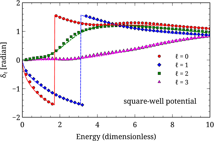
Figure 1: The scattering phase shift from the square-well potential as a function of (dimensionless) energy. The symbols are the scattering overlap relation (SOR) results for orbital angular momentum $\ell$ from 0 to 3. We solved the Lippmann-Schwinger equation with $N_{\rm{pot}}=10$ and oscillator length $b=0.42$, which minimizes the ground state energy in this truncated space. The lines are analytic solutions. The well has dimensionless radius $R=1$ and depth $V_{0}=-5$; in addition, $\hbar=\mu=1$.

We work in a harmonic oscillator (HO) basis, that is, our $\phi_{n}(r)$ are 3-D harmonic oscillator radial wave functions. In coordinate space the regular and irregular free solutions are spherical Bessel functions $f(r)=kr\,j_{\ell}(kr)$ and spherical Neumann function $g(r)=kr\,y_{\ell}(kr)$, respectively; then the $f_{n}$ and $g_{n}$ have analytic expressions (see PhysRevC.94.064320 and references therein):

$$f_{n} = {\cal N}(n,\ell)q^{\ell+1}\exp(-q^{2}/2)L^{\ell+1/2}_{n}(q^{2}),$$ (38)

$$g_{n} = {\cal N}(n,\ell)\frac{-q^{\ell}}{\Gamma(-\ell+1/2)}\exp(-q^{2}/2)\,$$

$$\times\Phi(-n-\ell-1/2;-\ell+1/2;q^{2}),$$

where the overall normalization factor is given by

$${\cal N}(n,\ell)=\sqrt{\frac{\pi\Gamma(n+1)}{\Gamma(n+\ell+3/2)}},$$ (40)

with $q=\sqrt{\frac{2E}{\hbar\omega}}=kb$, and $\Phi$ is the confluent hypergeometric function. Here $n$ is the number of nodes in the radial wave function, related to the principal quantum number $N_{\mathrm{princ}}$ by $N_{\mathrm{princ}}=2n+l$. In applications, the confluent hypergeometric function can be numerically challenging for large values of the arguments muller2001computing ; pearson2017numerical . Finally, we found the scattering solutions $u_{n}$ by solving the LS equation (37); although not shown, separate calculations of the $u_{n}$ found by matrix diagonalization gave very good agreement. The LS equation, however, allowed for finer sampling of the continuum.

Our first example is scattering off a square well potential, for which analytic solutions are easily found. For Fig. 1 we chose dimensionless parameters $\hbar=\mu=1$, potential well radius $R=1$, and well depth $V_{0}=-5$. We choose $N_{\mathrm{pot}}=10$ and used a harmonic oscillator length parameter, $b=b_{\mathrm{min}}=\sqrt{\hbar/\mu\omega}=0.42$, where $\omega$ is the oscillator frequency. This choice of $b$ minimizes the ground state energy in this truncated space; in the Appendix, we discuss the relation between the ground state energy and the quality of the phase shifts. In a large harmonic oscillator basis ($N_{\mathrm{pot}}=200$) the dimensionless ground state energy is $-2.312$, with very little sensitivity to $b$, in agreement within numerical error with the result in coordinate space. Even in our smaller space, $N_{\mathrm{pot}}=10$, we get excellent agreement with the analytic phase shifts for orbital angular momentum $\ell=0,1,2,3.$

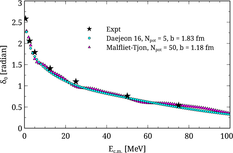
Figure 2: The isoscalar $s$-wave phase shifts using the Daejeon 16 potential (circles) with $N_{\rm{pot}}=5$, $b=1.83$ fm (which corresponds to $\hbar\omega=25$ MeV), and the Malfliet-Tjon potential (triangles) with $N_{\mathrm{pot}}=50$ ($b=b_{\rm{min}}$ = 1.18 fm, $E_{\rm{g.s.}}=-2.287$ MeV). Experimental values PhysRevC.48.792 are stars. We excluded coupling to ${}^{3}D_{1}$ partial wave in the calculation with Daejeon-16, resulting in a ground state energy of -1.022 MeV.

For a more realistic, and more challenging, case, we computed isoscalar ${}^{3}S_{1}$ nucleon-nucleon phase shifts. In Fig. 2, we compare against experimental phase shifts PhysRevC.48.792 results using two interaction models. The first is the Malfliet-Tjon potential malfliet1970three :

$$V_{\mathrm{MT}}(r)=V_{a}\frac{e^{-\mu_{a}r}}{r}+V_{r}\frac{e^{-\mu_{r}r}}{r},$$ (41)

with parameter values $V_{a}=-635$ MeV, $V_{r}=1458$ MeV, $\mu_{a}=1.55$ fm^-1, and $\mu_{r}=3.11$ fm^-1. These parameters yield a deuteron binding energy of $-2.29$ MeV, in rough agreement with experimental value $-2.22$ MeV Greene1986 . The other is the more modern Daejeon-16 interaction shirokov2016n3lo , generated from chiral effective field theory interaction matrix elements PhysRevC.68.041001 and softened through the similarity renormalization group and phase-equivalent transformations. Daejeon-16 exists only as matrix elements in harmonic oscillator space.

We computed the SOR phase shifts from Daejeon-16 in a small space, $N_{\mathrm{pot}}=5$, using a harmonic oscillator length parameter $b=1.83$ fm, which corresponds to a frequency of $\hbar\omega=25$ MeV. Because we leave the coupled-channel formalism to future work, we excluded the coupling to the ${}^{3}D_{1}$ partial wave, which led to a poor value of the ground state energy, $-1.022$ MeV (if we include the ${}^{3}D_{1}$ we regain a good value of the ground state energy), but nonetheless get good agreement with experimental phase shifts. We believe the soft nature of Daejeon-16 is important, because the Malfliet-Tjon interaction, with a strong repulsive core, proved more challenging. In Fig. 2, using $N_{\mathrm{pot}}=50$ and a $b_{\mathrm{min}}=1.18$ fm, we obtained the general trend of the experimental phase shifts, albeit with some slight oscillations, which are not seen for phase shifts computed in coordinate space. If we use a smaller $N_{\mathrm{pot}}$, however, the oscillations seen in Fig. 2, grow in amplitude.

These examples demonstrate our novel SOR formula for calculations in an $L^{2}$-integrable basis satisfactorily reproducs phase-shifts for single-channel potential scattering. In some cases we can achieve this with a relative small model space; however for the Malfliet-Tjon potential, which has a strong repulsive core, we required a larger space for satisfactory results.

V Conclusions

We have derived a generalized scattering overlap relation (SOR) which applies to both continuous position basis calculations and to discrete, $L^{2}$-integrable bases such as the harmonic oscillator basis used in $J$-matrix calculations, and demonstrated we can apply the discrete SOR to various potentials, including at nonzero angular momentum. In some cases we reproduce the phase shifts in a relatively small model space, in particular for a soft interaction such as Daejeon-16. We found conversely that the Malfliet-Tjon potential, which has a strong short-range repulsive core, required a larger model space. In the Appendix, we discuss the relation between reproducing phase shifts and reproducing the ground state energy.

In the near future we will generalize to coupled-channel calculations, asymptotic normalization coefficients, and Coulomb scattering. While SORs have been used before in position basis calculations, we plan to apply our generalization to many-body frameworks using square-integrable bases.

Appendix A Truncation, phase shifts, and the ground state energy

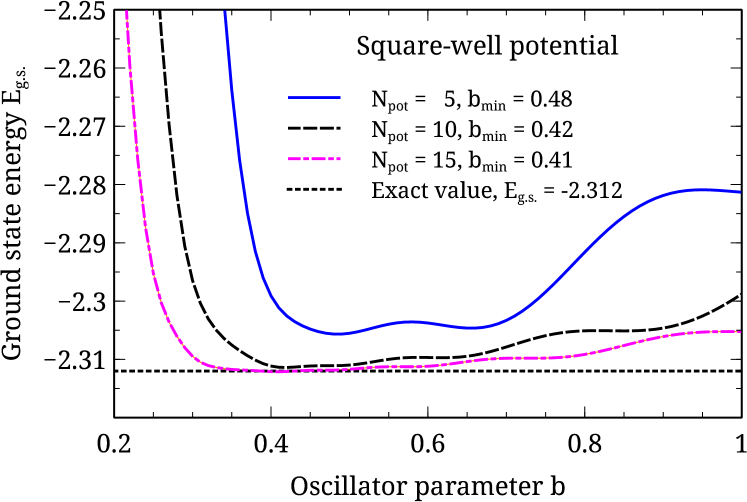
Figure 3: The ground state energy of the system when the parameter $b$ is varied. The exact value of the ground state energy (horizontal line) is $-2.312$ (dimensionless). $b_{\rm{min}}$ is the value that makes $E_{\mathrm{g.s.}}$ minimum.

Out of practicality, one must truncate the matrix representation of the potential $V_{n,n^{\prime}}$, such that $n,n^{\prime}\leq N_{\mathrm{pot}}$. In tractable many-body calculations, the effective $N_{\mathrm{pot}}$ might be quite small: because of parity, an $N_{\mathrm{pot}}$ of 5 is equivalent to twelve oscillator shells in a no-core nuclear shell model calculation barrett2013ab . Nonetheless, our results demonstrate one can reasonably reproduce the phase shifts for such a small $N_{\mathrm{pot}}$, especially for a soft interaction such as Daejeon-16.

In the course of our investigation, we found the quality of the phase shifts correlated with the quality of the ground-state energy. (The cases we considered above each had exactly one bound state.) Specifically, for a fixed $N_{\mathrm{pot}}$, we varied the oscillator length parameter $b=\sqrt{\hbar/\mu\omega}$, where $\omega$ is the oscillator frequency. We found our ‘best’ phase shifts when $b$ minimized the (bound) ground state energy.

To demonstrate this, consider the same square well potential as in Fig. 1, which has a (dimensionless) ground state energy of -2.312 (that this is numerically similar to the deuteron’s binding energy in MeV is coincidental). In Fig. 3 we compute the ground state energy, that is, the energy of the single $s$-wave bound state, in a basis of oscillator states, as a function of the oscillator length parameter $b$ for $N_{\mathrm{pot}}$ = 5, 10, and 15.

Unsurprisingly, calculations in larger spaces (larger $N_{\mathrm{pot}}$) are less sensitive to $b$ and are closer to the infinite space ground state energy. (One can understand the sharp upturn at small $b$ by appealing to an important property of the oscillator functions: the classical turning point,

$$R_{cl}=b\sqrt{4N_{\mathrm{pot}}+2\ell+3}.$$ (42)

For $\ell=0$ and for $N_{\mathrm{pot}}=5$, we get approximately $R_{cl}\approx 4.8b$, so when $b<0.2$, the classical turning point is within the well radius. In such a case it is unsurprising the ground state energy is badly estimated.)

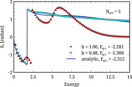
Figure 4: The scattering phase shift by the square-well potential with $N_{\mathrm{pot}}=5$. For $b=1.00$ and $0.48$, the bound state energies are $-2.281$ and $-2.306$ (dimensionless), respectively. The large-space ground state energy is -2.312.

Correlated with the ground state energy are the phase shifts. In Fig 4 we show the $s$-wave phase shift for $N_{\mathrm{pot}}=5$ and for two different values of $b$, compared with the exact analytic result. Note that the phase shift is improved when the ground state energy is better approximated, a general result we found in our investigations. While this is not surprising, we have not found an effective argument to link bound state energies and phase shifts. In many-body calculations in a harmonic oscillator basis barrett2013ab , one typically chooses the basis frequency (and thus the length parameter $b$), so as to minimize the ground state energy. This gives us hope that, even in a highly truncated basis, we can effectively recover scattering information. This will be part of future investigations.

References

- [1] Ernest Rutherford. The scattering of and particles by matter and the structure of the atom. Philosophical Magazine, 21:669–699, 911.
- [2] Walter Gloeckle, H Witała, D Hüber, H Kamada, and J Golak. The three-nucleon continuum: achievements, challenges and applications. Physics Reports, 274(3-4):107–285, 1996.
- [3] Walter Glöckle. The quantum mechanical few-body problem. Springer Science & Business Media, 2012.
- [4] F. Ciesielski and J. Carbonell. Solutions of the Faddeev-Yakubovsky equations for the four nucleon scattering states. Phys. Rev. C, 58:58–74, Jul 1998.
- [5] Calvin W Johnson, Kristina D Launey, Naftali Auerbach, Sonia Bacca, Bruce R Barrett, Carl R Brune, Mark A Caprio, Pierre Descouvemont, WH Dickhoff, Charlotte Elster, et al. White paper: from bound states to the continuum. Journal of Physics G: Nuclear and Particle Physics, 47(12):123001, 2020.
- [6] Eric J. Heller and Hashim A. Yamani. New approach to quantum scattering: Theory. Phys. Rev. A, 9:1201–1208, Mar 1974.
- [7] Eric J. Heller and Hashim A. Yamani. -matrix method: Application to s-wave electron-hydrogen scattering. Phys. Rev. A, 9:1209–1214, Mar 1974.
- [8] Abdulaziz D Alhaidari, Eric J Heller, Hashim A Yamani, and Mohamed S Abdelmonem. The J-matrix method. Development and Applications (Springer, Berlin, 2008), 2008.
- [9] Roger G Newton. Scattering theory of waves and particles. Springer Science & Business Media, 2013.
- [10] A. M. Shirokov, A. I. Mazur, I. A. Mazur, and J. P. Vary. Shell model states in the continuum. Phys. Rev. C, 94:064320, Dec 2016.
- [11] I. A. Ivanov, J. Mitroy, and K. Varga. Elastic positronium-atom scattering using the stochastic variational method. Phys. Rev. Lett., 87:063201, Jul 2001.
- [12] Tore Berggren. Overlap integrals and single-particle wave functions in direct interaction theories. Nuclear Physics, 72(2):337–351, 1965.
- [13] WT Pinkston and GR Satchler. Form factors for nuclear stripping reactions. Nuclear Physics, 72(3):641–656, 1965.
- [14] Leonard S Rodberg, Roy M Thaler, and Raphael Morton Thaler. Introduction to the quantum theory of scattering, volume 26. Academic Press, 1967.
- [15] NK Timofeyuk. One nucleon overlap integrals for light nuclei. Nuclear Physics A, 632(1):19–38, 1998.
- [16] Y Suzuki, W Horiuchi, and K Arai. Phase-shift calculation using continuum-discretized states. Nuclear Physics A, 823(1-4):1–15, 2009.
- [17] A. Kievsky, M. Viviani, Paolo Barletta, C. Romero-Redondo, and E. Garrido. Variational description of continuum states in terms of integral relations. Phys. Rev. C, 81:034002, Mar 2010.
- [18] Kenneth M. Nollett. Ab initio calculations of nuclear widths via an integral relation. Phys. Rev. C, 86:044330, Oct 2012.
- [19] Abraham R. Flores and Kenneth M. Nollett. Variational Monte Carlo calculations of scattering. Phys. Rev. C, 108:034001, Sep 2023.
- [20] RD Lawson. Theory of the nuclear shell model. Clarendon Press Oxford, 1980.
- [21] Thom H Dunning Jr and P Jeffrey Hay. Gaussian basis sets for molecular calculations. In Methods of electronic structure theory, pages 1–27. Springer, Boston MA, 1977.
- [22] Hashim A Yamani and Louis Fishman. J- matrix method: Extensions to arbitrary angular momentum and to Coulomb scattering. Journal of Mathematical Physics, 16(2):410–420, 1975.
- [23] V. S. Vasilevsky and F. Arickx. Algebraic model for quantum scattering: Reformulation, analysis, and numerical strategies. Phys. Rev. A, 55:265–286, Jan 1997.
- [24] JM Bang, AI Mazur, AM Shirokov, Yu F Smirnov, and SA Zaytsev. P-matrix and J-matrix approaches: Coulomb asymptotics in the harmonic oscillator representation of scattering theory. Annals of Physics, 280(2):299–335, 2000.
- [25] H. A. Yamani, A. D. Alhaidari, and M. S. Abdelmonem. J-matrix method of scattering in any basis. Phys. Rev. A, 64:042703, Sep 2001.
- [26] Eric J. Heller. Theory of -matrix Green’s functions with applications to atomic polarizability and phase-shift error bounds. Phys. Rev. A, 12:1222–1231, Oct 1975.
- [27] John T. Broad and William P. Reinhardt. One- and two-electron photoejection from H-: A multichannel -matrix calculation. Phys. Rev. A, 14:2159–2173, Dec 1976.
- [28] J Révai, M Sotona, and J Zofka. Note on the use of harmonic-oscillator wavefunctions in scattering calculations. Journal of Physics G: Nuclear Physics, 11(6):745, 1985.
- [29] V. Vasilevsky, A. V. Nesterov, F. Arickx, and J. Broeckhove. Algebraic model for scattering in three--cluster systems. i. theoretical background. Phys. Rev. C, 63:034606, Feb 2001.
- [30] Yu A Lurie and Andrey M Shirokov. Loosely bound three-body nuclear systems in the J-matrix approach. Annals of Physics, 312(2):284–318, 2004.
- [31] A. M. Shirokov, A. I. Mazur, S. A. Zaytsev, J. P. Vary, and T. A. Weber. Nucleon-nucleon interaction in the -matrix inverse scattering approach and few-nucleon systems. Phys. Rev. C, 70:044005, Oct 2004.
- [32] J Broeckhove, Frans Arickx, P Hellinckx, VS Vasilevsky, and AV Nesterov. The 5H resonance structure studied with a three-cluster J-matrix model. Journal of Physics G: Nuclear and Particle Physics, 34(9):1955, 2007.
- [33] A. M. Shirokov, A. I. Mazur, J. P. Vary, and E. A. Mazur. Inverse scattering -matrix approach to nucleon-nucleus scattering and the shell model. Phys. Rev. C, 79:014610, Jan 2009.
- [34] IA Mazur, AM Shirokov, AI Mazur, and JP Vary. Description of resonant states in the shell model. Physics of Particles and Nuclei, 48:84–89, 2017.
- [35] A. M. Shirokov, A. I. Mazur, I. A. Mazur, E. A. Mazur, I. J. Shin, Y. Kim, L. D. Blokhintsev, and J. P. Vary. Nucleon- scattering and resonances in 5He and 5Li with JISP16 and Daejeon16 interactions. Phys. Rev. C, 98:044624, Oct 2018.
- [36] AI Mazur, AM Shirokov, IA Mazur, LD Blokhintsev, Y Kim, IJ Shin, and JP Vary. Description of continuum states within the no-core shell model: single-state HORSE method. Physics of Atomic Nuclei, 82:537–548, 2019.
- [37] AM Shirokov, AI Mazur, IJ Shin, Y Kim, P Maris, and JP Vary. Description of continuum spectrum states of light nuclei in the shell model. Physics of Particles and Nuclei, 50(5), 2019.
- [38] I. A. Mazur, I. J. Shin, Y. Kim, A. I. Mazur, A. M. Shirokov, P. Maris, and J. P. Vary. SS-HORSE extension of the no-core shell model: Application to resonances in . Phys. Rev. C, 106:064320, Dec 2022.
- [39] Yu A Lashko, VS Vasilevsky, and GF Filippov. Properties of a potential energy matrix in oscillator basis. Annals of Physics, 409:167930, 2019.
- [40] Konstantinos Kravvaris and Alexander Volya. Clustering in structure and reactions using configuration interaction techniques. Phys. Rev. C, 100:034321, Sep 2019.
- [41] B. V. Noumerov. A Method of Extrapolation of Perturbations. Monthly Notices of the Royal Astronomical Society, 84(8):592–602, 06 1924.
- [42] B. Numerov. Note on the numerical integration of d2x/dt2 = f(x, t). Astronomische Nachrichten, 230(19):359–364, 1927.
- [43] A. M. Lane and R. G. Thomas. R-matrix theory of nuclear reactions. Rev. Mod. Phys., 30:257–353, Apr 1958.
- [44] Abraham R. Flores and Kenneth M. Nollett. Variational Monte Carlo calculations of scattering. Phys. Rev. C, 108:034001, Sep 2023.
- [45] Keith E Muller. Computing the confluent hypergeometric function, . Numerische Mathematik, 90(1):179–196, 2001.
- [46] John W Pearson, Sheehan Olver, and Mason A Porter. Numerical methods for the computation of the confluent and Gauss hypergeometric functions. Numerical Algorithms, 74(3):821–866, 2017.
- [47] V. G. J. Stoks, R. A. M. Klomp, M. C. M. Rentmeester, and J. J. de Swart. Partial-wave analysis of all nucleon-nucleon scattering data below 350 MeV. Phys. Rev. C, 48:792–815, Aug 1993.
- [48] RA Malfliet and JA Tjon. Three-nucleon calculations with realistic forces. Annals of Physics, 61(2):425–450, 1970.
- [49] G. L. Greene, E. G. Kessler, R. D. Deslattes, and H. Börner. New determination of the deuteron binding energy and the neutron mass. Phys. Rev. Lett., 56:819–822, Feb 1986.
- [50] AM Shirokov, IJ Shin, Y Kim, M Sosonkina, P Maris, and JP Vary. N3lo nn interaction adjusted to light nuclei in ab exitu approach. Physics Letters B, 761:87–91, 2016.
- [51] D. R. Entem and R. Machleidt. Accurate charge-dependent nucleon-nucleon potential at fourth order of chiral perturbation theory. Phys. Rev. C, 68:041001, Oct 2003.
- [52] Bruce R Barrett, Petr Navrátil, and James P Vary. Ab initio no core shell model. Progress in Particle and Nuclear Physics, 69:131–181, 2013.