1.4pt
††institutetext: * Center for Nuclear Theory,
SUNY, Stony Brook, NY 11794, USA
** C.N. Yang Institute for Theoretical Physics,
SUNY, Stony Brook, NY 11794, USA
Weinberg Institute,
The University of Texas at Austin, TX 78712, USA
A stress tensor for asymptotically flat spacetime
Abstract
In this article, we propose a procedure for calculating the boundary stress tensor of a gravitational theory in asymptotic flat spacetime. As a case study, the stress tensor correctly reproduces the Brown-York charges for Kerr blackhole i.e. mass and angular momentum. In asymptotic flat spacetime, there are asymptotic symmetries called BMS symmetries. We also compute the charges associated with these symmetries with the proposed stress tensor. The asymptotic charges can be compared with the Wald-Zoupas method. Our result for the stress tensor can be interpreted as the expectation value for the boundary stress tensor.
YITP-SB-2024-33
1 Introduction and summary
Gravity in any spacetime is believed to be holographic. The Hamiltonian of gravity is a boundary term (on-shell). One can even say holography is implicit in canonical gravity Raju:2019qjq . This fact about canonical gravity is immensely enriched by our understanding of gravity in asymptotically Anti-de-Sitter (AdS) spacetime Witten:1998qj ; Aharony:1999ti ; Maldacena:1997re . The dictionary between the bulk fields living in AdS and corresponding boundary operators has been established. In particular, the gravitons in the AdS spacetime are dual to the stress tensor on the boundary CFT. Hence, the stress tensor for boundary CFT can be obtained using the holographic method. The stress tensor obtained this way is the stress tensor of its respective spacetime. In asymptotic AdS spacetime, Balasubramanian and Kraus Balasubramanian:1999re used the variational principle and suitable counter terms to find the stress tensor. Then they used it to compute the conserved charges (Brown-York) for isometries of spacetime Brown:1992br like mass and angular momenta. Furthermore, CFT in even dimensions often has conformal and Weyl anomalies. These anomalies have been efficiently computed using holographic methods (see Bianchi:2001kw ; Skenderis:2002wp ; Henningson:1998gx ; deHaro:2000vlm for some of the early papers). In particular, They showed the central charge of the 2d CFT is proportional to 3d AdS length scale in Plancks unit Brown:1986nw .
| (1) |
This relation has been achieved by finding the transformed stress tensor for AdS3 spacetime upon the action of asymptotic symmetries and comparing it with the transformation rule for the boundary stress tensor. The asymptotic symmetries of AdS3 spacetime are the Virasoro symmetries of the 2d CFT. In AdS, these holographic methods lead to many developments in understanding CFT in general. The monotonic c and a theorems were first established using holographic methods Myers:2010tj ; Myers:2010xs then proven in QFT by Komargodski et al. Komargodski:2011vj (a-theorem). See recent work by Karateev et al. Karateev:2023mrb for bounding the along the RG flows. The entanglement entropy in 2d CFT is first calculated by Calabrese et al. Calabrese:2004eu and then reproduced by Ryu et al. Ryu:2006ef in all dimensions using the holographic methods. These are some of the avenues ripe for holographic calculation in flat spacetime.
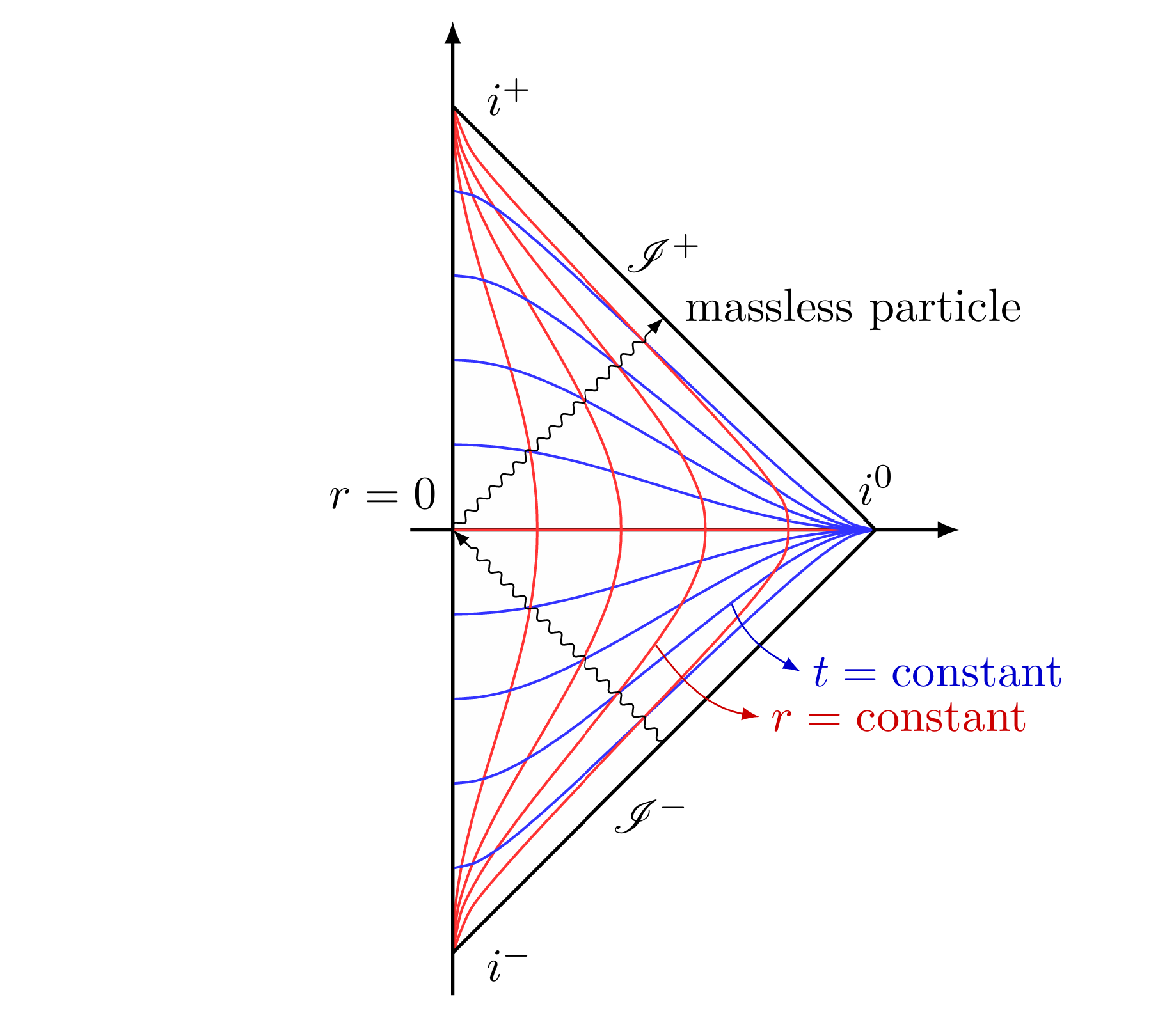
These ideas from the AdS can be borrowed and applied to the flat spacetime. The conformal structure of flat spacetime (Fig.1) is more complicated than AdS spacetime. There are two null hypersurfaces, . Massless particles come from past null infinity, , and go to future null infinity, . While massive particles start from and end at . Finally, there’s spatial infinity . Here one often does anti-podal matching of incoming and outgoing data Strominger:2017zoo . In this article, we will focus only on the future null infinity, where gravitons and other massless particles finally end up. The stress tensor at null infinity can be understood in a similar way. The stress tensor at and and its relation to the stress tensor at null infinity are left for future exploration (similar in the spirit of Ashtekar:2023wfn ; Ashtekar:2023zul ).
In general relativity, one often needs to add a boundary term to make the variational principle well-defined. For the AdS spacetime, the trace of extrinsic serve the purpose. This is also called the Gibbons-Hakwing-York term. This makes the variational principle well defined but the stress tensor obtained from variation is often divergent. Balasubramanian et al.Balasubramanian:1999re have added suitable counterterms made from the induced metric and its curvature. Then they obtained a finite stress tensor and finite conserved charges. We will follow the same logic. But in the asymptotic flat case, the boundary is null rather than time like. Hence, for an asymptotically flat spacetime (the boundary is null) one requires a different boundary term. In this case inaffinity fits the bill Parattu:2015gga ; Chandrasekaran:2020wwn ; Chandrasekaran:2021hxc ; Aghapour:2018icu ; Jafari:2019bpw . Inaffinity is the failure of the null vector to be affinely parameterized.
| (2) |
for the null vector .
Upon the variation of the boundary term, we have a candidate expression for the stress tensor. It is given by the Weingarten tensor and its traces.
| (3) |
Where the Weingarten tensor is calculated by the covariant derivative of the normal vector and pulled back to the null surface.
| (4) |
The projectors are used to pull back the bulk quantity on the null surface . The covariant derivative uses the usual Levi-Civita connection of the bulk spacetime. We explicitly evaluate the stress tensor 111The stress tensor calculated via this way is finite. for asymptotically flat spacetime which has parameters like Bondi mass aspect , Angular momentum aspect , shear and Bondi-News . Then we used the stress tensor to compute the conserved charges for global and asymptotic symmetries. Although the charges corresponding to the BMS symmetries have been calculated via different methods like the covariant phase space method (Wald-Zoupas)Wald:1999wa ; Barnich:2011mi and by Ashetaker et al. using Hamiltonian formulation Ashtekar:2024bpi ; Ashtekar:2024mme ; Ashtekar:2024stm . But we find it useful to find these charges from the Brown-York procedure which requires a definition of stress tensor. The holographic stress tensor will become the stress tensor of the Carrollian QFT living at the boundary. This is the main motivation for our work. We obtain the conserved charges like mass and angular momentum for Schwarzchild and Kerr Blackholes. For the asymptotic symmetries (BMS symmetries), We also find the conserved charges. These charges are a little different from the Wald-Zoupas charges Donnay:2022wvx ; Barnich:2011mi that already exist in the literature222For the general formalism for Wald-Zoupas formalism see Wald:1984rg ; Wald:1999wa .. Explicitly we have
The discrepancy lies only in the first term. In the first term, the Wald Zoupas charge has dependence . The news dependence term in the charges is non-integrable. Hence, we are not able to reproduce the non-integrable charges. Wald Zoupas charge matches with Brown-York charge up to a scaling anomaly Chandrasekaran:2021hxc ; Chandrasekaran:2020wwn . There are additional counterterms whose variations can account for the discrepancy. The scaling anomaly and suitable counterterms are left for future work.
We have also computed the Brown-York charges for the Kerr Blackhole and correctly reproduced the mass and angular momentum (see section 5.1 for more details.) For angle-dependent symmetries, we have found charges compatible with Barnich et al. Barnich:2011mi
Structure of the article: In section 2, we review the construction for the AdS spacetime which will set the stage for the flat case. In section 3, we review the Carrollian structure at null infinity with an emphasis on how these structures are induced from the bulk. This set the stage for the choice of boundary term required for the well-defined variational principle. Then in section 4, we use the variational principle to construct a candidate stress tensor suitable for null surfaces in terms of Weingarten tensor. In section 4.3, we compute the stress tensor of asymptotic flat spacetime . In section 5, we evaluate Brown-York charges of BMS symmetries. In section 5.1, we do the explicit evaluation for charges for the Kerr black hole. Some of the discussions about null hyper surfaces are relegated to appendix A.
Notation: The beginning of the alphabet are used to denote the spacetime bulk indices (4d). The middle of the alphabet are used for the null hypersurface (3d) indices. Capital letters are reserved as indices for the round metric on the or . Vectors and forms are denoted by unbold & bold letters, respectively e.g. vector k, and 1-form n. The spacetime volume form is denoted by and for the hypersurface it’s, . Carrollian vector is always defined as or while, the auxiliary null vector is denoted as or . There is an additional vector in the bulk which is the normal vector .
2 AdS spacetime: a warm-up and a sketch of the formalism
There are numerous ways to foliate a spacetime. In the ADM formalism, (i.e. Hamiltonian formulation of GR) one usually foliates spacetime with a family of a spacelike hypersurface at fixed time . One then constructs a Hamiltonian that generates the system’s time evolution between the spacelike hypersurfaces . In AdS, one usually foliates spacetime with timelike slices at fixed values of the radial coordinate. Pushing one of these slices to infinity (), one reaches the conformal boundary. Then, one can construct a stress tensor for AdS gravity by varying the gravitational action (along with boundary term) with respect to boundary metric. More explicitly
| (6) |
where is the gravitational action as a functional of the boundary metric .
The gravitational action for AdS spacetime is
| (7) |
The second term (the trace of extrinsic curvature) makes the variational principle well-defined. In AdS, the counter terms are often needed to make stress tensor and conserved charges finite. Then, the stress tensor upon varying the action Balasubramanian:1999re is
| (8) |
As an example, for AdS3 gravity the counter terms and stress tensor can be written as
| (9) |
Similar counter terms and stress tensors for higher dimensional AdS spacetime can be explicitly written. The stress tensor depends on the geometric structure (intrinsic as well extrinsic) of the boundary metric. Then AdS/CFT correspondence asserts the above stress tensor as an expectation value of the CFT stress tensor.
| (10) |
This relation connects the stress tensor computed using e.q. 6 with the CFT stress tensor, making the former holographic. In the above analysis, it was crucial that the authors of Balasubramanian:1999re foliated the spacetime by constant slices and then took limit. In this limit, the slice can be identified with the boundary.
3 Asymptotic flat spacetime: Null foliation
The asymptotically flat spacetime is a solution to Einstein’s equation with zero cosmological constant
| (11) |
The Penrose diagram of the flat spacetime is shown in fig 1. The boundary is null. We foliate the spacetime by constant slices 333There is another choice: the constant slices. These slices are null at any constant . (time-like) as shown by red lines in fig 1. When one takes the limit the slices can be identified with . But we will be interested only at the future null infinity.
3.1 Carrollian structure at null boundary:
A general solution of Einstein’s equation can be written in asymptotic expansion in Bondi gauge as (for most general solution see section 4.2)
| (12) | |||||
At null infinity, since , and we pull the conformal factor , then we have 444The in the expression below means the equality only at the null infinity.
| (13) | |||||
Here is the metric on the . The Carroll structure consists of a pair , where is the degenerate metric and is the normal vector in the kernel of metric as . For the Minkowski spacetime (setting all the parameters in the above metric to zero), the normal vector is . In the subsequent sections, we discuss how the Carroll structure gets induced from the bulk spacetime.
3.2 Induced Carroll structure on constant hypersurface
First, we review the formalism of induced Carroll structure on fixed hypersurface in bulk spacetime Freidel:2022bai ; Freidel:2022vjq . Next, we see how the Carroll structure on this hypersurface gets identified with the Carroll structure at null infinity when the hypersurface is pushed to the boundary. 555The formalism works for any null hypersurface but we are interested at null infinity.
We start with a 4d spacetime with a Lorentz signature metric and the Levi-Civita connection . We foliate this spacetime by a family of 3-dimensional timelike slices at fixed , called stretched Horizon(s) Riello:2024uvs ; Freidel:2024emv . is parametrized by . Next, we equip with an extrinsic structure called the rigged structure (explained below). The Carroll structure is then induced from the rigged structure and more importantly it becomes an intrinsic structure on . After pushing the slice to the boundary, this Carroll structure gets identified with the Carroll structure at (see Donnay et al.Donnay:2019jiz for similar construction at the black hole horizon). Let’s discuss some definitions.
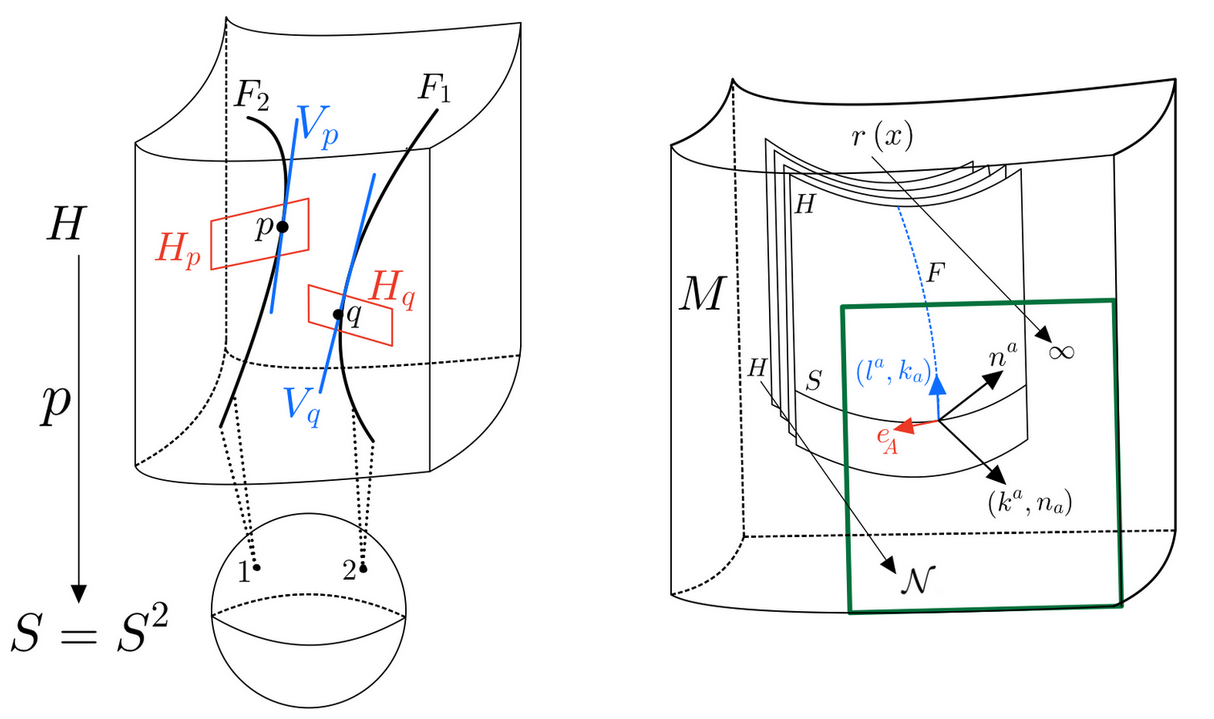
Carroll structure: The Carrollian Viewpoint consists of splitting the tangent space of the stretched horizon into vertical & horizontal subspaces 666This is useful when this slice is pushed to where this decomposition helps to isolate the null direction in the subspace, from the remaining directions in . (See fig 2 for more details) so that the entire tangent bundle decomposes as
| (14) |
We begin by treating the stretched horizon as a line bundle , where the base space and the 1-dimensional fiber is attached to each point on . is spanned by a Carrollian vector ) (which is tangent to and points along the fibre see fig.2 right panel). Thus defines the . Next, we introduce the Ehresmann connection 1-form k which helps in defining by constructing a basis 777Remember that A is an index on hence runs over 1,2 or with respect to k such that . Basis spans . By construction, the Ehresmann connection 1-form k is dual to the Carrollian vector i.e. . Next, we can chart with local coordinates and a round metric . The null Carrollian metric on is defined as a pull-back of the round metric onto i.e. making it’s kernel i.e. . The collection is called the Carroll structure.
Null rigged structures: To understand the geometry of , we use the rigging technique developed by Mars and Senovilla Mars_1993 . This involves embedding the stretched horizons in spacetime using the foliation . Due to embedding, there is a natural notion of a normal 1-form, , where . A rigging vector field, is then introduced which is transverse to and is the dual to the normal 1-form, . The pair of dual rank-1 tensors is known as the rigged structure (fig.2 right panel).
Now we introduce a projection operator that will project all tensors defined in into . The rigged projection tensor, is defined as,
| (15) |
As an example, if and , then and . These projected tensor satisfies .
To treat timelike and null surfaces simultaneously one often chooses the rigging vector to be null by requiring Freidel:2022vjq , where . Thus, we have making a null rigging vector,
| (16) |
Thus the pair with being a null vector, defines the null rigged structure on . The final piece of ingredient is a tangential vector field and whose components are given by,
| (17) |
One can check that . With these properties, it is evident that could be thought as of a Carrollian vector 888Note that even though we introduced while constructing the null rigged structure and later identified it with the Carrolian vector, it’s not a null vector in the embedding space, (as opposed to which is a null vector in ), rather is a null vector strictly on . and becomes the Ehresmann connection. The normalization from (17) captures the idea of stretching of H, in the spirit that if then the metric defines as a timelike surface while when the metric defines as a null surface. As , hence . With the help of and k when needed we can decompose the rigged projection tensor into horizontal and vertical bases to provide the Carrollian viewpoint
| (18) |
Here is the projector onto the horizontal subspace i.e. . The degenerate metric on the can be found as . This is an important result, hence we will summarize what we have done so far.
Result: Given a null rigged structure on an embedded stretched horizon and the embedding spacetime metric the Carroll structure gets naturally induced on where
| (19) |
The vectors span the tangent space while 1-forms span the cotangent space . The spacetime metric is decomposed into the horizontal, vertical, and radial directions as
| (20) | |||||
Next, the rigged metric and its dual can be written with the help of projection tensor
| (21) | |||
| (22) |
A rigged connection on is simply the projection of the Levi-Civita connection on from
| (23) |
here is any tensor field defined on . This rigged connection is torsion-free and preserves the rigged projection tensor (see section 2.5 of Freidel:2022vjq for more details.) however, the rigged metric is not covariantly constant with respect to the rigged connection. instead, it is proportional to the extrinsic curvature of
| (24) |
where is the extrinsic curvature, sometimes called the rigged extrinsic curvature. In similar spirit, the volume form on can be obtained from the volume form of spacetime by contraction with the null rigging vector i.e. .
3.3 Intrinsic and extrinsic geometry at null infinity
We have established that one can induce a Carrollian structure from the null rigid structure defined on . Moreover, this structure persists as we take i.e .
Let’s first understand the intrinsic geometry of the null infinity which has coordinates with indices , and . At null infinity, the geometry consists of degenerate metric and a preferred vector which is in the kernel of metric i.e. . These objects define a weak Carroll structure on the null infinity . The volume form on horizontal space ( which has metric ) is labeled by and the total volume form on is denoted as satisfies the following relations.
| (25) |
Here is called expansion, is the extrinsic curvature (although completely determined by intrinsic data ), and is the shear. The shape operator or Weingarten tensor of the null boundary describes the extrinsic data. It can be written as
| (26) |
Here we have used a mix index projection tensor which is useful for projecting the spacetime tensors (with index ) onto which has index as
| (27) |
The Carrollian vector and the Ehresmann connection on are 999as . But we keep using the as Carrollian vector on the null infinity. and respectively.
The Weingarten tensor satisfies the following identities
| (28) |
The preferred vector is the eigenvector of the Weingarten tensor with eigenvalues called inaffinity. The vector is null and hence generates the null geodesic on which satisfies the geodesic equation as
| (29) |
As before, the projection tensor can be used to define a rigged connection on from the spacetime Levi-Civita connection Mars_1993 as
| (30) |
This connection is torsionless but not compatible as
| (31) | |||
| (32) |
The connection can also act on covariant vectors as
| (33) |
The auxiliary vector relative to such that . With this one form, one can also define a projector on the horizontal forms as
| (34) |
This also helps us in defining the inverse metric as The shape operator can be decomposed as
| (35) |
Here and is called rotation one form which is defined by
| (36) |
here is Hájíček one form.
4 Stress tensor
In this section, We find the expression for the holographic stress tensor from the variation of gravitational action.
4.1 Gravitational action and variational principle
The gravitational action with boundary term is given
| (37) |
The invariant volume form on the boundary is denoted as . The variation of the action (37) with respect to boundary metric and normal vector is
The action variation is zero whenever the equation of motion is satisfied and the Carroll structure is fixed. The derivation of the above equation (4.1) is explicitly carried out in Chandrasekaran:2020wwn ; Parattu:2015gga . The on-shell classical action should be thought of as a functional of Carroll structure .
Then the variation of the action with parameter which changes the boundary metric as and normal vector as is
| (39) | |||
| (40) |
The expressions above can be rearranged as
| (41) |
The choice of can be made unambiguously. This decomposition defines the stress tensor by and . In terms of undensitized momenta (excluding the volume form) which is defined as , the stress tensor and generalized divergence are
| (42) | |||
| (43) |
The above expression for stress tensor can now be written in terms of Weingarten tensor as
| (44) |
This is the analog of the stress tensor obtained in AdS space using extrinsic curvature (see section 2 for a summary). In the flat space (with a null boundary), the shape operator (Weingarten tensor) plays the role of extrinsic curvature. The is independent of the choice of auxiliary vector and then mixed index tensor is independent of . Other index tensors like or might depend on the choice of . The stress tensor can be shown to be covariantly conserved on the boundary Chandrasekaran:2021hxc .
| (45) |
The first equality is obtained using the eq. (31). The second equality above can be obtained using the Codazzi equation for the null surfaces Gourgoulhon:2005ng ; Chandrasekaran:2021hxc . It is also established in Chandrasekaran:2021hxc that the transformation that acts covariantly on the boundary, the Brown York charges (calculated using stress tensor) matches with the Wald-Zoupas procedure.
4.2 Solutions of Einstein equation
Einstein’s equation in flat spacetime is . A general solution of Einstein’s equation in Bondi-gauge with coordinates as has the following asymptotic expansion in the large limit Donnay:2022aba ; Donnay:2022wvx ; Strominger:2017zoo ; Barnich:2011mi ; Barnich:2010eb .
| (46) |
Here the various parts of the above metric are
| (47) |
is a symmetric traceless tensor and other tensors are raised and lowered by the and its inverse. The news tensor is defined as and
| (48) | |||
| (49) |
Then we have as101010Often in and there is a logarithmic term like and its coefficients are . But here we are not including those terms. See Barnich:2011mi ; Barnich:2010eb for more details.
| (50) |
Here is the covariant derivative with respect to and is called the angular momentum aspect. The Ricci scalar is
| (51) |
Here is the Laplacian of the metric . The Einstein equation and are constraint equations and give the evolution of mass and angular momentum aspects.
| (52) | |||
| (53) |
Hence, the solution space is parametrized by
| (54) |
The metric on the boundary is often taken to be the round 2 sphere metric.
| (55) |
In this article, we will take the flat metric on the boundary as
| (56) |
This parametrization is often useful when doing explicit calculations. However, similar conclusions can be reached for other metrics as well. Let’s first take the example of Minkowski spacetime in this parametrization. We start with the following redefinition of coordinates as
| (57) |
Here all are usual Bondi coordinates. One can also relate this new coordinate to Cartesian ones as
| (58) |
After the redefinition, the Minkowski metric at is
| (59) |
We notice that the metric component by this redefinition. Similarly at past null infinity, one can redefine the coordinate and the metric in advanced coordinates is
| (60) |
At finite , One can make the following identification between these choices of the coordinate system
| (61) |
The Carrollian nature is more transparent in these flat boundary coordinate systems. At null infinity, we have and then the metric is
| (62) |
This is the degenerate metric at . The Carrollian vector is . After doing the coordinate transformation, the metric on the boundary is flat metric . This completes the analysis for Minkowski spacetime.
4.3 Stress tensor for flat boundary metric
Now for any asymptotic flat spacetime that has parameters like , etc, we will take the flat boundary representative instead of sphere (see Compere et al Compere:2016hzt ; Compere:2018ylh ; Barnich:2016lyg ; Donnay:2021wrk ; Donnay:2022wvx for more details).
| (64) | |||||
where the .
These parameters satisfy the following constraint equations. These constraints equations are components of Einstein tensor and .
| (65) |
| (66) |
where
The first and second equations can be interpreted as the decay of Bondi-mass and angular momentum aspects in the Bondi news (which is the gravitational radiation).
The boundary term inaffinity on these solutions can be explicitly obtained for the choice of written below.
| (67) |
Then the on-shell gravitational action is
| (68) |
Using the constraint Einstein above, The on-shell action is the dynamical mass of the system.
The null rigged structure that decomposes the metric into horizontal and tangential parts are
The form of is determined by the following decomposition111111It is important to have explicit term in . Then only we get the charges that are consistent with the Wald-Zoupas method..
| (70) |
Here is the metric on horizontal space. At the , this is metric on transverse space 121212This metric is degenerate in limit.. These are the “normal” () and auxiliary vector . The exact form of is a little complicated to write down but one can do the expansion in . Using the projection operator , the projection of the normal vector along the null surface defines the Carrollian vector.
The lower component is obtained using the metric as . The decomposition of inverse metric in terms of horizontal, and vertical parts can be written as
| (71) |
We can also define a projector that has mixed indices namely spacetime indices and indices along the null surface.
With these projectors, we can write down the Weingarten tensor on the null boundary as
| (72) |
The stress tensor can be computed as
The stress tensor components fall off like except for two components which have dependence. These would be relevant for understanding the stress tensor due to gravitons in flat spacetime. The where will be used for computing the Brown-York conserved charges (see section 5).
Trace of stress tensor:
The trace of stress tensor can be written as
| (74) |
The stress tensor is not traceless. Its relation to any anomaly of the boundary theory is not clear to us.
5 BMS Symmetries and charges
In this section, we will find the Brown York charges corresponding to the symmetries of the asymptotic form of the solution. The metric when written in Bondi gauge has supertranslation and superrotation symmetries. The vector field generating these symmetries can be written as Bondi:1962px ; Newman:1966ub ; Barnich:2011mi ; Madler:2016xju ; Strominger:2017zoo
| (75) | |||||
The above vector field 131313It is crucial to keep the terms in the part of the Killing vector field. Then only one can show that this is a Killing (conformal) vector field. generates symmetries at asymptotic infinity in the expansion. The parameters are called the supertranslation parameter while are the superrotation parameters. One can understand these symmetries as the conformal symmetries of the Carrollian structure at null infinity.
To understand the conformal symmetries for the Carrollian structure at the null boundary, let’s start from the Minkowski spacetime metric. The Carrollian structure is described by a degenerate metric and vector field in the kernel of . Here the index . The degenerate line element can be written as
| (76) |
The conformal Carrollian symmetries are generated by vector field
| (77) |
which satisfies the Carrollian conformal equation
| (78) |
This conformal Carrollian vector is the restriction of vector field of (75) to the null infinity in the leading order and taking the boundary metric to be the complex plane.
The Quasilocal charges for the supertranslation and superrotations symmetries can be calculated by the Brown York method using the stress tensor.
We have used the volume element at null infinity where and the spatial volume element . The dotted terms are of the order and will vanish in strict limit.
The charges (Wald- Zoupas) for BMS symmetries have been calculated using the covariant phase space method Barnich:2011mi ; Donnay:2022wvx .
| (80) |
The refined angular momentum aspect can be written as
| (81) |
The charges (Wald-Zoupas) for BMS symmetries are a little different than those of Brown York charges that we have obtained. The discrepancy lies only in the first term. In summary, we have a different non-integrable charge. To match these charges one needs counter terms whose variations give contribution to the stress tensor components. Wald Zoupas charge matches with Brown-York charge up to a scaling anomaly Chandrasekaran:2021hxc ; Chandrasekaran:2020wwn . The explicit dependence for the Brown York charge obtained in (5) can be found by find the flux as in section 5.5.2 of Compere:2018ylh .
Discussion of corner terms:
In this whole formalism, there are corner terms that we have ignored and there are choices of boundary terms (on the null boundary) that can change the corner terms. One of the choices is . Here is the expansion. These choices change the corner terms. These corner terms are integrated over co-dimension 2 surfaces.
| (82) | |||
| (83) |
5.1 Kerr Blackholes: A case study
The Kerr metric, which describes a rotating black hole in Boyer-Lindquist coordinates, is given by:
| (84) |
where the functions and are defined as:
| (85) | ||||
| (86) |
Here, is the mass of the black hole, and is the specific angular momentum per unit mass.
Now we write the metric in BMS gauge following SJFletcher:2003 ; Barnich:2011mi , This gives the various metric components as
| (87) | |||
| (88) | |||
| (89) | |||
| (90) | |||
| (91) | |||
| (92) | |||
| (93) |
Now the parameters of the asymptotic flat spacetime can be read off as
| (94) | |||
| (95) | |||
| (96) |
The normal and auxiliary vector for the Kerr spacetime () can be written as
| (97) | |||
| (98) |
These vectors are fixed by the following decomposition of the metric 141414Here the extra term of is needed because the . With that, the metric can be decomposed in terms of horizontal vertical, and transverse subspaces. In previous cases of asymptotic flat spacetime, the norm of the normal vector is hence, it was not needed where the metric goes most . To avoid this subtlety, one can do the coordinate transformation like the one done in (57). This will get rid of in the term. And then we don’t need to subtract the extra term.
| (99) |
With these normal vectors, we can compute the Weingarten tensor and then the stress tensor.
| (100) |
The stress tensor can be computed as
All other components are which are not relevant for the computation of charges or boundary stress tensor.
Brown York charges for the Kerr Blackhole
The vector fields generating the symmetries for the Kerr black hole is
| (102) |
Hence, the Brown York charges are
We have used the volume element at null infinity and the spatial volume element . The in the above equation are and won’t contribute to the charges. The global charges when and are independent of angular coordinates, then the Brown York charges gives the familiar mass and angular momentum of Kerr Blackholes. 151515The overall sign for the charges are consistent with Barnich:2011mi ; Wald:1999wa .
We can decompose the Killing vectors in spherical harmonics and find charges for each mode.
| (104) |
Only modes of the supertranslation will give the non-vanishing charge because the integral of spherical harmonics over the whole sphere is zero except for mode. For superotations, it is more convenient to transform to the complex coordinates () coordinates.
| (105) |
Then we can decompose these vector fields as
| (106) |
Then we can compute the charges for each mode as 161616The easiest way to do the following integrals is to transform it into angular variables using the stereographic map.
| (107) | |||
| (108) |
And the global charge for is . For the central extension of these algebras (see Barnich:2011mi section-4).
Acknowledgements.
The work of HK is party supported by NSF grants PHY-2210533 and PHY-2210562. J.B. is supported by the U.S. Department of Energy, Office of Science, Office of Nuclear Physics, grant No. DE-FG-02-08ER41450.Appendix A A gentle introduction to structure at null hypersurface
In this appendix, we reviewed the geometrical structure at the null surfaces borrowing intuition from the spacelike or time-like surfaces. We consider a 4-dimensional spacetime with Lorentzian signature metric . In this spacetime, a 3-dimensional hypersurface is defined via . A normal form to such a surface is . The sign depends of whether is timelike or spacelike, respectively. Then the normal vector is obtained using the inverse metric, . This definition of the normal form breaks down for null surfaces as the normalization becomes zero.
Instead, for the null surface we define
| (109) |
The sign is chosen so that is future-directed when increases to the future. Let’s evaluate
| (111) | |||||
where is the Levi-Civita connection. Note that everywhere on hence its gradient will be non-zero only away from the hypersurface i.e. in the direction of the normal hence the gradient of must be proportional to ,
| (112) |
where is some scalar function called inaffinity. Note that the normal vector field is tangent to . The normal vector satisfies the generalized geodesic equation (112). The hypersurface is generated by null geodesic and is tangent to the geodesic.
The null geodesics are parametrized parameter (not always affine). Then the displacement along the generator is . Then on , a coordinate system is placed that is compatible with generators. Hence, One of the coordinate is taken to be and two additional coordinates .
where A = 1, 2. The induced metric on the hypersurface can be written as
| (114) | |||||
On the null surface define an auxiliary vector satisfying and , with the help of which we decompose the inverse spacetime metric as,
| (115) |
where is the inverse of . Such null hypersurfaces with the above geometric structure are null infinity (see Poisson’s book Poisson_2004 - chapter 3 for an example and more details).
References
- (1) S. Raju, Is Holography Implicit in Canonical Gravity?, Int. J. Mod. Phys. D 28 (2019) 1944011 [1903.11073].
- (2) E. Witten, Anti-de Sitter space and holography, Adv. Theor. Math. Phys. 2 (1998) 253 [hep-th/9802150].
- (3) O. Aharony, S.S. Gubser, J.M. Maldacena, H. Ooguri and Y. Oz, Large N field theories, string theory and gravity, Phys. Rept. 323 (2000) 183 [hep-th/9905111].
- (4) J.M. Maldacena, The Large N limit of superconformal field theories and supergravity, Adv. Theor. Math. Phys. 2 (1998) 231 [hep-th/9711200].
- (5) V. Balasubramanian and P. Kraus, A Stress tensor for Anti-de Sitter gravity, Commun. Math. Phys. 208 (1999) 413 [hep-th/9902121].
- (6) J.D. Brown and J.W. York, Jr., Quasilocal energy and conserved charges derived from the gravitational action, Phys. Rev. D 47 (1993) 1407 [gr-qc/9209012].
- (7) M. Bianchi, D.Z. Freedman and K. Skenderis, Holographic renormalization, Nucl. Phys. B 631 (2002) 159 [hep-th/0112119].
- (8) K. Skenderis, Lecture notes on holographic renormalization, Class. Quant. Grav. 19 (2002) 5849 [hep-th/0209067].
- (9) M. Henningson and K. Skenderis, The Holographic Weyl anomaly, JHEP 07 (1998) 023 [hep-th/9806087].
- (10) S. de Haro, S.N. Solodukhin and K. Skenderis, Holographic reconstruction of space-time and renormalization in the AdS / CFT correspondence, Commun. Math. Phys. 217 (2001) 595 [hep-th/0002230].
- (11) J.D. Brown and M. Henneaux, Central Charges in the Canonical Realization of Asymptotic Symmetries: An Example from Three-Dimensional Gravity, Commun. Math. Phys. 104 (1986) 207.
- (12) R.C. Myers and A. Sinha, Holographic c-theorems in arbitrary dimensions, JHEP 01 (2011) 125 [1011.5819].
- (13) R.C. Myers and A. Sinha, Seeing a c-theorem with holography, Phys. Rev. D 82 (2010) 046006 [1006.1263].
- (14) Z. Komargodski and A. Schwimmer, On Renormalization Group Flows in Four Dimensions, JHEP 12 (2011) 099 [1107.3987].
- (15) D. Karateev, Z. Komargodski, J.a. Penedones and B. Sahoo, Trace anomalies and the graviton-dilaton amplitude, JHEP 11 (2024) 067 [2312.09308].
- (16) P. Calabrese and J.L. Cardy, Entanglement entropy and quantum field theory, J. Stat. Mech. 0406 (2004) P06002 [hep-th/0405152].
- (17) S. Ryu and T. Takayanagi, Aspects of Holographic Entanglement Entropy, JHEP 08 (2006) 045 [hep-th/0605073].
- (18) A. Strominger, Lectures on the Infrared Structure of Gravity and Gauge Theory (3, 2017), [1703.05448].
- (19) A. Ashtekar and N. Khera, Unified treatment of null and spatial infinity III: asymptotically minkowski space-times, JHEP 02 (2024) 210 [2311.14130].
- (20) A. Ashtekar and N. Khera, Unified treatment of null and spatial infinity IV: angular momentum at null and spatial infinity, JHEP 01 (2024) 085 [2311.14190].
- (21) K. Parattu, S. Chakraborty, B.R. Majhi and T. Padmanabhan, A Boundary Term for the Gravitational Action with Null Boundaries, Gen. Rel. Grav. 48 (2016) 94 [1501.01053].
- (22) V. Chandrasekaran and A.J. Speranza, Anomalies in gravitational charge algebras of null boundaries and black hole entropy, JHEP 01 (2021) 137 [2009.10739].
- (23) V. Chandrasekaran, E.E. Flanagan, I. Shehzad and A.J. Speranza, Brown-York charges at null boundaries, JHEP 01 (2022) 029 [2109.11567].
- (24) S. Aghapour, G. Jafari and M. Golshani, On variational principle and canonical structure of gravitational theory in double-foliation formalism, Class. Quant. Grav. 36 (2019) 015012 [1808.07352].
- (25) G. Jafari, Stress Tensor on Null Boundaries, Phys. Rev. D 99 (2019) 104035 [1901.04054].
- (26) R.M. Wald and A. Zoupas, A General definition of ’conserved quantities’ in general relativity and other theories of gravity, Phys. Rev. D 61 (2000) 084027 [gr-qc/9911095].
- (27) G. Barnich and C. Troessaert, BMS charge algebra, JHEP 12 (2011) 105 [1106.0213].
- (28) A. Ashtekar and S. Speziale, Null infinity as a weakly isolated horizon, Phys. Rev. D 110 (2024) 044048 [2402.17977].
- (29) A. Ashtekar and S. Speziale, Horizons and null infinity: A fugue in four voices, Phys. Rev. D 109 (2024) L061501 [2401.15618].
- (30) A. Ashtekar and S. Speziale, Null infinity and horizons: A new approach to fluxes and charges, Phys. Rev. D 110 (2024) 044049 [2407.03254].
- (31) L. Donnay, A. Fiorucci, Y. Herfray and R. Ruzziconi, Bridging Carrollian and celestial holography, Phys. Rev. D 107 (2023) 126027 [2212.12553].
- (32) R.M. Wald, General Relativity, Chicago Univ. Pr., Chicago, USA (1984), 10.7208/chicago/9780226870373.001.0001.
- (33) L. Freidel and P. Jai-akson, Carrollian hydrodynamics from symmetries, Class. Quant. Grav. 40 (2023) 055009 [2209.03328].
- (34) L. Freidel and P. Jai-akson, Carrollian hydrodynamics and symplectic structure on stretched horizons, 2211.06415.
- (35) A. Riello and L. Freidel, Renormalization of conformal infinity as a stretched horizon, Class. Quant. Grav. 41 (2024) 175013 [2402.03097].
- (36) L. Freidel and P. Jai-akson, Geometry of Carrollian Stretched Horizons, 2406.06709.
- (37) L. Donnay and C. Marteau, Carrollian Physics at the Black Hole Horizon, Class. Quant. Grav. 36 (2019) 165002 [1903.09654].
- (38) M. Mars and J.M.M. Senovilla, Geometry of general hypersurfaces in spacetime: junction conditions, Classical and Quantum Gravity 10 (1993) 1865–1897.
- (39) E. Gourgoulhon and J.L. Jaramillo, A 3+1 perspective on null hypersurfaces and isolated horizons, Phys. Rept. 423 (2006) 159 [gr-qc/0503113].
- (40) L. Donnay, A. Fiorucci, Y. Herfray and R. Ruzziconi, Carrollian Perspective on Celestial Holography, Phys. Rev. Lett. 129 (2022) 071602 [2202.04702].
- (41) G. Barnich and C. Troessaert, Aspects of the BMS/CFT correspondence, JHEP 05 (2010) 062 [1001.1541].
- (42) G. Compère and J. Long, Classical static final state of collapse with supertranslation memory, Class. Quant. Grav. 33 (2016) 195001 [1602.05197].
- (43) G. Compère, A. Fiorucci and R. Ruzziconi, Superboost transitions, refraction memory and super-Lorentz charge algebra, JHEP 11 (2018) 200 [1810.00377].
- (44) G. Barnich and C. Troessaert, Finite BMS transformations, JHEP 03 (2016) 167 [1601.04090].
- (45) L. Donnay and R. Ruzziconi, BMS flux algebra in celestial holography, JHEP 11 (2021) 040 [2108.11969].
- (46) H. Bondi, M.G.J. van der Burg and A.W.K. Metzner, Gravitational waves in general relativity. 7. Waves from axisymmetric isolated systems, Proc. Roy. Soc. Lond. A 269 (1962) 21.
- (47) E.T. Newman and R. Penrose, Note on the Bondi-Metzner-Sachs group, J. Math. Phys. 7 (1966) 863.
- (48) T. Mädler and J. Winicour, Bondi-Sachs Formalism, Scholarpedia 11 (2016) 33528 [1609.01731].
- (49) S.J. Fletcher and A.W.C. Lun, The kerr spacetime in generalized bondi–sachs coordinates, Classical and Quantum Gravity 20 (2003) 4153.
- (50) E. Poisson, A Relativist’s Toolkit: The Mathematics of Black-Hole Mechanics, Cambridge University Press (2004).