Error estimate for the first order energy stable
scheme of ๐{\bf Q}-tensor nematic model

Jin Huang, Xiao Li and Guanghua Ji111Corresponding author.
Emails: 202331130037@mail.bnu.edu.cn(J. Huang), lixiao@bnu.edu.cn (X. Li), ghji@bnu.edu.cn (G. Ji).

Laboratory of Mathematics and Complex Systems (Ministry of Education),
School of Mathematical Sciences, Beijing Normal University, Beijing 100875, P.R. China
Abstract

We present rigorous error estimates towards a first-order unconditionally energy stable scheme designed for 3D hydrodynamic ๐{\bf Q}-tensor model of nematic liquid crystals. This scheme combines the scalar auxiliary variable (SAV), stabilization and projection method together. The unique solvability and energy dissipation of the scheme are proved. We further derive the boundness of numerical solution in LโˆžL^{\infty} norm with mathematical deduction. Then, we can give the rigorous error estimate of order Oโ€‹(ฮดโ€‹t)O(\delta t) in the sense of L2L^{2} norm, where ฮดโ€‹t\delta t is the time step. Finally, we give some numerical simulations to demonstrate the theoretical analysis.

1 Introduction

Liquid crystals present a state of matter with properties intermediate between those of liquids and crystalline solids. Nematic liquid crystals typically exhibit molecular orientational order but lack positional order. Several models of nematic liquid crystals are described using velocity and pressure (๐ฎ,p)({\bf u},p) and a director vector ๐{\bf d} [1, 2]. A key limitation of the unit vector model is its singularities at point defects, as well as its failure to capture line defects and biaxiality in the original Ericksen-Leslie theory. An alternative approach is use a symmetric and traceless matrix ๐โˆˆR3ร—3{\bf Q}\in R^{3\times 3} to describe the orientation of liquid crystals. In fact, ๐{\bf Q} measures the deviation of the second order moment tensor from its isotropic value. We consider the general Landau-De Gennes free energy functional

Eโ€‹(๐)=โˆซฮฉ(K2โ€‹|โˆ‡๐|2+FBโ€‹(๐))โ€‹๐‘‘๐ฑ,E({\bf Q})=\int_{\Omega}\left(\frac{K}{2}|\nabla{\bf Q}|^{2}+F_{B}({\bf Q})\right)d{\bf x}, (1)

where the first two terms in the integral represent the kinetic energy and elastic energy, respectively. KK is a material-dependent elastic constant, FBF_{B} is the bulk free energy density,

FBโ€‹(๐)=ฮฑ2โ€‹tโ€‹rโ€‹(๐2)+ฮฒ3โ€‹tโ€‹rโ€‹(๐3)+ฮณ4โ€‹tโ€‹r2โ€‹(๐2).\displaystyle F_{B}({\bf Q})=\frac{\alpha}{2}tr({\bf Q}^{2})+\frac{\beta}{3}tr({\bf Q}^{3})+\frac{\gamma}{4}tr^{2}({\bf Q}^{2}).

and ฮฑ\alpha, ฮฒ\beta and ฮณ>0\gamma>0 are material-dependent and temperature-dependent constants.

According to [3, 4, 5], the non-dimensional governing equations of nematic liquid crystal flows with hydrodynamics have the following form

๐t+๐ฎโ‹…โˆ‡๐โˆ’Sโ€‹(โˆ‡๐ฎ,๐)=Mโ€‹๐†,\displaystyle{\bf Q}_{t}+{\bf u}\cdot\nabla{\bf Q}-S(\nabla{\bf u},{\bf Q})=M{\bf G}, (2)
๐†=โˆ’ฮดโ€‹Eโ€‹(๐)ฮดโ€‹๐=Kโ€‹ฮ”โ€‹๐โˆ’fBโ€‹(๐),\displaystyle{\bf G}=-\frac{\delta E({\bf Q})}{\delta{\bf Q}}=K\Delta{\bf Q}-f_{B}({\bf Q}),
๐ฎt+๐ฎโ‹…โˆ‡๐ฎ=ฮทโ€‹ฮ”โ€‹๐ฎโˆ’โˆ‡p+โˆ‡โ‹…ฯƒโ€‹(๐,๐†)โˆ’โˆ‡๐:๐†,\displaystyle{\bf u}_{t}+{\bf u}\cdot\nabla{\bf u}=\eta\Delta{\bf u}-\nabla p+\nabla\cdot\sigma({\bf Q},{\bf G})-\nabla{\bf Q}:{\bf G},
โˆ‡โ‹…๐ฎ=0.\displaystyle\nabla\cdot{\bf u}=0.

where

S(โˆ‡๐ฎ,๐)=๐–โ‹…๐โˆ’๐โ‹…๐–+a(๐โ‹…๐ƒ+๐ƒโ‹…๐)+2โ€‹a3(๐ƒโˆ’โˆ‡โ‹…๐ฎ3๐ˆ)โˆ’2a(๐ƒ:๐)(๐+๐ˆ3),\displaystyle S(\nabla{\bf u},{\bf Q})={\bf W}\cdot{\bf Q}-{\bf Q}\cdot{\bf W}+a({\bf Q}\cdot{\bf D}+{\bf D}\cdot{\bf Q})+\frac{2a}{3}({\bf D}-\frac{\nabla\cdot{\bf u}}{3}{\bf I})-2a({\bf D}:{\bf Q})\left({\bf Q}+\frac{\bf I}{3}\right), (3)
ฯƒ(๐,๐†)=๐โ‹…๐†โˆ’๐†โ‹…๐โˆ’a(๐†โ‹…๐+๐โ‹…๐†)โˆ’2โ€‹a3๐†+2a(๐:๐†)(๐+๐ˆ3),\displaystyle\sigma({\bf Q},{\bf G})={\bf Q}\cdot{\bf G}-{\bf G}\cdot{\bf Q}-a({\bf G}\cdot{\bf Q}+{\bf Q}\cdot{\bf G})-\frac{2a}{3}{\bf G}+2a({\bf Q}:{\bf G})\left({\bf Q}+\frac{\bf I}{3}\right),
fBโ€‹(๐)=ฮฑโ€‹๐+ฮฒโ€‹(๐2โˆ’tโ€‹rโ€‹(๐2)3โ€‹๐ˆ)+ฮณโ€‹tโ€‹rโ€‹(๐2)โ€‹๐,\displaystyle f_{B}({\bf Q})=\alpha{\bf Q}+\beta\left({\bf Q}^{2}-\frac{tr({\bf Q}^{2})}{3}{\bf I}\right)+\gamma tr({\bf Q}^{2}){\bf Q},

๐ƒ=โˆ‡๐ฎ+โˆ‡๐ฎT2{\bf D}=\frac{\nabla{\bf u}+\nabla{\bf u}^{T}}{2} and ๐–=โˆ‡๐ฎโˆ’โˆ‡๐ฎT2{\bf W}=\frac{\nabla{\bf u}-\nabla{\bf u}^{T}}{2} are respectively, the rate of strain and vorticity tensors. Moreover, the first two terms in Sโ€‹(โˆ‡๐ฎ,๐)S(\nabla{\bf u},{\bf Q}) together with the material derivative of ๐{\bf Q} define the Gordon-Schowalter derivative, ๐†{\bf G} is the molecular field, ฯƒโ€‹(๐,๐†){\sigma}({\bf Q},{\bf G}) the elastic stress tensor, and aโˆˆ[โˆ’1,1]a\in[-1,1] a geometric parameter of the nematic liquid crystal molecule [4]. The initial conditions of the system are

๐ฎโ€‹(๐ฑ,0)=๐ฎ0โ€‹(๐ฑ),๐โ€‹(๐ฑ,0)=๐0โ€‹(๐ฑ).\displaystyle{\bf u}({\bf x},0)={\bf u}_{0}({\bf x}),\qquad{\bf Q}({\bf x},0)={\bf Q}_{0}({\bf x}).

The following boundary conditions can be used:

  • 1.

    ๐ฎ{\bf u} and ๐{\bf Q} are periodic on โˆ‚ฮฉ\partial\Omega.

  • 2.

    ๐ฎ|โˆ‚ฮฉ=0{\bf u}|_{\partial\Omega}=0, ๐|โˆ‚ฮฉ=๐0{\bf Q}|_{\partial\Omega}={\bf Q}^{0} or โˆ‚n๐|โˆ‚ฮฉ=0\partial_{n}{\bf Q}|_{\partial\Omega}=0.

where ๐0{\bf Q}_{0} and ๐0{\bf Q}^{0} present the initial and boundary condition of the problem, respectively.

There are some mathematical studies [6, 7, 8, 9, 10] and numerical schemes [11, 12] about the model. Despite the aforementioned numerical works are developed to simulate flow behavior of nematic liquid crystals with the ๐{\bf Q}-tensor model, there has been less systematic effort to analyze the numerical scheme employed to solve the model equations, especially in exploring the variational and dissipative property of the model. Cai, Shen and Xu [13] proposed a first-order nonlinear scheme for a 2D dynamic ๐{\bf Q}-tensor model of nematic liquid crystals using a stabilizing technique[14, 15], and established the maximum principle and convergence analysis. However, the scheme they constructed cannot guarantee unconditional energy stability. For the hydrodynamic Q-tensor model, Zhao et al.[5] developed a second-order, coupled, nonlinear scheme using the convex splitting strategy[16]. Later, they[17] developed a linear, second-order, and unconditionally energy stable numerical scheme using an โ€IEQโ€ strategy[18, 19]. Neglecting the influence of flow fields, Yue et al.[20, 21] presented a fully discrete convergent finite difference scheme for the 3D QQ-tensor model of liquid crystals based on the IEQ method. They proved the stability of the scheme and further obtained a uniform H2H^{2} estimate for the numerical solutions. Ji [22] constructed a BDF2 linear energy-stable numerical scheme for the hydrodynamic QQ-tensor model by following the โ€SAVโ€ startegy[23, 24, 25].

To the best of our knowledge, error estimates for the hydrodynamic QQ-tensor model are still unavailable. Therefore, we aim to give detailed mathematical analysis for a first order unconditionally energy stable scheme. The rest of this paper is organised as follows. In Section 2, we use the SAV method combind with stabilization terms to construct a semi-discrete unconditionally energy-stable scheme (6)-(11) for the coupled CH-NS system. We also prove that the solution of the corresponding system is unique. In Section 3, we derive the error estimates for phase function, velocity field. Finally, some numerical examples are presented to verify analytical results in Section 4.

2 Numerical schemes

In this section, we construct a linear and unconditionally energy stable scheme to solve the system 2. We use the SAV approach combined with stabilization terms based on the backward differentiation formula for temporal discretization. Before starting the following analysis, we will introduce some important notations and definitions that will be used throughout the paper.

For any tensor ๐Œ1,๐Œ2โˆˆโ„›3ร—3{\bf M}_{1},{\bf M}_{2}\in\mathcal{R}^{3\times 3}, vector functions ๐ฎ,๐ฏโˆˆโ„›3{\bf u},{\bf v}\in\mathcal{R}^{3} and scalar functions f,gโˆˆโ„›f,g\in\mathcal{R} in L2โ€‹(ฮฉ)L^{2}(\Omega), we define ๐Œ1:๐Œ2=tโ€‹rโ€‹(๐Œ1โ€‹๐Œ2){\bf M}_{1}:{\bf M}_{2}=tr({\bf M}_{1}{\bf M}_{2}) and the following L2L^{2} inner products:

(๐Œ1,๐Œ2)=โˆซฮฉโˆ‘i,j=13(๐Œ1)iโ€‹jโ€‹(๐Œ2)iโ€‹jโ€‹dโ€‹๐ฑ,(๐ฎ,๐ฏ)=โˆซฮฉโˆ‘i=13๐ฎiโ€‹๐ฏiโ€‹dโ€‹๐ฑ,(f,g)=โˆซฮฉfโ€‹gโ€‹๐‘‘๐ฑ.\displaystyle\left({\bf M}_{1},{\bf M}_{2}\right)=\int_{\Omega}\sum_{i,j=1}^{3}\left({\bf M}_{1}\right)_{ij}\left({\bf M}_{2}\right)_{ij}d{\bf x},\quad\left({\bf u},{\bf v}\right)=\int_{\Omega}\sum_{i=1}^{3}{\bf u}_{i}{\bf v}_{i}d{\bf x},\quad\left(f,g\right)=\int_{\Omega}fgd{\bf x}.

The L2L^{2} norms are given by

โ€–๐Œโ€–2=(๐Œ,๐Œ),โ€–๐ฎโ€–2=(๐ฎ,๐ฎ),โ€–fโ€–2=(f,f).\displaystyle\left\|{\bf M}\right\|^{2}=\left({\bf M},{\bf M}\right),\quad\left\|{\bf u}\right\|^{2}=\left({\bf u},{\bf u}\right),\quad\left\|f\right\|^{2}=\left(f,f\right).

Moreover, we define the space โ„‹s={๐ฎโˆˆHs,โˆ‡โ‹…๐ฎ=0}\mathcal{H}^{s}=\{{\bf u}\in H^{s},\nabla\cdot{\bf u}=0\}.

2.1 Equivalent System

We first reformulate model (2) into an equivalent form using the SAV method.

Let โ„ฐ1=โˆซฮฉ(FBโˆ’SQ2โ€‹tโ€‹rโ€‹(๐2))โ€‹๐‘‘x+C0\mathcal{E}_{1}=\int_{\Omega}(F_{B}-\frac{S_{Q}}{2}tr({\bf Q}^{2}))dx+C_{0}, we introduce the scalar auxiliary variable r=โ„ฐ1r=\sqrt{\mathcal{E}_{1}}, where C0C_{0} is a constant which ensures โ„ฐ1โ‰ฅ0\mathcal{E}_{1}\geq 0 and SQ2โ€‹tโ€‹rโ€‹(๐2)\frac{S_{Q}}{2}tr({\bf Q}^{2}) is a stabilization term. Then, the free energy (1) can be rewritten as

E=โˆซฮฉ(SQ2โ€‹tโ€‹rโ€‹(๐2)+K2โ€‹|โˆ‡๐|2)โ€‹๐‘‘x+r2โˆ’C0.E=\int_{\Omega}\left(\frac{S_{Q}}{2}tr({\bf Q}^{2})+\frac{K}{2}|\nabla{\bf Q}|^{2}\right)dx+r^{2}-C_{0}. (4)

Moreover, we can write the Eq.(2) as

๐t+๐ฎโ‹…โˆ‡๐โˆ’Sโ€‹(โˆ‡๐ฎ,๐)=Mโ€‹๐†,\displaystyle{\bf Q}_{t}+{\bf u}\cdot\nabla{\bf Q}-S(\nabla{\bf u},{\bf Q})=M{\bf G}, (5)
๐†=Kโ€‹ฮ”โ€‹๐โˆ’SQโ€‹๐โˆ’rโ€‹๐•,\displaystyle{\bf G}=K\Delta{\bf Q}-S_{Q}{\bf Q}-r{\bf V},
rt=12โ€‹(๐•,๐t),\displaystyle r_{t}=\frac{1}{2}({\bf V},{\bf Q}_{t}),
๐ฎt+๐ฎโ‹…โˆ‡๐ฎ=ฮทโ€‹ฮ”โ€‹๐ฎโˆ’โˆ‡p+โˆ‡โ‹…ฯƒโ€‹(๐,๐†)โˆ’โˆ‡๐:๐†,\displaystyle{\bf u}_{t}+{\bf u}\cdot\nabla{\bf u}=\eta\Delta{\bf u}-\nabla p+\nabla\cdot\sigma({\bf Q},{\bf G})-\nabla{\bf Q}:{\bf G},
โˆ‡โ‹…๐ฎ=0\displaystyle\nabla\cdot{\bf u}=0

where ๐•=fBโ€‹(๐)โˆ’SQโ€‹๐โ„ฐ1โ€‹(๐):=gโ€‹(๐)โ„ฐ1โ€‹(๐){\bf V}=\frac{f_{B}({\bf Q})-S_{Q}{\bf Q}}{\sqrt{\mathcal{E}_{1}({\bf Q})}}:=\frac{g({\bf Q})}{\sqrt{\mathcal{E}_{1}({\bf Q})}}.

2.2 Time discretization, first-order SAV scheme

In this subsection, we now develop a first order semi-discrete scheme using the SAV approach for the newly transformed system(5). Let ฮดโ€‹t>0\delta t>0 be the time step size and tn=nโ€‹ฮดโ€‹tt^{n}=n\delta t for nโ‰ฅ0n\geq 0. We denote the approximation of the variable fโ€‹(๐ฑ,t)f({\bf x},t) at tnt^{n} as fnโ€‹(๐ฑ)f^{n}({\bf x}).

The first-order SAV scheme for the hydrodynamic coupled model (5) is given as follows.

Step 1. Determine (๐n+1,rn+1,๐ฎ~n+1)({\bf Q}^{n+1},r^{n+1},\tilde{\bf u}^{n+1}) from the equations

๐n+1โˆ’๐nฮดโ€‹t+๐ฎ~n+1โ‹…โˆ‡๐nโˆ’Sโ€‹(โˆ‡๐ฎ~n+1,๐n)=Mโ€‹๐†n+1,\displaystyle\frac{{\bf Q}^{n+1}-{\bf Q}^{n}}{\delta t}+\tilde{{\bf u}}^{n+1}\cdot\nabla{\bf Q}^{n}-S(\nabla\tilde{{\bf u}}^{n+1},{\bf Q}^{n})=M{\bf G}^{n+1}, (6)
๐†n+1=Kโ€‹ฮ”โ€‹๐n+1โˆ’SQโ€‹๐n+1โˆ’rn+1โ€‹๐•n,\displaystyle{\bf G}^{n+1}=K\Delta{\bf Q}^{n+1}-S_{Q}{\bf Q}^{n+1}-r^{n+1}{\bf V}^{n}, (7)
rn+1โˆ’rnฮดโ€‹t=12โ€‹โˆซฮฉ๐•n:๐n+1โˆ’๐nฮดโ€‹tโ€‹dโ€‹x,\displaystyle\frac{r^{n+1}-r^{n}}{\delta t}=\frac{1}{2}\int_{\Omega}{\bf V}^{n}:\frac{{\bf Q}^{n+1}-{\bf Q}^{n}}{\delta t}dx, (8)
๐ฎ~n+1โˆ’๐ฎnฮดโ€‹t+(๐ฎnโ‹…โˆ‡)โ€‹๐ฎ~n+1=ฮทโ€‹ฮ”โ€‹๐ฎ~n+1โˆ’โˆ‡pn+โˆ‡โ‹…ฯƒโ€‹(๐n,๐†n+1)โˆ’โˆ‡๐n:๐†n+1,\displaystyle\frac{\tilde{\bf u}^{n+1}-{\bf u}^{n}}{\delta t}+({\bf u}^{n}\cdot\nabla)\tilde{\bf u}^{n+1}=\eta\Delta\tilde{\bf u}^{n+1}-\nabla p^{n}+\nabla\cdot\sigma({\bf Q}^{n},{\bf G}^{n+1})-\nabla{\bf Q}^{n}:{\bf G}^{n+1}, (9)

where Sn=Sโ€‹(โˆ‡๐ฎn,๐n)S^{n}=S(\nabla{\bf u}^{n},{\bf Q}^{n}), ฯƒn=ฯƒโ€‹(๐n,๐‡n)\sigma^{n}=\sigma({\bf Q}^{n},{\bf H}^{n}), ๐•n=๐•โ€‹(๐n){\bf V}^{n}={\bf V}({\bf Q}^{n}). The boundary conditions are either

(i)โ€‹periodic;โ€‹(iโ€‹i)โ€‹๐ฎ~n+1|โˆ‚ฮฉ=0,๐n+1|โˆ‚ฮฉ=๐0โ€‹oโ€‹rโ€‹โˆ‚๐ง๐n+1|โˆ‚ฮฉ=0.\displaystyle(i)\ \text{periodic;}\ (ii)\ \tilde{\bf u}^{n+1}|_{\partial\Omega}=0,\ {\bf Q}^{n+1}|_{\partial\Omega}={\bf Q}^{0}\ or\ \partial_{\bf n}{\bf Q}^{n+1}|_{\partial\Omega}=0.

Step 2. Determine (๐ฎn+1,pn+1)({\bf u}^{n+1},p^{n+1}) from the equations

๐ฎn+1โˆ’๐ฎ~n+1ฮดโ€‹t+โˆ‡(pn+1โˆ’pn)=0,\displaystyle\frac{{\bf u}^{n+1}-\tilde{\bf u}^{n+1}}{\delta t}+\nabla(p^{n+1}-p^{n})=0, (10)
โˆ‡โ‹…๐ฎn+1=0.\displaystyle\nabla\cdot{\bf u}^{n+1}=0. (11)

where the boundary conditions are either (i)(i) periodic or (iโ€‹i)(ii) ๐ฎn+1โ‹…๐ง|โˆ‚ฮฉ=0{\bf u}^{n+1}\cdot{\bf n}|_{\partial\Omega}=0.

2.3 Energy stability

We next analyze the energy stability of the scheme defined in (6)-(8).

Theorem 1

The scheme (6)-(8) is unconditionally energy stable in the sense that

โ„ฐn+1โˆ’โ„ฐnโ‰คโˆ’ฮทโ€‹ฮดโ€‹tโ€‹โ€–โˆ‡๐ฎ~n+1โ€–2โˆ’Mโ€‹ฮดโ€‹tโ€‹โ€–๐†n+1โ€–2,\displaystyle\mathcal{E}^{n+1}-\mathcal{E}^{n}\leq-\eta\delta t\left\|\nabla\tilde{\bf u}^{n+1}\right\|^{2}-M\delta t\left\|{\bf G}^{n+1}\right\|^{2}, (12)

where

โ„ฐn+1=K2โ€‹โ€–โˆ‡๐n+1โ€–2+SQ2โ€‹โ€–๐n+1โ€–2+12โ€‹โ€–๐ฎn+1โ€–2+ฮดโ€‹t22โ€‹โ€–โˆ‡pn+1โ€–2+|rn+1|2โˆ’C0.\displaystyle\mathcal{E}^{n+1}=\frac{K}{2}\left\|\nabla{\bf Q}^{n+1}\right\|^{2}+\frac{S_{Q}}{2}\left\|{\bf Q}^{n+1}\right\|^{2}+\frac{1}{2}\left\|{\bf u}^{n+1}\right\|^{2}+\frac{\delta t^{2}}{2}\left\|\nabla p^{n+1}\right\|^{2}+|r^{n+1}|^{2}-C_{0}.
Proof

Taking the L2L^{2} inner products of Eq.โ€‰(6) with ๐†n+1{\bf G}^{n+1}, Eq.โ€‰(7) with ๐n+1โˆ’๐nฮดโ€‹t\dfrac{{\bf Q}^{n+1}-{\bf Q}^{n}}{\delta t}, we obtain

(๐n+1โˆ’๐nฮดโ€‹t,๐†n+1)+(๐ฎ~n+1โ‹…โˆ‡๐n,๐†n+1)โˆ’(Sโ€‹(โˆ‡๐ฎ~n+1,๐n),๐†n+1)=Mโ€‹โ€–๐†n+1โ€–2\displaystyle\left(\frac{{\bf Q}^{n+1}-{\bf Q}^{n}}{\delta t},{\bf G}^{n+1}\right)+\left(\tilde{{\bf u}}^{n+1}\cdot\nabla{\bf Q}^{n},{\bf G}^{n+1}\right)-\left(S(\nabla\tilde{{\bf u}}^{n+1},{\bf Q}^{n}),{\bf G}^{n+1}\right)=M\left\|{\bf G}^{n+1}\right\|^{2}
(๐†n+1,๐n+1โˆ’๐nฮดโ€‹t)=Kโ€‹(ฮ”โ€‹๐n+1,๐n+1โˆ’๐nฮดโ€‹t)โˆ’SQโ€‹(๐n+1,๐n+1โˆ’๐nฮดโ€‹t)โˆ’rn+1โ€‹(๐•n,๐n+1โˆ’๐nฮดโ€‹t)\displaystyle\left({\bf G}^{n+1},\frac{{\bf Q}^{n+1}-{\bf Q}^{n}}{\delta t}\right)=K\left(\Delta{\bf Q}^{n+1},\frac{{\bf Q}^{n+1}-{\bf Q}^{n}}{\delta t}\right)-S_{Q}\left({\bf Q}^{n+1},\frac{{\bf Q}^{n+1}-{\bf Q}^{n}}{\delta t}\right)-r^{n+1}\left({\bf V}^{n},\frac{{\bf Q}^{n+1}-{\bf Q}^{n}}{\delta t}\right)

Then

K2โ€‹ฮดโ€‹tโ€‹(โ€–โˆ‡๐n+1โ€–2โˆ’โ€–โˆ‡๐nโ€–2+โ€–โˆ‡๐n+1โˆ’โˆ‡๐nโ€–2)+SQ2โ€‹ฮดโ€‹tโ€‹(โ€–๐n+1โ€–2โˆ’โ€–๐nโ€–2+โ€–๐n+1โˆ’๐nโ€–2)+Mโ€‹โ€–๐†n+1โ€–2\displaystyle\frac{K}{2\delta t}\left(\left\|\nabla{\bf Q}^{n+1}\right\|^{2}-\left\|\nabla{\bf Q}^{n}\right\|^{2}+\left\|\nabla{\bf Q}^{n+1}-\nabla{\bf Q}^{n}\right\|^{2}\right)+\frac{S_{Q}}{2\delta t}\left(\left\|{\bf Q}^{n+1}\right\|^{2}-\left\|{\bf Q}^{n}\right\|^{2}+\left\|{\bf Q}^{n+1}-{\bf Q}^{n}\right\|^{2}\right)+M\left\|{\bf G}^{n+1}\right\|^{2}
=\displaystyle= (๐ฎ~n+1โ‹…โˆ‡๐n,๐†n+1)โˆ’(Sโ€‹(โˆ‡๐ฎ~n+1,๐n),๐†n+1)โˆ’rn+1โ€‹(๐•n,๐n+1โˆ’๐nฮดโ€‹t)\displaystyle\left(\tilde{{\bf u}}^{n+1}\cdot\nabla{\bf Q}^{n},{\bf G}^{n+1}\right)-\left(S(\nabla\tilde{{\bf u}}^{n+1},{\bf Q}^{n}),{\bf G}^{n+1}\right)-r^{n+1}\left({\bf V}^{n},\frac{{\bf Q}^{n+1}-{\bf Q}^{n}}{\delta t}\right) (13)

Taking the L2L^{2} inner products of Eq.โ€‰(9) with ๐ฎ~n+1\tilde{\bf u}^{n+1} leads to

(๐ฎ~n+1โˆ’๐ฎnฮดโ€‹t,๐ฎ~n+1)+((๐ฎnโ‹…โˆ‡)โ€‹๐ฎ~n+1,๐ฎ~n+1)=\displaystyle\left(\frac{\tilde{\bf u}^{n+1}-{\bf u}^{n}}{\delta t},\tilde{\bf u}^{n+1}\right)+\left(({\bf u}^{n}\cdot\nabla)\tilde{\bf u}^{n+1},\tilde{\bf u}^{n+1}\right)= โˆ’ฮทโ€‹โ€–โˆ‡๐ฎ~n+1โ€–2โˆ’(โˆ‡pn,๐ฎ~n+1)\displaystyle-\eta\left\|\nabla\tilde{\bf u}^{n+1}\right\|^{2}-\left(\nabla p^{n},\tilde{\bf u}^{n+1}\right)
+(โˆ‡โ‹…ฯƒ(๐n,๐†n+1),๐ฎ~n+1)โˆ’(โˆ‡๐n:๐†n+1,๐ฎ~n+1)\displaystyle+\left(\nabla\cdot\sigma({\bf Q}^{n},{\bf G}^{n+1}),\tilde{\bf u}^{n+1}\right)-\left(\nabla{\bf Q}^{n}:{\bf G}^{n+1},\tilde{\bf u}^{n+1}\right)

Note Eq.โ€‰(10), we have

๐ฎn+1+ฮดโ€‹tโ€‹โˆ‡pn+1=๐ฎ~n+1+ฮดโ€‹tโ€‹โˆ‡pn\displaystyle{\bf u}^{n+1}+\delta t\nabla p^{n+1}=\tilde{\bf u}^{n+1}+\delta t\nabla p^{n} (14)

Squaring both sides of Eq.โ€‰(14) and noticing that (โˆ‡pn+1,๐ฎn+1)=โˆ’(pn+1,โˆ‡โ‹…๐ฎn+1)=0(\nabla p^{n+1},{\bf u}^{n+1})=-(p^{n+1},\nabla\cdot{\bf u}^{n+1})=0, we have

โ€–๐ฎn+1โ€–2+(ฮดโ€‹t)2โ€‹โ€–โˆ‡pn+1โ€–2=โ€–๐ฎ~n+1โ€–2+(ฮดโ€‹t)2โ€‹โ€–โˆ‡pnโ€–2+2โ€‹ฮดโ€‹tโ€‹(๐ฎ~n+1,โˆ‡pn)\displaystyle\left\|{\bf u}^{n+1}\right\|^{2}+(\delta t)^{2}\left\|\nabla p^{n+1}\right\|^{2}=\left\|\tilde{\bf u}^{n+1}\right\|^{2}+(\delta t)^{2}\left\|\nabla p^{n}\right\|^{2}+2\delta t\left(\tilde{\bf u}^{n+1},\nabla p^{n}\right)

Thus

12โ€‹ฮดโ€‹tโ€‹(โ€–๐ฎn+1โ€–2โˆ’โ€–๐ฎnโ€–2+โ€–๐ฎ~n+1โˆ’๐ฎnโ€–2)+ฮดโ€‹t2โ€‹โ€–โˆ‡pn+1โ€–2โˆ’ฮดโ€‹t2โ€‹โ€–โˆ‡pnโ€–2+ฮทโ€‹โ€–โˆ‡๐ฎ~n+1โ€–2\displaystyle\frac{1}{2\delta t}\left(\left\|{\bf u}^{n+1}\right\|^{2}-\left\|{\bf u}^{n}\right\|^{2}+\left\|\tilde{\bf u}^{n+1}-{\bf u}^{n}\right\|^{2}\right)+\frac{\delta t}{2}\left\|\nabla p^{n+1}\right\|^{2}-\frac{\delta t}{2}\left\|\nabla p^{n}\right\|^{2}+\eta\left\|\nabla\tilde{\bf u}^{n+1}\right\|^{2}
=(โˆ‡โ‹…ฯƒ(๐n,๐†n+1),๐ฎ~n+1)โˆ’(โˆ‡๐n:๐†n+1,๐ฎ~n+1)\displaystyle\qquad=\left(\nabla\cdot\sigma({\bf Q}^{n},{\bf G}^{n+1}),\tilde{\bf u}^{n+1}\right)-\left(\nabla{\bf Q}^{n}:{\bf G}^{n+1},\tilde{\bf u}^{n+1}\right) (15)

Taking the product of Eq.โ€‰(8) with 2โ€‹rn+12r^{n+1} gives

1ฮดโ€‹tโ€‹(|rn+1|2โˆ’|rn|2+|rn+1โˆ’rn|2)=rn+1โ€‹(๐•n,๐n+1โˆ’๐nฮดโ€‹t)\displaystyle\frac{1}{\delta t}\left(|r^{n+1}|^{2}-|r^{n}|^{2}+|r^{n+1}-r^{n}|^{2}\right)=r^{n+1}\left({\bf V}^{n},\frac{{\bf Q}^{n+1}-{\bf Q}^{n}}{\delta t}\right) (16)

Combining Eqs.โ€‰(Proof ), (Proof ) and (16), we have

K2โ€‹ฮดโ€‹tโ€‹(โ€–โˆ‡๐n+1โ€–2โˆ’โ€–โˆ‡๐nโ€–2+โ€–โˆ‡๐n+1โˆ’โˆ‡๐nโ€–2)+SQ2โ€‹ฮดโ€‹tโ€‹(โ€–๐n+1โ€–2โˆ’โ€–๐nโ€–2+โ€–๐n+1โˆ’๐nโ€–2)+Mโ€‹โ€–๐†n+1โ€–2\displaystyle\frac{K}{2\delta t}\left(\left\|\nabla{\bf Q}^{n+1}\right\|^{2}-\left\|\nabla{\bf Q}^{n}\right\|^{2}+\left\|\nabla{\bf Q}^{n+1}-\nabla{\bf Q}^{n}\right\|^{2}\right)+\frac{S_{Q}}{2\delta t}\left(\left\|{\bf Q}^{n+1}\right\|^{2}-\left\|{\bf Q}^{n}\right\|^{2}+\left\|{\bf Q}^{n+1}-{\bf Q}^{n}\right\|^{2}\right)+M\left\|{\bf G}^{n+1}\right\|^{2}
+12โ€‹ฮดโ€‹tโ€‹(โ€–๐ฎn+1โ€–2โˆ’โ€–๐ฎnโ€–2+โ€–๐ฎ~n+1โˆ’๐ฎnโ€–2)+ฮดโ€‹t2โ€‹โ€–โˆ‡pn+1โ€–2โˆ’ฮดโ€‹t2โ€‹โ€–โˆ‡pnโ€–2+ฮทโ€‹โ€–โˆ‡๐ฎ~n+1โ€–2\displaystyle+\frac{1}{2\delta t}\left(\left\|{\bf u}^{n+1}\right\|^{2}-\left\|{\bf u}^{n}\right\|^{2}+\left\|\tilde{\bf u}^{n+1}-{\bf u}^{n}\right\|^{2}\right)+\frac{\delta t}{2}\left\|\nabla p^{n+1}\right\|^{2}-\frac{\delta t}{2}\left\|\nabla p^{n}\right\|^{2}+\eta\left\|\nabla\tilde{\bf u}^{n+1}\right\|^{2}
+1ฮดโ€‹tโ€‹(|rn+1|2โˆ’|rn|2+|rn+1โˆ’rn|2)\displaystyle+\frac{1}{\delta t}\left(|r^{n+1}|^{2}-|r^{n}|^{2}+|r^{n+1}-r^{n}|^{2}\right)
=\displaystyle= (๐ฎ~n+1โ‹…โˆ‡๐n,๐†n+1)โˆ’(S(โˆ‡๐ฎ~n+1,๐n),๐†n+1)+(โˆ‡โ‹…ฯƒ(๐n,๐†n+1),๐ฎ~n+1)โˆ’(โˆ‡๐n:๐†n+1,๐ฎ~n+1)=0.\displaystyle\left(\tilde{{\bf u}}^{n+1}\cdot\nabla{\bf Q}^{n},{\bf G}^{n+1}\right)-\left(S(\nabla\tilde{{\bf u}}^{n+1},{\bf Q}^{n}),{\bf G}^{n+1}\right)+\left(\nabla\cdot\sigma({\bf Q}^{n},{\bf G}^{n+1}),\tilde{\bf u}^{n+1}\right)-\left(\nabla{\bf Q}^{n}:{\bf G}^{n+1},\tilde{\bf u}^{n+1}\right)=0.

This concludes the proof.

2.4 Unique solvability

The Eqs.โ€‰(6)-(9) show the scheme is linear with respect to unknowns ๐n+1{\bf Q}^{n+1} and ๐ฎ~n+1\tilde{\bf u}^{n+1}. We shall prove that the solution of this system is unique.

Theorem 2

The scheme defined in (6)-(9) admits a unique solution.

Proof

Assume that for given ๐n{\bf Q}^{n}, ๐nโˆ’1{\bf Q}^{n-1}, ๐ฎ~n\tilde{\bf u}^{n} and ๐ฎ~nโˆ’1\tilde{\bf u}^{n-1}, the system has two solutions (๐1,๐ฎ~1)\left({\bf Q}_{1},\tilde{\bf u}_{1}\right) and (๐2,๐ฎ~2)\left({\bf Q}_{2},\tilde{\bf u}_{2}\right). Let ๐0=๐1โˆ’๐2{\bf Q}_{0}={\bf Q}_{1}-{\bf Q}_{2}, ๐ฎ~0=๐ฎ~1โˆ’๐ฎ~2\tilde{\bf u}_{0}=\tilde{\bf u}_{1}-\tilde{\bf u}_{2}, we have

๐0ฮดโ€‹t+๐ฎ~0โ‹…โˆ‡๐nโˆ’Sโ€‹(โˆ‡๐ฎ~0,๐n)=Mโ€‹๐†0,\displaystyle\frac{{\bf Q}_{0}}{\delta t}+\tilde{{\bf u}}_{0}\cdot\nabla{\bf Q}^{n}-S(\nabla\tilde{{\bf u}}_{0},{\bf Q}^{n})=M{\bf G}_{0}, (17)
๐ฎ~0ฮดโ€‹t+(๐ฎnโ‹…โˆ‡)โ€‹๐ฎ~0=ฮทโ€‹ฮ”โ€‹๐ฎ~0+โˆ‡โ‹…ฯƒโ€‹(๐n,๐†0)โˆ’โˆ‡๐n:๐†0,\displaystyle\frac{\tilde{\bf u}_{0}}{\delta t}+({\bf u}^{n}\cdot\nabla)\tilde{\bf u}_{0}=\eta\Delta\tilde{\bf u}_{0}+\nabla\cdot\sigma({\bf Q}^{n},{\bf G}_{0})-\nabla{\bf Q}^{n}:{\bf G}_{0}, (18)

where

๐†0=Kโ€‹ฮ”โ€‹๐0โˆ’SQโ€‹๐0โˆ’r0โ€‹๐•n,\displaystyle{\bf G}_{0}=K\Delta{\bf Q}_{0}-S_{Q}{\bf Q}_{0}-r_{0}{\bf V}^{n}, (19)
r0=12โ€‹(๐•n,๐0).\displaystyle r_{0}=\frac{1}{2}\left({\bf V}^{n},{\bf Q}_{0}\right). (20)

Taking the L2L^{2}-inner products of Eq.โ€‰(17) with ๐†0{\bf G}^{0}, Eq.โ€‰(19) with ๐0{\bf Q}^{0} and Eq.โ€‰(18) with ๐ฎ~0\tilde{\bf u}^{0}, and using the relationship (20), we can obtain

1ฮดโ€‹tโ€‹(๐0,๐†0)+(๐ฎ~0โ‹…โˆ‡๐n,๐†0)โˆ’(Sโ€‹(โˆ‡๐ฎ~0,๐n),๐†0)=Mโ€‹โ€–๐†0โ€–2,\displaystyle\frac{1}{\delta t}\left({\bf Q}_{0},{\bf G}_{0}\right)+\left(\tilde{{\bf u}}_{0}\cdot\nabla{\bf Q}^{n},{\bf G}_{0}\right)-\left(S(\nabla\tilde{{\bf u}}_{0},{\bf Q}^{n}),{\bf G}_{0}\right)=M\left\|{\bf G}_{0}\right\|^{2},
(๐†0,๐0)=โˆ’Kโ€‹โ€–โˆ‡๐0โ€–2โˆ’SQโ€‹โ€–๐0โ€–2โˆ’2โ€‹|r0|2,\displaystyle\left({\bf G}_{0},{\bf Q}_{0}\right)=-K\left\|\nabla{\bf Q}_{0}\right\|^{2}-S_{Q}\left\|{\bf Q}_{0}\right\|^{2}-2|r_{0}|^{2},
1ฮดโ€‹tโˆฅ๐ฎ~0โˆฅ2=โˆ’ฮทโˆฅโˆ‡๐ฎ~0โˆฅ2+(โˆ‡โ‹…ฯƒ(๐n,๐†0),๐ฎ~0)โˆ’(โˆ‡๐n:๐†0,๐ฎ~0).\displaystyle\frac{1}{\delta t}\left\|\tilde{\bf u}_{0}\right\|^{2}=-\eta\left\|\nabla\tilde{\bf u}_{0}\right\|^{2}+\left(\nabla\cdot\sigma({\bf Q}^{n},{\bf G}_{0}),\tilde{\bf u}_{0}\right)-\left(\nabla{\bf Q}^{n}:{\bf G}_{0},\tilde{\bf u}_{0}\right).

The three equations above yield

Kฮดโ€‹tโˆฅโˆ‡๐0โˆฅ2+SQฮดโ€‹tโˆฅ๐0โˆฅ2+2ฮดโ€‹t|r0|2+1ฮดโ€‹tโˆฅ๐ฎ~0โˆฅ2++Mโˆฅ๐†0โˆฅ2+ฮทโˆฅโˆ‡๐ฎ~0โˆฅ2=0,\displaystyle\frac{K}{\delta t}\left\|\nabla{\bf Q}_{0}\right\|^{2}+\frac{S_{Q}}{\delta t}\left\|{\bf Q}_{0}\right\|^{2}+\frac{2}{\delta t}|r_{0}|^{2}+\frac{1}{\delta t}\left\|\tilde{\bf u}_{0}\right\|^{2}++M\left\|{\bf G}_{0}\right\|^{2}+\eta\left\|\nabla\tilde{\bf u}_{0}\right\|^{2}=0,

so that ๐0=0{\bf Q}_{0}=0, ๐ฎ~0=0\tilde{\bf u}_{0}=0.

3 Error estimate

In this section, we aim to give error estimates for the scheme(6)-(11). Our final results of the error estimates for phase function ๐{\bf Q}, chemical potential ๐†{\bf G}, the velocity u are stated in the Theorem3. The key point of error estimate lies in the boundness of โ€–๐nโ€–Lโˆž\left\|{\bf Q}^{n}\right\|_{L^{\infty}}, which simplifies the estimates of some complex nonlinear terms. Here, we couple the proof of LโˆžL^{\infty} boundedness and error estimates, and use mathematical induction to derive the results. For the sake of simplicity, we use the second boundary condition in our proof process, i.e.,

๐ฎn+1โ‹…๐ง=0,๐ฎ~n+1|โˆ‚ฮฉ=0,๐n+1|โˆ‚ฮฉ=๐0โ€‹oโ€‹rโ€‹โˆ‚n๐n+1|โˆ‚ฮฉ=0.\displaystyle{\bf u}^{n+1}\cdot\mathbf{n}=0,\tilde{\bf u}^{n+1}|_{\partial\Omega}=0,{\bf Q}^{n+1}|_{\partial\Omega}={\bf Q}^{0}\ or\ \partial_{n}{\bf Q}^{n+1}|_{\partial\Omega}=0. (21)

In fact, our conclusion is true for the periodic boundary.

We denote that

eQn=๐nโˆ’๐โ€‹(tn),eGn=๐†nโˆ’๐†โ€‹(tn),ern=rnโˆ’rโ€‹(tn),\displaystyle e_{Q}^{n}={\bf Q}^{n}-{\bf Q}(t^{n}),\quad e_{G}^{n}={\bf G}^{n}-{\bf G}(t^{n}),\quad e_{r}^{n}=r^{n}-r(t^{n}),
eun=๐ฎnโˆ’๐ฎโ€‹(tn),e~un=๐ฎ~nโˆ’๐ฎโ€‹(tn),epn=pnโˆ’pโ€‹(tn).\displaystyle e_{u}^{n}={\bf u}^{n}-{\bf u}(t^{n}),\quad\tilde{e}_{u}^{n}=\tilde{\bf u}^{n}-{\bf u}(t^{n}),\quad e_{p}^{n}=p^{n}-p(t^{n}).

Theorem 1 imply that the functions ๐n{\bf Q}^{n}, ๐ฎ~n\tilde{\bf u}^{n} and rnr^{n} are bounded as follows:

โ€–๐ฎ~nโ€–,โ€–๐nโ€–H1,|rn|โ‰คC,0โ‰คnโ‰คN,\displaystyle\left\|\tilde{\bf u}^{n}\right\|,\left\|{\bf Q}^{n}\right\|_{H^{1}},|r^{n}|\leq C,\quad 0\leq n\leq N,

where N=T/ฮดโ€‹tN=T/\delta t and CC depends on ฮฉ\Omega and the initial conditions.

Supposing that the exact solutions ๐{\bf Q}, ๐ฎ{\bf u}, pp and rr for the system possess the following regularity:

๐โˆˆLโˆžโ€‹(0,T;H2)โˆฉLโˆžโ€‹(0,T;H3),๐ฎโˆˆLโˆžโ€‹(0,T;H2),\displaystyle{\bf Q}\in L^{\infty}(0,T;H^{2})\cap L^{\infty}(0,T;H^{3}),\qquad{\bf u}\in L^{\infty}(0,T;H^{2}), (22)
๐tโˆˆLโˆžโ€‹(0,T;H2),๐ฎtโˆˆLโˆžโ€‹(0,T;H1),ptโˆˆLโˆžโ€‹(0,T;H1),\displaystyle{\bf Q}_{t}\in L^{\infty}(0,T;H^{2}),\qquad{\bf u}_{t}\in L^{\infty}(0,T;H^{1}),\qquad p_{t}\in L^{\infty}(0,T;H^{1}),
๐tโ€‹tโˆˆLโˆžโ€‹(0,T;L2),๐ฎtโ€‹tโˆˆLโˆžโ€‹(0,T;L2),rtโ€‹tโˆˆL2โ€‹(0,T).\displaystyle{\bf Q}_{tt}\in L^{\infty}(0,T;L^{2}),\qquad{\bf u}_{tt}\in L^{\infty}(0,T;L^{2}),\qquad r_{tt}\in L^{2}(0,T).

The regularity hypotheses for the scalar auxiliary variable rโ€‹(t)r(t) are not necessary. Instead, we can obtain through the regularity of the exact solutions (22).

Lemma 1

Under the regularity hypotheses(22), we have rtโ€‹tโˆˆL2โ€‹(0,T)r_{tt}\in L^{2}(0,T).

Lemma 2

Assuming the assumption (22) holds, then there exists positive constant ฮดโ€‹t0\delta t_{0}, and for any ฮดโ€‹t<ฮดโ€‹t0\delta t<\delta t_{0}, the solutions ๐n{\bf Q}^{n} satisfy

โ€–๐nโ€–Lโˆžโ‰ค๐’ž=mโ€‹aโ€‹x0โ‰คtโ‰คTโ€–๐โ€‹(t)โ€–Lโˆž+2.\displaystyle\left\|{\bf Q}^{n}\right\|_{L^{\infty}}\leq\mathcal{C}=\mathop{max}\limits_{0\leq t\leq T}\left\|{\bf Q}(t)\right\|_{L^{\infty}}+2.

where n=0,1,2,โ€ฆ,Nn=0,1,2,...,N.

Proof

We prove this lemma with mathematical induction. When n=0n=0, we choose ๐0=๐โ€‹(t0){\bf Q}^{0}={\bf Q}(t^{0}). Supposing that โ€–๐nโ€–Lโˆžโ‰ค๐’ž\left\|{\bf Q}^{n}\right\|_{L^{\infty}}\leq\mathcal{C} is valid for n=0,1,2,โ€ฆ,kn=0,1,2,...,k, we prove โ€–๐k+1โ€–Lโˆžโ‰ค๐’ž\left\|{\bf Q}^{k+1}\right\|_{L^{\infty}}\leq\mathcal{C} is also valid in 5 Steps.

Step 1. Subtracting Eqs.โ€‰(5) from Eqs.โ€‰(6)-(10), we can get the error equations as follows.

eQn+1โˆ’eQnฮดโ€‹t+๐ฎ~n+1โ‹…โˆ‡๐nโˆ’๐ฎโ€‹(tn+1)โ‹…โˆ‡๐โ€‹(tn)\displaystyle\frac{e_{Q}^{n+1}-e_{Q}^{n}}{\delta t}+\tilde{{\bf u}}^{n+1}\cdot\nabla{\bf Q}^{n}-{\bf u}(t^{n+1})\cdot\nabla{\bf Q}(t^{n})
โˆ’Sโ€‹(โˆ‡๐ฎ~n+1,๐n)+Sโ€‹(โˆ‡๐ฎโ€‹(tn+1),๐โ€‹(tn))=Mโ€‹eGn+1+RQn+1,\displaystyle\qquad\qquad\qquad-S(\nabla\tilde{{\bf u}}^{n+1},{\bf Q}^{n})+S(\nabla{\bf u}(t^{n+1}),{\bf Q}(t^{n}))=Me_{G}^{n+1}+R_{Q}^{n+1}, (23)
eGn+1=Kโ€‹ฮ”โ€‹eQn+1โˆ’SQโ€‹eQn+1โˆ’rn+1โ€‹๐•n+rโ€‹(tn+1)โ€‹๐•โ€‹(tn)+RGn+1,\displaystyle e_{G}^{n+1}=K\Delta e_{Q}^{n+1}-S_{Q}e_{Q}^{n+1}-r^{n+1}{\bf V}^{n}+r(t^{n+1}){\bf V}(t^{n})+R_{G}^{n+1}, (24)
e~un+1โˆ’eunฮดโ€‹t+(๐ฎnโ‹…โˆ‡)โ€‹๐ฎ~n+1โˆ’(๐ฎโ€‹(tn)โ‹…โˆ‡)โ€‹๐ฎโ€‹(tn+1)\displaystyle\frac{\tilde{e}_{u}^{n+1}-{e}_{u}^{n}}{\delta t}+({\bf u}^{n}\cdot\nabla)\tilde{\bf u}^{n+1}-({\bf u}(t^{n})\cdot\nabla){\bf u}(t^{n+1})
=ฮทโ€‹ฮ”โ€‹e~un+1โˆ’โˆ‡pn+โˆ‡pโ€‹(tn+1)+โˆ‡โ‹…ฯƒโ€‹(๐n,๐†n+1)โˆ’โˆ‡โ‹…ฯƒโ€‹(๐โ€‹(tn),๐†โ€‹(tn+1))\displaystyle\qquad\qquad\qquad=\eta\Delta\tilde{e}_{u}^{n+1}-\nabla p^{n}+\nabla p(t^{n+1})+\nabla\cdot\sigma({\bf Q}^{n},{\bf G}^{n+1})-\nabla\cdot\sigma({\bf Q}(t^{n}),{\bf G}(t^{n+1}))
โˆ’โˆ‡๐n:๐†n+1+โˆ‡๐โ€‹(tn):๐†โ€‹(tn+1)+Run+1,\displaystyle\qquad\qquad\qquad-\nabla{\bf Q}^{n}:{\bf G}^{n+1}+\nabla{\bf Q}(t^{n}):{\bf G}(t^{n+1})+R_{u}^{n+1}, (25)
eun+1โˆ’e~un+1ฮดโ€‹t+โˆ‡(pn+1โˆ’pn)=0,\displaystyle\frac{e_{u}^{n+1}-\tilde{e}_{u}^{n+1}}{\delta t}+\nabla(p^{n+1}-p^{n})=0, (26)
ern+1โˆ’ernฮดโ€‹t=12โˆซฮฉ(๐•n:๐n+1โˆ’๐nฮดโ€‹tโˆ’๐•(tn):๐โ€‹(tn+1)โˆ’๐โ€‹(tn)ฮดโ€‹t)dx+Rrn+1.\displaystyle\frac{e_{r}^{n+1}-e_{r}^{n}}{\delta t}=\frac{1}{2}\int_{\Omega}\left({\bf V}^{n}:\frac{{\bf Q}^{n+1}-{\bf Q}^{n}}{\delta t}-{\bf V}(t^{n}):\frac{{\bf Q}(t^{n+1})-{\bf Q}(t^{n})}{\delta t}\right)dx+R_{r}^{n+1}. (27)

where

RQn+1\displaystyle R_{Q}^{n+1} =โˆ’๐ฎโ€‹(tn+1)โ‹…โˆ‡๐โ€‹(tn)+๐ฎโ€‹(tn+1)โ‹…โˆ‡๐โ€‹(tn+1)+Sโ€‹(โˆ‡๐ฎโ€‹(tn+1),๐โ€‹(tn))โˆ’Sโ€‹(โˆ‡๐ฎโ€‹(tn+1),๐โ€‹(tn+1))\displaystyle=-{\bf u}(t^{n+1})\cdot\nabla{\bf Q}(t^{n})+{\bf u}(t^{n+1})\cdot\nabla{\bf Q}(t^{n+1})+S(\nabla{\bf u}(t^{n+1}),{\bf Q}(t^{n}))-S(\nabla{\bf u}(t^{n+1}),{\bf Q}(t^{n+1}))
โˆ’๐โ€‹(tn+1)โˆ’๐โ€‹(tn)ฮดโ€‹t+๐tโ€‹(tn+1),\displaystyle-\frac{{\bf Q}(t^{n+1})-{\bf Q}(t^{n})}{\delta t}+{\bf Q}_{t}(t^{n+1}),
RGn+1\displaystyle R_{G}^{n+1} =rโ€‹(tn+1)โ€‹๐•โ€‹(tn+1)โˆ’rโ€‹(tn+1)โ€‹๐•โ€‹(tn),\displaystyle=r(t^{n+1}){\bf V}(t^{n+1})-r(t^{n+1}){\bf V}(t^{n}),
Run+1\displaystyle R_{u}^{n+1} =Ruโ€‹1n+1+โˆ‡โ‹…Ruโ€‹2n+1,\displaystyle=R_{u1}^{n+1}+\nabla\cdot R_{u2}^{n+1},
Ruโ€‹1n+1\displaystyle R_{u1}^{n+1} =โˆ’๐ฎโ€‹(tn+1)โˆ’๐ฎโ€‹(tn)ฮดโ€‹t+๐ฎtโ€‹(tn+1)โˆ’(๐ฎโ€‹(tn)โ‹…โˆ‡)โ€‹๐ฎโ€‹(tn+1)+(๐ฎโ€‹(tn+1)โ‹…โˆ‡)โ€‹๐ฎโ€‹(tn+1)\displaystyle=-\frac{{\bf u}(t^{n+1})-{\bf u}(t^{n})}{\delta t}+{\bf u}_{t}(t^{n+1})-({\bf u}(t^{n})\cdot\nabla){\bf u}(t^{n+1})+({\bf u}(t^{n+1})\cdot\nabla){\bf u}(t^{n+1})
โˆ’โˆ‡๐โ€‹(tn):๐†โ€‹(tn+1)+โˆ‡๐โ€‹(tn+1):๐†โ€‹(tn+1),\displaystyle-\nabla{\bf Q}(t^{n}):{\bf G}(t^{n+1})+\nabla{\bf Q}(t^{n+1}):{\bf G}(t^{n+1}),
Ruโ€‹2n+1\displaystyle R_{u2}^{n+1} =โˆ‡โ‹…ฯƒโ€‹(๐โ€‹(tn),๐†โ€‹(tn+1))โˆ’โˆ‡โ‹…ฯƒโ€‹(๐โ€‹(tn+1),๐†โ€‹(tn+1))\displaystyle=\nabla\cdot\sigma({\bf Q}(t^{n}),{\bf G}(t^{n+1}))-\nabla\cdot\sigma({\bf Q}(t^{n+1}),{\bf G}(t^{n+1}))
Rrn+1\displaystyle R_{r}^{n+1} =12โˆซฮฉ(๐•(tn):๐โ€‹(tn+1)โˆ’๐โ€‹(tn)ฮดโ€‹tโˆ’๐•(tn+1):๐t(tn+1))dxโˆ’rโ€‹(tn+1)โˆ’rโ€‹(tn)ฮดโ€‹t+rt(tn+1).\displaystyle=\frac{1}{2}\int_{\Omega}\left({\bf V}(t^{n}):\frac{{\bf Q}(t^{n+1})-{\bf Q}(t^{n})}{\delta t}-{\bf V}(t^{n+1}):{\bf Q}_{t}(t^{n+1})\right)dx-\frac{{r(t^{n+1})-r(t^{n})}}{\delta t}+r_{t}(t^{n+1}).
Lemma 3

Under assumption (22), there holds

โ€–RQn+1โ€–+โ€–RGn+1โ€–H1+โ€–Ruโ€‹1n+1โ€–+โ€–Ruโ€‹2n+1โ€–โ‰คCโ€‹ฮดโ€‹t,|Rrn+1|โ‰คCโ€‹|rtโ€‹t|L2โ€‹(tn,tn+1)โ€‹ฮดโ€‹t12.\displaystyle\left\|R_{Q}^{n+1}\right\|+\left\|R_{G}^{n+1}\right\|_{H^{1}}+\left\|R_{u1}^{n+1}\right\|+\left\|R_{u2}^{n+1}\right\|\leq C\delta t,\qquad|R_{r}^{n+1}|\leq C|r_{tt}|_{L^{2}(t^{n},t^{n+1})}\delta t^{\frac{1}{2}}.
Lemma 4

Combining assumption (22), Theorem 1, we have

โ€–๐•nโˆ’๐•โ€‹(tn)โ€–โ‰คCโ€‹โ€–eQnโ€–,\displaystyle\left\|{\bf V}^{n}-{\bf V}(t^{n})\right\|\leq C\left\|e_{Q}^{n}\right\|,
โ€–โˆ‡๐•nโˆ’โˆ‡๐•โ€‹(tn)โ€–โ‰คCโ€‹โ€–โˆ‡eQnโ€–+Cโ€‹โ€–eQnโ€–.\displaystyle\left\|\nabla{\bf V}^{n}-\nabla{\bf V}(t^{n})\right\|\leq C\left\|\nabla e_{Q}^{n}\right\|+C\left\|e_{Q}^{n}\right\|.
Proof

We take the estimate of โ€–๐•nโˆ’๐•โ€‹(tn)โ€–\left\|{\bf V}^{n}-{\bf V}(t^{n})\right\| as an example. The estimate of โ€–โˆ‡๐•nโˆ’โˆ‡๐•โ€‹(tn)โ€–\left\|\nabla{\bf V}^{n}-\nabla{\bf V}(t^{n})\right\| is similar, so we omit it. We can rewrite ๐•nโˆ’๐•โ€‹(tn){\bf V}^{n}-{\bf V}(t^{n}) as follows

๐•nโˆ’๐•โ€‹(tn)=\displaystyle{\bf V}^{n}-{\bf V}(t^{n})= gโ€‹(Qโ€‹(tn))โ€‹โ„ฐ1โ€‹(๐โ€‹(tn))โˆ’โ„ฐ1โ€‹(๐n)โ„ฐ1โ€‹(๐n)โ€‹โ„ฐ1โ€‹(๐โ€‹(tn))โ€‹(โ„ฐ1โ€‹(๐n)+โ„ฐ1โ€‹(๐โ€‹(tn)))\displaystyle g(Q(t^{n}))\frac{\mathcal{E}_{1}({\bf Q}(t^{n}))-\mathcal{E}_{1}({\bf Q}^{n})}{\sqrt{\mathcal{E}_{1}({\bf Q}^{n})}\sqrt{\mathcal{E}_{1}({\bf Q}(t^{n}))}(\sqrt{\mathcal{E}_{1}({\bf Q}^{n})}+\sqrt{\mathcal{E}_{1}({\bf Q}(t^{n}))})}
+gโ€‹(๐n)โˆ’gโ€‹(๐โ€‹(tn))โ„ฐ1โ€‹(๐n).\displaystyle+\frac{g({\bf Q}^{n})-g({\bf Q}(t^{n}))}{\sqrt{\mathcal{E}_{1}({\bf Q}^{n})}}. :=โˆ‘i=12โ„ณi\displaystyle:=\sum_{i=1}^{2}\mathcal{M}_{i}

Note

โ€–โ„ณ1โ€–โ‰คCโ€‹โ€–gโ€‹(๐โ€‹(tn))โ€–โ€‹โ€–eQnโ€–โ‰คCโ€‹โ€–eQnโ€–,\displaystyle\left\|\mathcal{M}_{1}\right\|\leq C\left\|g({\bf Q}(t^{n}))\right\|\left\|e_{Q}^{n}\right\|\leq C\left\|e_{Q}^{n}\right\|, โ€–โ„ณ2โ€–โ‰คCโ€‹โ€–ฮดโ€‹gฮดโ€‹Qโ€‹(ฮพ2)โ€‹eQnโ€–โ‰คCโ€‹โ€–eQnโ€–,ฮพ2โˆˆ(๐n,๐โ€‹(tn)).\displaystyle\left\|\mathcal{M}_{2}\right\|\leq C\left\|\frac{\delta g}{\delta Q}(\xi_{2})e_{Q}^{n}\right\|\leq C\left\|e_{Q}^{n}\right\|,\quad\xi_{2}\in({\bf Q}^{n},{\bf Q}(t^{n})).

The estimate for โ€–๐•nโˆ’๐•โ€‹(tn)โ€–\left\|{\bf V}^{n}-{\bf V}(t^{n})\right\| can be derived.

Step 2. We derive the error estimate formulas for error functions.

Taking the L2L^{2} product of Eq.โ€‰(23) and Eq.โ€‰(24) with eGn+1e_{G}^{n+1} and eQn+1โˆ’eQnฮดโ€‹t\frac{e_{Q}^{n+1}-e_{Q}^{n}}{\delta t} respectively, we have

(eQn+1โˆ’eQnฮดโ€‹t,eGn+1)+(๐ฎ~n+1โ‹…โˆ‡๐nโˆ’๐ฎโ€‹(tn+1)โ‹…โˆ‡๐โ€‹(tn),eGn+1)I1\displaystyle\left(\frac{e_{Q}^{n+1}-e_{Q}^{n}}{\delta t},e_{G}^{n+1}\right)+\underset{I_{1}}{\uwave{\left(\tilde{{\bf u}}^{n+1}\cdot\nabla{\bf Q}^{n}-{\bf u}(t^{n+1})\cdot\nabla{\bf Q}(t^{n}),e_{G}^{n+1}\right)}}
+(โˆ’Sโ€‹(โˆ‡๐ฎ~n+1,๐n)+Sโ€‹(โˆ‡๐ฎโ€‹(tn+1),๐โ€‹(tn)),eGn+1)I2=Mโ€‹โ€–eGn+1โ€–2+(RQn+1,eGn+1)โˆ’I3,\displaystyle\qquad\qquad\qquad+\underset{I_{2}}{\uwave{\left(-S(\nabla\tilde{{\bf u}}^{n+1},{\bf Q}^{n})+S(\nabla{\bf u}(t^{n+1}),{\bf Q}(t^{n})),e_{G}^{n+1}\right)}}=M\left\|e_{G}^{n+1}\right\|^{2}+\underset{-I_{3}}{\uwave{(R_{Q}^{n+1},e_{G}^{n+1})}},
(eGn+1,eQn+1โˆ’eQnฮดโ€‹t)=Kโ€‹(ฮ”โ€‹eQn+1,eQn+1โˆ’eQnฮดโ€‹t)โˆ’SQโ€‹(eQn+1,eQn+1โˆ’eQnฮดโ€‹t)\displaystyle\left(e_{G}^{n+1},\frac{e_{Q}^{n+1}-e_{Q}^{n}}{\delta t}\right)=K\left(\Delta e_{Q}^{n+1},\frac{e_{Q}^{n+1}-e_{Q}^{n}}{\delta t}\right)-S_{Q}\left(e_{Q}^{n+1},\frac{e_{Q}^{n+1}-e_{Q}^{n}}{\delta t}\right)
+(โˆ’rn+1โ€‹๐•n+rโ€‹(tn+1)โ€‹๐•โ€‹(tn),eQn+1โˆ’eQnฮดโ€‹t)I4+(RGn+1,eQn+1โˆ’eQnฮดโ€‹t)I5.\displaystyle\qquad\qquad\qquad\qquad\qquad+\underset{I_{4}}{\uwave{\left(-r^{n+1}{\bf V}^{n}+r(t^{n+1}){\bf V}(t^{n}),\frac{e_{Q}^{n+1}-e_{Q}^{n}}{\delta t}\right)}}+\underset{I_{5}}{\uwave{\left(R_{G}^{n+1},\frac{e_{Q}^{n+1}-e_{Q}^{n}}{\delta t}\right)}}.

Taking the L2L^{2} product of Eq.โ€‰(25) with e~un+1\tilde{e}_{u}^{n+1}, we have

(e~un+1โˆ’eunฮดโ€‹t,e~un+1)+((๐ฎnโ‹…โˆ‡)โ€‹๐ฎ~n+1โˆ’(๐ฎโ€‹(tn)โ‹…โˆ‡)โ€‹๐ฎโ€‹(tn+1),e~un+1)J1\displaystyle\left(\frac{\tilde{e}_{u}^{n+1}-{e}_{u}^{n}}{\delta t},\tilde{e}_{u}^{n+1}\right)+\underset{J_{1}}{\uwave{\left(({\bf u}^{n}\cdot\nabla)\tilde{\bf u}^{n+1}-({\bf u}(t^{n})\cdot\nabla){\bf u}(t^{n+1}),\tilde{e}_{u}^{n+1}\right)}}
=โˆ’ฮทโ€‹โ€–โˆ‡e~un+1โ€–2+(โˆ’โˆ‡pn+โˆ‡pโ€‹(tn+1),e~un+1)J2+(โˆ‡โ‹…ฯƒโ€‹(๐n,๐†n+1)โˆ’โˆ‡โ‹…ฯƒโ€‹(๐โ€‹(tn),๐†โ€‹(tn+1)),e~un+1)J3\displaystyle\qquad\qquad\qquad=-\eta\left\|\nabla\tilde{e}_{u}^{n+1}\right\|^{2}+\underset{J_{2}}{\uwave{\left(-\nabla p^{n}+\nabla p(t^{n+1}),\tilde{e}_{u}^{n+1}\right)}}+\underset{J_{3}}{\uwave{\left(\nabla\cdot\sigma({\bf Q}^{n},{\bf G}^{n+1})-\nabla\cdot\sigma({\bf Q}(t^{n}),{\bf G}(t^{n+1})),\tilde{e}_{u}^{n+1}\right)}}
+(โˆ’โˆ‡๐n:๐†n+1+โˆ‡๐โ€‹(tn):๐†โ€‹(tn+1),e~un+1)J4+(Run+1,e~un+1)J5,\displaystyle\qquad\qquad\qquad+\underset{J_{4}}{\uwave{\left(-\nabla{\bf Q}^{n}:{\bf G}^{n+1}+\nabla{\bf Q}(t^{n}):{\bf G}(t^{n+1}),\tilde{e}_{u}^{n+1}\right)}}+\underset{J_{5}}{\uwave{\left(R_{u}^{n+1},\tilde{e}_{u}^{n+1}\right)}},

Taking the L2L^{2} product of Eq.โ€‰(27) with 2โ€‹ern+12{e}_{r}^{n+1}, we have

1ฮดโ€‹tโ€‹(|ern+1|2โˆ’|ern|2+|ern+1โˆ’ern|2)=ern+1โ€‹(๐•n,eQn+1โˆ’eQnฮดโ€‹t)+ern+1โ€‹(๐•nโˆ’๐•โ€‹(tn),๐โ€‹(tn+1)โˆ’๐โ€‹(tn)ฮดโ€‹t)K1\displaystyle\frac{1}{\delta t}\left(|{e}_{r}^{n+1}|^{2}-|{e}_{r}^{n}|^{2}+|{e}_{r}^{n+1}-e_{r}^{n}|^{2}\right)=e_{r}^{n+1}\left({\bf V}^{n},\frac{e_{Q}^{n+1}-e_{Q}^{n}}{\delta t}\right)+\underset{K_{1}}{\uwave{e_{r}^{n+1}\left({\bf V}^{n}-{\bf V}(t^{n}),\frac{{\bf Q}(t^{n+1})-{\bf Q}(t^{n})}{\delta t}\right)}}
+2โ€‹ern+1โ€‹Rrn+1K2.\displaystyle+\underset{K_{2}}{\uwave{2e_{r}^{n+1}R_{r}^{n+1}}}.

Thus, we have

K2โ€‹ฮดโ€‹tโ€‹(โ€–โˆ‡eQn+1โ€–2โˆ’โ€–โˆ‡eQnโ€–2+โ€–โˆ‡eQn+1โˆ’โˆ‡eQnโ€–2)+SQ2โ€‹ฮดโ€‹tโ€‹(โ€–eQn+1โ€–2โˆ’โ€–eQnโ€–2+โ€–eQn+1โˆ’eQnโ€–2)+Mโ€‹โ€–eGn+1โ€–2\displaystyle\frac{K}{2\delta t}\left(\left\|\nabla e_{Q}^{n+1}\right\|^{2}-\left\|\nabla e_{Q}^{n}\right\|^{2}+\left\|\nabla e_{Q}^{n+1}-\nabla e_{Q}^{n}\right\|^{2}\right)+\frac{S_{Q}}{2\delta t}\left(\left\|e_{Q}^{n+1}\right\|^{2}-\left\|e_{Q}^{n}\right\|^{2}+\left\|e_{Q}^{n+1}-e_{Q}^{n}\right\|^{2}\right)+M\left\|e_{G}^{n+1}\right\|^{2}
+(e~un+1โˆ’eunฮดโ€‹t,e~un+1)+ฮทโ€‹โ€–โˆ‡e~un+1โ€–2+1ฮดโ€‹tโ€‹(|ern+1|2โˆ’|ern|2+|ern+1โˆ’ern|2)\displaystyle+\left(\frac{\tilde{e}_{u}^{n+1}-{e}_{u}^{n}}{\delta t},\tilde{e}_{u}^{n+1}\right)+\eta\left\|\nabla\tilde{e}_{u}^{n+1}\right\|^{2}+\frac{1}{\delta t}\left(|{e}_{r}^{n+1}|^{2}-|{e}_{r}^{n}|^{2}+|{e}_{r}^{n+1}-e_{r}^{n}|^{2}\right)
=ern+1โ€‹(๐•n,eQn+1โˆ’eQnฮดโ€‹t)+โˆ‘i=15Ii+โˆ‘i=15Ji+โˆ‘i=12Ki.\displaystyle=e_{r}^{n+1}\left({\bf V}^{n},\frac{e_{Q}^{n+1}-e_{Q}^{n}}{\delta t}\right)+\sum_{i=1}^{5}I_{i}+\sum_{i=1}^{5}J_{i}+\sum_{i=1}^{2}K_{i}. (28)

Step 3. We estimate each term at the right of Eq.โ€‰(Proof ).

Using assumption 22, Hoยจ\ddot{o}lderโ€™s inequality, the Sobolev inequalities, Lemma LABEL:Lemma:_1_Gag_Niren, Theorem 1 and the Cauchy inequality, we have

I1\displaystyle I_{1} =(๐ฎ~n+1โ‹…โˆ‡๐nโˆ’๐ฎโ€‹(tn+1)โ‹…โˆ‡๐โ€‹(tn),eGn+1)\displaystyle=\left(\tilde{{\bf u}}^{n+1}\cdot\nabla{\bf Q}^{n}-{\bf u}(t^{n+1})\cdot\nabla{\bf Q}(t^{n}),e_{G}^{n+1}\right)
=(e~un+1โ‹…โˆ‡๐n,eGn+1)+(๐ฎโ€‹(tn+1)โ‹…โˆ‡e๐n,eGn+1)\displaystyle=\left(\tilde{{e}}_{u}^{n+1}\cdot\nabla{\bf Q}^{n},e_{G}^{n+1}\right)+\left({\bf u}(t^{n+1})\cdot\nabla e_{\bf Q}^{n},e_{G}^{n+1}\right)
โ‰ค(e~un+1โ‹…โˆ‡๐n,eGn+1)+โ€–๐ฎโ€‹(tn+1)โ€–Lโˆžโ€‹โ€–โˆ‡eQnโ€–โ€‹โ€–eGn+1โ€–\displaystyle\leq\left(\tilde{{e}}_{u}^{n+1}\cdot\nabla{\bf Q}^{n},e_{G}^{n+1}\right)+\left\|{\bf u}(t^{n+1})\right\|_{L^{\infty}}\left\|\nabla e_{Q}^{n}\right\|\left\|e_{G}^{n+1}\right\|
โ‰ค(e~un+1โ‹…โˆ‡๐n,eGn+1)I11+M10โ€‹โ€–eGn+1โ€–2+Cโ€‹โ€–โˆ‡eQnโ€–2.\displaystyle\leq\underset{I_{11}}{\uwave{\left(\tilde{{e}}_{u}^{n+1}\cdot\nabla{\bf Q}^{n},e_{G}^{n+1}\right)}}+\frac{M}{10}\left\|e_{G}^{n+1}\right\|^{2}+C\left\|\nabla e_{Q}^{n}\right\|^{2}.

Note

โˆ’Sโ€‹(โˆ‡๐ฎ~n+1,๐n)+Sโ€‹(โˆ‡๐ฎโ€‹(tn+1),๐โ€‹(tn))\displaystyle-S(\nabla\tilde{{\bf u}}^{n+1},{\bf Q}^{n})+S(\nabla{\bf u}(t^{n+1}),{\bf Q}(t^{n}))
=\displaystyle= โˆ’Sโ€‹(โˆ‡๐ฎ~n+1,๐n)+Sโ€‹(โˆ‡๐ฎโ€‹(tn+1),๐n)โˆ’Sโ€‹(โˆ‡๐ฎโ€‹(tn+1),๐n)+Sโ€‹(โˆ‡๐ฎโ€‹(tn+1),๐โ€‹(tn))\displaystyle-S(\nabla\tilde{{\bf u}}^{n+1},{\bf Q}^{n})+S(\nabla{\bf u}(t^{n+1}),{\bf Q}^{n})-S(\nabla{\bf u}(t^{n+1}),{\bf Q}^{n})+S(\nabla{\bf u}(t^{n+1}),{\bf Q}(t^{n}))
=\displaystyle= โˆ’S(โˆ‡e~un+1,๐n)โˆ’S(โˆ‡๐ฎ(tn+1),e๐n)โˆ’2a(e๐n:D(tn+1))e๐n\displaystyle-S(\nabla\tilde{e}_{u}^{n+1},{\bf Q}^{n})-S(\nabla{\bf u}(t^{n+1}),e_{\bf Q}^{n})-2a\left(e_{\bf Q}^{n}:D(t^{n+1})\right)e_{\bf Q}^{n}
+2a(๐n:D(tn+1))๐nโˆ’2a(๐(tn):D(tn+1))๐(tn),\displaystyle+2a\left({\bf Q}^{n}:D(t^{n+1})\right){\bf Q}^{n}-2a\left({\bf Q}(t^{n}):D(t^{n+1})\right){\bf Q}(t^{n}),

we can transform and estimate I2I_{2} as follows

I2=\displaystyle I_{2}= โˆ’(S(โˆ‡e~un+1,๐n),eGn+1)โˆ’(S(โˆ‡๐ฎ(tn+1),e๐n),eGn+1)โˆ’2a((e๐n:D(tn+1))e๐n,eGn+1)\displaystyle-\left(S(\nabla\tilde{e}_{u}^{n+1},{\bf Q}^{n}),e_{G}^{n+1}\right)-\left(S(\nabla{\bf u}(t^{n+1}),e_{\bf Q}^{n}),e_{G}^{n+1}\right)-2a\left(\left(e_{\bf Q}^{n}:D(t^{n+1})\right)e_{\bf Q}^{n},e_{G}^{n+1}\right)
+2a((๐n:D(tn+1))๐n,eGn+1)โˆ’2a((๐(tn):D(tn+1))๐(tn),eGn+1)\displaystyle+2a\left(\left({\bf Q}^{n}:D(t^{n+1})\right){\bf Q}^{n},e_{G}^{n+1}\right)-2a\left(\left({\bf Q}(t^{n}):D(t^{n+1})\right){\bf Q}(t^{n}),e_{G}^{n+1}\right)
โ‰ค\displaystyle\leq โˆ’(Sโ€‹(โˆ‡e~un+1,๐n),eGn+1)+Cโ€‹โ€–โˆ‡๐ฎโ€‹(tn+1)โ€–L4โ€‹โ€–eQnโ€–L4โ€‹โ€–eGn+1โ€–\displaystyle-\left(S(\nabla\tilde{e}_{u}^{n+1},{\bf Q}^{n}),e_{G}^{n+1}\right)+C\left\|\nabla{\bf u}(t^{n+1})\right\|_{L^{4}}\left\|e_{Q}^{n}\right\|_{L^{4}}\left\|e_{G}^{n+1}\right\|
+2a(e๐n:๐ƒ(tn+1)๐n+๐(tn):๐ƒ(tn+1)e๐n,eGn+1)\displaystyle+2a\left(e_{\bf Q}^{n}:{\bf D}(t^{n+1}){\bf Q}^{n}+{\bf Q}(t^{n}):{\bf D}(t^{n+1})e_{\bf Q}^{n},e_{G}^{n+1}\right)
โ‰ค\displaystyle\leq โˆ’(Sโ€‹(โˆ‡e~un+1,๐n),eGn+1)+โ€–โˆ‡๐ฎโ€‹(tn+1)โ€–L4โ€‹โ€–eQnโ€–L4โ€‹โ€–eGn+1โ€–\displaystyle-\left(S(\nabla\tilde{e}_{u}^{n+1},{\bf Q}^{n}),e_{G}^{n+1}\right)+\left\|\nabla{\bf u}(t^{n+1})\right\|_{L^{4}}\left\|e_{Q}^{n}\right\|_{L^{4}}\left\|e_{G}^{n+1}\right\|
+Cโ€‹โ€–e๐nโ€–L6โ€‹โ€–๐ƒโ€‹(tn+1)โ€–L6โ€‹โ€–๐nโ€–L6โ€‹โ€–eGn+1โ€–+โ€–๐โ€‹(tn)โ€–L6โ€‹โ€–๐ƒโ€‹(tn+1)โ€–L6โ€‹โ€–e๐nโ€–L6โ€‹โ€–eGn+1โ€–\displaystyle+C\left\|e_{\bf Q}^{n}\right\|_{L^{6}}\left\|{\bf D}(t^{n+1})\right\|_{L^{6}}\left\|{\bf Q}^{n}\right\|_{L^{6}}\left\|e_{G}^{n+1}\right\|+\left\|{\bf Q}(t^{n})\right\|_{L^{6}}\left\|{\bf D}(t^{n+1})\right\|_{L^{6}}\left\|e_{\bf Q}^{n}\right\|_{L^{6}}\left\|e_{G}^{n+1}\right\|
โ‰ค\displaystyle\leq โˆ’(Sโ€‹(โˆ‡e~un+1,๐n),eGn+1)I21+M10โ€‹โ€–eGn+1โ€–2+Cโ€‹โ€–โˆ‡eQnโ€–2+Cโ€‹โ€–eQnโ€–2.\displaystyle-\underset{I_{21}}{\uwave{\left(S(\nabla\tilde{e}_{u}^{n+1},{\bf Q}^{n}),e_{G}^{n+1}\right)}}+\frac{M}{10}\left\|e_{G}^{n+1}\right\|^{2}+C\left\|\nabla e_{Q}^{n}\right\|^{2}+C\left\|e_{Q}^{n}\right\|^{2}.

Meanwhile, I4I_{4} can be estimated as follows

(โˆ’rn+1โ€‹๐•n+rโ€‹(tn+1)โ€‹๐•โ€‹(tn),eQn+1โˆ’eQnฮดโ€‹t)\displaystyle\left(-r^{n+1}{\bf V}^{n}+r(t^{n+1}){\bf V}(t^{n}),\frac{e_{Q}^{n+1}-e_{Q}^{n}}{\delta t}\right)
=\displaystyle= โˆ’ern+1โ€‹(๐•n,eQn+1โˆ’eQnฮดโ€‹t)\displaystyle-e_{r}^{n+1}\left({\bf V}^{n},\frac{e_{Q}^{n+1}-e_{Q}^{n}}{\delta t}\right)
+r(tn+1)(โˆ’๐•n+๐•(tn),\displaystyle+r(t^{n+1})\left(-{\bf V}^{n}+{\bf V}(t^{n}),\right.
โˆ’๐ฎ~n+1โ‹…โˆ‡๐n+๐ฎ(tn+1)โ‹…โˆ‡๐(tn)+S(โˆ‡๐ฎ~n+1,๐n)โˆ’S(โˆ‡๐ฎ(tn+1),๐(tn))+MeGn+1+RQn+1)\displaystyle\qquad\qquad\left.-\tilde{{\bf u}}^{n+1}\cdot\nabla{\bf Q}^{n}+{\bf u}(t^{n+1})\cdot\nabla{\bf Q}(t^{n})+S(\nabla\tilde{{\bf u}}^{n+1},{\bf Q}^{n})-S(\nabla{\bf u}(t^{n+1}),{\bf Q}(t^{n}))+Me_{G}^{n+1}+R_{Q}^{n+1}\right)
โ‰ค\displaystyle\leq โˆ’ern+1โ€‹(๐•n,eQn+1โˆ’eQnฮดโ€‹t)+Cโ€‹โ€–๐•nโˆ’๐•โ€‹(tn)โ€–2+M10โ€‹โ€–eGn+1โ€–2+Cโ€‹โ€–RQn+1โ€–2\displaystyle-e_{r}^{n+1}\left({\bf V}^{n},\frac{e_{Q}^{n+1}-e_{Q}^{n}}{\delta t}\right)+C\left\|{\bf V}^{n}-{\bf V}(t^{n})\right\|^{2}+\frac{M}{10}\left\|e_{G}^{n+1}\right\|^{2}+C\left\|R_{Q}^{n+1}\right\|^{2}
+rโ€‹(tn+1)โ€‹(โˆ’๐ฎ~n+1โ‹…โˆ‡e๐n+e~un+1โ‹…โˆ‡๐โ€‹(tn),โˆ’๐•n+๐•โ€‹(tn))\displaystyle+r(t^{n+1})\left(-\tilde{\bf u}^{n+1}\cdot\nabla e_{\bf Q}^{n}+\tilde{e}_{u}^{n+1}\cdot\nabla{\bf Q}(t^{n}),-{\bf V}^{n}+{\bf V}(t^{n})\right)
+rโ€‹(tn+1)โ€‹(Sโ€‹(โˆ‡๐ฎ~n+1,๐n)โˆ’Sโ€‹(โˆ‡๐ฎโ€‹(tn+1),๐โ€‹(tn)),โˆ’๐•n+๐•โ€‹(tn))\displaystyle+r(t^{n+1})\left(S(\nabla\tilde{{\bf u}}^{n+1},{\bf Q}^{n})-S(\nabla{\bf u}(t^{n+1}),{\bf Q}(t^{n})),-{\bf V}^{n}+{\bf V}(t^{n})\right)
โ‰ค\displaystyle\leq โˆ’ern+1โ€‹(๐•n,eQn+1โˆ’eQnฮดโ€‹t)+ฮท12โ€‹โ€–โˆ‡e~un+1โ€–2+M10โ€‹โ€–eGn+1โ€–2+Cโ€‹(1+โ€–โˆ‡๐ฎ~n+1โ€–2)โ€‹โ€–โˆ‡eQnโ€–2+Cโ€‹โ€–eQnโ€–2+Cโ€‹โ€–RQn+1โ€–2,\displaystyle-e_{r}^{n+1}\left({\bf V}^{n},\frac{e_{Q}^{n+1}-e_{Q}^{n}}{\delta t}\right)+\frac{\eta}{12}\left\|\nabla\tilde{e}_{u}^{n+1}\right\|^{2}+\frac{M}{10}\left\|e_{G}^{n+1}\right\|^{2}+C(1+\left\|\nabla\tilde{\bf u}^{n+1}\right\|^{2})\left\|\nabla e_{Q}^{n}\right\|^{2}+C\left\|e_{Q}^{n}\right\|^{2}+C\left\|R_{Q}^{n+1}\right\|^{2},

due to

rโ€‹(tn+1)โ€‹(โˆ’๐ฎ~n+1โ‹…โˆ‡e๐n+e~un+1โ‹…โˆ‡๐โ€‹(tn),โˆ’๐•n+๐•โ€‹(tn))\displaystyle r(t^{n+1})\left(-\tilde{\bf u}^{n+1}\cdot\nabla e_{\bf Q}^{n}+\tilde{e}_{u}^{n+1}\cdot\nabla{\bf Q}(t^{n}),-{\bf V}^{n}+{\bf V}(t^{n})\right)
โ‰ค\displaystyle\leq Cโ€‹โ€–๐ฎ~n+1โ€–L4โ€‹โ€–โˆ‡e๐nโ€–โ€‹โ€–โˆ’๐•n+๐•โ€‹(tn)โ€–L4+Cโ€‹โ€–โˆ’๐•n+๐•โ€‹(tn)โ€–โ€‹โ€–e~un+1โ€–L4โ€‹โ€–โˆ‡๐โ€‹(tn)โ€–L4\displaystyle C\left\|\tilde{\bf u}^{n+1}\right\|_{L^{4}}\left\|\nabla e_{\bf Q}^{n}\right\|\left\|-{\bf V}^{n}+{\bf V}(t^{n})\right\|_{L^{4}}+C\left\|-{\bf V}^{n}+{\bf V}(t^{n})\right\|\left\|\tilde{e}_{u}^{n+1}\right\|_{L^{4}}\left\|\nabla{\bf Q}(t^{n})\right\|_{L^{4}}
โ‰ค\displaystyle\leq ฮท24โ€‹โ€–โˆ‡e~un+1โ€–2+Cโ€‹โ€–๐ฎ~n+1โ€–H12โ€‹โ€–โˆ‡e๐nโ€–2+Cโ€‹โ€–๐•nโˆ’๐•โ€‹(tn)โ€–H12\displaystyle\frac{\eta}{24}\left\|\nabla\tilde{e}_{u}^{n+1}\right\|^{2}+C\left\|\tilde{\bf u}^{n+1}\right\|^{2}_{H^{1}}\left\|\nabla e_{\bf Q}^{n}\right\|^{2}+C\left\|{\bf V}^{n}-{\bf V}(t^{n})\right\|^{2}_{H^{1}}
โ‰ค\displaystyle\leq ฮท24โ€‹โ€–โˆ‡e~un+1โ€–2+Cโ€‹โ€–e๐nโ€–2+Cโ€‹(1+โ€–โˆ‡๐ฎ~n+1โ€–2)โ€‹โ€–โˆ‡e๐nโ€–2,\displaystyle\frac{\eta}{24}\left\|\nabla\tilde{e}_{u}^{n+1}\right\|^{2}+C\left\|e_{\bf Q}^{n}\right\|^{2}+C(1+\left\|\nabla\tilde{\bf u}^{n+1}\right\|^{2})\left\|\nabla e_{\bf Q}^{n}\right\|^{2},

and

rโ€‹(tn+1)โ€‹(Sโ€‹(โˆ‡๐ฎ~n+1,๐n)โˆ’Sโ€‹(โˆ‡๐ฎโ€‹(tn+1),๐โ€‹(tn)),โˆ’๐•n+๐•โ€‹(tn))\displaystyle r(t^{n+1})\left(S(\nabla\tilde{{\bf u}}^{n+1},{\bf Q}^{n})-S(\nabla{\bf u}(t^{n+1}),{\bf Q}(t^{n})),-{\bf V}^{n}+{\bf V}(t^{n})\right)
=\displaystyle= rโ€‹(tn+1)โ€‹(Sโ€‹(โˆ‡e~un+1,๐n),โˆ’๐•n+๐•โ€‹(tn))\displaystyle r(t^{n+1})\left(S(\nabla\tilde{e}_{u}^{n+1},{\bf Q}^{n}),-{\bf V}^{n}+{\bf V}(t^{n})\right)
+rโ€‹(tn+1)โ€‹(Sโ€‹(โˆ‡๐ฎโ€‹(tn+1),๐n)โˆ’Sโ€‹(โˆ‡๐ฎโ€‹(tn+1),๐โ€‹(tn)),โˆ’๐•n+๐•โ€‹(tn))\displaystyle+r(t^{n+1})\left(S(\nabla{\bf u}(t^{n+1}),{\bf Q}^{n})-S(\nabla{\bf u}(t^{n+1}),{\bf Q}(t^{n})),-{\bf V}^{n}+{\bf V}(t^{n})\right)
โ‰ค\displaystyle\leq Cโ€‹โ€–โˆ‡e~un+1โ€–โ€‹(โ€–๐nโ€–L62โ€‹โ€–๐•nโˆ’๐•โ€‹(tn)โ€–L6+โ€–๐nโ€–L4โ€‹โ€–๐•nโˆ’๐•โ€‹(tn)โ€–L4)\displaystyle C\left\|\nabla\tilde{e}_{u}^{n+1}\right\|\left(\left\|{\bf Q}^{n}\right\|_{L^{6}}^{2}\left\|{\bf V}^{n}-{\bf V}(t^{n})\right\|_{L^{6}}+\left\|{\bf Q}^{n}\right\|_{L^{4}}\left\|{\bf V}^{n}-{\bf V}(t^{n})\right\|_{L^{4}}\right)
+Cโ€‹โ€–โˆ‡๐ฎโ€‹(tn+1)โ€–L6โ€‹โ€–eQnโ€–โ€‹โ€–๐•nโˆ’๐•โ€‹(tn)โ€–L6โ€‹(โ€–๐nโ€–L6+โ€–๐โ€‹(tn)โ€–L6)\displaystyle+C\left\|\nabla{\bf u}(t^{n+1})\right\|_{L^{6}}\left\|e_{Q}^{n}\right\|\left\|{\bf V}^{n}-{\bf V}(t^{n})\right\|_{L^{6}}(\left\|{\bf Q}^{n}\right\|_{L^{6}}+\left\|{\bf Q}(t^{n})\right\|_{L^{6}})
+Cโ€‹โ€–โˆ‡๐ฎโ€‹(tn+1)โ€–L4โ€‹โ€–eQnโ€–โ€‹โ€–๐•nโˆ’๐•โ€‹(tn)โ€–L4\displaystyle+C\left\|\nabla{\bf u}(t^{n+1})\right\|_{L^{4}}\left\|e_{Q}^{n}\right\|\left\|{\bf V}^{n}-{\bf V}(t^{n})\right\|_{L^{4}}
โ‰ค\displaystyle\leq ฮท24โ€‹โ€–โˆ‡e~un+1โ€–2+Cโ€‹โ€–๐•nโˆ’๐•โ€‹(tn)โ€–H12+Cโ€‹โ€–eQnโ€–2\displaystyle\frac{\eta}{24}\left\|\nabla\tilde{e}_{u}^{n+1}\right\|^{2}+C\left\|{\bf V}^{n}-{\bf V}(t^{n})\right\|^{2}_{H^{1}}+C\left\|e_{Q}^{n}\right\|^{2}
โ‰ค\displaystyle\leq ฮท24โ€‹โ€–โˆ‡e~un+1โ€–2+Cโ€‹โ€–eQnโ€–2+Cโ€‹โ€–โˆ‡eQnโ€–2.\displaystyle\frac{\eta}{24}\left\|\nabla\tilde{e}_{u}^{n+1}\right\|^{2}+C\left\|e_{Q}^{n}\right\|^{2}+C\left\|\nabla e_{Q}^{n}\right\|^{2}.

Similar to I4I_{4}, we have

I5=\displaystyle I_{5}= (RGn+1,eQn+1โˆ’eQnฮดโ€‹t)\displaystyle\left(R_{G}^{n+1},\frac{e_{Q}^{n+1}-e_{Q}^{n}}{\delta t}\right)
=\displaystyle= (RGn+1,โˆ’๐ฎ~n+1โ‹…โˆ‡๐n+๐ฎโ€‹(tn+1)โ‹…โˆ‡๐โ€‹(tn)+Sโ€‹(โˆ‡๐ฎ~n+1,๐n)โˆ’Sโ€‹(โˆ‡๐ฎโ€‹(tn+1),๐โ€‹(tn))+Mโ€‹eGn+1+RQn+1)\displaystyle\left(R_{G}^{n+1},-\tilde{{\bf u}}^{n+1}\cdot\nabla{\bf Q}^{n}+{\bf u}(t^{n+1})\cdot\nabla{\bf Q}(t^{n})+S(\nabla\tilde{{\bf u}}^{n+1},{\bf Q}^{n})-S(\nabla{\bf u}(t^{n+1}),{\bf Q}(t^{n}))+Me_{G}^{n+1}+R_{Q}^{n+1}\right)
โ‰ค\displaystyle\leq ฮท12โ€‹โ€–โˆ‡e~un+1โ€–2+M10โ€‹โ€–eGn+1โ€–2+Cโ€‹(1+โ€–โˆ‡๐ฎ~n+1โ€–2)โ€‹โ€–โˆ‡eQnโ€–2+Cโ€‹โ€–eQnโ€–2+Cโ€‹โ€–RQn+1โ€–2+Cโ€‹โ€–RGn+1โ€–H12.\displaystyle\frac{\eta}{12}\left\|\nabla\tilde{e}_{u}^{n+1}\right\|^{2}+\frac{M}{10}\left\|e_{G}^{n+1}\right\|^{2}+C(1+\left\|\nabla\tilde{\bf u}^{n+1}\right\|^{2})\left\|\nabla e_{Q}^{n}\right\|^{2}+C\left\|e_{Q}^{n}\right\|^{2}+C\left\|R_{Q}^{n+1}\right\|^{2}+C\left\|R_{G}^{n+1}\right\|_{H^{1}}^{2}.

Applying integration by parts and โˆ‡โ‹…๐ฎn=0\nabla\cdot{\bf u}^{n}=0, we have

J1=\displaystyle J_{1}= ((๐ฎnโ‹…โˆ‡)โ€‹๐ฎ~n+1โˆ’(๐ฎโ€‹(tn)โ‹…โˆ‡)โ€‹๐ฎโ€‹(tn+1),e~un+1)\displaystyle\left(({\bf u}^{n}\cdot\nabla)\tilde{\bf u}^{n+1}-({\bf u}(t^{n})\cdot\nabla){\bf u}(t^{n+1}),\tilde{e}_{u}^{n+1}\right)
=\displaystyle= ((๐ฎnโ‹…โˆ‡)โ€‹e~un+1,e~un+1)J11+((eunโ‹…โˆ‡)โ€‹๐ฎโ€‹(tn+1),e~un+1)\displaystyle\underset{J_{11}}{\uwave{\left(({\bf u}^{n}\cdot\nabla)\tilde{e}_{u}^{n+1},\tilde{e}_{u}^{n+1}\right)}}+\left((e_{u}^{n}\cdot\nabla){\bf u}(t^{n+1}),\tilde{e}_{u}^{n+1}\right)
โ‰ค\displaystyle\leq Cโ€‹โ€–e~un+1โ€–L4โ€‹โ€–โˆ‡๐ฎโ€‹(tn+1)โ€–L4โ€‹โ€–eunโ€–\displaystyle C\left\|\tilde{e}_{u}^{n+1}\right\|_{L^{4}}\left\|\nabla{\bf u}(t^{n+1})\right\|_{L^{4}}\left\|{e}_{u}^{n}\right\|
โ‰ค\displaystyle\leq ฮท12โ€‹โ€–โˆ‡e~un+1โ€–2+Cโ€‹โ€–eunโ€–2.\displaystyle\frac{\eta}{12}\left\|\nabla\tilde{e}_{u}^{n+1}\right\|^{2}+C\left\|{e}_{u}^{n}\right\|^{2}.

Taking the L2L^{2} inner product of Eq.โ€‰(26) with eun+1+e~un+12\frac{e_{u}^{n+1}+\tilde{e}_{u}^{n+1}}{2}, we have

โ€–eun+1โ€–2โˆ’โ€–e~un+1โ€–22โ€‹ฮดโ€‹t+12โ€‹(โˆ‡(pn+1โˆ’pn),e~un+1)=0.\displaystyle\frac{\left\|e_{u}^{n+1}\right\|^{2}-\left\|\tilde{e}_{u}^{n+1}\right\|^{2}}{2\delta t}+\frac{1}{2}\left(\nabla(p^{n+1}-p^{n}),\tilde{e}_{u}^{n+1}\right)=0.

Therefore,

J2โˆ’12โ€‹(โˆ‡(pn+1โˆ’pn),e~un+1)\displaystyle J_{2}-\frac{1}{2}\left(\nabla(p^{n+1}-p^{n}),\tilde{e}_{u}^{n+1}\right)
=\displaystyle= โˆ’12โ€‹(โˆ‡(pn+1+pnโˆ’2โ€‹pโ€‹(tn+1)),e~un+1)\displaystyle-\frac{1}{2}\left(\nabla(p^{n+1}+p^{n}-2p(t^{n+1})),\tilde{e}_{u}^{n+1}\right)
=\displaystyle= โˆ’12โ€‹(โˆ‡(epn+1+epnโˆ’pโ€‹(tn+1)+pโ€‹(tn)),e~un+1)\displaystyle-\frac{1}{2}\left(\nabla(e_{p}^{n+1}+e_{p}^{n}-p(t^{n+1})+p(t^{n})),\tilde{e}_{u}^{n+1}\right)
=\displaystyle= โˆ’12โ€‹(โˆ‡(epn+1+epnโˆ’pโ€‹(tn+1)+pโ€‹(tn)),eun+1+ฮดโ€‹tโ€‹(โˆ‡(epn+1โˆ’epn)+โˆ‡(pโ€‹(tn+1)โˆ’pโ€‹(tn))))\displaystyle-\frac{1}{2}\left(\nabla(e_{p}^{n+1}+e_{p}^{n}-p(t^{n+1})+p(t^{n})),{e}_{u}^{n+1}+\delta t(\nabla(e_{p}^{n+1}-e_{p}^{n})+\nabla(p(t^{n+1})-p(t^{n})))\right)
=\displaystyle= โˆ’ฮดโ€‹t2(โˆฅโˆ‡epn+1โˆฅ2โˆ’โˆฅโˆ‡epnโˆฅ2)โˆ’ฮดt(โˆ‡(p(tn+1)โˆ’p(tn))),โˆ‡epn)+ฮดโ€‹t2โˆฅโˆ‡(p(tn+1)โˆ’p(tn)))โˆฅ2\displaystyle-\frac{\delta t}{2}(\left\|\nabla e_{p}^{n+1}\right\|^{2}-\left\|\nabla e_{p}^{n}\right\|^{2})-\delta t(\nabla(p(t^{n+1})-p(t^{n}))),\nabla e_{p}^{n})+\frac{\delta t}{2}\left\|\nabla(p(t^{n+1})-p(t^{n})))\right\|^{2}
โ‰ค\displaystyle\leq โˆ’ฮดโ€‹t2โ€‹(โ€–โˆ‡epn+1โ€–2โˆ’โ€–โˆ‡epnโ€–2)+ฮดโ€‹t2โ€‹โ€–โˆ‡epnโ€–2+Cโ€‹โ€–pโ€–W1,โˆžโ€‹(H1)2โ€‹ฮดโ€‹t2.\displaystyle-\frac{\delta t}{2}(\left\|\nabla e_{p}^{n+1}\right\|^{2}-\left\|\nabla e_{p}^{n}\right\|^{2})+\delta t^{2}\left\|\nabla e_{p}^{n}\right\|^{2}+C\left\|p\right\|^{2}_{W^{1,\infty}(H^{1})}\delta t^{2}.

For J3J_{3}, we can derive

J3=\displaystyle J_{3}= (โˆ‡โ‹…ฯƒโ€‹(๐n,๐†n+1)โˆ’โˆ‡โ‹…ฯƒโ€‹(๐โ€‹(tn),๐†โ€‹(tn+1)),e~un+1)\displaystyle\left(\nabla\cdot\sigma({\bf Q}^{n},{\bf G}^{n+1})-\nabla\cdot\sigma({\bf Q}(t^{n}),{\bf G}(t^{n+1})),\tilde{e}_{u}^{n+1}\right)
โ‰ค\displaystyle\leq (โˆ‡โ‹…ฯƒ(๐n,eGn+1),e~un+1)โˆ’(ฯƒ(e๐n,๐†(tn+1))โˆ’2a(eQn:๐†(tn+1))eQn,โˆ‡e~un+1)\displaystyle\left(\nabla\cdot\sigma({\bf Q}^{n},e_{G}^{n+1}),\tilde{e}_{u}^{n+1}\right)-\left(\sigma(e_{\bf Q}^{n},{\bf G}(t^{n+1}))-2a(e_{Q}^{n}:{\bf G}(t^{n+1}))e_{Q}^{n},\nabla\tilde{e}_{u}^{n+1}\right)
โˆ’2a((๐n:๐†(tn+1))๐nโˆ’(๐(tn):๐†(tn+1))๐(tn),โˆ‡e~un+1)\displaystyle-2a\left(({\bf Q}^{n}:{\bf G}(t^{n+1})){\bf Q}^{n}-({\bf Q}(t^{n}):{\bf G}(t^{n+1})){\bf Q}(t^{n}),\nabla\tilde{e}_{u}^{n+1}\right)
โ‰ค\displaystyle\leq (โˆ‡โ‹…ฯƒโ€‹(๐n,eGn+1),e~un+1)+Cโ€‹โ€–โˆ‡e~un+1โ€–โ€‹โ€–Gโ€‹(tn+1)โ€–L6โ€‹โ€–eQnโ€–L6โ€‹(โ€–๐nโ€–L6+โ€–๐โ€‹(tn)โ€–L6)\displaystyle\left(\nabla\cdot\sigma({\bf Q}^{n},e_{G}^{n+1}),\tilde{e}_{u}^{n+1}\right)+C\left\|\nabla\tilde{e}_{u}^{n+1}\right\|\left\|G(t^{n+1})\right\|_{L^{6}}\left\|e_{Q}^{n}\right\|_{L^{6}}(\left\|{\bf Q}^{n}\right\|_{L^{6}}+\left\|{\bf Q}(t^{n})\right\|_{L^{6}})
+Cโ€‹โ€–โˆ‡e~un+1โ€–โ€‹โ€–Gโ€‹(tn+1)โ€–L4โ€‹โ€–eQnโ€–L4\displaystyle+C\left\|\nabla\tilde{e}_{u}^{n+1}\right\|\left\|G(t^{n+1})\right\|_{L^{4}}\left\|e_{Q}^{n}\right\|_{L^{4}}
โ‰ค\displaystyle\leq (โˆ‡โ‹…ฯƒโ€‹(๐n,eGn+1),e~un+1)J31+ฮท12โ€‹โ€–โˆ‡e~un+1โ€–2+Cโ€‹โ€–โˆ‡eQnโ€–2+Cโ€‹โ€–eQnโ€–2.\displaystyle\underset{J_{31}}{\uwave{\left(\nabla\cdot\sigma({\bf Q}^{n},e_{G}^{n+1}),\tilde{e}_{u}^{n+1}\right)}}+\frac{\eta}{12}\left\|\nabla\tilde{e}_{u}^{n+1}\right\|^{2}+C\left\|\nabla e_{Q}^{n}\right\|^{2}+C\left\|e_{Q}^{n}\right\|^{2}.

For J4J_{4}, we can obtain

J4=\displaystyle J_{4}= (โˆ’โˆ‡๐n:๐†n+1+โˆ‡๐โ€‹(tn):๐†โ€‹(tn+1),e~un+1)\displaystyle\left(-\nabla{\bf Q}^{n}:{\bf G}^{n+1}+\nabla{\bf Q}(t^{n}):{\bf G}(t^{n+1}),\tilde{e}_{u}^{n+1}\right)
=\displaystyle= โˆ’(โˆ‡๐n:eGn+1,e~un+1)โˆ’(โˆ‡eQn:๐†(tn+1),e~un+1)\displaystyle-\left(\nabla{\bf Q}^{n}:e_{G}^{n+1},\tilde{e}_{u}^{n+1}\right)-\left(\nabla e_{Q}^{n}:{\bf G}(t^{n+1}),\tilde{e}_{u}^{n+1}\right)
โ‰ค\displaystyle\leq โˆ’(โˆ‡๐n:eGn+1,e~un+1)+โˆฅโˆ‡eQnโˆฅโˆฅ๐†(tn+1)โˆฅL4โˆฅe~un+1โˆฅL4\displaystyle-\left(\nabla{\bf Q}^{n}:e_{G}^{n+1},\tilde{e}_{u}^{n+1}\right)+\left\|\nabla e_{Q}^{n}\right\|\left\|{\bf G}(t^{n+1})\right\|_{L^{4}}\left\|\tilde{e}_{u}^{n+1}\right\|_{L^{4}}
โ‰ค\displaystyle\leq โˆ’(โˆ‡๐n:eGn+1,e~un+1)J41+ฮท12โ€‹โ€–โˆ‡e~un+1โ€–2+Cโ€‹โ€–โˆ‡eQnโ€–2.\displaystyle-\underset{J_{41}}{\uwave{\left(\nabla{\bf Q}^{n}:e_{G}^{n+1},\tilde{e}_{u}^{n+1}\right)}}+\frac{\eta}{12}\left\|\nabla\tilde{e}_{u}^{n+1}\right\|^{2}+C\left\|\nabla e_{Q}^{n}\right\|^{2}.

Finally, we also have

I3=\displaystyle I_{3}= (RQn+1,eGn+1)โ‰คM10โ€‹โ€–eGn+1โ€–2+Cโ€‹โ€–RQn+1โ€–2,\displaystyle(R_{Q}^{n+1},e_{G}^{n+1})\leq\frac{M}{10}\left\|e_{G}^{n+1}\right\|^{2}+C\left\|R_{Q}^{n+1}\right\|^{2},
J5=\displaystyle J_{5}= (Run+1,e~un+1)โ‰คฮท12โ€‹โ€–โˆ‡e~un+1โ€–2+Cโ€‹โ€–Ruโ€‹1n+1โ€–2+Cโ€‹โ€–Ruโ€‹2n+1โ€–2,\displaystyle\left(R_{u}^{n+1},\tilde{e}_{u}^{n+1}\right)\leq\frac{\eta}{12}\left\|\nabla\tilde{e}_{u}^{n+1}\right\|^{2}+C\left\|R_{u1}^{n+1}\right\|^{2}+C\left\|R_{u2}^{n+1}\right\|^{2},
K1โ‰ค\displaystyle K_{1}\leq |ern+1|โ€‹โ€–๐•nโˆ’๐•โ€‹(tn)โ€–โ€‹โ€–๐โ€–W1,โˆžโ€‹(0,T,L2)โ‰คCโ€‹|ern+1|2+Cโ€‹โ€–๐•nโˆ’๐•โ€‹(tn)โ€–2\displaystyle|e_{r}^{n+1}|\left\|{\bf V}^{n}-{\bf V}(t^{n})\right\|\left\|{\bf Q}\right\|_{W^{1,\infty}(0,T,L^{2})}\leq C|e_{r}^{n+1}|^{2}+C\left\|{\bf V}^{n}-{\bf V}(t^{n})\right\|^{2}
โ‰ค\displaystyle\leq Cโ€‹|ern+1|2+Cโ€‹โ€–eQnโ€–2,\displaystyle C|e_{r}^{n+1}|^{2}+C\left\|e_{Q}^{n}\right\|^{2},
K2โ‰ค\displaystyle K_{2}\leq 2โ€‹|ern+1|โ€‹|Rrn+1|โ‰คCโ€‹|ern+1|2+Cโ€‹|Rrn+1|2.\displaystyle 2|e_{r}^{n+1}||R_{r}^{n+1}|\leq C|e_{r}^{n+1}|^{2}+C|R_{r}^{n+1}|^{2}.

Step 4. Combing the above estimates, we can derive the theoremโ€‰3, which is the main result of error estimate.

In conclusion, we have

K2โ€‹ฮดโ€‹tโ€‹(โ€–โˆ‡eQn+1โ€–2โˆ’โ€–โˆ‡eQnโ€–2+โ€–โˆ‡eQn+1โˆ’โˆ‡eQnโ€–2)+SQ2โ€‹ฮดโ€‹tโ€‹(โ€–eQn+1โ€–2โˆ’โ€–eQnโ€–2+โ€–eQn+1โˆ’eQnโ€–2)+Mโ€‹โ€–eGn+1โ€–2\displaystyle\frac{K}{2\delta t}\left(\left\|\nabla e_{Q}^{n+1}\right\|^{2}-\left\|\nabla e_{Q}^{n}\right\|^{2}+\left\|\nabla e_{Q}^{n+1}-\nabla e_{Q}^{n}\right\|^{2}\right)+\frac{S_{Q}}{2\delta t}\left(\left\|e_{Q}^{n+1}\right\|^{2}-\left\|e_{Q}^{n}\right\|^{2}+\left\|e_{Q}^{n+1}-e_{Q}^{n}\right\|^{2}\right)+M\left\|e_{G}^{n+1}\right\|^{2}
+12โ€‹ฮดโ€‹tโ€‹(โ€–eun+1โ€–2โˆ’โ€–eunโ€–2+โ€–e~un+1โˆ’eunโ€–2)+ฮทโ€‹โ€–โˆ‡e~un+1โ€–2+1ฮดโ€‹tโ€‹(|ern+1|2โˆ’|ern|2+|ern+1โˆ’ern|2)\displaystyle+\frac{1}{2\delta t}\left(\left\|e_{u}^{n+1}\right\|^{2}-\left\|e_{u}^{n}\right\|^{2}+\left\|\tilde{e}_{u}^{n+1}-e_{u}^{n}\right\|^{2}\right)+\eta\left\|\nabla\tilde{e}_{u}^{n+1}\right\|^{2}+\frac{1}{\delta t}\left(|{e}_{r}^{n+1}|^{2}-|{e}_{r}^{n}|^{2}+|{e}_{r}^{n+1}-e_{r}^{n}|^{2}\right)
โ‰ค\displaystyle\leq (e~un+1โ‹…โˆ‡๐n,eGn+1)I11โˆ’(Sโ€‹(โˆ‡e~un+1,๐n),eGn+1)I21+(โˆ‡โ‹…ฯƒโ€‹(๐n,eGn+1),e~un+1)J31โˆ’(โˆ‡๐n:eGn+1,e~un+1)J41\displaystyle\underset{I_{11}}{\uwave{\left(\tilde{{e}}_{u}^{n+1}\cdot\nabla{\bf Q}^{n},e_{G}^{n+1}\right)}}-\underset{I_{21}}{\uwave{\left(S(\nabla\tilde{e}_{u}^{n+1},{\bf Q}^{n}),e_{G}^{n+1}\right)}}+\underset{J_{31}}{\uwave{\left(\nabla\cdot\sigma({\bf Q}^{n},e_{G}^{n+1}),\tilde{e}_{u}^{n+1}\right)}}-\underset{J_{41}}{\uwave{\left(\nabla{\bf Q}^{n}:e_{G}^{n+1},\tilde{e}_{u}^{n+1}\right)}}
+(RQn+1,eGn+1)+(Run+1,e~un+1)+2โ€‹ern+1โ€‹Rrn+1\displaystyle+(R_{Q}^{n+1},e_{G}^{n+1})+\left(R_{u}^{n+1},\tilde{e}_{u}^{n+1}\right)+2e_{r}^{n+1}R_{r}^{n+1}
โˆ’ฮดโ€‹t2โ€‹(โ€–โˆ‡epn+1โ€–2โˆ’โ€–โˆ‡epnโ€–2)+2โ€‹M5โ€‹โ€–eGn+1โ€–2+5โ€‹ฮท12โ€‹โ€–โˆ‡e~un+1โ€–2+Cโ€‹(1+โ€–โˆ‡๐ฎ~n+1โ€–2)โ€‹โ€–โˆ‡eQnโ€–2\displaystyle-\frac{\delta t}{2}(\left\|\nabla e_{p}^{n+1}\right\|^{2}-\left\|\nabla e_{p}^{n}\right\|^{2})+\frac{2M}{5}\left\|e_{G}^{n+1}\right\|^{2}+\frac{5\eta}{12}\left\|\nabla\tilde{e}_{u}^{n+1}\right\|^{2}+C(1+\left\|\nabla\tilde{\bf u}^{n+1}\right\|^{2})\left\|\nabla e_{Q}^{n}\right\|^{2}
+Cโ€‹(โ€–eQnโ€–2+โ€–eunโ€–2+ฮดโ€‹t2โ€‹โ€–โˆ‡epnโ€–2)+Cโ€‹(โ€–RGn+1โ€–H12+Cโ€‹โ€–pโ€–W1,โˆžโ€‹(H1)2โ€‹ฮดโ€‹t2)\displaystyle+C\left(\left\|e_{Q}^{n}\right\|^{2}+\left\|{e}_{u}^{n}\right\|^{2}+\delta t^{2}\left\|\nabla e_{p}^{n}\right\|^{2}\right)+C\left(\left\|R_{G}^{n+1}\right\|_{H^{1}}^{2}+C\left\|p\right\|^{2}_{W^{1,\infty}(H^{1})}\delta t^{2}\right)
โ‰ค\displaystyle\leq โˆ’ฮดโ€‹t2โ€‹(โ€–โˆ‡epn+1โ€–2โˆ’โ€–โˆ‡epnโ€–2)+M2โ€‹โ€–eGn+1โ€–2+ฮท2โ€‹โ€–โˆ‡e~un+1โ€–2+Cโ€‹(1+โ€–โˆ‡๐ฎ~n+1โ€–2)โ€‹โ€–โˆ‡eQnโ€–2\displaystyle-\frac{\delta t}{2}(\left\|\nabla e_{p}^{n+1}\right\|^{2}-\left\|\nabla e_{p}^{n}\right\|^{2})+\frac{M}{2}\left\|e_{G}^{n+1}\right\|^{2}+\frac{\eta}{2}\left\|\nabla\tilde{e}_{u}^{n+1}\right\|^{2}+C(1+\left\|\nabla\tilde{\bf u}^{n+1}\right\|^{2})\left\|\nabla e_{Q}^{n}\right\|^{2}
+Cโ€‹(โ€–eQnโ€–2+โ€–eunโ€–2+|ern+1|2+ฮดโ€‹t2โ€‹โ€–โˆ‡epnโ€–2)\displaystyle+C\left(\left\|e_{Q}^{n}\right\|^{2}+\left\|{e}_{u}^{n}\right\|^{2}+|e_{r}^{n+1}|^{2}+\delta t^{2}\left\|\nabla e_{p}^{n}\right\|^{2}\right)
+Cโ€‹(โ€–RQn+1โ€–2+โ€–RGn+1โ€–H12+โ€–Ruโ€‹1n+1โ€–2+โ€–Ruโ€‹2n+1โ€–2+|Rrn+1|2+Cโ€‹โ€–pโ€–W1,โˆžโ€‹(H1)2โ€‹ฮดโ€‹t2)\displaystyle+C\left(\left\|R_{Q}^{n+1}\right\|^{2}+\left\|R_{G}^{n+1}\right\|_{H^{1}}^{2}+\left\|R_{u1}^{n+1}\right\|^{2}+\left\|R_{u2}^{n+1}\right\|^{2}+|R_{r}^{n+1}|^{2}+C\left\|p\right\|^{2}_{W^{1,\infty}(H^{1})}\delta t^{2}\right)
โ‰ค\displaystyle\leq M2โ€‹โ€–eGn+1โ€–2+ฮท2โ€‹โ€–โˆ‡e~un+1โ€–2โˆ’ฮดโ€‹t2โ€‹(โ€–โˆ‡epn+1โ€–2โˆ’โ€–โˆ‡epnโ€–2)\displaystyle\frac{M}{2}\left\|e_{G}^{n+1}\right\|^{2}+\frac{\eta}{2}\left\|\nabla\tilde{e}_{u}^{n+1}\right\|^{2}-\frac{\delta t}{2}(\left\|\nabla e_{p}^{n+1}\right\|^{2}-\left\|\nabla e_{p}^{n}\right\|^{2})
+Cโ€‹((1+โ€–โˆ‡๐ฎ~n+1โ€–2)โ€‹โ€–โˆ‡eQnโ€–2+โ€–eQnโ€–2+โ€–eunโ€–2+|ern+1|2+ฮดโ€‹t2โ€‹โ€–โˆ‡epnโ€–2)+Cโ€‹|rtโ€‹t|L2โ€‹(tn,tn+1)2โ€‹ฮดโ€‹t+Cโ€‹ฮดโ€‹t2,\displaystyle+C\left((1+\left\|\nabla\tilde{\bf u}^{n+1}\right\|^{2})\left\|\nabla e_{Q}^{n}\right\|^{2}+\left\|e_{Q}^{n}\right\|^{2}+\left\|{e}_{u}^{n}\right\|^{2}+|e_{r}^{n+1}|^{2}+\delta t^{2}\left\|\nabla e_{p}^{n}\right\|^{2}\right)+C|r_{tt}|_{L^{2}(t^{n},t^{n+1})}^{2}\delta t+C\delta t^{2},

where we have used I11=J41I_{11}=J_{41}, I21=J31I_{21}=J_{31} and Lemmaโ€‰3. Therefore,

K2โ€‹โ€–โˆ‡eQn+1โ€–2โˆ’K2โ€‹โ€–โˆ‡eQnโ€–2+SQ2โ€‹โ€–eQn+1โ€–2โˆ’SQ2โ€‹โ€–eQnโ€–2+12โ€‹โ€–eun+1โ€–2โˆ’12โ€‹โ€–eunโ€–2+|ern+1|2โˆ’|ern|2\displaystyle\frac{K}{2}\left\|\nabla e_{Q}^{n+1}\right\|^{2}-\frac{K}{2}\left\|\nabla e_{Q}^{n}\right\|^{2}+\frac{S_{Q}}{2}\left\|e_{Q}^{n+1}\right\|^{2}-\frac{S_{Q}}{2}\left\|e_{Q}^{n}\right\|^{2}+\frac{1}{2}\left\|e_{u}^{n+1}\right\|^{2}-\frac{1}{2}\left\|e_{u}^{n}\right\|^{2}+|{e}_{r}^{n+1}|^{2}-|{e}_{r}^{n}|^{2}
+ฮดโ€‹t22โ€‹(โ€–โˆ‡epn+1โ€–2โˆ’โ€–โˆ‡epnโ€–2)+ฮท2โ€‹ฮดโ€‹tโ€‹โ€–โˆ‡e~un+1โ€–2+M2โ€‹ฮดโ€‹tโ€‹โ€–eGn+1โ€–2\displaystyle+\frac{\delta t^{2}}{2}(\left\|\nabla e_{p}^{n+1}\right\|^{2}-\left\|\nabla e_{p}^{n}\right\|^{2})+\frac{\eta}{2}\delta t\left\|\nabla\tilde{e}_{u}^{n+1}\right\|^{2}+\frac{M}{2}\delta t\left\|e_{G}^{n+1}\right\|^{2}
โ‰ค\displaystyle\leq Cโ€‹ฮดโ€‹tโ€‹((1+โ€–โˆ‡๐ฎ~n+1โ€–2)โ€‹โ€–โˆ‡eQnโ€–2+โ€–eQnโ€–2+โ€–eunโ€–2+|ern+1|2+ฮดโ€‹t2โ€‹โ€–โˆ‡epnโ€–2)+Cโ€‹|rtโ€‹t|L2โ€‹(tn,tn+1)2โ€‹ฮดโ€‹t2+Cโ€‹ฮดโ€‹t3.\displaystyle C\delta t\left((1+\left\|\nabla\tilde{\bf u}^{n+1}\right\|^{2})\left\|\nabla e_{Q}^{n}\right\|^{2}+\left\|e_{Q}^{n}\right\|^{2}+\left\|{e}_{u}^{n}\right\|^{2}+|e_{r}^{n+1}|^{2}+\delta t^{2}\left\|\nabla e_{p}^{n}\right\|^{2}\right)+C|r_{tt}|_{L^{2}(t^{n},t^{n+1})}^{2}\delta t^{2}+C\delta t^{3}.

Applying the discrete Gronwall inequalityโ€‰[30, 31], there exists a positive constant ฮดโ€‹t1\delta t_{1} such that

K2โ€‹โ€–โˆ‡eQk+1โ€–2+SQ2โ€‹โ€–eQk+1โ€–2+12โ€‹โ€–euk+1โ€–2+|erk+1|2+ฮดโ€‹t22โ€‹โ€–โˆ‡epk+1โ€–2\displaystyle\frac{K}{2}\left\|\nabla e_{Q}^{k+1}\right\|^{2}+\frac{S_{Q}}{2}\left\|e_{Q}^{k+1}\right\|^{2}+\frac{1}{2}\left\|e_{u}^{k+1}\right\|^{2}+|{e}_{r}^{k+1}|^{2}+\frac{\delta t^{2}}{2}\left\|\nabla e_{p}^{k+1}\right\|^{2}
+ฮท2โ€‹ฮดโ€‹tโ€‹โˆ‘n=0k+1โ€–โˆ‡e~un+1โ€–2+M2โ€‹ฮดโ€‹tโ€‹โˆ‘n=0k+1โ€–eGn+1โ€–2โ‰คCโ€‹ฮดโ€‹t2.\displaystyle\qquad\qquad\qquad\qquad\qquad\qquad\qquad\qquad+\frac{\eta}{2}\delta t\sum_{n=0}^{k+1}\left\|\nabla\tilde{e}_{u}^{n+1}\right\|^{2}+\frac{M}{2}\delta t\sum_{n=0}^{k+1}\left\|e_{G}^{n+1}\right\|^{2}\leq C\delta t^{2}.

where ฮดโ€‹t<ฮดโ€‹t1\delta t<\delta t_{1}.

Step 5. Prove โ€–๐k+1โ€–Lโˆžโ‰คC\left\|{\bf Q}^{k+1}\right\|_{L^{\infty}}\leq C.

To give the proof of โ€–๐k+1โ€–Lโˆžโ‰คC\left\|{\bf Q}^{k+1}\right\|_{L^{\infty}}\leq C, we need H2H^{2} boundedness of eQk+1e_{Q}^{k+1}. With the H2H^{2} regularity results for elliptic equation, we can obtain

โ€–eQk+1โ€–H2โ‰ค\displaystyle\left\|e_{Q}^{k+1}\right\|_{H^{2}}\leq Cโ€‹(โ€–eQk+1โ€–+โ€–ฮ”โ€‹eQk+1โ€–)\displaystyle C\left(\left\|e_{Q}^{k+1}\right\|+\left\|\Delta e_{Q}^{k+1}\right\|\right)
โ‰ค\displaystyle\leq Cโ€‹(โ€–eQk+1โ€–+1Kโ€‹โ€–eGk+1+SQโ€‹eQk+1+rk+1โ€‹๐•kโˆ’rโ€‹(tk+1)โ€‹๐•โ€‹(tk)โˆ’RGk+1โ€–)\displaystyle C\left(\left\|e_{Q}^{k+1}\right\|+\frac{1}{K}\left\|e_{G}^{k+1}+S_{Q}e_{Q}^{k+1}+r^{k+1}{\bf V}^{k}-r(t^{k+1}){\bf V}(t^{k})-R_{G}^{k+1}\right\|\right)
โ‰ค\displaystyle\leq Cโ€‹(โ€–eQk+1โ€–+โ€–eGk+1โ€–+โ€–rk+1โ€‹๐•kโˆ’rโ€‹(tk+1)โ€‹๐•โ€‹(tk)โ€–+โ€–RGk+1โ€–)\displaystyle C\left(\left\|e_{Q}^{k+1}\right\|+\left\|e_{G}^{k+1}\right\|+\left\|r^{k+1}{\bf V}^{k}-r(t^{k+1}){\bf V}(t^{k})\right\|+\left\|R_{G}^{k+1}\right\|\right)
โ‰ค\displaystyle\leq Cโ€‹ฮดโ€‹t12,\displaystyle C\delta t^{\frac{1}{2}},

Then, we can derive

โ€–๐k+1โ€–Lโˆžโ‰คโ€–eQk+1โ€–Lโˆž+โ€–๐โ€‹(tk+1)โ€–Lโˆžโ‰คโ€–eQk+1โ€–H2+โ€–๐โ€‹(tk+1)โ€–Lโˆžโ‰คC1โ€‹ฮดโ€‹t12+โ€–๐โ€‹(tk+1)โ€–Lโˆžโ‰ค๐’ž.\displaystyle\left\|{\bf Q}^{k+1}\right\|_{L^{\infty}}\leq\left\|e_{Q}^{k+1}\right\|_{L^{\infty}}+\left\|{\bf Q}(t^{k+1})\right\|_{L^{\infty}}\leq\left\|e_{Q}^{k+1}\right\|_{H^{2}}+\left\|{\bf Q}(t^{k+1})\right\|_{L^{\infty}}\leq C_{1}\delta t^{\frac{1}{2}}+\left\|{\bf Q}(t^{k+1})\right\|_{L^{\infty}}\leq\mathcal{C}.

where ฮดโ€‹tโ‰คฮดโ€‹t2=1/C12\delta t\leq\delta t_{2}=1/C_{1}^{2}. Thus, we obtain the conclusion for ฮดโ€‹t<ฮดโ€‹t0=mโ€‹iโ€‹nโ€‹{ฮดโ€‹t1,ฮดโ€‹t2}\delta t<\delta t_{0}=min\{\delta t_{1},\delta t_{2}\}.

Theorem 3

Assume the assumption (22) holds, we have

K2โ€‹โ€–โˆ‡eQk+1โ€–2+SQ2โ€‹โ€–eQk+1โ€–2+12โ€‹โ€–euk+1โ€–2+|erk+1|2+ฮดโ€‹t22โ€‹โ€–โˆ‡epk+1โ€–2\displaystyle\frac{K}{2}\left\|\nabla e_{Q}^{k+1}\right\|^{2}+\frac{S_{Q}}{2}\left\|e_{Q}^{k+1}\right\|^{2}+\frac{1}{2}\left\|e_{u}^{k+1}\right\|^{2}+|{e}_{r}^{k+1}|^{2}+\frac{\delta t^{2}}{2}\left\|\nabla e_{p}^{k+1}\right\|^{2}
+ฮท2โ€‹ฮดโ€‹tโ€‹โˆ‘n=0k+1โ€–โˆ‡e~un+1โ€–2+M2โ€‹ฮดโ€‹tโ€‹โˆ‘n=0k+1โ€–eGn+1โ€–2โ‰คCโ€‹ฮดโ€‹t2,โˆ€ 0โ‰คkโ‰คNโˆ’1.\displaystyle\qquad\qquad\qquad+\frac{\eta}{2}\delta t\sum_{n=0}^{k+1}\left\|\nabla\tilde{e}_{u}^{n+1}\right\|^{2}+\frac{M}{2}\delta t\sum_{n=0}^{k+1}\left\|e_{G}^{n+1}\right\|^{2}\leq C\delta t^{2},\qquad\forall\ 0\leq k\leq N-1. (29)
Proof

By the proof of Lemma 2, Eq.โ€‰(29) holds for ฮดโ€‹t<ฮดโ€‹t0\delta t<\delta t_{0}. If ฮดโ€‹tโ‰ฅฮดโ€‹t0\delta t\geq\delta t_{0}, we have

K2โ€‹โ€–โˆ‡eQk+1โ€–2+SQ2โ€‹โ€–eQk+1โ€–2+12โ€‹โ€–euk+1โ€–2+|erk+1|2+ฮดโ€‹t22โ€‹โ€–โˆ‡epk+1โ€–2\displaystyle\frac{K}{2}\left\|\nabla e_{Q}^{k+1}\right\|^{2}+\frac{S_{Q}}{2}\left\|e_{Q}^{k+1}\right\|^{2}+\frac{1}{2}\left\|e_{u}^{k+1}\right\|^{2}+|{e}_{r}^{k+1}|^{2}+\frac{\delta t^{2}}{2}\left\|\nabla e_{p}^{k+1}\right\|^{2}
+ฮท2โ€‹ฮดโ€‹tโ€‹โˆ‘n=0k+1โ€–โˆ‡e~un+1โ€–2+M2โ€‹ฮดโ€‹tโ€‹โˆ‘n=0k+1โ€–eGn+1โ€–2โ‰คC2โ‰คC2โ€‹(ฮดโ€‹t0)โˆ’2โ€‹ฮดโ€‹t2,\displaystyle\qquad\qquad\qquad\qquad\qquad+\frac{\eta}{2}\delta t\sum_{n=0}^{k+1}\left\|\nabla\tilde{e}_{u}^{n+1}\right\|^{2}+\frac{M}{2}\delta t\sum_{n=0}^{k+1}\left\|e_{G}^{n+1}\right\|^{2}\leq C_{2}\leq C_{2}(\delta t_{0})^{-2}\delta t^{2},

where k=0,1,2,โ€ฆ,Nโˆ’1k=0,1,2,...,N-1. Finally, we can obtain Eq.โ€‰(29) holds for any ฮดโ€‹t\delta t.

Remark. Note that our proof is stated for the boundary condition (21), but for the periodic boundary we can get the same conclusion due to the following estimation

โ€–e~un+1โ€–2โ‰คโ€–eun+1โ€–2+ฮดโ€‹t2โ€‹(โ€–โˆ‡epn+1โ€–2+โ€–โˆ‡epnโ€–2)+Cโ€‹ฮดโ€‹t4.\displaystyle\left\|\tilde{e}_{u}^{n+1}\right\|^{2}\leq\left\|e_{u}^{n+1}\right\|^{2}+\delta t^{2}\left(\left\|\nabla e_{p}^{n+1}\right\|^{2}+\left\|\nabla e_{p}^{n}\right\|^{2}\right)+C\delta t^{4}.

4 Numerical examples

In this section, several numerical examples are given to verify the effectiveness of our scheme (6)-(8). Firstly, mesh refinement tests are designed to validate the convergence rate of L2L^{2}-norm error of our proposed method in time direction. Secondly, the dissipation property of the modified energy is validated numerically. In numerical simulations below, we assume that the directors of the LCPs are imposed in the xโˆ’yx-y plane, so that the tensor ๐{\bf Q} is a 2ร—22\times 2 matrix. The unknown functions depend on variables xx and yy only and the model parameters are

a=1,ฮท=1,ฮฑ=โˆ’0.2,ฮณ=1,K=0.001,M=1,C0=10,SQ=30.\displaystyle a=1,\quad\eta=1,\quad\alpha=-0.2,\quad\gamma=1,\quad K=0.001,\quad M=1,\quad C_{0}=10,\quad S_{Q}=30.

To ignore the spatial discrete error, we employ 512ร—512512\times 512 mesh grids on domain ฮฉ=[0,1]2\Omega=[0,1]^{2}. We present the L2L^{2} errors of the Cauchy sequence at t=0.1t=0.1 with different time steps ฮดโ€‹tk=8ร—10โˆ’5/2k\delta t_{k}=8\times{10}^{-5}/2^{k}โ€‰(k=0,1,โ‹ฏ,5k=0,1,\cdots,5). The Cauchy error between two different time step sizes ฮดโ€‹t\delta t and ฮดโ€‹t2\frac{\delta t}{2} is measured by โ€–efโ€–=โ€–fฮดโ€‹tโˆ’fฮดโ€‹t/2โ€–\left\|e_{f}\right\|=\left\|f_{\delta t}-f_{\delta t/2}\right\|.

4.1 Time step refinements

In the first examples, we choose the initial and boundary conditions

๐ฎ0=0,๐0=๐ง0โ€‹๐ง0Tโˆ’โ€–๐ง0โ€–22,\displaystyle{\bf u}_{0}=0,\qquad{\bf Q}_{0}={\bf n}_{0}{\bf n}_{0}^{T}-\frac{\left\|{\bf n}_{0}\right\|^{2}}{2}, (30)
๐ฎ|โˆ‚ฮฉ=0,๐|โˆ‚ฮฉ=๐0|โˆ‚ฮฉ,\displaystyle{\bf u}|_{\partial\Omega}=0,\qquad{\bf Q}|_{\partial\Omega}={\bf Q}_{0}|_{\partial\Omega},

where ๐ง0=(sinโก(2โ€‹ฯ€โ€‹x)โ€‹sinโก(2โ€‹ฯ€โ€‹y),0)T{\bf n}_{0}=(\sin(2\pi x)\sin(2\pi y),0)^{T}. As can be seen in Table 1, the scheme (6)-(8) presents first order convergence rates for all variables.

Table 1: Temporal L2L^{2}-errors and convergence rates of ๐{\bf Q}, ๐ฎ{\bf u} and rr at t=0.1t=0.1 with initial conditionโ€‰(30) and ฮดโ€‹tk=8ร—10โˆ’5/2k\delta t_{k}=8\times{10}^{-5}/2^{k}, k=0,1,โ‹ฏ,4k=0,1,\cdots,4.
ฮดโ€‹t\delta t Q11Q_{11} Order Q12Q_{12} Order uu Order vv Order rr Order
ฮดโ€‹t0\delta t_{0} 3.03E-03 / 3.42E-04 / 1.03E-04 / 1.05E-04 / 6.82E-06 /
ฮดโ€‹t1\delta t_{1} 1.52E-03 1.00 1.71E-04 0.99 5.16E-05 1.00 5.27E-05 1.00 3.42E-06 1.00
ฮดโ€‹t2\delta t_{2} 7.60E-04 1.00 8.59E-05 1.00 2.58E-05 1.00 2.64E-05 1.00 1.71E-06 1.00
ฮดโ€‹t3\delta t_{3} 3.80E-04 1.00 4.30E-05 1.00 1.29E-05 1.00 1.32E-05 1.00 8.56E-07 1.00
ฮดโ€‹t4\delta t_{4} 1.90E-04 1.00 2.15E-05 1.00 6.46E-06 1.00 6.60E-06 1.00 4.28E-07 1.00

In the second example, we choose ๐ง0=(sinโก(2โ€‹ฯ€โ€‹x)โ€‹sinโก(2โ€‹ฯ€โ€‹y),cosโก(2โ€‹ฯ€โ€‹x)โ€‹cosโก(2โ€‹ฯ€โ€‹y))T{\bf n}_{0}=(\sin(2\pi x)\sin(2\pi y),\cos(2\pi x)\cos(2\pi y))^{T} and consider the same computational domain and mesh size. As can be seen in Table 2, the convergence order of scheme (6)-(8) is also consistent with theoretical analysis.

Table 2: Temporal L2L^{2}-errors and convergence rates of ๐{\bf Q}, ๐ฎ{\bf u} and rr at t=0.1t=0.1 with ๐ง0=(sinโก(2โ€‹ฯ€โ€‹x)โ€‹sinโก(2โ€‹ฯ€โ€‹y),cosโก(2โ€‹ฯ€โ€‹x)โ€‹cosโก(2โ€‹ฯ€โ€‹y))T{\bf n}_{0}=(\sin(2\pi x)\sin(2\pi y),\cos(2\pi x)\cos(2\pi y))^{T} and ฮดโ€‹tk=8ร—10โˆ’5/2k\delta t_{k}=8\times{10}^{-5}/2^{k}, k=0,1,โ‹ฏ,4k=0,1,\cdots,4.
ฮดโ€‹t\delta t Q11Q_{11} Order Q12Q_{12} Order uu Order vv Order rr Order
ฮดโ€‹t0\delta t_{0} 4.89E-03 / 2.28E-03 / 6.49E-05 / 6.49E-05 / 2.93E-05 /
ฮดโ€‹t1\delta t_{1} 2.45E-03 1.00 1.14E-03 1.00 3.25E-05 1.00 3.25E-05 1.00 1.47E-05 1.00
ฮดโ€‹t2\delta t_{2} 1.23E-03 1.00 5.72E-04 1.00 1.62E-05 1.00 1.62E-05 1.00 7.36E-06 1.00
ฮดโ€‹t3\delta t_{3} 6.14E-04 1.00 2.86E-04 1.00 8.12E-06 1.00 8.12E-06 1.00 3.68E-06 1.00
ฮดโ€‹t4\delta t_{4} 3.07E-04 1.00 1.43E-04 1.00 4.06E-06 1.00 4.06E-06 1.00 1.84E-06 1.00

4.2 Energy dissipation

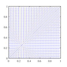
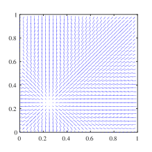
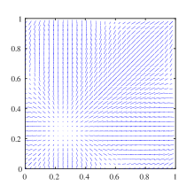
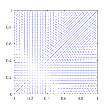
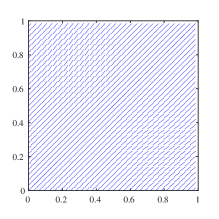
In this experiment, the development of defects are simulated on a period domain. For the domain [0,Lx]ร—[0,Ly][0,L_{x}]\times[0,L_{y}], Lx=Ly=1L_{x}=L_{y}=1, we consider the initial condition

๐0=๐ง0โ€‹๐ง0Tโ€–๐ง0โ€–2โˆ’๐ˆ2,๐ง0=(xโˆ’0.25โ€‹Lx,yโˆ’0.25โ€‹Ly)T.\displaystyle{\bf Q}_{0}=\frac{{\bf n}_{0}{\bf n}_{0}^{T}}{\left\|{\bf n}_{0}\right\|^{2}}-\frac{\bf I}{2},\quad{\bf n}_{0}=(x-0.25L_{x},y-0.25L_{y})^{T}.

Refer to caption

(a) t = 0

Refer to caption

(b) t = 1

Refer to caption

(c) t = 10

Refer to caption

(d) t = 20

Refer to caption

(e) t = 60

Refer to caption

(f) t = 200

Figure 1: Dynamical evolution of director.

Refer to caption

Figure 2: Time evolution of modified energy.

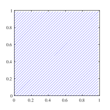
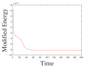
Fig.โ€‰1(a) shows an initial +1+1 type defect at the point (0.25,0.25)(0.25,0.25). In Fig.โ€‰1(b-f), the initial +1+1 type defect gradually escapes. Eventually, the system reaches a steady state. Fig.โ€‰2 shows that the modified energy decreases with time, consistent with our analysis.

5 Conclusion

We carry out a rigorous error analysis for a first-order SAV scheme of 3D hydrodynamic ๐{\bf Q}-tensor model of nematic liquid crystals. The scheme maintains the properties of energy stability and uniqueness of solvability, which are proved in detail. Thus, we derive the rigorous error estimate of order Oโ€‹(ฮดโ€‹t)O(\delta t) in the sense of L2L^{2} norm. Finally, some numerical simulations are given to demonstrate the theoretical analysis.

Acknowledgments

G. Ji is partially supported by the National Natural Science Foundation of China (Grant No. 12471363), X. Li is partially supported by Beijing Normal University grant 312200502508.

References

  • [1] deย Gennesย PG, Prost J, and Pelcovits R. The physics of liquid crystals. Physics Today, 48(5):70โ€“71, 1995.
  • [2] Leslie FM. Some constitutive equations for liquid crystals. Archive for Rational Mechanics and Analysis, 28(4):265โ€“283, 1968.
  • [3] Beris AN and Edwards BJ. Thermodynamics of flowing systems: with internal microstructure. Oxford University Press, 1994.
  • [4] Wang Q, Forest MG, and Zhou R. A hydrodynamic theory for solutions of nonhomogeneous nematic liquid crystalline polymers with density variations. 2002.
  • [5] Zhao J and Wang Q. Semi-discrete energy-stable schemes for a tensor-based hydrodynamic model of nematic liquid crystal flows. Journal of Scientific Computing, 68(3):1241โ€“1266, 2016.
  • [6] Cavaterra C, Rocca E, Wuย H, and Xuย X. Global strong solutions of the full Navier-Stokes and Q-tensor system for nematic liquid crystal flows in two dimensions. SIAM Journal on Mathematical Analysis, 48(2):1368โ€“1399, 2016.
  • [7] Paicu M and Zarnescu A. Energy dissipation and regularity for a coupled Navierโ€“Stokes and Q-tensor system. Archive for Rational Mechanics and Analysis, 203(1):45โ€“67, 2012.
  • [8] Fan J and Ozawa T. Regularity criteria for a coupled Navier-Stokes and Q-tensor system. International Journal of Analysis, 2013:1โ€“5, 2013.
  • [9] Guillรฉn-Gonzรกlez F and รngeles Rodrรguez-Bellidoย M. Weak time regularity and uniqueness for a Q-tensor model. SIAM Journal on Mathematical Analysis, 46(5):3540โ€“3567, 2014.
  • [10] Guillรฉn-Gonzรกlez F and Rodrรญguez-Bellido Mร. Weak solutions for an initialโ€“boundary Q-tensor problem related to liquid crystals. Nonlinear Analysis: Theory, Methods & Applications, 112:84โ€“104, 2015.
  • [11] MacDonald CS, Mackenzie JA, Ramage A, and Newton CJP. Efficient moving mesh methods for Q-tensor models of nematic liquid crystals. SIAM Journal on Scientific Computing, 37(2):B215โ€“B238, 2015.
  • [12] Ramage A and Sonnet AM. Computational fluid dynamics for nematic liquid crystals. BIT Numerical Mathematics, 56(2):573โ€“586, 2016.
  • [13] Cai Y, Shen J, and Xuย X. A stable scheme and its convergence analysis for a 2D dynamic Q-tensor model of nematic liquid crystals. Mathematical Models and Methods in Applied Sciences, 27(08):1459โ€“1488, 2017.
  • [14] Shen J and Yang X. Numerical approximations of Allen-Cahn and Cahn-Hilliard equations. Discrete and Continuous Dynamical Systems, 28(4):1669โ€“1691, 2010.
  • [15] Shen J and Yang X. Decoupled, energy stable schemes for phase-field models of two-phase incompressible flows. SIAM Journal on Numerical Analysis, 53(1):279โ€“296, 2015.
  • [16] Eyre DJ. Unconditionally gradient stable time marching the Cahn-Hilliard equation. MRS Online Proceedings Library, 529(1):39โ€“46, 1998.
  • [17] Zhao J, Yang X, Gong Y, and Wang Q. A novel linear second order unconditionally energy stable scheme for a hydrodynamic Q-tensor model of liquid crystals. Computer Methods in Applied Mechanics and Engineering, 318:803โ€“825, 2017.
  • [18] Yang X. Linear, first and second-order, unconditionally energy stable numerical schemes for the phase field model of homopolymer blends. Journal of Computational Physics, 327:294โ€“316, 2016.
  • [19] Yang X, Zhao J, and Wang Q. Numerical approximations for the molecular beam epitaxial growth model based on the invariant energy quadratization method. Journal of Computational Physics, 333:104โ€“127, 2017.
  • [20] Gudibanda VM, Weber F, and Yue Y. Convergence analysis of a fully discrete energy-stable numerical scheme for the Q-tensor flow of liquid crystals. SIAM Journal on Numerical Analysis, 60(4):2150โ€“2181, 2022.
  • [21] Yue Y. On convergence of an unconditional stable numerical scheme for Q-tensor flow based on invariant quardratization method. 2022.
  • [22] Jiย G. A bdf2 energy-stable scheme for a general tensor-based model of liquid crystals. East Asian Journal on Applied Mathematics, 10(1):57โ€“71, 2020.
  • [23] Shen J, Xuย J, and Yang J. The scalar auxiliary variable (SAV) approach for gradient flows. Journal of Computational Physics, 353:407โ€“416, 2018.
  • [24] Shen J, Xuย J, and Yang J. A new class of efficient and robust energy stable schemes for gradient flows. SIAM Review, 61(3):474โ€“506, 2019.
  • [25] Chen C and Yang X. Fast, provably unconditionally energy stable, and second-order accurate algorithms for the anisotropic Cahnโ€“Hilliard model. Computer Methods in Applied Mechanics and Engineering, 351:35โ€“59, 2019.
  • [26] Sun H and Liu C. On energetic variational approaches in modeling the nematic liquid crystal flows. Discrete and Continuous Dynamical Systems, 23(1/2):455โ€“475, 2008.
  • [27] Wuย H, Xuย X, and Liu C. Asymptotic behavior for a nematic liquid crystal model with different kinematic transport properties. Calculus of Variations and Partial Differential Equations, 45(3-4):319โ€“345, 2012.
  • [28] Wuย H, Xuย X, and Liu C. On the general Ericksenโ€“Leslie system: parodiโ€™s relation, well-posedness and stability. Archive for Rational Mechanics and Analysis, 208(1):59โ€“107, 2013.
  • [29] Huang J and Ding S. Global well-posedness for the dynamical Q-tensor model of liquid crystals. Science China Mathematics, 58(6):1349โ€“1366, 2015.
  • [30] Heย Y and Sun W. Stability and convergence of the crankโ€“nicolson/adamsโ€“bashforth scheme for the time-dependent Navierโ€“Stokes equations. SIAM Journal on Numerical Analysis, 45(2):837โ€“869, 2007.
  • [31] Shen J. Long time stability and convergence for fully discrete nonlinear galerkin methods. Applicable Analysis, 38(4):201โ€“229, 1990.
  • [32] Hou D, Liย X, Qiao Z, and Zheng N. Energy stable and maximum bound principle preserving schemes for the Q-tensor flow of liquid crystals. 2024.