On the Bargmann invariants for quantum imaginarity
Mao-Sheng Li
li.maosheng.math@gmail.comSchool of Mathematics, South China University of Technology, GuangZhou 510640, China
Yi-Xi Tan
School of Mathematics, South China University of Technology, GuangZhou 510640, China
Abstract
The imaginary in quantum theory plays a crucial role in describing quantum coherence and is widely applied in quantum information tasks such as state discrimination, pseudorandomness generation, and quantum metrology. A recent paper by Fernandes et al. [C. Fernandes, R. Wagner, L. Novo, and E. F. Galvão, Phys. Rev. Lett. 133, 190201 (2024)] showed how to use the Bargmann invariant to witness the imaginarity of a set of quantum states. In this work, we delve into the structure of Bargmann invariants and their quantum realization in qubit systems. First, we present a characterization of special sets of Bargmann invariants (also studied by Fernandes et al. for a set of four states) for a general set of
quantum states. Then, we study the properties of the relevant Bargmann invariant set
and its quantum realization in qubit systems. Our results provide new insights into the structure of Bargmann invariants, contributing to the advancement of quantum information techniques, particularly within qubit systems.
I Introduction
Quantum theory’s reliance on complex numbers is well-established [1, 2]. Fundamental concepts in quantum theory, such as quantum states, measurements, and evolutions, are intrinsically tied to complex numbers. The quantification of the imaginary parts of quantum states, referred to as quantum imaginarity, has emerged as a valuable resource, driving significant advancements in quantum information science [3, 4, 5, 6, 7, 8]. Although some works have explored the possibility of formulating quantum theory within a real vector space, proposing frameworks for quantum computing and information processing based on real-number operations [9, 10, 11, 12], both theoretical and experimental results [13, 14, 15, 16, 17, 18] have established the necessity of quantum imaginarity for accurately modeling certain quantum phenomena. These findings highlight the fundamental and indispensable role of quantum imaginarity in the precise description and manipulation of quantum systems. As a resource, quantum imaginarity has found applications in a wide range of quantum information tasks, including state discrimination [19], pseudorandomness generation [20], and quantum metrology [21].
Since the seminal works [13, 14, 22], numerous studies have focused on quantifying quantum imaginarity or the resource theory of quantum imaginarity, employing tools such as the -norm, trace norm, and various entropies, while also exploring its diverse applications [16, 23, 24, 25, 26, 27, 28, 17, 29, 30, 31, 32, 33, 26, 34, 35, 36]. Similar to quantum coherence, the imaginarity of a state depends on the choice of the computational basis. By studying the imaginarity of a set of quantum states, one can achieve a basis-independent characterization of quantum imaginarity [37]. More recently, in Ref. [38], the authors explored how to witness quantum imaginarity by examining unitary-invariants, specifically the Bargmann invariants [39], in sets of quantum states. They provided a comprehensive characterization of the Bargmann invariants for three pure states (i.e., ) and a partial characterization for four states, focusing on a subset of the full set of Bargmann invariants for four pure states. Most notably, they demonstrated that the imaginarity of four-state sets can be effectively witnessed through pairwise overlaps, a result that, intriguingly, does not extend to sets of three states. This pivotal finding significantly advances our understanding of quantum imaginarity but raises several intriguing questions, such as how to characterize the Bargmann invariants for sets with more than four states and how to realize these invariants in a qubit system. In this work, we provide a deeper exploration of these questions and offer partial solutions to these challenges.
The general content and structure of this paper are as follows:
In Sec. II, we introduce the basic concepts of basis-independent imaginary sets, Bargmann invariants, and the relationship between them.
In Sec. III, we present a complete characterization for a subset, , of Bargmann invariants for states and discuss some properties of the total Bargmann invariant set .
In Sec. IV, we demonstrate that all Bargmann invariants in can be realized using qubits.
Finally, we conclude and make a discussion of our findings in Sec. V.
II Preliminaries
Throughout this paper, denote the set of all integers, real numbers, and complex numbers, respectively. Let be a quantum system of dimension , denote the set of all density matrices (self-adjoint, positive semidefinite matrices with trace 1), and represent the set of pure states in the system . For simplicity, we will denote as the density matrix of the pure state , i.e., .
Given an ordered set of quantum states , we are interested in determining whether there exists a basis such that all elements of have real entries. Equivalently, we seek to determine whether there exists a unitary such that for all , the transformed states lie in . If no such basis exists, we call the set a basis-independent imaginary set. The Bargmann invariants, defined as the quantity , are clearly basis-independent and are used to characterize such a set. In fact, the imaginarity of the value implies the basis-independent imaginarity of the set .
Let denote the set of all Bargmann invariants of length states in , i.e.,
We are, in fact, more interested in considering pure states. Therefore, we define
In this case, we have the identity
This leads to the following ascending chain of sets:
and we define
Let . We define to be unitary equivalent to (denoted ) if there exists a unitary matrix such that
The equivalence class of elements in under unitary transformations can be characterized by their Gram matrices. Specifically, we define as the matrix whose -th entry is .
Under this definition, two tuples are unitarily equivalent if and only if their associated Gram matrices satisfy .
The following lemma provides a characterization of the conditions under which a Hermitian matrix can arise as a Gram matrix corresponding to a set of pure states.
Let be any candidate Hermitian matrix. Then, is positive semidefinite with principal diagonal entries if and only if there exists some (which depends on ) and some such that .
Let denote the set of all Hermitian matrices that are positive semidefinite and have for all . Based on this lemma, one can easily conclude that
Throughout this paper, for , we will use the notation to denote the number
Under this notation, the expression is equivalent to
A matrix is circulant if it has the form
(1)
where .
We denote the set of all circulant matrices as . It follows that
Let , i.e., is the special circulant matrix given by
Then, the circulant matrix defined in Eq. (1) can be written as
Thus, the Bargmann invariant set is
(2)
III Properties of Bargmann invariant sets
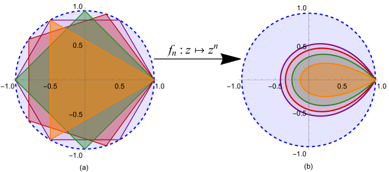
Figure 1: The set . (a). The regions of (b). Sets of quantum-realizable Bargmann invariants of
Note that , , and , as revealed in Ref. [38]. It was conjectured that the set , where the boundary of is characterized by the following points:
Although has been known, it has not been established whether . To address this, we first need to characterize the set . For a circulant matrix to be positive semidefinite, it must take the following form (i.e., ):
The eigenvalues of the above matrix are:
where . Let . To ensure that these eigenvalues are nonnegative, the following conditions must hold:
(3)
Denote the triangle defined by these inequalities as (see Fig. 1). We then find that
It is easy to check that the set is exactly . Since is characterized by the latter set [38], we conclude that .
Next, we confirm this result using a different method. Since we always have , we need only check the reverse inclusion .
For each , there exists a matrix such that
Without loss of generality, we assume that
Thus, . Since , we have and
(4)
Let
The matrix belongs to if and only if and
(5)
Clearly, the first condition holds.
For the second condition, we consider
The last inequality holds by applying the well-known inequality
Thus, we conclude that
Hence, . Since where , we have
Therefore, . To conclude, we have .
Thus, the Bargmann invariant set is exactly characterized by
We have thus reproduced Theorem 1 of Ref. [38] by an alternative method.
Now, we seek to characterize the set for . Consider a positive semidefinite circulant matrix, which must take the following form:
where and . The eigenvalues of are:
From these conditions, we deduce that:
which describes a square (see Fig. 1) centered at with as one of its vertices. Therefore, we find that:
This result regarding the characterization of and can be generalized to for higher .
Let denote the region enclosed by a regular -sided polygon centered at the origin with one vertex at in the complex plane. Define the map by
Next, let
By Eq. (2), we have . Thus, we characterize as the image of the regular polygon under , as follows.
Theorem 1.
For each , the Bargmann invariant set is exactly the image of the set under the map , i.e.,
Sketch of the proof: To prove this, we need to show that . We prove this equality in four steps, which are detailed in Appendix A.
Step 1: Show that .
Step 2: If , then (where ).
Step 3: Prove that is a convex set.
Step 4: Show that for each , the point must below the line
which corresponds to a line passing through the points and .
Steps 1 and 2 establish that , while Steps 2 and 4 imply that . Therefore, we conclude that . ∎
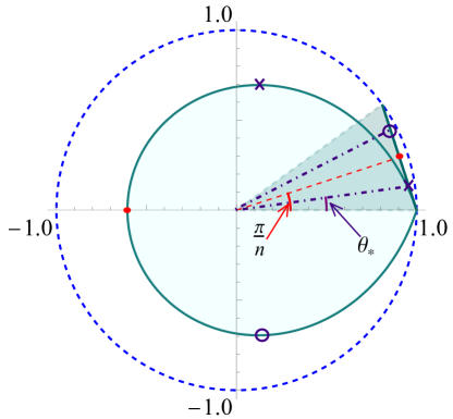
In fact, the image is an -fold cover of . We can decompose the polygon into triangles, , such that for each . For instance, in Fig. 2, the triangle is plotted in green, and the image of the green edge under the map is exactly the green curve , which represents the boundary of .
Figure 2: Three special points on the boundary of the Bargmann invariant set are considered: the point labeled by ‘’ or ‘’ corresponds to the maximal imaginarity , while the red bullet ‘’ corresponds to the minimal real number in . Additionally, we indicate how these three points arise from the map , which is applied to the edge (the line connecting and ) of .
We can also express the boundary curve of in polar coordinates. Let and . Then there exists such that
where .
The radius is given by
(6)
The phase satisfies
(7)
From this equation, we deduce that
Substituting this into Eq. (7), we obtain the relationship between and .
For a complex number , define
which measures the imaginary part of . It is interesting to find the maximal imaginarity contained in . We observe that
where (see Fig. 2 for an intuitive representation of the value of ).
In fact, we only need to consider for . Note that
Writing in the form , and referring to the geometry shown in Fig. 2, we have the relation
Therefore,
It is natural to define the function
We then find that
Setting , we obtain , which corresponds to an optimal value (see the points label with in Fig. 2). Moreover, the relationship between and is given by
One can also determine the optimal parameter , which may be useful for experiments.
We are primarily interested in understanding the nature of the set . First, by definition, we have the following inclusion:
Naturally, one might ask whether the reverse inclusion holds, i.e., whether we have
For each , we can associate it with a circulant matrix , where the coefficients are given by
with and , where and . It is important to note that the Bargmann invariants corresponding to and are equal, i.e.,
For the case when , we deduced that the positive semidefiniteness of follows from the positive semidefiniteness of . This leads us to the conjecture that the positive semidefiniteness of implies the positive semidefiniteness of (which may depend on ) for general . If this conjecture holds, we would then have .
For the time being, we have not been able to prove this strong result. Instead, we present some properties of the set in the following propositions (see Proposition 1, 2, and 3).
Let us first recall the definition of the Hadamard product of two matrices. Given two matrices and in , the Hadamard product is also an matrix whose -th entry is .
Proposition 1.
If , then their Hadamard product . As a consequence, is closed under multiplication. Specifically, if , then .
Proof.
A matrix if and only if there exists a set of quantum states such that . Suppose that and , where and . Then we have the tensor product of two sets of quantum states:
It can be checked that
For the latter statement, if , then there exist and such that
By the previous argument, the Hadamard product , and thus the product
This completes the proof.
∎
Although we cannot prove the inclusion at this time, we can bound by a superset.
Proposition 2.
Let be an integer. Then we have
Proof.
For any , there exists a Gram matrix such that . For each , we define
It can be verified that the product
is not only in , but is also a circulant matrix. Specifically, if we define
where , for , then
By Proposition 1, , and therefore . Since , it follows that . Thus, we conclude that
∎
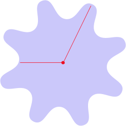
Figure 3: The figure is a diagram of a set with star-shaped. Note that a set with star-shaped is not necessarily a convex set.
Proposition 3.
Let be an integer. Then the set is star-shaped with the center at (see Fig. 3 for an intuitive representation of a star-shaped set). That is, if , then all points lying between and are also in .
Proof.
For , we know that , which is clearly a star-shaped set centered at . Thus, we only need to consider the case . Clearly, .
For each , there exists a set of quantum states such that
We need to show that for each , the point .
Since , we have for all . Let , where and . If , we replace by . Therefore, we can always assume that , where is a positive real number.
Since , there always exists a state orthogonal to . Let this state be denoted as . By choosing an appropriate global phase for , we can also assume that is a real number, which we denote by . Replacing the second state of by , we obtain a new set of states .
The states and are linearly independent. Otherwise, if , we would have . For each , we define a pure state
where is the norm of the vector , which is nonzero due to the linear independence of and . Note that is a family of pure states that connect and .
Now, consider the set of states
The corresponding Bargmann invariant arising from is
Set
Since , we have
Substituting the expression for into the definition of , we get
This simplifies to
Therefore, is a continuous real-valued function on with and . Since for all , by the mean value theorem for continuous functions, there exists some such that
For such , we have
This shows that for all , completing the proof.
∎
IV Quantum realization of Bargmann invariants in qubit system
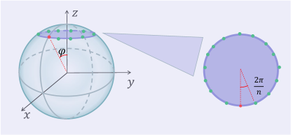
In the remark for the proof of Theorem 1, we pointed out that each point on the boundary of has a quantum realization in a qubit system, i.e., . Here, we provide a more constructive proof of this statement and a stronger result.
Figure 4: A visualization of the -tuple states , as given by Eq. (8), in the context of the Bloch sphere.
Theorem 2.
For each , any element in the Bargmann invariant set can be realized in a qubit system. That is,
Proof.
First, observe that represents the region whose boundary is characterized by the curve:
where . We claim that
. , set as an -tuple of single-qubit states, where (see Fig. 4)
(8)
for . The -order Bargmann invariant of is given by
Let , so . Therefore, for each ,
Thus, we have .
By Proposition 3, contains the set of all points connecting 0 to some point on . Therefore, we conclude that
∎
If the value contains a nontrivial imaginary part, one can conclude the imaginarity of the -tuple set . It is of interest to consider whether there exist any real numbers of the form that could only arise from some quantum state set with imaginarity. This motivates us to define
Theorem 3.
For each , we have the following relation:
As a consequence, for each -order real Bargmann invariant , there exists a realization of using real states alone.
Proof.
First, we show . For any , there exists such that
Since each , it can be written as
Thus,
This simplifies to
To find the maximal and minimal values of the function
we compute the partial derivatives, leading to the equation . Therefore, . That is, (here, if and only if ). Set , then we have and There is only one such that . So we have
So for some And for some Then
where the exponential . For the case , i.e., , we should have
which implies and the corresponding For all other ,
we have Hence
On the other hand, the value can be achieved by setting and . This shows that . Therefore, we conclude that
∎
At present, it is not known whether . If this equality holds, the real Bargmann invariant would provide no additional information. However, if the equality does not hold, there would exist some real Bargmann invariant from which we could also deduce the imaginarity of the corresponding set.
Note that In fact, for each , there exists such that
And we set , then
So . It is highly challenging to determine the exact form of the set . Therefore, it is of particular interest to investigate the limit of these sets, which motivates us to define
We will show that the limit set can be fully described by The set
represents the open unit disk in the complex plane along with the point 1.
Theorem 4.
Fix an integer For each , the value can be realized in for some . That is, there exists some and () such that Moreover, we have the identity
Proof.
First, we show that Fix . If clearly, Otherwise, with As , there exists some such that Let . By the geometirc intuition of Fig. 2, we have . Therefore,
As , we have
Let . There exists such that
Clearly, the modulus of satisfies
. The equality holds if and only if whose corresponding is exactly . For all other cases, hence Therefore,
∎
V Conclusions and Discussion
We have studied the Bargmann invariants, which are pivotal in detecting the quantum imaginarity of sets of quantum states. We have provided complete characterizations of the Bargmann invariant sets and for all . For (), we have examined several of its properties, including multiplicative closure, star-shapedness, and have derived both upper and lower bounds. Furthermore, we have shown that the Bargmann invariants in can be realized within a qubit system, and have determined the maximum imaginarity for this set. Additionally, we have established that the real Bargmann invariants in can be realized by real qubit states. Finally, we have completely characterized the set of all Bargmann invariants, denoted by .
Our work advances the understanding of Bargmann invariants, emphasizing their critical role in detecting quantum imaginarity in quantum states. Looking ahead, the full characterization of the Bargmann invariant sets for remains an open challenge. Furthermore, the question of whether there exist real Bargmann invariants that cannot be realized by real states continues to be an intriguing avenue for future research.
Acknowledgements.
This work was supported by National Natural Science Foundation of China under Grants No. 12371458, the Guangdong Basic and Applied Basic Research Foundation under Grants Nos. 2023A1515012074, 2024A1515010380 and the Science and Technology Planning Project of Guangzhou under Grants No. 2023A04J1296.
Before the proof, we make a remark. First, we only consider as a Hermitian matrix which is equivalent to for all . As are all the eigenvalues of the matrix , so the eigenvalues of the matrix are exactly given by To simplify the notation, we will always assume and as a column vector. Let denote the set of all -tuples with conditions and for . Let denote the dimensional Fourier transformation, i.e.,
If , then which implies all eigenvalues of are real. Therefore, the positive semidefinite of is equivalent to for every , i.e.,
Then the set can be expressed as
(9)
Now we start to prove the four steps.
Step 1: Show that .
Let with for all . Clearly, and So .
Step 2: If , then (where ).
As , there exists a whose second entry is exactly such that . That is,
(10)
Set . Clearly, , for and . Hence . Moreover, we can check that In fact,
Therefore, the second entry of , i.e., , belongs to .
Step 3: The set is a convex set.
Given and .
There exist such that and Set . It is easy to verify that and
Hence,
Step 4: For each , the point must below the line which passing through points and .
Given such that , i.e., Eq.(10) holds. In the following, we need to show
Equivalentlly,
(11)
Note that equals to the real part of Set where and As , Eq. (11) can be rewritten as
(12)
As , for each , i.e., every entry is nonnegative, we have
(13)
Theofore, to prove Eq. (12), it is sufficient to find some such that
In fact, to ensure the latter condition, must be . So we only need to show As
we have
Hence, or , and for , This proves
∎
Remark: If lies on the boundary of and such that , we claim that the rank of corresponding Gram matrix does not greater than 2. Without loss of generality, we assume is on the line . Let be the vectors as in the proof of Theorem 1 and be eigenvalues of .
Then we have
At the end of the above proof, we point out that for or , and for , So we have . From these conditions and , we must have Therefore, So such Gram matrix can be realized in two dimensional system.
References
Griffiths [2004]D. J. Griffiths, Introduction to
Quantum Mechanics, 2nd ed. (Cambridge University Press, 2004).
Gibbons and Pohle [1993]G. Gibbons and H.-J. Pohle, Complex numbers, quantum
mechanics and the beginning of time, Nuclear Physics B 410, 117 (1993).
Streltsov et al. [2017]A. Streltsov, G. Adesso, and M. B. Plenio, Colloquium: Quantum coherence as a
resource, Rev. Mod. Phys. 89, 041003 (2017).
Dressel and Jordan [2012]J. Dressel and A. N. Jordan, Significance of the
imaginary part of the weak value, Phys. Rev. A 85, 10.1103/physreva.85.012107
(2012).
Kunjwal et al. [2019]R. Kunjwal, M. Lostaglio, and M. F. Pusey, Anomalous weak values and
contextuality: Robustness, tightness, and imaginary parts, Phys. Rev. A 100, 042116 (2019).
Aleksandrova et al. [2013]A. Aleksandrova, V. Borish, and W. K. Wootters, Real-vector-space
quantum theory with a universal quantum bit, Phys. Rev. A 87, 052106 (2013).
McKague et al. [2009]M. McKague, M. Mosca, and N. Gisin, Simulating Quantum Systems Using Real
Hilbert Spaces, Phys. Rev. Lett. 102, 020505 (2009).
Nielsen and Chuang [2010]M. A. Nielsen and I. L. Chuang, Quantum Computation and
Quantum Information: 10th Anniversary Edition (Cambridge University Press, 2010).
Renou et al. [2021]M.-O. Renou, D. Trillo,
M. Weilenmann, T. P. Le, A. Tavakoli, N. Gisin, A. Acin, and M. Navascues, Quantum theory based on real numbers can be experimentally falsified, Nature 600, 625 (2021).
Wu et al. [2021a]K.-D. Wu, T. V. Kondra,
S. Rana, C. M. Scandolo, G.-Y. Xiang, C.-F. Li, G.-C. Guo, and A. Streltsov, Operational resource theory of imaginarity, Phys. Rev. Lett. 126, 090401 (2021a).
Chen et al. [2022a]M.-C. Chen, C. Wang, F.-M. Liu, J.-W. Wang, C. Ying, Z.-X. Shang, Y. Wu, M. Gong, H. Deng, F.-T. Liang, Q. Zhang, C.-Z. Peng, X. Zhu, A. Cabello, C.-Y. Lu, and J.-W. Pan, Ruling out real-valued standard
formalism of quantum theory, Phys. Rev. Lett. 128, 040403 (2022a).
Wu et al. [2024]K.-D. Wu, T. V. Kondra,
C. M. Scandolo, S. Rana, G.-Y. Xiang, C.-F. Li, G.-C. Guo, and A. Streltsov, Resource theory of imaginarity in distributed scenarios, Communications Physics 7, 1 (2024).
Yao et al. [2024]J. Yao, H. Chen, Y.-L. Mao, Z.-D. Li, and J. Fan, Proposals for ruling out real quantum theories in an
entanglement-swapping quantum network with causally independent sources, Phys. Rev. A 109, 012211 (2024).
Zoratti et al. [2021]F. Zoratti, N. Dalla Pozza, M. Fanizza, and V. Giovannetti, Agnostic dolinar
receiver for coherent-state classification, Phys. Rev. A 104, 042606 (2021).
de la Torre et al. [2015]G. de la Torre, M. J. Hoban, C. Dhara,
G. Prettico, and A. Acín, Maximally nonlocal theories cannot be maximally
random, Phys. Rev. Lett. 114, 160502 (2015).
Wu et al. [2021b]K.-D. Wu, T. V. Kondra,
S. Rana, C. M. Scandolo, G.-Y. Xiang, C.-F. Li, G.-C. Guo, and A. Streltsov, Resource theory of imaginarity: Quantification and state conversion, Phys. Rev. A 103, 032401 (2021b).
Li et al. [2022]N. Li, S. Luo, and Y. Sun, Brukner-zeilinger invariant information in the
presence of conjugate symmetry, Phys. Rev. A 106, 032404 (2022).
Chen et al. [2024]B. Chen, X. Huang, and S.-M. Fei, On complementarity and distribution of imaginarity
in finite dimensions, Results in Physics 60, 107671 (2024).
Oszmaniec et al. [2024]M. Oszmaniec, D. J. Brod, and E. F. Galvão, Measuring relational
information between quantum states, and applications, New J. Phys. 26, 013053 (2024).
Fernandes et al. [2024]C. Fernandes, R. Wagner,
L. Novo, and E. F. Galvão, Unitary-invariant witnesses of quantum
imaginarity, Phys. Rev. Lett. 133, 190201 (2024).
Simon and Mukunda [1993]R. Simon and N. Mukunda, Bargmann invariant and
the geometry of the Güoy effect, Phys. Rev. Lett. 70, 880 (1993).