GLL: A Differentiable Graph Learning Layer for Neural Networks
Abstract
Standard deep learning architectures used for classification generate label predictions with a projection head and softmax activation function. Although successful, these methods fail to leverage the relational information between samples in the batch for generating label predictions. In recent works, graph-based learning techniques, namely Laplace learning (Zhu et al. (2003)) or label propagation, have been heuristically combined with neural networks for both supervised and semi-supervised learning (SSL) tasks. However, prior works approximate the gradient of the loss function with respect to the graph learning algorithm or decouple the processes; end-to-end integration with neural networks is not achieved. In this work, we derive backpropagation equations, via the adjoint method, for inclusion of a general family of graph learning layers into a neural network. This allows us to precisely integrate graph Laplacian-based label propagation into a neural network layer, replacing a projection head and softmax activation function for classification tasks. Using this new framework, our experimental results demonstrate smooth label transitions across data, improved robustness to adversarial attacks, improved generalization, and improved training dynamics compared to the standard softmax-based approach111Our code is available at https://github.com/jwcalder/GraphLearningLayer.
Keywords: Graph learning, deep learning, Laplace learning, label propagation, adversarial robustness
1 Introduction
Graph-based learning is a powerful class of transductive machine learning techniques that leverage the topology of a similarity graph constructed on the data for tasks such as semi-supervised learning, data visualization, and dimension reduction. Beginning with the seminal work by Zhu et al. (2003) on semi-supervised learning, graph-based learning techniques have since proliferated (Belkin and Niyogi, 2004; Belkin et al., 2004; Bengio et al., 2006; Zhou and Belkin, 2011; Wang et al., 2013; Ham et al., 2005; Lee et al., 2013; Calder et al., 2020; Calder and Slepcev, 2020; Shi et al., 2017) and found applications in many problem areas. Graphs may be intrinsically present in a data set, such as in network science problems, where relational information is present in links between servers in a network, or between users on social media platforms, or the data points themselves may be graphs (e.g., molecules in drug discovery). Another important graph representation is the similarity graph, which encodes the notion of similarity between pairs of data points. In this paper, we focus on graph-based learning using similarity graphs; that is, we do not assume the graph is given as part of the metadata in the problem. Thus, our work is orthogonal and complementary to much of the graph neural network literature, where the graph is a priori fixed.
Similarity graphs and corresponding graph techniques have been extensively studied theoretically using variational analysis, random walks, harmonic functions, and partial differential equations (see e.g., Calder (2019); Calder and García Trillos (2022); Calder and Slepcev (2020); Calder (2018); Slepcev and Thorpe (2019); Dunlop et al. (2020); García Trillos et al. (2020); Hein et al. (2007, 2005); Calder and Ettehad (2022); Calder et al. (2023)). Graph learning also contrasts with modern deep learning approaches in that it is a data-dependent model without any trainable parameters. Previous works (Chapman et al., 2023; Chen et al., 2023a, b) show that graph learning outperforms many popular classifiers like support vector machine (Cortes and Vapnik (1995)), random forest (Ho (1995)), and neural networks on classification tasks, especially at very low label rates.
Recently, many works have focused on combining graph-based learning with deep learning. In such works, unsupervised or semi-supervised neural networks learn an embedding of the data into a feature space and use the similarity between features to construction the graph. Examples of such deep learning techniques include variational autoencoders (VAEs) (Kingma and Welling (2013); Calder et al. (2020); Calder and Ettehad (2022)), convolutional neural networks (CNNs) (LeCun et al. (1989); Enwright et al. (2023)), convolutional VAEs (Pu et al. (2016); Miller et al. (2022); Chapman et al. (2023)), and contrastive learning (Chen et al. (2020a); Brown et al. (2023b, a)). Some works have used graph learning to generate pseudolabels to train a deep neural network in low label rate settings (Sellars et al. (2021); Iscen et al. (2019)). Another recent approach replaces the softmax activation with graph learning to improve generalization and adversarial robustness (Wang and Osher (2021)); however, the gradients of the loss with respect to the graph learning classifier are only approximated by an equivalently-sized linear classifier.
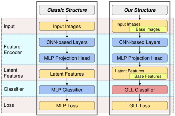
A significant gap in the literature exists, as no work fully integrates graph learning into the gradient-based learning framework of neural networks. In this paper, we leverage the adjoint graph Laplace equation to derive the exact backpropagation gradients for a general family of graph learning methods, and show how to implement them efficiently. This significantly expands upon the previous work by Enwright et al. (2023), where the backpropagation equations were only derived for Laplace learning on a fully connected graph. The backpropagation equations allow us to design a neural network layer that replaces the standard projection head and softmax classifier with a graph learning classifier (see Figure 1). We call this novel layer the Graph Learning Layer (GLL). GLL can be combined with any neural network architecture and enables end-to-end training in a gradient-based optimization framework. Through a variety of experiments, we show that GLL learns the intrinsic geometry of data, improves the training dynamics and test accuracy of both shallow and deep networks, and is significantly more robust to adversarial attacks compared to a projection head and softmax classifier.
1.1 Related Work
Graph-based semi-supervised learning (SSL) methods construct a graph that allows inferences of unlabeled nodes using labeled nodes and the graph topology. The seminal work of Laplace learning (Zhu et al. (2003)), also known as label propagation, led to a proliferation of related techniques (Belkin and Niyogi, 2004; Belkin et al., 2004; Bengio et al., 2006; Zhou and Belkin, 2011; Wang et al., 2013; Ham et al., 2005; Lee et al., 2013; Garcia-Cardona et al., 2014; Calder and Slepcev, 2020; Shi et al., 2017). Laplace learning computes a graph harmonic function to extend the given labels to the remainder of the graph—essentially finding the smoothest function that agrees with the given labels. When the label rate is low (i.e., close to one label per class), Laplace learning degenerates and suffers from a “spiking” phenomenon around labeled points, while predictions are roughly constant (Calder et al. (2020); El Alaoui et al. (2016); Nadler et al. (2009)). Several methods have been proposed for these very low label rate regimes including reweighted Laplace learning (Shi et al. (2017); Calder and Slepcev (2020); Miller and Calder (2023)), -Laplace methods (Zhou and Belkin (2011); El Alaoui et al. (2016); Flores et al. (2022); Slepcev and Thorpe (2019)), and Poisson learning (Calder et al. (2020)). Analysis of the degeneracy of Laplace learning from a random walk and variational perspective can be found in (Calder et al. (2020, 2023)). Some recent work has also focused on graph total variation problems using graph cuts (Bertozzi and Flenner (2016); Merkurjev et al. (2017, 2018)).
Another related, but distinct, area of work in machine learning on graphs is graph neural networks, or GNNs (Kipf and Welling, 2016; Defferrard et al., 2016; Wu et al., 2020). The GNN literature considers how to incorporate a priori graph information relevant to the task, such as co-authorship in a citation graph, within a neural network architecture for various learning tasks, such as learning node embeddings or semi-supervised learning. These works are quite different. In particular, we do not assume the data has a graph structure. Moreover, GNNs contain trainable weight matrices, while graph-based learning methods have no trainable parameters. There are some works, such as graph attention networks (Velicković et al., 2017), which learn how to assign weights to a graph, but the graph adjacency structure is still fixed a priori through the masking in the attention mechanism.
Previous work by Agrawal et al. (2019) studied backpropagation techniques for the differentiation of convex optimization problems. Our paper extends this work to nonlinear equations on graphs involving graph Laplacians.
Deep learning methods have increasingly leveraged graph-based approaches or drawn inspiration from them. Two recent works propagate labels on a graph to generate pseudolabels in a semi-supervised setting (Iscen et al. (2019); Sellars et al. (2021)). However, the label propagation process is disconnected from the neural network and not directly integrated into the backpropagation or learning process. Contrastive learning (CL) uses pair-wise similarity, akin to a complete similarity graph, to facilitate the learning process (Chen et al. (2020b, a); Khosla et al. (2020); Wang et al. (2023)). Wang and Osher (2021) utilize graph learning as a classifier within a neural network, but they approximate the backpropagation gradients instead of computing them exactly.
1.2 Our Contributions
The most significant difference between our work and any of the preceding works is the derivation and implementation of the exact backpropagation equations through the graph learning layer, including the similarity graph construction and the graph-based classifier. We also give a sparse, efficient implementation of these equations. This is a significant extension of Enwright et al. (2023), where the authors derive the backpropagation gradients for Laplace learning in the special case of a fully connected graph. In this work, we derive the gradients for any -nearest neighbors-type graph construction and any nonlinear elliptic graph learning equation. In addition, we conduct detailed experiments on a variety of benchmark datasets and neural network architectures. Our analysis includes visualizing clustering effects in the latent space under different GLL hyperparameters, demonstrating improved training dynamics and generalization, and showcasing improved robustness to adversarial attacks. In many experiments, GLL outperforms the standard projection head and softmax-based classifier.
The remainder of the paper is organized as follows. Section 2 details the necessary background on Laplace Learning, the seminal graph-based learning algorithm. Section 3 describes our novel mathematical contributions powering our novel GLL. Namely, we derive the gradient of the loss with respect to the similarity graph weight matrix and the associated -Nearest Neighbor graph construction, which allows us to integrate graph learning into a neural network training context. We also demonstrate the effect this novel GLL has on the learned neural network embeddings. Section 4 contains illustrative experimental results showcasing the viability of the GLL on classification tasks with benchmark datasets, demonstrating strong classification accuracy as well as improved generalization and robustness to adversarial attacks compared to the softmax classifier.
2 Background
In this section, we give some background on construction similarity graphs, calculus on graphs, and graph learning using various types of graph Laplace equations.
2.1 Similarity Graph Construction
In this paper, we use an approximate -nearest neighbor search using the Annoy python package222https://github.com/spotify/annoy. The weights are computed between the feature vectors of neighboring nodes and using the radial basis function
| (1) |
The bandwidth parameter is the distance from to its th nearest neighbor, which allows the weights to self-tune appropriately to areas of density and sparsity. If desired for applications, may be set to a constant value for all . Because the k-nearest neighbor search is not necessarily symmetric, we symmetrize the weight matrix by replacing with .
2.2 Calculus on graphs
Let be the vertex set of a graph with vertices and nonnegative edge weights , for . Let denote the weight matrix for the graph. We always assume the weight matrix is symmetric, so .
We let denote the Hilbert space of functions , equipped with the inner product
| (2) |
and norm . For we also define -norm
| (3) |
The degree is a function with defined by
We let denote the space of functions . A vector field on the graph is a function that is skew symmetric, so . We use bold face for vector fields to distinguish from functions on the graph. The gradient of defined by
| (4) |
is an example of a vector field over the graph. For we define an inner product
| (5) |
together with a norm .
The graph divergence is as an operator taking vector fields to functions in , and is defined as the adjoint of the gradient. Here, we define the divergence for any function ; that is, it may not be a vector field. Hence, for , the graph divergence is defined so that the identity
| (6) |
holds for all . A straightforward computation shows that
| (7) |
If is a vector field, then this can be simplified to
| (8) |
The gradient is an operator , and the divergence is an operator . The graph Laplacian is the composition of these two operators , which can be expressed as
| (9) |
By the definition we have
for any . In particular, we have
which is the Dirichlet energy on the graph. For a connected graph with , the kernel of the graph Laplacian is -dimensional and spanned by the vector of all ones. In general, the multiplicity of the eigenvalue indicates the number of connected components in the graph (Von Luxburg (2007)).
2.3 Classical Graph-based Learning
Let be a set of -dimensional feature vectors. Let be the set of labeled indices that identifies which feature vectors have labels (for a -class classification problem). The task of semi-supervised learning is to infer the labels on the unlabeled index set . The labels are represented by one-hot vectors; that is, the vector of all zeros, except a 1 in the entry. We use the geometric structure of a similarity graph constructed on to make predictions. Using a symmetric similarity function , we construct the similarity graph’s weight matrix , where or is the edge weight between and ( denotes generic elements ). The weight matrix is symmetric and the edge weights correspond to similarity between nodes, with larger values indicating higher similarity. Because pairwise similarities and dense matrix operations are expensive to compute, is typically approximated using a sparse or low rank representation. Here we use a -nearest neighbors search on with so that is sparse (see Section 2.1).
Laplace learning (Zhu et al. (2003)), also called label propagation, is a seminal method in graph-based learning. The labels are inferred by solving the graph Laplace equation
| (10) |
where encodes the labeled data through their one hot vector representations. The solution is a function where the components of can be interpreted as the probability that belongs to each class. The label prediction is the class with the highest probability. Equation (10) is a system of linear equations, one for each class, which are all completely independent of each other. Thus, this formulation of Laplace learning is equivalent to applying the one-vs-rest method for converting a binary classifier to the multiclass setting.
Laplace learning also has a variational interpretation as the solution to the problem
| (11) |
subject to the condition that on the labeled set . The necessary condition satisfied by any minimizer of (11) is exactly the Laplace equation (10). Furthermore, as long as the graph is connected333In fact, a weaker condition that the graph is connected to the labeled data is sufficient, which is equivalent to asking that every connected component of the graph has at least one labeled data point. the solution of (10) exists and is unique, as is the minimizer of (11) (see Calder (2018)).
There are variants of Laplace learning that employ soft constraints on the agreement with given labels, which can be useful when there is noise or corruption of the labels, typical in many real world settings. Fixing a parameter , the soft-constrained Laplace learning problem minimizes
| (12) |
where tunes the tradeoff between label fidelity and label smoothness. Provided the graph is connected, the unique minimizer of (12) is the solution of the graph Laplace equation
| (13) |
where if and if . We recover Laplace learning (10) in the limit as .
The graph Laplace equations (10) and (13) are positive definite symmetric linear equations, and can be solved with any number of direct or indirect techniques. When the size of the problem is small, a direct matrix inversion may be used. For larger problems, especially for large sparse systems, an iterative method like the preconditioned conjugate gradient method is preferred.
There are also a variety of graph-based learning techniques that do not require labeled information, such as the Ginzburg-Landau formulation (Garcia-Cardona et al., 2014)
| (14) |
where is a many-well potential, with wells located at the one hot label vectors. For binary classification, the wells may be positioned at and . The MBO methods pioneered by Merkurjev et al. (2013); Garcia-Cardona et al. (2014) are effective approximations of the Ginzburg-Landau energy (14) when . This method was first developed in a semi-supervised setting but also used for modularity optimization Boyd et al. (2018) and a piecewise constant Mumford-Shah model in an unsupervised setting Hu et al. (2015).
2.4 Diagonal Perturbation
A modification to Laplace learning (Section 2.3) is to add a type of Tikhonov regularization in the energy (see e.g. Miller and Calder (2023)), leading to the minimization problem
| (15) |
subject to the condition that on the labeled set . Tikhonov regularization can also be added to the soft constrained Laplace learning (12). The minimizer of (15) is the solution of the graph Laplace equation (10) except that the graph Laplacian is replaced by the diagonal perturbed Laplacian (likewise for the soft constrained problem (13)).
This regularization term increases the convergence speed of iterative algorithm by improving the condition number of the graph Laplacian. Moreover, it induces exponential decay away from labeled data points. This inhibits label propagation and weakens predictions further from labeled data in the latent space, which can limit overconfident predictions. In Section 4.1, we show that employing this regularization in GLL causes denser clustering of similar samples in the latent space learned by the neural network, which may be desireable for classification tasks.
2.5 -Laplace learning
There are also graph-learning methods based on the nonlinear graph -Laplacian (Zhou and Belkin (2011); El Alaoui et al. (2016); Flores et al. (2022); Slepcev and Thorpe (2019); Calder (2018)). One such example is the variational -Laplacian, which stems from solving the optimization problem
| (16) |
subject to on . Taking values of was proposed in (El Alaoui et al., 2016) as a method for improving Laplace learning in the setting of very few labeled data points, and analysis of the -Laplacian was carried out in Slepcev and Thorpe (2019); Calder (2018). The minimizer of the -variational problem (16) solves the graph -Laplace equation
| (17) |
Another form of the -Laplacian—the game theoretic -Laplacian—was proposed and studied in (Calder, 2018; Calder and Drenska, 2024).
2.6 Poisson learning
Another recently proposed approach for low label rate graph-based semi-supervised learning is Poisson learning (Calder et al., 2020). Instead of solving the graph Laplace equation (10), Poisson learning solves the graph Poisson equation
where , is the number of labeled examples in , and if and . In Poisson learning, the labels are encoded as point sources and sinks in a graph Poisson equation, which improves the performance at very low label rates (Calder et al., 2020). Poisson learning also has the variational interpretation
| (18) |
which is similar to the soft constrained Laplace learning problem (12), except that here we use a dot product fidelity instead of the fidelity.
3 Automatic differentiation through graph learning
In this section, we detail our main mathematical contributions, deriving the backpropagation equations necessary for incorporating graph-based learning algorithms into gradient-based learning settings, such as deep learning. Our results are general and apply to any nonlinear elliptic equation on a graph.
We assume the following generic pipeline. In the forward pass, the graph learning layer receives feature representations (i.e. the output of a neural network-based encoder) for a batch of data. Then, a k-nearest neighbors search is conducted over the features and we construct a sparse weight matrix and corresponding graph Laplacian, as described in Section 2.1. We then solve a graph Laplace equation, such as Equation (10), to make label predictions at a set of unlabeled nodes.
In the backward pass, GLL receives the upstream gradients coming from a loss function and need to return the gradients of the loss with respect to the neural network’s feature representations. The calculations for backpropagation can be divided into two distinct steps: tracking the gradients through the graph Laplace equation with respect to the entries in the weight matrix, which is addressed in Section 3.1, and then tracking the gradients from the weight matrix to the feature vectors, which is addressed in Section 3.2. In practice, we combine the implementation of these two terms within the same autodifferentiation function, which allows for more efficient calculations.
3.1 Backpropagation through graph Laplace equations
In this section, we present the derivation of the backpropagation equations from the solution of the label propagation problem to the weight matrix. For simplicity, we restrict our attention binary classification, since the multi-class setting of any graph learning algorithm is equivalent to the one-vs-rest approach.
In order to make our results general, we work with a general nonlinear elliptic equation on a graph, which we review now. Given a function and a vector field , we define the function by
Let us write and write for the partial derivative of in , when it exists. In general, may not be a vector field, without further assumptions on .
Definition 1
We say preserves vector fields if
holds for all and .
Clearly, if preserves vector fields, then for any vector field , is also a vector field.
We also define ellipticity and symmetry.
Definition 2
We say that is elliptic if is monotonically nondecreasing for all .
Definition 3
We say that is symmetric if
holds for all and for which the derivatives and exist.
The notion of ellipticity is also called monotonicity in some references (Barles and Souganidis, 1991; Calder and Ettehad, 2022), and has appeared previously in the study of graph partial differential equations (Manfredi et al., 2015; Calder, 2018).
We will consider here a nonlinear graph Laplace-type equation
| (19) |
where , , , and . The graph Laplace equation generalizes all of the examples of graph Laplace-based semi-supervised learning algorithms given in Section 2. In particular, we allow for the situation that . We will assume the equation (19) is uniquely solvable; see Calder and Ettehad (2022) for conditions under which this holds. However, at the moment we do not place any assumptions on and ; in particular, need not be elliptic, preserve vector fields, or be symmetric.
Example 1
An example is the graph -Laplace equation for , where for a nonnegative constant , , and
In this case, the equation in (19) becomes
or written out more explicitly
Since , we have that preserves vector fields, and is both elliptic and symmetric for . Note that recovers Laplace learning, which will be the focus of our experimental Section 4.
Remark 4
If is elliptic, then the divergence part of (19) arises from the minimization of a convex energy on the graph of the form
where is any antiderivative of in the variable. The ellipticity guarantees that is nondecreasing, and so is convex in . For example, with the usual graph Laplacian, and .
As discussed previously, we have in mind that the graph PDE (19) is a block within a neural network that is trained end to end. The inputs to the graph learning block are any one of the following objects (or all of them):
-
•
The weight matrix entries .
-
•
The source term .
-
•
The boundary condition .
In all cases, the output of the graph learning block is the solution . Let us keep in mind that, while we have used functional analysis notation to illuminate the main ideas more clearly, the inputs and outputs of the block are all vectors in Euclidean space; i.e., can be identified as a vector in where is the number of nodes in the graph.
The graph learning layer is part of an end-to-end network that is fed into a scalar loss function that we denote by . For the solution of (19), let be the gradient of the loss with respect to the output of the graph learning layer, so
where denotes a scalar partial derivative in the scalar variable . Backpropagating through a graph learning layer requires taking as input the gradient and computing, via the chain rule, the gradients
| (20) | ||||
| (21) | ||||
| (22) |
for all and . The quantities , , and are the outputs of the graph learning autodifferentiation procedure, and are then fed into the preceding autodifferentiation block. Letting be the number of labeled points, is an matrix, while is a length vector and is a length vector.
As we show below, efficient computation of the gradients (20), (21), and (22)—the essence of backpropagation—involves solving the adjoint equation
| (23) |
for the unknown function . Note that the adjoint equation (23) depends on the solution of (19), which was computed in the forward pass of the neural network and can be saved for use in backpropagation. We also note that, even though the graph PDE (19) is nonlinear, the adjoint equation (23) is always a linear equation for .
The following theorem is our main result for backpropagation through graph learning layers.
Theorem 5
Proof The existence and continuity of the partial derivatives follows from the unique solvability of the adjoint equation (23) and the implicit function theorem.
Now, the adjoint equation is utilized throughout the whole proof in a similar way. Given with for , we can compute the inner produce with as follows:
| (27) |
We will use this identity multiple times below. To see that (27) holds, we compute
We now prove (24). Given , we let . Then differentiating both sides of (19) we find that
| (28) |
for , and for , where if , and . By (20), (27), and (28) we have
To prove (25), let and set . Then differentiating both sides of (19) we find that
| (29) |
for , and for . By (21), (27), and (29) we have
Finally, to prove (26), let and set . Then differentiating both sides of (19) we find that
| (30) |
for and for . By (22), (27), and (30) we have
Recall that we have assumed the weight matrix is symmetric, so . Thus, it may at first seem strange that the gradient is not symmetric in and , but this is a natural consequence of the lack of any restrictions on the variations in when computing gradients. However, it turns out that we can symmetrize the expression for the gradient without affecting the backpropagation of gradients, provided that is guaranteed to be symmetric under perturbations in any variables that it depends upon. This is encapsulated in the following lemma.
Lemma 6
Suppose that the weight matrix depends on a parameter vector , so and for all , and furthermore that the loss depends on only through the weight matrix . If for all and then it holds that
| (31) |
Proof By the chain rule we have
Since we have , which upon substituting above completes the proof.
Lemma 6 allows us to replace the gradient with a symmetrized version without affecting the correct computation of gradients.
Remark 7
Example 2
As in Example 1, we consider the graph -Laplace equation with ,444The case does not satisfy the continuous differentiability conditions of Theorem 5. , where a nonnegative constant, and . In this case we have and . The adjoint equation (23) becomes
subject to on . The adjoint equation is uniquely solvable if ; otherwise the solvability depends crucially on the structure of when . For example, if is constant, so , then the adjoint equation is not solvable when . When and (this is the setting of Laplace learning) the adjoint equation is always uniquely solvable, and is simply given by the Laplace equation
subject to on .
Proceeding under the assumption that the adjoint equation is uniquely solvable, the expressions for the gradients in Theorem 5, taking the symmetrized version for , become for ,
| (33) |
for , and
| (34) |
When , the symmetrized gradient for Laplace learning has the especially simple form .
3.2 Backpropagation through similarity matrices
We now consider the backpropagation of gradients through the construction of the graph weight matrix.
As in Section 2.1, we consider a symmetric k-nearest neighbor type graph construction for the weight matrix , of the form
| (35) |
where is differentiable and is the adjacency matrix of the graph, so if there is an edge between nodes and , and otherwise. We consider graphs without self-loops, so .
In deriving the backpropagation equations, we will assume that the adjacency matrix does not depend on the features . This is an approximation that is true generically for -nearest neighbor graphs, unless there is a tie for the kth neighbor of some that allows the neighbor information to change under small perturbation. However, the self-tuning parameters and do depend on the feature vectors; in particular, they are defined by
| (36) |
where is the index of the nearest neighbor of the vertex . However, we note that the derivation below does not place any assumptions on the indices except that and . This, in particular, allows our analysis to handle approximate nearest neighbor searches, where some neighbors may be incorrect, as long as we use the correct distances. We will also assume that the indices do not depend on (or rather, are constant with respect to) any of the features , which is again true under small perturbations of the features, as long as there is no tie for the nearest neighbor of any given point. This is generically true for e.g. random data on the unit sphere in .
In backpropagation, we are given the gradients computed in Section 3.1, which we can assemble into a matrix , and we need to compute in terms of the matrix , where is an arbitrary feature vector. That is to say, we backpropagate the gradients through the graph construction (35). Our main result is the following lemma.
Lemma 8
We have
| (37) |
where , and the vector and matrix are defined by
| (38) |
Remark 9
Notice in (37) and (38), the gradients always appear next to the corresponding adjacency matrix entry . Thus, in an end to end graph learning block, where the features vectors are taken as input, we only need to compute the gradients along edges in the graph. This allows us to preserve the sparsity structure of the graph during backpropagation, drastically accelerating computations.
Proof We begin by using the chain rule to compute
| (39) |
Notice that the sum above is only over edges in the graph where , and we may also omit , since the gradient term is zero there. Thus, we need to compute
for with . Recalling (38) we have
We now note that
so
Plugging this in above we have
Plugging this into (39) we have
where . Recalling (38), the gradient above can be expressed as
| (40) |
The proof is completed by relabelling indices.
Remark 10
For computational purposes, we can further simplify (37) by encoding the -nearest neighbor information as follows. Let be the matrix with if node is the nearest neighbor of node , , and otherwise. Then the gradient given in the expression in Eq. (37) can be expressed as
| (41) |
This is our final equation for the gradient of the loss with respect to the feature representations ; since these features are the output from a neural network, the remainder of backpropagation can be done as normal.
3.2.1 Sparse and efficient gradient computations
We discuss here how to efficiently compute the backpropagation gradient formula (41) in a computationally efficient way in the setting of a sparse adjacency matrix .
We use the expression (41) from Remark 10. The matrices (adjacency matrix), (from Lemma 8), and (from Remark 10) require minimal additional computational overhead, as their structure and values all come from the -NN search and weight matrix construction required in the forward pass to construct the weight matrix . In our experiments, for example, we use , so . The matrix is computed as described in Section 3.1.
It is more efficient in implementations to express (41) as sparse matrix multiplications. The first term already has this form; indeeed, if we define the matrix by
then the first term is given by
which is the multiplication of the sparse graph Laplacian matrix corresponding to the symmetric matrix with the data matrix whose rows are the feature vectors .
Analogously, for the second term, define the matrix as
We then have that
Now note that, for a fixed , the column () is 1 when is the kth nearest neighbor of . A node only has 1 kth nearest neighbor, so the column is 0 everywhere except when , . The term is irrelevant, since . Hence we have
where we used the definition of the matrix again. This is exactly the negative of the second term in (41). The expression on the left is again a graph Laplacian for the symmetric matrix , so we can write
Finally, this allow us to express (41) as
| (42) |
Compared to a softmax classifier, the only additional computational overhead are sparse matrices, which can be efficiently stored and manipulated.
4 Numerical Experiments
In the following section, we showcase the strong performance of GLL in a variety of tasks. In 4.1, we show the geometric effect of varying in Equation (15) in a small neural network on a toy dataset. 4.2 and 4.3 use the standard Laplace learning algorithm (Equation (11)) with a variety of neural network backbones to show the improved generalization and adversarial robustness of GLL. While our theoretical results are for any graph Laplacian-based learning algorithm, we leave numerical experiments on methods like Poisson learning and -Laplace learning for future work.
4.1 Toy Datasets
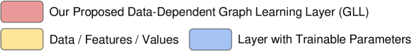
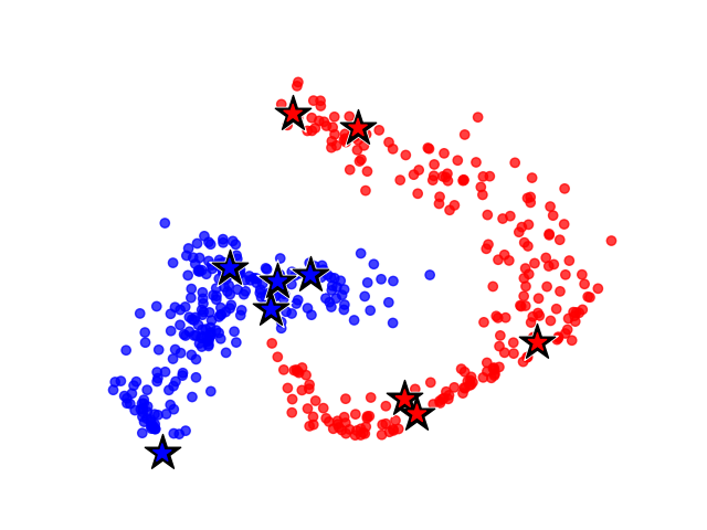
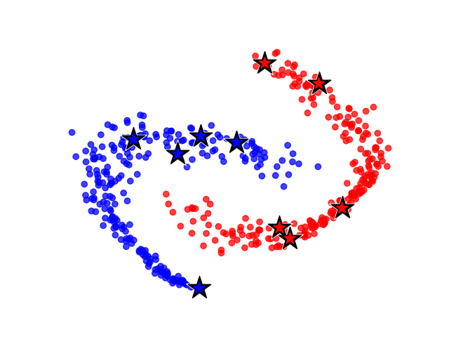
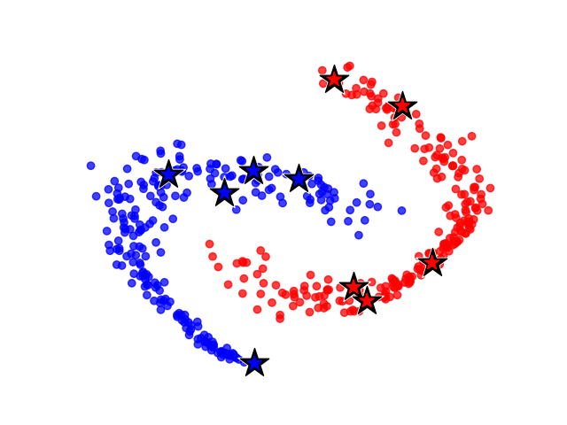
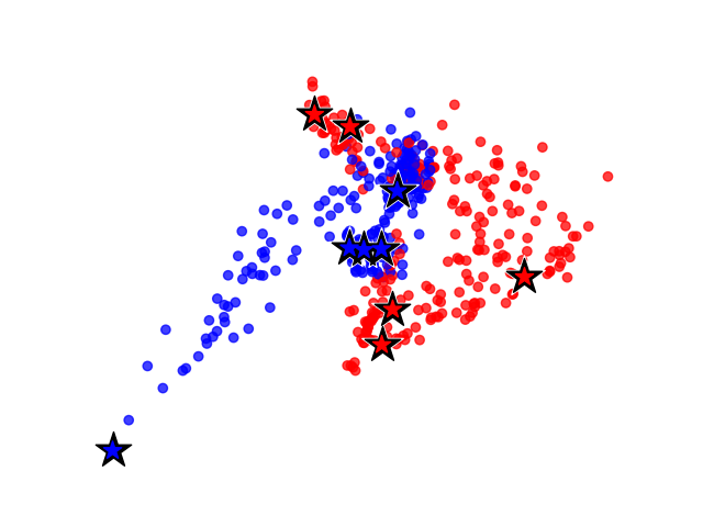
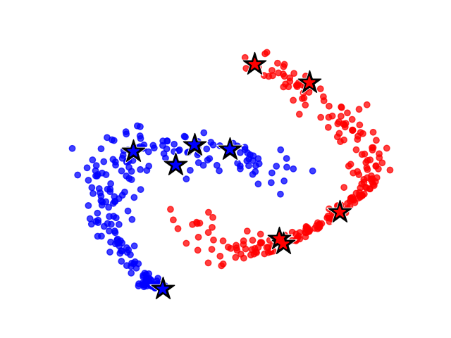
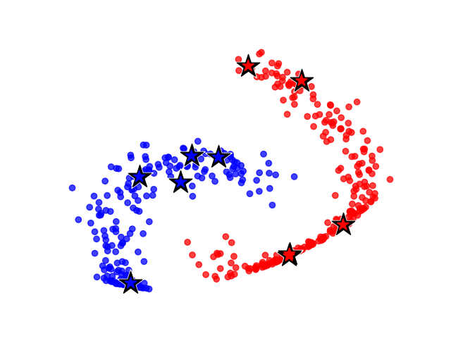
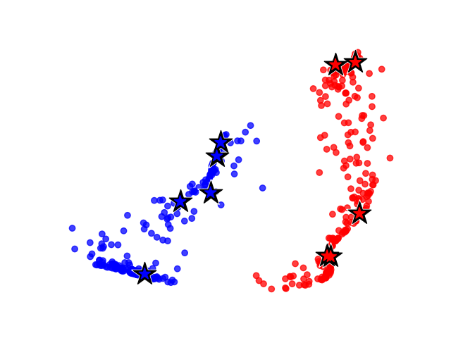
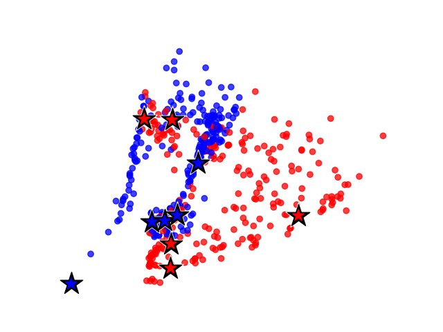
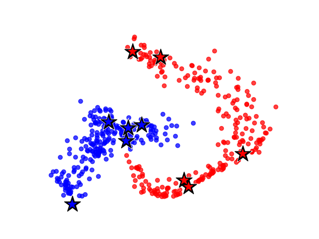
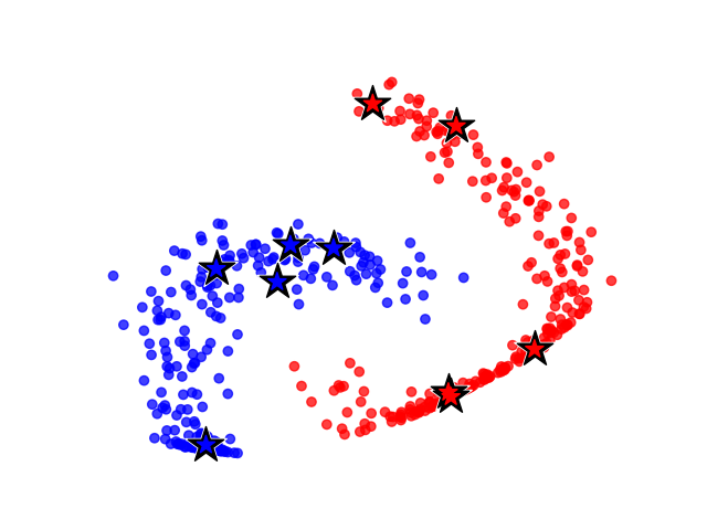
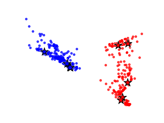
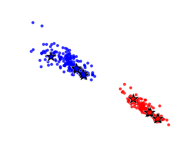
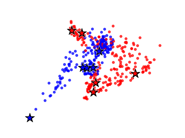
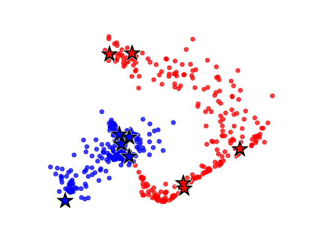
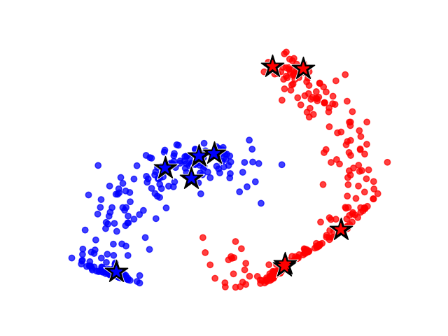
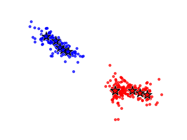
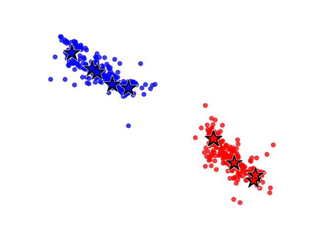
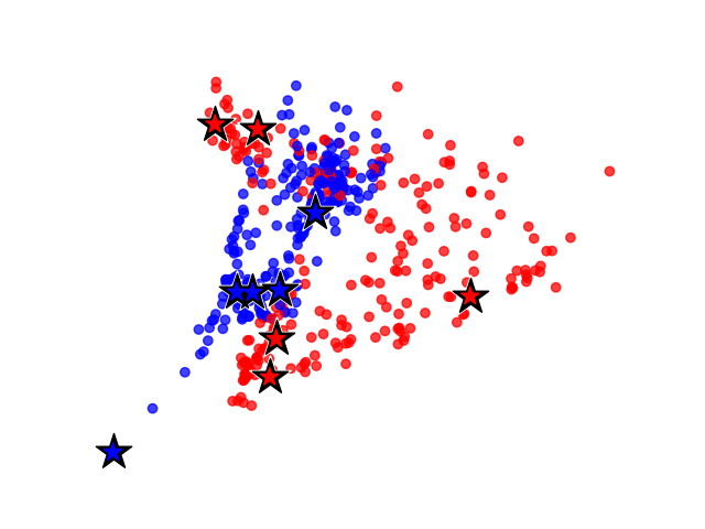
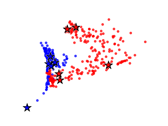
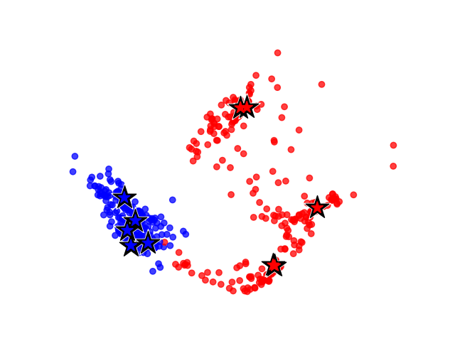
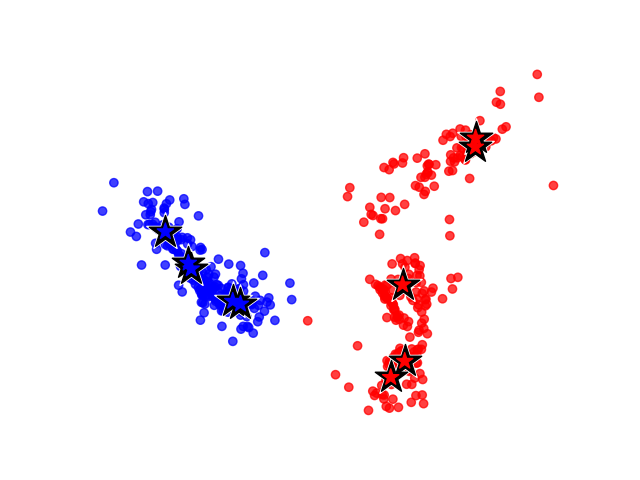
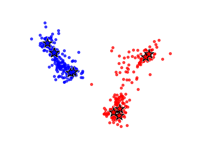
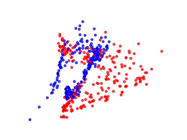
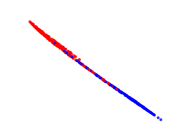
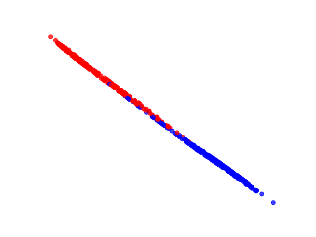
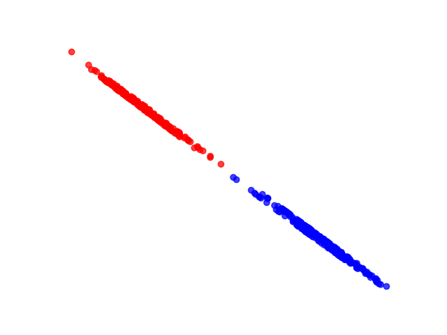
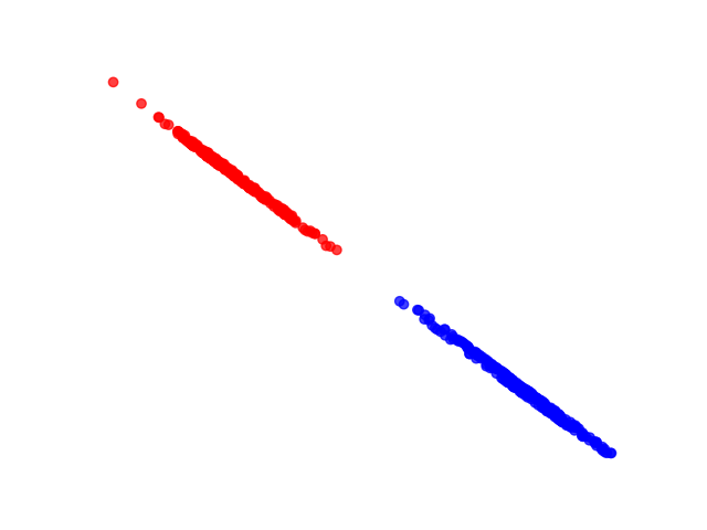
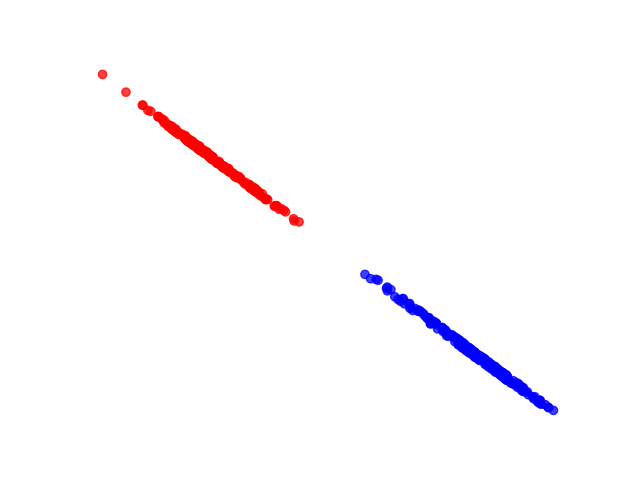
In this subsection, highlight the differences between the learned embeddings of neural networks when trained on GLL compared to a softmax-based classifier. When trained with GLL, the neural network’s latent space recovers the underlying geometry of the data, which may be desireable for applications. Moreover, we visualize the effect on the decay parameter from Section 2.4. Larger values of result in tighter clustering of the data in the latent space, at the expense of preserving the geometry. The tradeoff between these two will depend on the application; for now, we give a brief example with a toy dataset (two moons (Pedregosa et al. (2011))).
The architecture backbone for this experiment is a multi-layer perceptron neural network with three linear layers. The hidden size is 64 and the output size is two for two dimensional visualization purposes. We choose an initialization where the samples are sufficiently mixed, making the problem more difficult (Figure 2). We arbitrarily choose the first ten samples as the labeled samples from which GLL will propagate the labels. We use cross entropy loss. To make the results more interpretable, we fix the term to be one. The embeddings for this ablation study is shown in Figure 3. We compare five values of : 0, 0.001, 0.01, 0.1, and 0.5. The figure shows the learned embedding of the dataset from the neural network across various training epochs.
We note that this regime is deliberately constrained to two dimensions, meaning the data will struggle to move past each other in the latent space. The seed for these samples was chosen to be difficult and has the a very mixed initialization for the sample embeddings. Despite this, after sufficient training, the model successfully separates the data.

| Ep. 0 | Ep. 500 | Ep. 2e3 | Ep. 1e4 | Ep. 5e4 | Ep. 1.5e5 | |
|
|

|
|
|
|
|
|

|
|

|
|
|
|
|
|

|
|
|
|
|
|

|
|
|
|
|
|
|

|
|
|
|
|
|
|
| Softmax |
|
|
|
|
|
|
These experiments highlight the geometry of the learned embeddings under GLL. We compare these embeddings to the ones learned by the same three layer MLP encoder network but with a projection head and softmax layer in place of the GLL layer. The baseline MLP encoder with the projection head will simply linearly separate the data. The encoder immediately followed by the GLL layer, however, will quickly recover the original two moons shape. The addition of the decay parameter will encourage tighter clustering of the classes around the base labels, rather than a two moons shape. For low values of , we still see initial convergence to the two moons, since the driving loss term comes from label predictions. Once the two moons structure is reached, the loss from the prediction is negligible and the regularization term begins to drive the loss, which results in tighter clusters. If the value is too large, then the two moons shape is skipped entirely in favor of a tighter clustering. A large value could also cause the labeled groups to splinter into multiple clusters localized about different base samples.
4.2 Comparison to the Multilayer Perceptron (MLP)
One direct application of our proposed GLL is to serve as a classifier, replacing a projection layer and softmax. In Figure 1, we illustrate the differences between the neural network structure incorporating our GLL and the standard structure. Since GLL does not include any trainable parameters, the reduced number of parameters and layers makes our network structure smoother to train. In this subsection, we design experiments to compare the performance of using an MLP and our GLL as classifiers under the same feature encoder. We conclude that by replacing the MLP with GLL as the classifier in classic network structures, the training speed of the network will be accelerated, and it can effectively avoid problems such as training stagnation caused by vanishing gradients.
We consider two datasets, the FashionMNIST dataset (Xiao et al. (2017)) and the CIFAR-10 dataset (Krizhevsky et al. (2009)), for the experiments in this section. For the FashionMNIST dataset we use a simple CNN-based network (Table 1) with a feature encoder containing 3 convolutional layers (Conv) and 1 fully connected layer (FC). Each conv and FC layer is followed by a corresponding ReLU activation function, which is omitted in the table. On the CIFAR-10 dataset, we employ standard ResNet-18 and ResNet-50 architectures, where the feature encoder consists of several ResNet blocks followed by an FC layer (Table 2). For both datasets, the MLP Classifiers consist of 2 FC layers followed by a softmax layer. To compare with our GLL layer, we keep the feature encoder structure unchanged from Tables 1,2 and replace the MLP classifier with the GLL classifier. The outputs are used to calculate the cross-entropy loss with the ground-truth labels and perform backpropagation and optimization.
We also compare with the neural networks trained with weighted nonlocal Laplacian (WNLL, Wang and Osher (2021)), called WNLL-DNN, on the CIFAR-10 dataset. WNLL-DNN uses a graph-based classifier, but approximates the gradients using a linear layer. We used the accuracy values of ResNet-18 and ResNet-50 reported in their paper. The detailed network architecture for WNLL-DNN can be obtained from their GitHub repository 555https://github.com/BaoWangMath/DNN-DataDependentActivation/tree/master. The only difference between our ResNet architecture (Table 2) and theirs is the number of parameters in the fully connected layers after the ResNet blocks.
| Structure | Layer | Details | Feature Size |
| Input Image | - | From FashionMNIST Dataset | 28 28 1 |
| Feature Encoder | Conv1 | 1 64, kernel size: 3, padding: 1 | 28 28 64 |
| Conv2 | 64 128, kernel size: 3, padding: 1 | 28 28 128 | |
| MaxPool | kernel size: 2, stride: 2 | 14 14 128 | |
| Conv3 | 128 256, kernel size: 3, padding: 1 | 14 14 256 | |
| MaxPool | kernel size: 2, stride: 2 | 7 7 256 | |
| FC | 256 7 7 128 | 128 | |
| MLP Classifier | FC1 | 128 1024 | 1024 |
| FC2 | 1024 10 | 10 | |
| Softmax | dim: 1 | 10 |
| Structure | Layer | Details | Feature Size |
| Input Image | - | From CIFAR-10 Dataset | 32 32 3 |
| Feature Encoder | ResNet-18 | 8 ResNet Blocks | |
| or ResNet-50 | ResNet Blocks | ||
| FC | 512/2048 128 | 128 | |
| MLP Classifier | FC1 | 128 32 | 32 |
| FC2 | 32 10 | 10 | |
| Softmax | dim: 1 | 10 |
All experiments in this section are fully supervised with the entire training set of the FashionMNIST and CIFAR-10 datasets. We report results on the following experiments:
-
•
(FashionMNIST: 100 MLP) Directly training a neural network with an MLP Classifier from scratch. In this case, we simultaneously record the training loss and test accuracy of both the MLP and GLL during the training process. Specifically, the output of the Feature Encoder is passed to both the MLP Classifier and a GLL. Since GLL has no parameters, this does not affect the training. Then, based on the output of this GLL, we can calculate the GLL loss/accuracy during the MLP training process. Here, we train for 100 epochs.
-
•
(FashionMNIST: 50 GLL) Training a neural network with GLL as the classifier from scratch, only training for 50 epochs.
-
•
(FashionMNIST: 50 MLP + 50 GLL) Starting from the 50th epoch of the MLP training process, we switch to using the backpropagation gradient information from the GLL Classifier for training and continue training for another 50 epochs.
-
•
(FashionMNIST: 75 MLP + 25 GLL) Starting from the 75th epoch of the MLP training process, we switch to using GLL for training and continue training for another 25 epochs.
-
•
(CIFAR-10 MLP and GLL) We pretrain the feature encoder on the CIFAR-10 training dataset using the SimCLR method, which does not require any label information. Subsequently, we use these SimCLR weights as the initial weights for the feature encoder, combined with either an MLP classifier (PyTorch’s default weight initialization) or our GLL classifier (no trainable parameters) to perform fully supervised training. More details about training on CIFAR-10 are in Appendix A.
-
•
(CIFAR-10 WNLL-DNN) We use the accuracy values reported in the paper (Wang and Osher (2021)).
| Dataset | Trial | Network | Epochs | Accuracy |
|---|---|---|---|---|
| FashionMNIST | MLP Only | Customized | 100 MLP | 54.58% MLP |
| 85.34% GLL | ||||
| GLL Only | 50 GLL | 91.10% GLL | ||
| GLL-50 | 50 MLP + 50 GLL | 91.32% GLL | ||
| GLL-75 | 75 MLP + 25 GLL | 91.09% GLL | ||
| CIFAR-10 | MLP | ResNet-18 | 800 MLP | 95.42% MLP |
| GLL | 800 GLL | 96.10% GLL | ||
| WNLL-DNN | N/A | 95.35% WNLL | ||
| MLP | ResNet-50 | 800 GLL | 95.77% MLP | |
| GLL | 800 GLL | 96.54% GLL | ||
| WNLL-DNN | N/A | 95.83% WNLL |
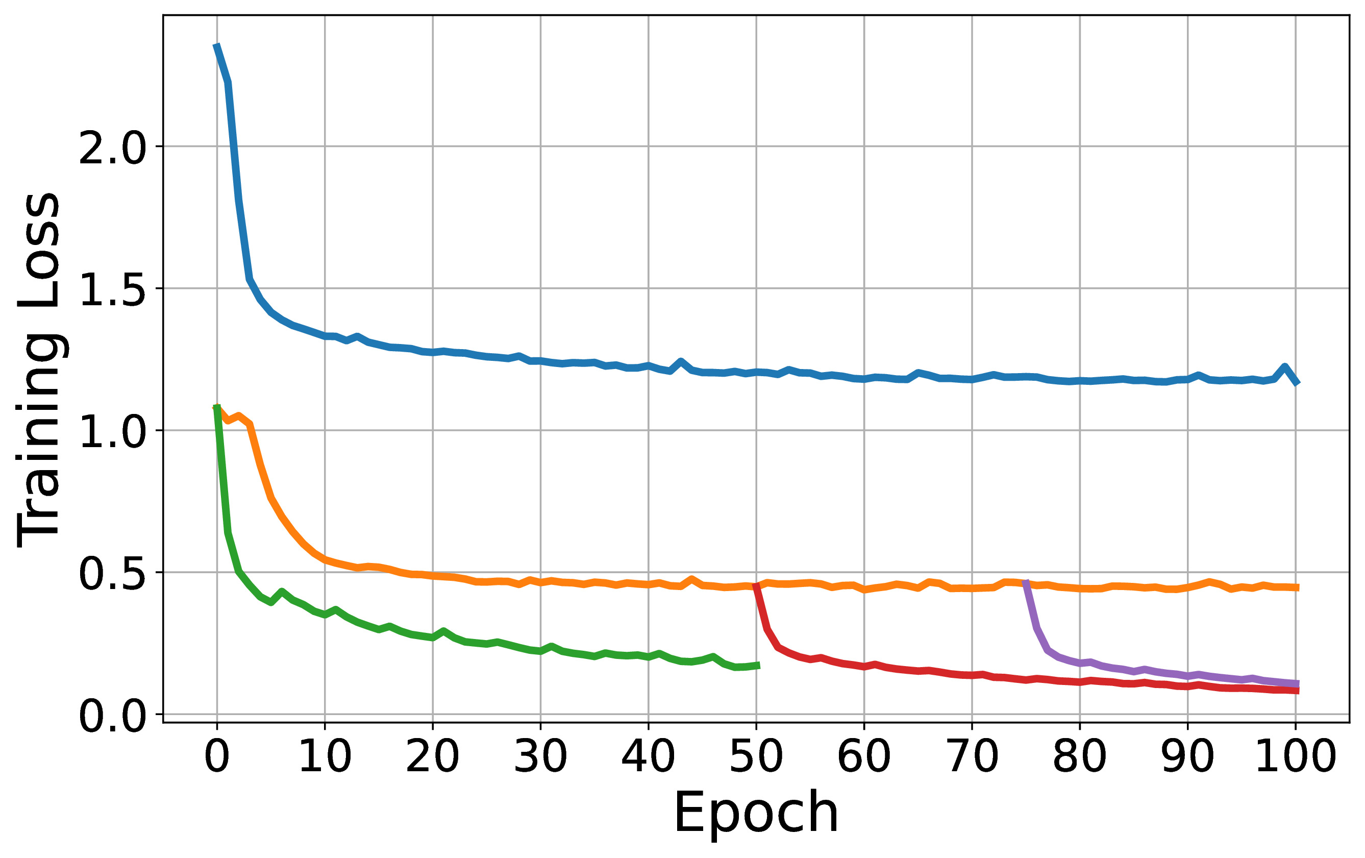
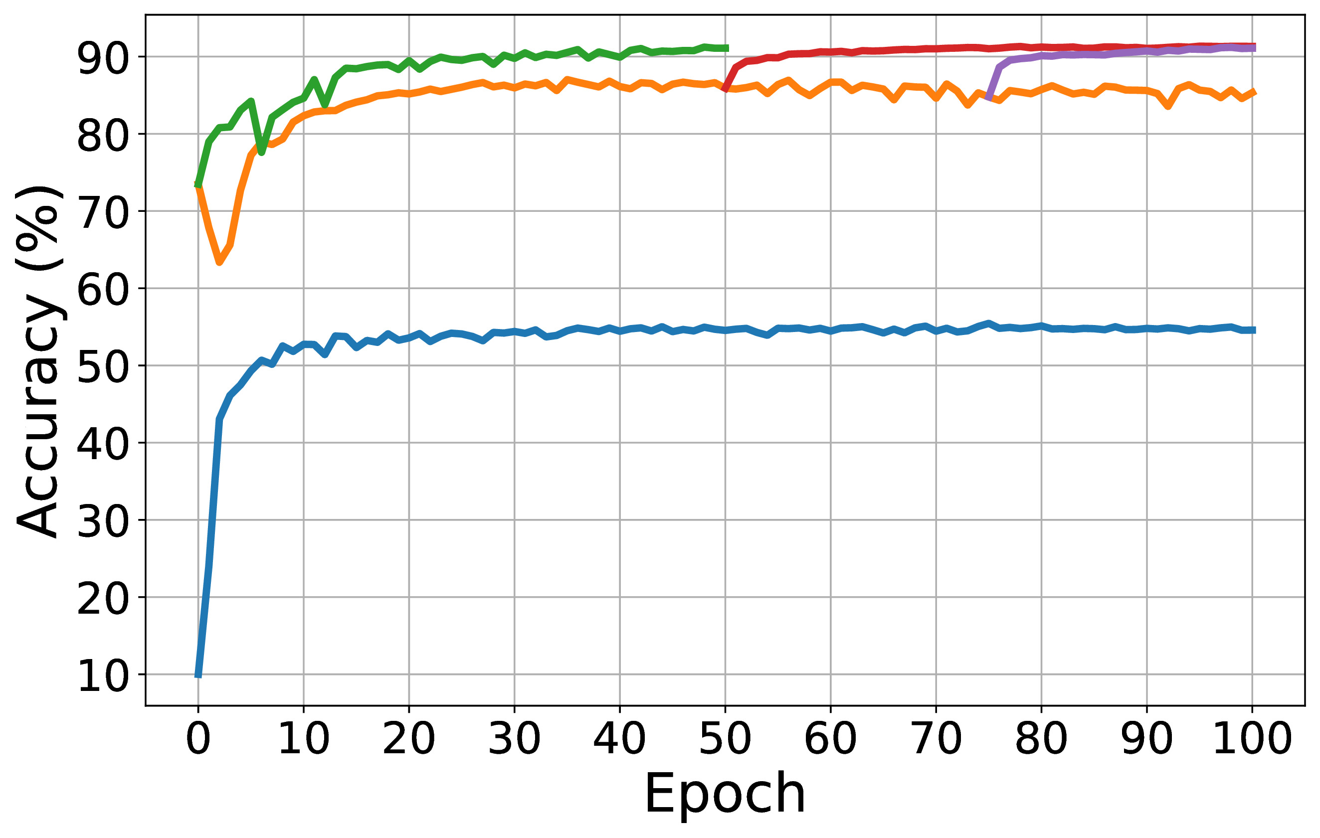
Accuracy comparison is shown in Table 3. For the FashionMNIST results, we provide Figure 4, which compares the four training strategies. Figure 4(a) presents the training loss curves as the epochs progress, while Figure 4(b) displays the test accuracy curves over the epochs. Since GLL-50 and GLL-75 are trained after 50 and 75 epochs of MLP training, respectively, their corresponding curves do not start from 0.
From Table 3, it is evident that our customized neural network, as shown in Table 1, performs poorly. Several factors could contribute to the poor performance of the customized neural network. First, the high number of parameters significantly increases the risk of overfitting, particularly on a relatively small dataset like FashionMNIST. Second, the complex architecture, with multiple convolutional and fully connected layers, may lead to optimization challenges such as vanishing or exploding gradients, especially in deeper layers. Third, the lack of advanced regularization techniques, such as dropout or weight decay, might exacerbate the model’s inability to balance learning and generalization. Fourth, the computational demands of the large model might lead to slower convergence, requiring more training epochs and careful hyperparameter tuning. Based on the results, the primary reason for the poor performance appears to be vanishing gradients or the slower convergence. When the MLP classifier is replaced with the GLL classifier while keeping the same network structure, the performance improves significantly with the same feature encoder architecture. More details are discussed below.
We summarize the main takeaways of this experiment:
-
1.
Accuracy comparison: In Table 3, networks with our GLL classifier have better accuracy than the MLP classifier under the same feature encoder structure, where the MLP classifier can be training directly or under the WNLL strategy. On the CIFAR-10 dataset, using ResNet architectures, replacing the MLP with GLL yields a modest improvement in accuracy. On the FashionMNIST dataset, where we employ our custom network, the improvement is more substantial. Our MLP accuracy on the CIFAR-10 dataset is similar to the WNLL accuracy, which is higher than the vanilla training results reported in the WNLL paper (Wang and Osher (2021)). One possible reason is that we incorporated SimCLR pretraining during the network training process, which provided a better initialization for the subsequent fully supervised training, resulting in improved performance.
-
2.
Difference between MLP and GLL loss and accuracy in the MLP training: According to the FashionMNIST training curves (Figure 4), for MLP training (blue and orange curves), we provide both the MLP and GLL loss and accuracy during the training process. We observe that under the same feature encoder, the output of GLL corresponds to lower loss values and higher accuracy. This indicates that even if the information from GLL does not participate in the training, directly replacing MLP with GLL can achieve a significant improvement in performance. One reason is that the MLP classifier contains a large number of trainable parameters, which do not have a good classification effect when not well-trained. Another reason is that, even when well-trained, an MLP classifier consisting of several FC layers and ReLU activation functions can be understood as a series of hyperplanes that partition the feature space into classification regions (Montufar et al. (2014); Goodfellow et al. (2016)). While this approach can be effective, it may not fully capture the intrinsic structure of the data. In contrast, GLL’s Laplace Learning leverages the manifold structure of the data to guide the classification process. By considering the relationships between data points and their neighbors, GLL can potentially learn more complex and non-linear decision boundaries that better align with the underlying data distribution. This allows GLL to achieve superior classification performance compared to the hyperplane-based approach of MLP classifiers.
-
3.
Smooth training and improved convergence with GLL: In Figure 4, GLL-0, trained from scratch, achieves good accuracy and low loss function in a short time, and the performance continues to improve slowly as the training progresses (up to 50 epochs). It is worth noting that the training of MLP quickly stagnates, with the loss and accuracy showing little change over a long period. However, the training continues very smoothly when we replace the MLP training process with GLL midway, i.e., GLL-50 and GLL-75. One possible explanation of this phenomenon is if the number of parameters or the number of layers is large, it may lead to the dying ReLU problem (Lu et al. (2020)) or vanishing gradients (Hochreiter (1998)), causing training stagnation. On the other hand, since GLL does not contain any trainable parameters, it can make the optimization process more smooth.
4.3 Adversarial Robustness
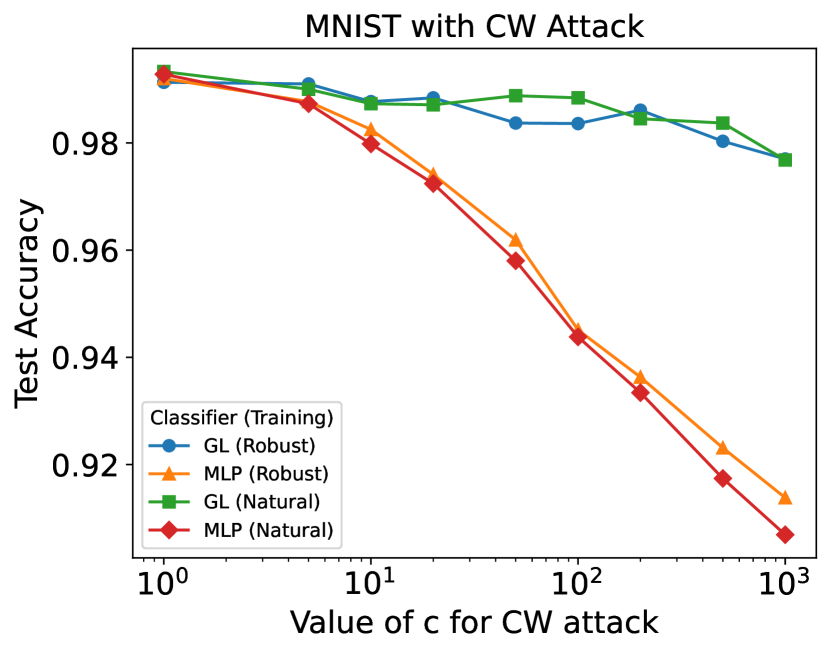
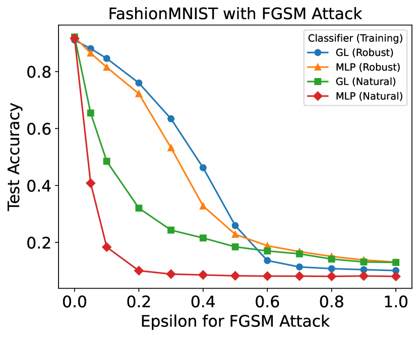
In this subsection, we demonstrate our method’s superior robustness to adversarial attacks compared to the typical projection head and softmax activation layer in a neural network. Adversarial attacks seek to generate adversarial examples (Szegedy et al. (2013)): input data with small perturbations that cause the model to misclassify the data. Many highly performant deep neural networks can be fooled by very small changes to the input, even when the change is imperceptible to a human (Madry et al. (2017); Goodfellow et al. (2014)). Hence, training models robust (i.e. resistant) to such attacks is important for both security and performance. Our experiments show that in both naturally and robustly-trained models, using the graph learning layer improves adversarial robustness compared to a softmax classifier on MNIST (Yann LeCun (2010)), FashionMNIST (Xiao et al. (2017)), and CIFAR-10 (Krizhevsky et al. (2009)) in both relatively shallow and deep networks. Moreover, GLL is more robust to adversarial attacks without sacrificing performance on natural images.
4.3.1 Adversarial Attacks
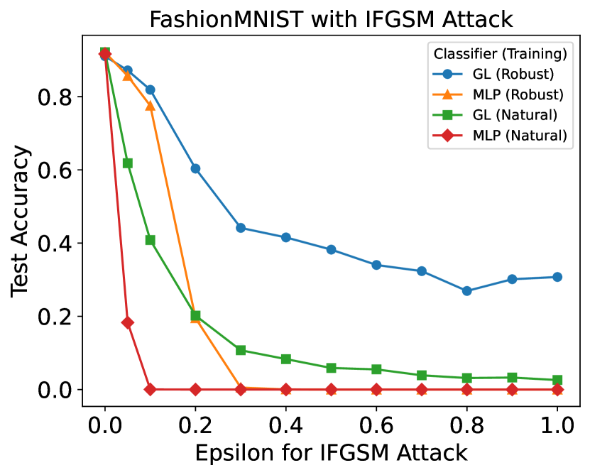
We consider three types of adversarial attacks: the fast gradient sign method (FGSM) (Goodfellow et al. (2014)) in the norm, the iterative fast gradient sign method (IFGSM) (Kurakin et al. (2018)) in the norm, and the Carlini-Wagner attack (Carlini and Wagner (2017)) in the norm.
The FGSM and IFGSM attacks consider the setting where an attacker has an “budget” to perturb an image . More formally, FGSM creates an adversarial image by maximizing the loss subject to a maximum allowed perturbation , where is a hyperparameter. Thus, a larger is more likely to successfully fool a model, but also more likely to be detectable. We can linearize the objective function as
which gives the optimal (in this framework) adversarial image
| (43) |
It is also standard to clip the resulting adversarial example to be within the range of the image space (e.g. for grayscale images) by simply reassigning to .
Intuitively, FGSM computes the gradient of the loss with respect to each pixel of to determine which direction that pixel should be perturbed to maximize the loss. It should be noted that, as the name suggests, FGSM is designed to be a fast attack (the cost is only one call to backpropagation), rather than an optimal attack.
IFGSM simply iterates FGSM by introducing a second hyperparameter , which controls the step size of the iterates:
where and , and so is the generated adversarial example. However, we must also clip the iterates (pixel-wise) during this iteration to ensure that (1) they remain in the -neighborhood of and (2) they remain in the range of the image space (e.g. in [0,1] for a grayscale image). Thus, the IFGSM attack is:
| (44) |
where
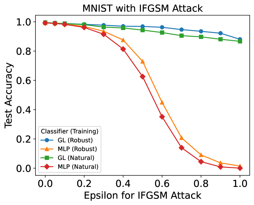
Note that this assumes the pixel values are in the range , but can be easily tailored to other settings. IFGSM attacks have been shown to be more effective than FGSM attacks (Kurakin et al. (2018)), however we will see in Section 4.3.3 that our graph learning layer is highly robust to this iterative method.
CW attacks frame the attack as an optimization problem where the goal is to find a minimal perturbation that changes the model’s classification of an input . Let be the neural network, so that gives a discrete probability distribution over classes for an input . Let be the classification decision for . The CW attack is a perturbation that solves:
| s.t. | |||
where is a classification such that . In other words, the CW attack seeks a minimal perturbation to apply to that changes its classification (while remaining a valid image). Other norms on are possible; in this work we focus on the norm. In practice, we choose to be the class with the second highest probability in , i.e.
The constraint is highly non-linear, so Carlini and Wagner instead consider objective functions that satisfy if and only if . While there are many choices for (see Carlini and Wagner (2017), Section IV A), we will use the following in our experiments:
where . It is worth noting that a common choice for in the literature is to use the unnormalized logits from the neural network (that is, the output of a neural network just before the standrad softmax layer) instead of . While both definitions satisfy the condition, we use the above because graph learning methods (such as Laplace learning) operate in the feature space and directly output probability distributions over the classes, so there is no notion of logits.
Using , we can reformulate the problem as
| s.t. |
where is a suitably chosen hyperparameter. To make the problem unconstrained, we can introduce a variable and write ; since , we have that . This gives the unconstrained objective:
| (45) |
which can be solved using standard optimization routines; we use the Adam optimizer (Kingma and Ba (2014)).
4.3.2 Adversarial Training
To train adversarially robust networks, we use projected gradient descent (PGD) adversarial training (Madry et al. (2017)) to our models. Motivated by guaranteeing robustness to first-order adversaries, PGD training applies IFGSM to images with an random initial perturbation during training. Hence, the model is trained on adversarial examples. More precisely, PGD training consists of two steps each batch: first, is randomly perturbed
where is a uniform random perturbation. Then, IFGSM is applied
where and the number of iterations and are hyperparameters. This training procedure, while more expensive, has been shown to be effective at improving robustness in deep learning models compared to training on clean (i.e. natural) images (Madry et al. (2017), Wang and Osher (2021)).
4.3.3 Adversarial Experiments
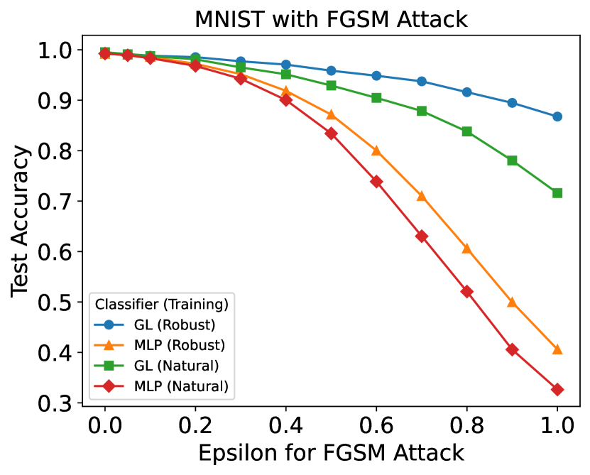
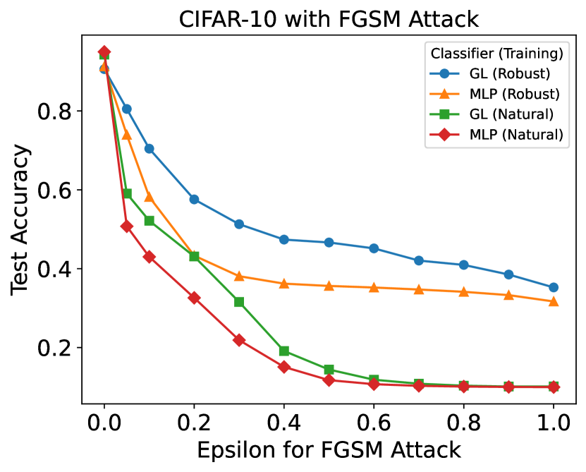
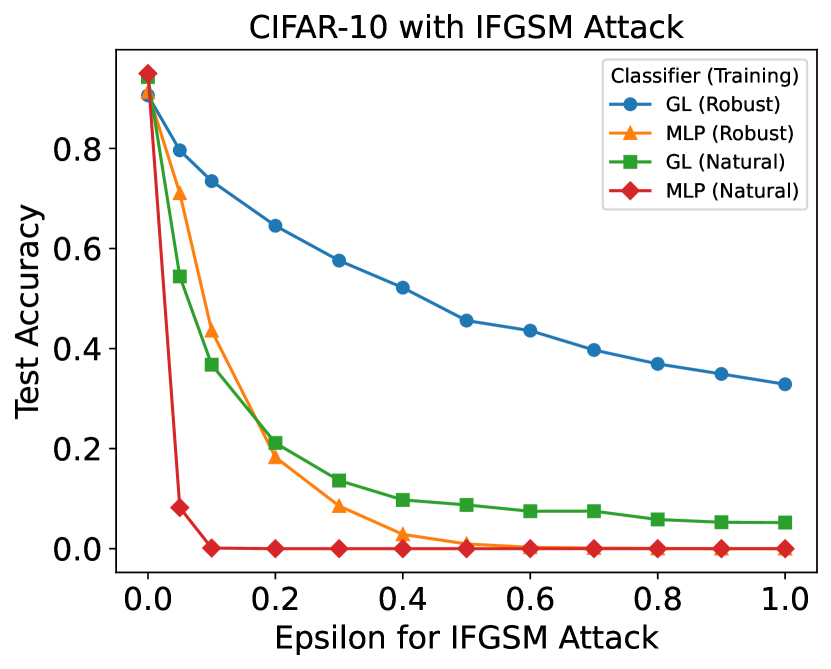
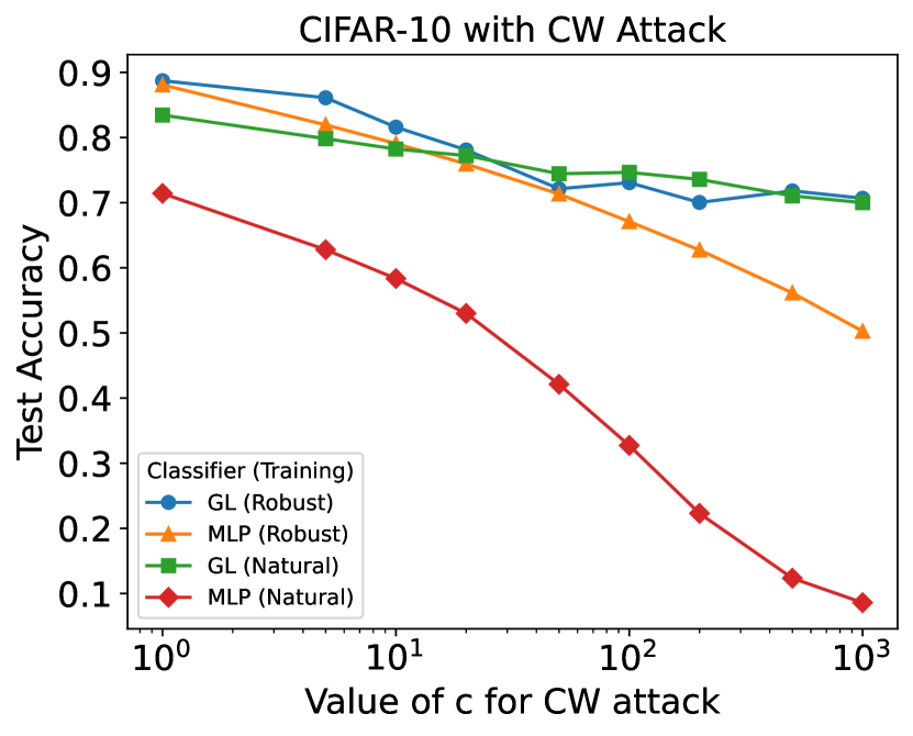
We evaluate the adversarial robustness of neural networks with the GLL classifier on the MNIST (Yann LeCun (2010)), FashionMNIST (Xiao et al. (2017)), and CIFAR-10 (Krizhevsky et al. (2009)) benchmarks datasets, and compare our method to the same networks with a softmax classifier. For all datasets, we normalize the images to have mean 0 and standard deviation 1, and we train and run all adversarial attacks on a 11GB GeForce RTX 2080Ti GPU. We note that the goal of these experiments is not to get state-of-the-art natural accuracies; while our natural accuracy on these benchmark datasets is strong, the purpose of these experiments is to demonstrate our method’s superior robustness to adversarial attacks compared to the typical classifier (a linear layer and softmax layer), on a variety of networks and datasets, without sacrificing performance on natural images. A summary of our experiments - highlighting a handful of our adversarial robustness results - can be found in Table 4, while complete results are shown in Figures 5, 6, and 7. Throughout, when we say “MLP” we mean a linear layer mapping from the feature space to the logits followed by a softmax classifier, while “GLL” refers to our graph learning layer classifier.
| Dataset | Model | Natural | FGSM | IFGSM | CW |
|---|---|---|---|---|---|
| MNIST | GL Robust | 99.45 | 97.72 | 97.70 | 98.84 |
| MLP Robust | 99.20 | 95.17 | 93.57 | 97.41 | |
| GL Natural | 99.53 | 96.51 | 96.44 | 98.71 | |
| MLP Natural | 99.25 | 94.26 | 91.52 | 97.24 | |
| Fashion-MNIST | GL Robust | 91.04 | 88.07 | 87.17 | 83.81 |
| MLP Robust | 92.08 | 86.50 | 85.67 | 81.00 | |
| GL Natural | 92.14 | 65.44 | 61.81 | 57.19 | |
| MLP Natural | 91.65 | 40.81 | 18.30 | 62.01 | |
| CIFAR-10 | GL Robust | 90.60 | 80.50 | 79.62 | 78.09 |
| MLP Robust | 91.29 | 73.95 | 71.04 | 75.94 | |
| GL Natural | 94.29 | 59.05 | 54.41 | 77.23 | |
| MLP Natural | 94.98 | 50.75 | 8.21 | 53.00 |
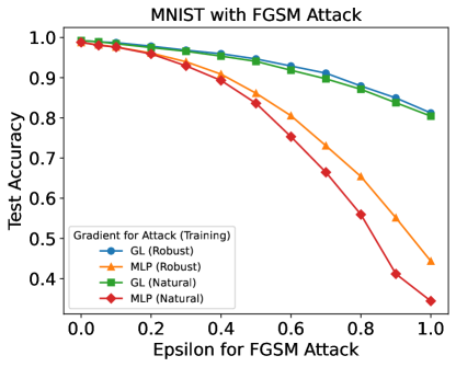
For MNIST, we use the same “small CNN” architecture as in Wang and Osher (2021): four convolutional layers with ReLU activations after each layer and maxpooling after the 2nd and 4th layer, followed by 3 linear layers and a softmax classifier. To adopt this CNN to our approach, we replace the final linear layer and softmax with our GLL. We train for 100 epochs using the Adam optimizer (Kingma and Ba (2014)) with an initial learning rate of which decays by a factor of every 25 epochs. For the robustly trained models, we run PGD training with and for 5 iterations. In training, we use a batch size of 1000, and for GLL we use 100 labeled “base” points per batch (i.e. 10 per class), which are randomly sampled each epoch.
To evaluate experimental robustness, we attack the test set with the FGSM, IFGSM, and CW attacks. When using FGSM and IFGSM on GLL, we embed the entire test set of 10000 digits along with 10000 randomly selected data points from the training set (i.e. 1000 per class) when running the attacks, while we run CW in batches of 1000 test and 1000 training points (this was simply due to computational constraints; in general graph learning methods perform better with more nodes on the graph as it better approximates the underlying data manifold). For the models with MLP classifier, we use the same batch sizes (full batch on FGSM and IFGSM, 1000 for CW). We report results for FGSM and IFGSM at varying levels of , fixing for IFGSM and letting the number of iterations be , following a similar heuristic as in Kurakin et al. (2018) to allow the adversarial example sufficient ability to reach the boundary of the -ball. For CW attacks, we let vary and run 100 iterations of the Adam optimizer with a learning rate of 0.005. Results for each attack, comparing both robustly and naturally trained models with MLP and GLL classifiers, are shown in Figure 5.
For FashionMNIST, we use ResNet-18 (He et al. (2016a)), where again we replace the final linear layer and softmax with GLL. We again use the Adam optimizer for 100 epochs, with an intial learning rate of which decays by a factor of every 10 epochs. For the robustly trained models, we run PGD training with and for 5 iterations. In training, we use a batch size of 2000, and for GLL we use 200 labeled “base” points per batch. We attack in batches of 250 test points, with 500 training points for GLL; this was chosen as it was the largest batch size we could use given our computational resources. The hyperparameters for the attacks are identical to those for MNIST. We report results in Figure 6.
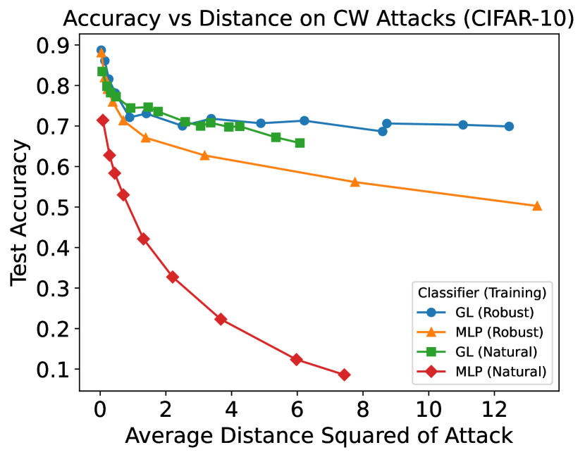
Finally, for CIFAR-10, we use PreActResNet-18 (He et al. (2016b)), where again we replace the final linear layer and softmax with GLL. We use stochastic gradient descent with momentum set to , a weight decay of , and an intial learning rate of . We train for 150 epochs and use cosine annealing to adjust the learning rate (Loshchilov and Hutter (2016)). For the robustly trained models, we run PGD training with and for 5 iterations. In training, we use a batch size of 200, and for GLL we use 100 labeled “base” points per batch. We attack in batches of 200 test points, with 500 training points for GLL; this was chosen as it was the largest batch size we could use given our computational resources. The hyperparameters for the attacks are identical to those for MNIST, except we use 50 iterations of optimization for the CW attacks. We report results in Figure 7.
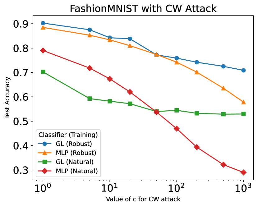
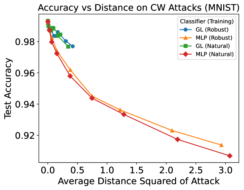
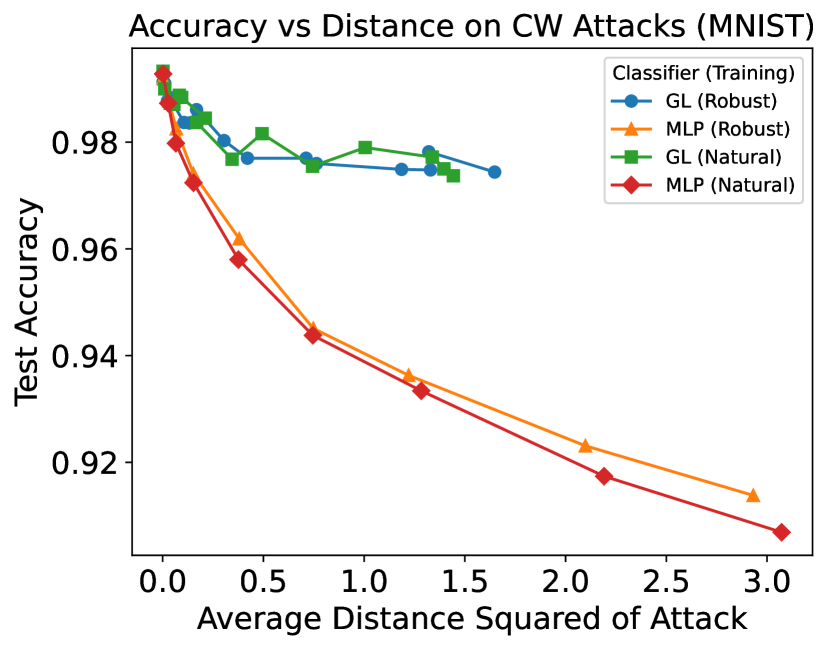
We further investigate the performance of GLL against CW attacks in Figure 8. This figure plots the accuracy versus the average distance (squared) that the adversary moves an image in the test set (instead of the value of ). This reveals a striking difference between MLP and GLL: GLL resists the CW adversary from moving the images significantly more than the MLP classifier, making it more robust to these attacks. The one exception is the FashionMNIST robust GLL model, which still outperforms the MLP-based model across distances and values of .
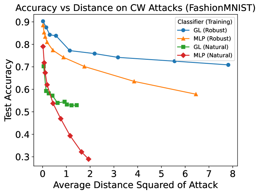
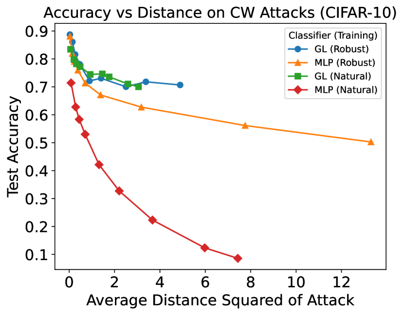
We see that, across datasets, training methods (both natural and robust), severity of attacks, and neural network architectures, our graph learning layer is significantly more robust to adversarial attacks, notably without sacrificing in natural accuracy. Laplace learning can be viewed as repeatedly computing a weighted average over a given node’s neighbors, and this relational information may be preventing attacks from successfully perturbing the input images to fool the network. In particular, we note that the models employing the standard classifier quickly decay to 0 accuracy against IFGSM and CW attacks, while GLL shows robustness to these attacks, even for extremely large values of and , respectively. Moreover, performance of our GLL could likely be even further improved with more computational resources, as graph learning techniques tend to improve as the number of nodes (i.e. the batch size) increases.
5 Conclusion
Graph-based learning is a powerful class of machine learning techniques that have been developed throughout the 21st century. As research in deep learning has exploded throughout the same time period, there has been significant interest in integrating deep learning with similarity matrix-based graph learning. This paper gives a precise mathematical framework to do exactly that. We derived the necessary gradient backpropagation equations for general nonlinear elliptic graph Laplace equations, allowing us to fully integrate graph-based classifiers into the training of neural networks. Using this novel framework, we introduced the Graph Learning Layer, or GLL, which replaces the standard projection head and softmax classifier in classification tasks. Experimentally, we demonstrated how GLL improves upon the standard classifier in several ways: it can learn the geometry underlying data, it can improve the training dynamics and test accuracy on benchmark datasets in both small and large networks, and it is significantly more robust to a variety adversarial attacks in both naturally and robustly trained models.
There are many exciting avenues of future work in this area. Given the strong empirical results, theoretically guaranteeing the adversarial robustness of GLL is an important extension of this work. Graphs are a common setting for active learning techniques Settles (2009); Miller and Bertozzi (2024); the full integration of graph learning into a neural network provides a natural way to do active learning in a deep learning context. Our theoretical work also provides a way to integrate other graph learning algorithms - such as -Laplace learning and Poisson learning - into a deep learning framework, and numerical experiments could yield similarly strong results as reported in this paper. Many performant semisupervised deep learning techniques utilize psuedolabels generated by graph learning methods Iscen et al. (2019); Sellars et al. (2021); we hope the methods presented here will lead to further improvements and insights.
Acknowledgments and Disclosure of Funding
HHM and JB were partially supported by NSF research training grant DGE-1829071. HHM was supported by the National Science Foundation Graduate Research Fellowship Program under Grant No. DGE-2034835. JB and ALB were also supported by Simons Math + X award 510776. ALB and BC were supported by NSF grants DMS-2027277 and DMS-2318817. BC was supported by the UC-National Lab In- Residence Graduate Fellowship Grant L21GF3606. JC was supported by NSF-CCF:2212318, the Alfred P. Sloan Foundation, and an Albert and Dorothy Marden Professorship. Any opinions, findings, and conclusions or recommendations expressed in this material are those of the author and do not necessarily reflect the views of the National Science Foundation. The authors declare no competing interests.
Appendix A Training Details
This section provides a detailed discussion of various aspects of the training process. These details are implemented in our experiments (Section 4), especially in the fully-supervised training for comparison between the MLP and GLL classifiers (Section 4.2).
Prior to GLL-based fully supervised training for the CIFAR-10 dataset, we initialize the network’s feature encoder using pre-trained weights from SimCLR (Chen et al. (2020a, b)). SimCLR is a framework for contrastive learning of visual representations. For a neural network and a minibatch of samples , each is augmented into pairs . These are processed through the network: . The SimCLR loss is defined as:
| (46) |
where is a temperature parameter, and is the cosine similarity. It is worth noting that the cosine similarity used in the SimCLR loss (46) closely resembles the similarity measure we employ when constructing graphs in graph Laplace learning. This similarity suggests that the feature vectors generated by a network trained with SimCLR already possess a favorable clustering structure. Consequently, utilizing SimCLR to pretrain the feature encoder in our network can significantly reduce the difficulty of subsequent training stages.
We employed augmentation techniques in both the SimCLR pre-training process and the subsequent fully supervised training. For data augmentation in both stages, we utilized the strong augmentation method defined in the SupContrast GitHub Repository666https://github.com/HobbitLong/SupContrast/tree/master. The use of data augmentation is helpful for two main reasons. Firstly, in contrastive learning, augmentation creates diverse views of the same instance, which is fundamental to learning robust and invariant representations. This process helps the model to focus on essential features while disregarding irrelevant variations. Secondly, for general training tasks, augmentation enhances the model’s ability to generalize by exposing it to a wider variety of data representations, thereby reducing overfitting and improving performance on unseen data.
In the GLL-based fully supervised training process, our approach differs from classic training methods. For each minibatch, in addition to batch images and their corresponding labels, we also require base images and their associated base labels. While this base data can remain fixed throughout the entire training process, updating the base dataset during training can enhance the overall effectiveness. The base dataset in graph Laplace learning represents the labeled nodes, which can also be viewed as the sources in a label propagation process. An ideal base dataset should be relatively dispersed and distributed near the decision boundaries of different clusters.
Let denote the training dataset, and be the number of base data points. We can simply update the based dataset as a random subset such that . Or we can define a score to evaluate which data is more beneficial if selected. Assume that at a certain epoch, the Laplace learning output for is , where is the total number of classes. We can define two types of scores that essentially measure the uncertainty of the output :
| Entropy score | (47) | |||
| L2 score | (48) |
We then select the base dataset as the data with the highest scores. However, there’s a possibility that the selected high-score data points may cluster together in the graph structure, potentially providing redundant information. A better approach is to employ the LocalMax batch active learning method (Chapman et al. (2023); Chen et al. (2024)), which selects nodes in the graph that have high scores and satisfy a local maximum condition. By doing so, we can avoid selecting nodes too close to each other, ensuring a more diverse and informative base dataset.
Appendix B Supplementary Adversarial Results
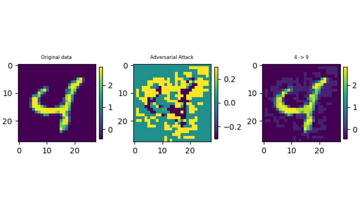
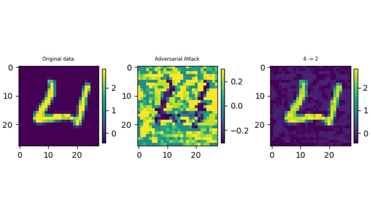
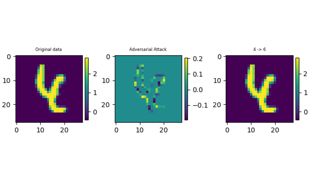
B.1 Visualization of Attacks
Adversarial attacks have to balance a trade-off between effectiveness (measured by decay in accuracy of the model) and detectability. Detectability is often quantified by a distance metric, but can be evaluated qualitatively - attacks that are successful but are not noticeable to the human eye are desireable, as this is the type of attack that poses the biggest threat in real-world applications. In Figure 9, we visualize natural and attacked images (along with their corresponding attacks) for FGSM, IFGSM, and CW attacks on MNIST of the naturally trained GLL model. Comparing the left and right-most columns, we see that FGSM and IFGSM models are easily detectable by the human eye, whereas the CW attacks are much more focused, and much less noticeable to the human eye. CW attacks are known to be much “smarter” than fast gradient methods (at the cost of more compute); GLL’s overall robustness to all three attacks is a strong result for our proposed model.
B.2 Replacing an MLP Classifier with GLL in Testing
Recall the MNIST setting from Section 4.3.3, where we used a “small CNN”. To further demonstrate the adversarial robustness of GLL, we replaced the final linear layer and softmax classifier used in the ”small CNN” with GLL during the attacks and testing and only during testing. That is, we trained in a normal fashion, before replacing the softmax classifier with GLL for either the attacking (that is, the attacks use the gradient information from GLL) and inference phases, or just for the inference phase. The results are presented in Figure 10. We see that - surprisingly - when we use the gradients from GLL for the attacks, the model is much more robust to FGSM. This supports the idea that GLL is more difficult to attack than the usual linear layer and softmax classifier.
B.3 Further CW Experiments
In Figure 8, we showed that for a fixed , GLL resists the adversary from moving the images compared to the softmax classifier. However, we also wanted to demonstrate that across distances in the CW attacks, GLL is also superior. To do so, we ran further experiments where we increased the value of so that the average distance increased further to the right. The results are shown in Figure 11. For MNIST, we ran additional experiments with . For CIFAR-10, we ran additional experiments with .
References
- Agrawal et al. (2019) Akshay Agrawal, Brandon Amos, Shane Barratt, Stephen Boyd, Steven Diamond, and J Zico Kolter. Differentiable convex optimization layers. Advances in neural information processing systems, 32, 2019.
- Barles and Souganidis (1991) Guy Barles and Panagiotis E Souganidis. Convergence of approximation schemes for fully nonlinear second order equations. Asymptotic analysis, 4(3):271–283, 1991.
- Belkin and Niyogi (2004) Mikhail Belkin and Partha Niyogi. Semi-supervised learning on Riemannian manifolds. Machine learning, 56:209–239, 2004.
- Belkin et al. (2004) Mikhail Belkin, Irina Matveeva, and Partha Niyogi. Regularization and semi-supervised learning on large graphs. In Learning Theory: 17th Annual Conference on Learning Theory, COLT 2004, Banff, Canada, July 1-4, 2004. Proceedings 17, pages 624–638. Springer, 2004.
- Bengio et al. (2006) Yoshua Bengio, Olivier Delalleau, and Nicolas Le Roux. Label Propagation and Quadratic Criterion, pages 193–216. MIT Press, semi-supervised learning edition, January 2006. URL https://www.microsoft.com/en-us/research/publication/label-propagation-and-quadratic-criterion/.
- Bertozzi and Flenner (2016) Andrea L Bertozzi and Arjuna Flenner. Diffuse interface models on graphs for classification of high dimensional data. SIAM Review, 58(2):293–328, 2016.
- Boyd et al. (2018) Zachary M. Boyd, Egil Bae, Xue-Cheng Tai, and Andrea L. Bertozzi. Simplified energy landscape for modularity using total variation. SIAM Journal on Applied Mathematics, 78(5):2439–2464, 2018. doi: 10.1137/17M1138972.
- Brown et al. (2023a) Jason Brown, Bohan Chen, Harris Hardiman-Mostow, Adrien Weihs, Andrea L Bertozzi, and Jocelyn Chanussot. Material identification in complex environments: Neural network approaches to hyperspectral image analysis. In 2023 13th Workshop on Hyperspectral Imaging and Signal Processing: Evolution in Remote Sensing (WHISPERS), pages 1–5. IEEE, 2023a.
- Brown et al. (2023b) Jason Brown, Riley O’Neill, Jeff Calder, and Andrea L Bertozzi. Utilizing contrastive learning for graph-based active learning of sar data. In Algorithms for Synthetic Aperture Radar Imagery XXX, volume 12520, pages 181–195. SPIE, 2023b.
- Calder (2018) Jeff Calder. The game theoretic p-Laplacian and semi-supervised learning with few labels. Nonlinearity, 32(1):301, 2018.
- Calder (2019) Jeff Calder. Consistency of Lipschitz learning with infinite unlabeled data and finite labeled data. SIAM J. on Mathematics of Data Science, 1(4):780–812, January 2019. doi: 10.1137/18m1199241.
- Calder and Drenska (2024) Jeff Calder and Nadejda Drenska. Consistency of semi-supervised learning, stochastic tug-of-war games, and the p-laplacian. To appear in Active Particles, Volume 4, Advances in Theory, Models, and Applications, 2024.
- Calder and Ettehad (2022) Jeff Calder and Mahmood Ettehad. Hamilton-jacobi equations on graphs with applications to semi-supervised learning and data depth. Journal of Machine Learning Research, 23(318):1–62, 2022.
- Calder and García Trillos (2022) Jeff Calder and N. García Trillos. Improved spectral convergence rates for graph Laplacians on -graphs and k-NN graphs. Applied and Computational Harmonic Analysis, 60:123–175, 2022. URL https://doi.org/10.1016/j.acha.2022.02.004.
- Calder and Slepcev (2020) Jeff Calder and Dejan Slepcev. Properly-weighted graph laplacian for semi-supervised learning. Applied Mathematics & Optimization, 82:1111–1159, 2020.
- Calder et al. (2020) Jeff Calder, Brendan Cook, Matthew Thorpe, and Dejan Slepcev. Poisson learning: Graph based semi-supervised learning at very low label rates. In International Conference on Machine Learning, pages 1306–1316. PMLR, 2020.
- Calder et al. (2023) Jeff Calder, Dejan Slepcev, and Matthew Thorpe. Rates of convergence for laplacian semi-supervised learning with low labeling rates. Research in the Mathematical Sciences, 10(1):10, 2023.
- Carlini and Wagner (2017) Nicholas Carlini and David Wagner. Towards evaluating the robustness of neural networks. In 2017 ieee symposium on security and privacy (sp), pages 39–57. Ieee, 2017.
- Chapman et al. (2023) James Chapman, Bohan Chen, Zheng Tan, Jeff Calder, Kevin Miller, and Andrea L Bertozzi. Novel batch active learning approach and its application to synthetic aperture radar datasets. In Algorithms for Synthetic Aperture Radar Imagery XXX, volume 12520, pages 95–110. SPIE, 2023.
- Chen et al. (2023a) Bohan Chen, Kevin Miller, Andrea L Bertozzi, and Jon Schwenk. Batch active learning for multispectral and hyperspectral image segmentation using similarity graphs. Communications on Applied Mathematics and Computation, pages 1–21, 2023a.
- Chen et al. (2023b) Bohan Chen, Kevin Miller, Andrea L. Bertozzi, and Jon Schwenk. Graph-based active learning for surface water and sediment detection in multispectral images. In IGARSS 2023 - 2023 IEEE International Geoscience and Remote Sensing Symposium, pages 5431–5434, 2023b. doi: 10.1109/IGARSS52108.2023.10282009.
- Chen et al. (2024) Bohan Chen, Kevin Miller, Andrea L Bertozzi, and Jon Schwenk. Batch active learning for multispectral and hyperspectral image segmentation using similarity graphs. Communications on Applied Mathematics and Computation, 6(2):1013–1033, 2024.
- Chen et al. (2020a) Ting Chen, Simon Kornblith, Mohammad Norouzi, and Geoffrey Hinton. A simple framework for contrastive learning of visual representations. In International conference on machine learning, pages 1597–1607. PMLR, 2020a.
- Chen et al. (2020b) Ting Chen, Simon Kornblith, Kevin Swersky, Mohammad Norouzi, and Geoffrey E Hinton. Big self-supervised models are strong semi-supervised learners. Advances in neural information processing systems, 33:22243–22255, 2020b.
- Cortes and Vapnik (1995) Corinna Cortes and Vladimir Vapnik. Support-vector networks. Machine Learning, 20(3):273–297, 1995.
- Defferrard et al. (2016) Michaël Defferrard, Xavier Bresson, and Pierre Vandergheynst. Convolutional neural networks on graphs with fast localized spectral filtering. Advances in neural information processing systems, 29, 2016.
- Dunlop et al. (2020) Matthew M Dunlop, Dejan Slepcev, Andrew M Stuart, and Matthew Thorpe. Large data and zero noise limits of graph-based semi-supervised learning algorithms. Applied and Computational Harmonic Analysis, 49(2):655–697, 2020.
- El Alaoui et al. (2016) Ahmed El Alaoui, Xiang Cheng, Aaditya Ramdas, Martin J Wainwright, and Michael I Jordan. Asymptotic behavior of -based laplacian regularization in semi-supervised learning. In Conference on Learning Theory, pages 879–906. PMLR, 2016.
- Enwright et al. (2023) Joshua Enwright, Harris Hardiman-Mostow, Jeff Calder, and Andrea Bertozzi. Deep semi-supervised label propagation for sar image classification. In Algorithms for Synthetic Aperture Radar Imagery XXX, volume 12520, pages 160–172. SPIE, 2023.
- Flores et al. (2022) Mauricio Flores, Jeff Calder, and Gilad Lerman. Analysis and algorithms for -based semi-supervised learning on graphs. Applied and Computational Harmonic Analysis, 60:77–122, 2022.
- Garcia-Cardona et al. (2014) Cristina Garcia-Cardona, Ekaterina Merkurjev, Andrea L Bertozzi, Arjuna Flenner, and Allon G Percus. Multiclass data segmentation using diffuse interface methods on graphs. IEEE transactions on pattern analysis and machine intelligence, 36(8):1600–1613, 2014.
- García Trillos et al. (2020) Nicolás García Trillos, Moritz Gerlach, Matthias Hein, and Dejan Slepcev. Error estimates for spectral convergence of the graph Laplacian on random geometric graphs toward the Laplace–Beltrami operator. Foundations of Computational Mathematics, 20(4):827–887, 2020.
- Goodfellow et al. (2016) Ian Goodfellow, Yoshua Bengio, and Aaron Courville. Deep Learning. MIT Press, Cambridge, MA, USA, 2016.
- Goodfellow et al. (2014) Ian J Goodfellow, Jonathon Shlens, and Christian Szegedy. Explaining and harnessing adversarial examples. arXiv preprint arXiv:1412.6572, 2014.
- Ham et al. (2005) Jihun Ham, Daniel Lee, and Lawrence Saul. Semisupervised alignment of manifolds. In International Workshop on Artificial Intelligence and Statistics, pages 120–127. PMLR, 2005.
- He et al. (2016a) Kaiming He, Xiangyu Zhang, Shaoqing Ren, and Jian Sun. Deep residual learning for image recognition. In Proceedings of the IEEE conference on computer vision and pattern recognition, pages 770–778, 2016a.
- He et al. (2016b) Kaiming He, Xiangyu Zhang, Shaoqing Ren, and Jian Sun. Identity mappings in deep residual networks. In Computer Vision–ECCV 2016: 14th European Conference, Amsterdam, The Netherlands, October 11–14, 2016, Proceedings, Part IV 14, pages 630–645. Springer, 2016b.
- Hein et al. (2005) Matthias Hein, Jean-Yves Audibert, and Ulrike Von Luxburg. From graphs to manifolds-weak and strong pointwise consistency of graph laplacians. In COLT, volume 3559, pages 470–485. Springer, 2005.
- Hein et al. (2007) Matthias Hein, Jean-Yves Audibert, and Ulrike von Luxburg. Graph Laplacians and their convergence on random neighborhood graphs. Journal of Machine Learning Research, 8(6), 2007.
- Ho (1995) Tin Kam Ho. Random decision forests. In Proceedings of 3rd International Conference on Document Analysis and Recognition, volume 1, pages 278–282. IEEE, 1995.
- Hochreiter (1998) Sepp Hochreiter. The vanishing gradient problem during learning recurrent neural nets and problem solutions. International Journal of Uncertainty, Fuzziness and Knowledge-Based Systems, 6(02):107–116, 1998.
- Hu et al. (2015) Huiyi Hu, Justin Sunu, and Andrea L. Bertozzi. Multi-class graph mumford-shah model for plume detection using the mbo scheme. In Springer Lecture Notes in Computer Science, volume 8932, pages 209–222, 2015.
- Iscen et al. (2019) Ahmet Iscen, Giorgos Tolias, Yannis Avrithis, and Ondrej Chum. Label propagation for deep semi-supervised learning. In Proceedings of the IEEE/CVF conference on computer vision and pattern recognition, pages 5070–5079, 2019.
- Khosla et al. (2020) Prannay Khosla, Piotr Teterwak, Chen Wang, Aaron Sarna, Yonglong Tian, Phillip Isola, Aaron Maschinot, Ce Liu, and Dilip Krishnan. Supervised contrastive learning. Advances in neural information processing systems, 33:18661–18673, 2020.
- Kingma and Ba (2014) Diederik P Kingma and Jimmy Ba. Adam: A method for stochastic optimization. arXiv preprint arXiv:1412.6980, 2014.
- Kingma and Welling (2013) Diederik P Kingma and Max Welling. Auto-encoding variational bayes. ArXiv Preprint ArXiv, 2013.
- Kipf and Welling (2016) Thomas N Kipf and Max Welling. Semi-supervised classification with graph convolutional networks. In International Conference on Learning Representations, 2016.
- Krizhevsky et al. (2009) Alex Krizhevsky, Geoffrey Hinton, et al. Learning multiple layers of features from tiny images. Toronto, ON, Canada, 2009.
- Kurakin et al. (2018) Alexey Kurakin, Ian J Goodfellow, and Samy Bengio. Adversarial examples in the physical world. In Artificial intelligence safety and security, pages 99–112. Chapman and Hall/CRC, 2018.
- LeCun et al. (1989) Yann LeCun, Bernhard Boser, John S Denker, Donnie Henderson, Richard E Howard, Wayne Hubbard, and Lawrence D Jackel. Backpropagation applied to handwritten zip code recognition. Neural Computation, 1(4):541–551, 1989.
- Lee et al. (2013) Wen-Yu Lee, Liang-Chi Hsieh, Guan-Long Wu, and Winston Hsu. Graph-based semi-supervised learning with multi-modality propagation for large-scale image datasets. Journal of visual communication and image representation, 24(3):295–302, 2013.
- Loshchilov and Hutter (2016) Ilya Loshchilov and Frank Hutter. Sgdr: Stochastic gradient descent with warm restarts. arXiv preprint arXiv:1608.03983, 2016.
- Lu et al. (2020) Lu Lu, Yeonjong Shin, Yanhui Su, and George Em Karniadakis. Dying relu and initialization: Theory and numerical examples. Communications in Computational Physics, 28(5):1671–1706, 2020. ISSN 1991-7120. doi: https://doi.org/10.4208/cicp.OA-2020-0165. URL http://global-sci.org/intro/article_detail/cicp/18393.html.
- Madry et al. (2017) Aleksander Madry, Aleksandar Makelov, Ludwig Schmidt, Dimitris Tsipras, and Adrian Vladu. Towards deep learning models resistant to adversarial attacks. arXiv preprint arXiv:1706.06083, 2017.
- Manfredi et al. (2015) Juan J Manfredi, Adam M Oberman, and Alexander P Sviridov. Nonlinear elliptic partial differential equations and p-harmonic functions on graphs. Differential Integral Equations, 28(1-2):79–102, 2015.
- Merkurjev et al. (2013) Ekaterina Merkurjev, Tijana Kostić, and Andrea L. Bertozzi. An mbo scheme on graphs for classification and image processing. SIAM Journal on Imaging Sciences, 6(4):1903–1930, January 2013. doi: 10.1137/120886935. URL https://epubs.siam.org/doi/abs/10.1137/120886935.
- Merkurjev et al. (2017) Ekaterina Merkurjev, Andrea Bertozzi, Xiaoran Yan, and Kristina Lerman. Modified cheeger and ratio cut methods using the ginzburg–landau functional for classification of high-dimensional data. Inverse Problems, 33(7):074003, 2017.
- Merkurjev et al. (2018) Ekaterina Merkurjev, Andrea L Bertozzi, and Fan Chung. A semi-supervised heat kernel pagerank mbo algorithm for data classification. Communications in mathematical sciences, 16(5):1241–1265, 2018.
- Miller and Calder (2023) Kevin Miller and Jeff Calder. Poisson reweighted laplacian uncertainty sampling for graph-based active learning. SIAM Journal on Mathematics of Data Science, 5(4):1160–1190, 2023.
- Miller et al. (2022) Kevin Miller, Jack Mauro, Jason Setiadi, Xoaquin Baca, Zhan Shi, Jeff Calder, and Andrea L Bertozzi. Graph-based active learning for semi-supervised classification of sar data. In Algorithms for Synthetic Aperture Radar Imagery XXIX, volume 12095, pages 126–139. SPIE, 2022.
- Miller and Bertozzi (2024) Kevin S Miller and Andrea L Bertozzi. Model change active learning in graph-based semi-supervised learning. Communications on Applied Mathematics and Computation, pages 1–29, 2024.
- Montufar et al. (2014) Guido F Montufar, Razvan Pascanu, Kyunghyun Cho, and Yoshua Bengio. On the number of linear regions of deep neural networks. Advances in neural information processing systems, 27, 2014.
- Nadler et al. (2009) Boaz Nadler, Nathan Srebro, and Xueyuan Zhou. Semi-supervised learning with the graph Laplacian: The limit of infinite unlabelled data. In Proceedings of the 22nd International Conference on Neural Information Processing Systems, NIPS’09, page 1330–1338, Red Hook, NY, USA, 2009. Curran Associates Inc. ISBN 9781615679119.
- Pedregosa et al. (2011) F. Pedregosa, G. Varoquaux, A. Gramfort, V. Michel, B. Thirion, O. Grisel, M. Blondel, P. Prettenhofer, R. Weiss, V. Dubourg, J. Vanderplas, A. Passos, D. Cournapeau, M. Brucher, M. Perrot, and E. Duchesnay. Scikit-learn: Machine learning in Python. Journal of Machine Learning Research, 12:2825–2830, 2011.
- Pu et al. (2016) Yunchen Pu, Zhe Gan, Ricardo Henao, Xin Yuan, Chunyuan Li, Andrew Stevens, and Lawrence Carin. Variational autoencoder for deep learning of images, labels and captions. Advances in Neural Information Processing Systems, 29, 2016.
- Sellars et al. (2021) Philip Sellars, Angelica I Aviles-Rivero, and Carola-Bibiane Schönlieb. Laplacenet: A hybrid energy-neural model for deep semi-supervised classification. arXiv preprint arXiv:2106.04527, 2021.
- Settles (2009) Burr Settles. Active learning literature survey. University of Wisconsin-Madison Department of Computer Sciences, 2009.
- Shi et al. (2017) Zuoqiang Shi, Stanley Osher, and Wei Zhu. Weighted nonlocal laplacian on interpolation from sparse data. Journal of Scientific Computing, 73:1164–1177, 2017.
- Slepcev and Thorpe (2019) Dejan Slepcev and Matthew Thorpe. Analysis of p-Laplacian regularization in semisupervised learning. SIAM Journal on Mathematical Analysis, 51(3):2085–2120, 2019.
- Szegedy et al. (2013) Christian Szegedy, Wojciech Zaremba, Ilya Sutskever, Joan Bruna, Dumitru Erhan, Ian Goodfellow, and Rob Fergus. Intriguing properties of neural networks. arXiv preprint arXiv:1312.6199, 2013.
- Velicković et al. (2017) Petar Velicković, Guillem Cucurull, Arantxa Casanova, Adriana Romero, Pietro Lio, and Yoshua Bengio. Graph attention networks. arXiv preprint arXiv:1710.10903, 2017.
- Von Luxburg (2007) Ulrike Von Luxburg. A tutorial on spectral clustering. Statistics and computing, 17:395–416, 2007.
- Wang and Osher (2021) Bao Wang and Stan J Osher. Graph interpolating activation improves both natural and robust accuracies in data-efficient deep learning. European Journal of Applied Mathematics, 32(3):540–569, 2021.
- Wang et al. (2013) Bo Wang, Zhuowen Tu, and John K Tsotsos. Dynamic label propagation for semi-supervised multi-class multi-label classification. In Proceedings of the IEEE international conference on computer vision, pages 425–432, 2013.
- Wang et al. (2023) Yifei Wang, Qi Zhang, Tianqi Du, Jiansheng Yang, Zhouchen Lin, and Yisen Wang. A message passing perspective on learning dynamics of contrastive learning. In International Conference on Learning Representations, 2023.
- Wu et al. (2020) Zonghan Wu, Shirui Pan, Fengwen Chen, Guodong Long, Chengqi Zhang, and S Yu Philip. A comprehensive survey on graph neural networks. IEEE transactions on neural networks and learning systems, 32(1):4–24, 2020.
- Xiao et al. (2017) Han Xiao, Kashif Rasul, and Roland Vollgraf. Fashion-mnist: a novel image dataset for benchmarking machine learning algorithms. arXiv preprint arXiv:1708.07747, 2017.
- Yann LeCun (2010) Christopher J.C. Burges Yann LeCun, Corinna Cortes. Mnist handwritten digit database. http://yann.lecun.com/exdb/mnist/, 2010.
- Zhou and Belkin (2011) Xueyuan Zhou and Mikhail Belkin. Semi-supervised learning by higher order regularization. In Proceedings of the Fourteenth International Conference on Artificial Intelligence and Statistics, pages 892–900. JMLR Workshop and Conference Proceedings, 2011.
- Zhu et al. (2003) Xiaojin Zhu, Zoubin Ghahramani, and John D Lafferty. Semi-supervised learning using gaussian fields and harmonic functions. In Proceedings of the 20th International conference on Machine learning (ICML-03), pages 912–919, 2003.