FLRONet: Deep Operator Learning for High-Fidelity Fluid Flow Field Reconstruction from Sparse Sensor Measurements

Abstract

The ability to reconstruct high-fidelity fluid flow fields from sparse sensor measurement is critical for many science and engineering applications, but remains a huge challenge. This challenge is caused by the large difference between the dimensions of the state space and the observational space, making the operator that provides the mapping from the state space to the observational space ill-conditioned and non-invertible. As a result, deriving the forward map from the observational space to the state space as the inverse of the measurement operator is nearly impossible. While traditional methods, including sparse optimization, data assimilation, or machine learning based regressive reconstruction, are available, they often struggle with generalization and computational efficiency, particularly when non-uniform or varying discretization of the domain are considered. In this work, we propose FLRONet, a novel operator learning framework designed to reconstruct full-state flow fields from sparse sensor measurements in space and time. FLRONet utilizes a branch-trunk architecture, where the branch network integrates sensor observations from multiple time instances, and the trunk network encodes the entire temporal domain. This design allows FLRONet to achieve highly accurate, discretization-independent reconstructions at any time within the observation window. Although the popular three-dimensional Fourier Neural Operator offers similar functionalities, our results show that FLRONet surpasses it in both accuracy and efficiency. FLRONet not only achieves superior performance in approximating the true operator but also exhibits significantly faster inference at high-fidelity discretizations.

I Introduction

The ability to reconstruct the fluid flow field from limited sensor measurements is crucial for numerous science and engineering applications. In this problem, the objective is to reconstruct the high-fidelity flow field, denoted as $\mathbf{u}(t)\in\mathbb{R}^{m}$, from a limited number of sensor observations $\mathbf{y}(t)\in\mathbb{R}^{p}$. This task is inherently challenging due to the unique properties of the measurement operator $\mathcal{H}:\mathbb{R}^{m}\to\mathbb{R}^{p}$ that maps a given state of the flow field $\mathbf{u}(t)$ to the corresponding sensor observations $\mathbf{y}(t)$ given a set of sensors located within the domain of interest. Since the dimension of the observational space, $p$, is typically much smaller than the dimension of the state space, $m$, the measurement operator is often ill-conditioned and non-invertible. As a result, obtaining the forward map, $\mathcal{G}:\mathbb{R}^{p}\to\mathbb{R}^{m}$, as the inverse of $\mathcal{H}$ is nearly impossible. Instead, alternative strategies such as data-driven approaches Erichson et al. (2020), sparse optimization Loiseau, Noack, and Brunton (2018), and data assimilation Mons et al. (2016) are often employed. Despite significant progress reported in the literature, reconstructing full-state flow fields from sparse measurements remains a challenging and unresolved issue.

The emergence of machine learning, particularly deep learning, has significantly advanced the research on flow field reconstruction with sparse sensor measurements. Powered by the strong modeling capability of neural networks, deep learning models trained with computational fluid dynamic (CFD) simulation data have been widely employed for field reconstruction. Specifically, deep learning plays a significant role in various stages of the field reconstruction process. For instance, deep learning can be used to directly learn the inverse operator, as demonstrated in Erichson et al. Erichson et al. (2020), Wu et al. Wu, Xiao, and Luo (2023), or Li et al. Li et al. (2024). In addition, it can be used to provide an efficient representation scheme, also known as the implicit neural representation, which, later, can be used to facilitate the sparse optimization for field reconstruction. Finally, deep learning can also contribute to the data assimilation approach by serving as a prior regression from sensor observations or as a dynamic model for rough predictions Cheng et al. (2024).

The literature has reported that deep learning-based reconstructions often yield higher accuracy and are significantly faster than traditional methods based on modal decomposition or direct numerical simulation. However, despite these successes, recent advancements in deep learning for flow field reconstruction are limited in their ability to generalize across different discretization schemes since they mostly focus on learning the map between vector spaces. This poses a significant limitation in practice, where non-uniform or varying mesh systems are commonly encountered, preventing the widespread application of deep learning for flow field reconstruction from sensor measurement.

For this reason, efforts have shifted toward operator learning, which operates on functional spaces instead of vector spaces, as in the case of neural networks. For instance, neural operators Kovachki et al. (2023), an approximation paradigm that operates on functional spaces, have been proposed recently. Notably, neural operators offer discretization-invariant capabilities, meaning they are independent of the chosen mesh system and can achieve zero-shot super-resolution. This is a significant advantage, as engineering data are often provided in non-uniform grid systems that vary depending on the geometry of the domain. Moreover, experimental studies demonstrate that neural operators, with their inductive bias architectures, outperform other deep learning methods in approximating partial differential equation (PDE) solutions and can replace CFD simulations due to their computational efficiency after training. Inspired by the above advantages of neural operators, Zhao et al. Zhao et al. (2024) proposed RecFNO, a model based on the Fourier Neural Operator (FNO) Li et al. (2020), for the reconstruction of heat flow fields from sparse sensor measurements. The authors have demonstrated an enhanced reconstruction capability for RecFNO compared to other deep learning methods. Moreover, with the zero-shot super-resolution capability, RecFNO can achieve up to eight times the resolution refinement without retraining. However, while RecFNO’s discretization-independent capability is demonstrated in the spatial domain, this is not guaranteed in the temporal domain. Although 3D FNO models could be applied, their computational efficiency and effectiveness remain in question, as their ineffectiveness in the temporal domain has been consistently demonstrated in several other applications Nguyen et al. (2024).

Deep Operator Network (DeepONet) Lu et al. (2021) is another powerful approximation scheme that has been proven to be highly effective for operator learning. Building on the universal approximation theorem of deep neural networks, Lu et al. Lu et al. (2021) extended this concept to enable the learning of continuous operators and complex systems from scattered data streams. DeepONet is made up of two networks: the branch network and the trunk network. In DeepONet, the branch net encodes the input function given in the discrete setting, while the trunk net encodes the domain of the output functions. The outputs of these two networks are seamlessly combined through element-wise multiplication, which resembles the Green’s function. Since its introduction, DeepONet has been widely used for various applications in the physics domain and has demonstrated great success. Moreover, DeepONet also provides an ability to learn the operator that operate on both space time domains with high efficiency as will be demonstrated later.

In this work, we utilize DeepONet to reconstruct the flow field from limited sensor measurements. Given the sensor observation at specific locations in space-time domains, our goal is to reconstruct the full-state flow fields at a given time within the observation time window. To achieve this goal, we propose FLRONet, a deep operator network that can reconstruct the full state flow field at any given time within the input time window and is independent of the discretization scheme in the spatial domain, based on limited sensor observations. FLRONet also consists of two networks: branch net and trunk net. For the branch net, we utilized FNO to combine sensor observations from various time stamps. For trunk net, we employed an MLP to encode the time domain of the output. Similar to DeepONet, the outputs of the branch net and trunk net are combined to derive the final reconstruction of the full-state flow field at a given time within the observational window.

II Problem formulation

Given a fluid flow system in which the state of the flow field can be described as a function of time $\mathbf{u}(t)$ that returns value in $\mathbb{R}^{m}$. At discrete time points $\tau_{i}\in\left[\tau_{0},\tau_{1},...,\tau_{n}\right]$, the measurement $\mathbf{y}\in\mathbb{R}^{p}$ are obtained at $p$ locations over the state field via the measurement operator $\mathcal{H}:\mathbb{R}^{m}\to\mathbb{R}^{p}$:

$$\mathbf{y}=\mathcal{H}[\mathbf{u}].$$

Here, our goal is, to reconstruct the state field $\mathbf{u}$ from the sparse observation $\mathbf{y}$ for a for a given time $t\in[\tau_{0},\tau_{n}]$. Essentially, this task is equivalent to finding the forward operator $\mathcal{G}:\mathbb{R}^{p}\to\mathbb{R}^{m}$ that is, in theory, the inverse of the measurement operator $\mathcal{H}:\mathbb{R}^{m}\to\mathbb{R}^{p}$:

$$\mathbf{u}=\mathcal{G}[\mathbf{y}]\approx\mathcal{H}^{-1}[\mathbf{y}].$$

However, unlike existing methods which target to model $\mathcal{G}$ as a map between the sensor observation and the state field for a single discrete time point, we want to incorporate the dynamic characteristic of the fluid flow which add an addition constraint to the learning process to guarantee the integrity of the reconstructed field. Moreover, we also want our reconstructed field to be independent from the selected discretization settings. As a result, our objectives is transformed to reconstructing the state field $\mathbf{u}$ given a set of sensor observations at discrete time points $\left[\mathbf{y}(\tau_{0}),\mathbf{y}(\tau_{1}),...,\mathbf{y}(\tau_{n})\right]$ for any given time $t\in\left[\tau_{0},\tau_{n}\right]$:

$$\mathbf{u}(t)=\mathcal{G}[\mathbf{y}(\tau_{1}),\mathbf{y}(\tau_{2}),...,\mathbf{y}(\tau_{n})](t).$$

with $\mathbf{u}$ is discretization independent. With the above formulation and inspired by the deep operator theory by Lu et al. Lu et al. (2021), we approximate the operator $\mathcal{G}$ by a deep operator network for which we named FLRONet.

III Methodology

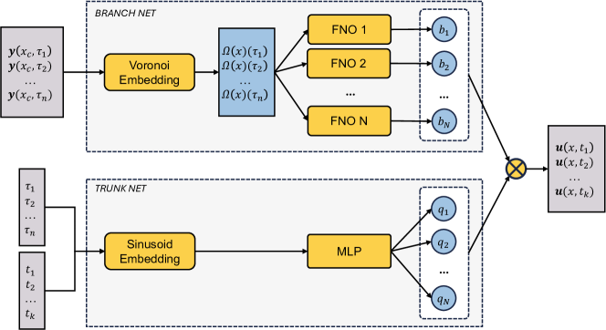
Figure 1: FLRONet with 2-dimensional Fourier Neural Operators as the unstacked branch net and MLP as the trunk net.

III.1 Architecture design

As illustrated in Fig. 1, FLRONet contains two networks: branch net and trunk net. As similar to DeepONet, branch net is responsible for encoding the information at discrete sampling location, in this case, the sensor observation at recorded time points. Meanwhile, the trunk net is responsible for encoding the output domain, which is in this case, the time domain for the state field. In more particular, the branch net take the sensor observation at $n$ discrete time points $\{\tau_{0},\tau_{1},...,\tau_{n}\}$ and produced $N$ output fields using $N$ unstacked branch nets. Here we use Fourier Neural Operator Li et al. (2020) to model the unstacked branch net to enable the spatial discretization independent capability. For sensor observation, we used the Voronoi embedding, which will be discussed in detail in Subsection III.3, to encapsulate the position on both the value of the sensor and the position of the sensor. For the trunk net, the reconstruction time vector $\mathbf{t}\in\mathbb{R}^{k}$ along with the sensory time vector $\bm{\tau}\in\mathbb{R}^{n}$ are sent through a sinusoid embedding before processed by an MLP network that consists of 3 layers to produced the $N$ output value. In this particular problem, we choose $N=2$, $k=1$ and $n=5$. The output of branch net and the trunk net is combined using dot product to make the final prediction on the reconstructed flow field.

III.2 Operator network for spatiotemporal discretization independent

DeepONet with FNO branch net

We employ the DeepONet to achieve the temporal resolution independent. Using DeepONet, the forward operator $\mathcal{G}$ can be modeled as follow:

$$\mathcal{G}(\mathbf{y}(\bm{\tau}))(\mathbf{t})=\mathcal{B}(\mathbf{y}(\bm{\tau}))\otimes\mathcal{T}(\mathbf{t}|\bm{\tau}).$$ (1)

In Eq. 1, the branch network $\mathcal{B}$ processes sensor measurements $\mathbf{y}$ at sensory time instances $\bm{\tau}$, and the trunk network $\mathcal{T}$ takes as input the reconstruction time points $\mathbf{t}$, which are conditioned on $\bm{\tau}$, to capture the relative proximity between $\mathbf{t}$ and $\bm{\tau}$. Lastly, the fusing operation is denoted as $\otimes$.

The trunk network $\mathcal{T}$ is modeled using an MLP with three fully connected layers, preceded by a sinusoidal embedding, denoted as $\Phi$, to enhance the representation of relative temporal positions. The sinusoidal embeddings of the sensory time instances $\bm{\tau}$ and the reconstruction time points $\mathbf{t}$ are combined using a dot product, where the dot product value increases in response to the temporal proximity. This design allows the trunk network to effectively capture the temporal relationship between sensory inputs and reconstruction targets.

The branch network $\mathcal{B}$ follows the unstacked version of DeepONet Lu et al. (2021) to increase the expressive power of FLRONet. Although the branch network can be implemented using a variety of architectures, including U-Net Ronneberger, Fischer, and Brox (2015) and fully connected networks Lu et al. (2021), we utilize the FNO in this study to accomplish the spatial resolution invariance. A Voronoi embedding, denoted as $\Omega$, is implemented prior to the FNO blocks in order to encode sensor measurements. The fusing operation is simply performed as a dot product $\langle\cdot,\cdot\rangle$, leading to the explicit formulation of Eq. 1 as follows:

$$\mathcal{G}(\mathbf{y}(\bm{\tau}))(\mathbf{t})=\langle\text{FNO}(\Omega(\mathbf{y})),\text{MLP}(\Phi(\mathbf{t})\cdot\Phi(\bm{\tau})\rangle.$$ (2)

FNO branch net

In this study, we employed 2-dimensional FNO to model the branch net to achieve the spatial resolution independent capability. At each sensory time point $\tau_{i}$, the input to an FNO branch is the corresponding sensor measurement after processed by the Voronoi embedding layer which can be considered as a function of space $\Omega(\mathbf{x})$. The FNO in Eq. 2 can be defined as:

$$\text{FNO}(\Omega(x))=\mathcal{F}^{-1}(\mathcal{F}(\kappa)\cdot\mathcal{F}(\Omega))(x),$$ (3)

where $\kappa$ is the the kernel function while $\mathcal{F}$ and $\mathcal{F}^{-1}$ are the Fourier transform and its inverse on the the spatial domain. By definition, for any function $f$ defined on the spatial domain $D$, the Fourier transform and its inverse are given as:

$$(\mathcal{F}f)(k)=\int_{D}f(x)e^{-2\pi ikx}\,dx,\quad(\mathcal{F}^{-1}f)(x)=\int_{D}\mathcal{F}(f)(k)e^{2\pi ikx}\,dk.$$ (4)

Considering that we are constrained to evaluating the value $\mathbf{u}(x)$ on a finite mesh. Equations 4 can be discretized by two-dimensional Discrete Fourier Transform (DFT) and Inverse Discrete Fourier Transform (IDFT). Assume that the examined domain is discretized into a uniform grid, where $N_{h}$ and $N_{w}$ are the number of grid points in the vertical and horizontal dimensions, respectively. The two-dimensional DFT and its inverse IDFT for a function $f$ defined on this grid are given by:

$$\text{DFT}(f)(k_{h},k_{w})=\sum_{n_{h}=0}^{N_{h}-1}\sum_{n_{w}=0}^{N_{w}-1}f(n_{h}\Delta h,n_{w}\Delta w)e^{-2\pi i\left(\frac{k_{h}n_{h}}{N_{h}}+\frac{k_{w}n_{w}}{N_{w}}\right)},\quad\text{IDFT}(f)(h,w)=\frac{1}{N_{h}N_{w}}\sum_{k_{h}=0}^{N_{h}-1}\sum_{k_{w}=0}^{N_{w}-1}f(k_{h},k_{w})e^{2\pi i\left(\frac{k_{h}n_{h}}{N_{h}}+\frac{k_{w}n_{w}}{N_{w}}\right)}.$$

Moreover, we adhere to the original parametrization for $\mathcal{F}(\kappa)$: Given $d$ as the embedding dimension, then $\mathcal{F}(\kappa)=R_{\phi}\in\mathbb{C}^{k_{h}\times k_{w}\times d\times d}$. Up to this point, we complete the definition of all components in Eq. 3.

Lastly, one of the main principles of the FNO is that it retains only the low-frequency modes for further processing, while truncating the rest. This principle is is based on Parseval’s Theorem, which indicates that the low-frequency modes of a function contain the majority of its information whereas high-frequency modes typically contain redundant details or noise. In this study, we choose $d=64$; and over the spatial domain of ($H\times W)=(140\times 240$), we retain upto $24$ modes along the vertical dimension ($k_{h}=24$) and $48$ modes along the horizontal dimension ($k_{w}=48$).

III.3 Voronoi tessellation assisted for sensor measurements embedding

Traditional regressive field reconstruction methods often represent sensor measurements as vectors Erichson et al. (2020); Dubois et al. (2022), which constrains the ability of machine learning models to generalize effectively toward different sensor settings (e.g., varying sensor locations or layouts). This representation scheme omits information about the sensor positions, leaving ML models unaware of the sensor locations and causing them to struggle with adapting to different sensor configurations Cheng et al. (2024). Several pioneer studies have attempted to apply masked images as a way to encode the sensor positions; however, these approaches cannot achieve proper reconstruction accuracy, especially when sensor measurements are sparse. In this work, we used Voronoi tessellation, which was inspired by Cheng et al. (2024)], to encode the information about sensor positions.

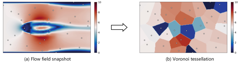
Figure 2: Voronoi-Tessellation-Based Embedding Method: (a) An original snapshot of the flow field from the CFD dataset, with 32 randomly distributed sensors marked as white dots. (b) The corresponding Voronoi tessellation, computed from sensor locations and field values.

Fig. 2 illustrates the Voronoi-tessellation-based embedding method. Given $n$ sensors located at positions with coordinates $\mathbf{x}_{ci}$ in the examined domain $D$, the Voronoi tessellation partitions $D$ into $n$ Voronoi cells, denoted as $V=[V_{1},V_{2},...V_{n}]$. Each Voronoi cell $V_{i}$ can be defined as:

$$V_{i}=\{\mathbf{x}\in D\mid d(\mathbf{x},\mathbf{x}_{ci})<d(\mathbf{x},\mathbf{x}_{cj}),\,\forall j\neq i\},$$ (5)

where $\mathbf{x}$ is a grid point in $V_{i}$, and $d(\cdot,\cdot)$ denotes the Euclidean distance between two points. After the Voronoi tessellation process, all grid points within each Voronoi cell are assigned the value of the sensor associated with that cell. This results in an embedding field with dimensions similar to those of the state field, which is later used as the input for FLRONet.

The defining feature of Voronoi tessellation-based embedding is that each Voronoi cell is influenced exclusively by its assigned sensor. This assigned sensor determines the values of all grid points within the cell. Moreover, the shape and size of each Voronoi cell are already optimized for its corresponding sensor; therefore, the influence of sensor observations on the value of a particular grid point is properly modeled. Another advantage of applying Voronoi tessellation-based embedding is that it allows the network to easily cope with different sensor configurations (e.g., varying sensor positions or the number of sensors used) without having to modify the architecture of the neural network. This advantage will be demonstrated later in Section IV.2 when FLRONet has to deal with missing sensor observations.

III.4 Data and Training

We trained FLRONet using the CFDBench cylinder dataset Yining, Yingfa, and Zhen (2023). The dataset contains numerical simulations of fluid flow around a cylindrical obstacle (Fig. 3). The examined domain has the physical size of $0.14\times 0.24(m)$, which is tessellated into a $140\times 240$ (pixels) grid. There are 50 simulation cases in the dataset, each having a unique inlet velocity increasing incrementally from 0.1 m/s to 5.0 m/s. For each simulation case, the total 1-second simulation time is recorded using 1,000 snapshots with the time interval between snapshots being 0.001 (s). For each case, 32 sensors are randomly distributed across the domain to record velocity magnitudes at 32 different locations, providing sparse observations that FLRONet uses as input. Fig. 3 illustrates the dimensions of the examined domain and the sensor layout.

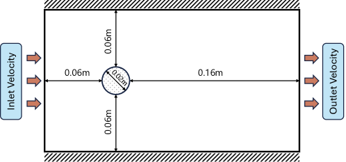
Figure 3: The geometry of the fluid flow around the circular cylinder problem as described in the CFD dataset.

To construct the training data, we create observation windows containing five snapshots of sensor data, with the time interval between two snapshots being 0.005 (s), resulting in a 0.02-second window. With this setup, 980 observation windows per case were generated. Within each window, we randomly select a single snapshot to record the velocity field at that time point, which serves as the ground truth for FLRONet’s predictions. To evaluate generalization, we randomly sampled the 50 simulation cases into two exclusive sets: 45 cases for training and five cases for testing. The training set includes all cases of inlet velocity, except for those specifically reserved for the test set. The test set consists of cases with inlet velocities of 3.5, 3.9, 4.2, 4.6, and 5.0 m/s. FLRONet was trained end-to-end using the Adam optimizer with a learning rate of $10^{-3}$, allowing the model to effectively learn the complex mappings from sparse sensor data to the full flow field.

III.5 Validation metrics

For quantitative validation of FLRONet, we used two metrics namely root mean squared error (RMSE) and mean absolute error (MAE). Given $T$ as the temporal resolution; particularly, the CFD dataset has $T=1,000$ (time steps). Denote $\hat{\mathbf{u}}(t)$ as the reconstructed field at time $t$, $\mathbf{u}(t)$ is the corresponding ground truth. The computation of these metrics is defined as follows:

$$\text{RMSE}=\frac{1}{T}\sum_{t=1}^{T}{\|\hat{\mathbf{u}}(t)-\mathbf{u}(t)\|_{2}},\quad\text{MAE}=\frac{1}{T}\sum_{t=1}^{T}{\|\hat{\mathbf{u}}(t)-\mathbf{u}(t)\|_{1}},$$ (6)

where $\|.\|_{2}$ and $\|.\|_{1}$ denote the $\ell_{2}$-norm and $\ell_{1}$-norm, respectively, computed over the spatial domain of the flow field at reconstruction time $t$.

IV Results and discussion

We validate our FLRONet on the CFDBench dataset described in Section III.4. For the benchmarking purpose, we compared the reconstruction capability of FLRONet with that of FNO 3D. We also included two additional branch net architectures for FLRONet, namely U-Net (FLRONet-UNet) and MLP (FLRONet-MLP), for comparison purposes. Here, we aim to demonstrate the unique ability of FLRONet with the FNO branch net (FLRONet-FNO) to perform zero-shot super-resolution in both space and time while still exhibiting high reconstruction accuracy compared to other baselines.

IV.1 Prediction accuracy

We first validate FLRONet in an ideal condition where all the sensor measurements are clean and free of noise. We also assume that FLRONet has data from all sensor observations for reconstruction. Based on this clean and perfect input, we ask FLRONet and other baselines to reconstruct the flow field at the exact time when the sensor data are measured. Fig. 4 shows the reconstructed flow fields, the ground truth from CFD, and the corresponding MAE maps for FLRONet-FNO and other baselines in the case where the inlet velocity is $3.5$ m/s, which is not included in the training. Visually, all baselines appear to be able to capture the overall structure of the flow field. Nonetheless, it is clear that FLRONet-FNO produces the most accurate reconstructions among all baselines. Its reconstruction fields are closely aligned with the ground truth fields from CFD. In contrast, FNO-3D, the primary competitor of FLRONet-FNO, exhibits significantly noisier reconstructions, particularly at the tail of the vortex shredding feature. Fig. 4 also suggests that the two other FLRONet baselines, FLRONet-MLP and FLRONet-UNet, offer the similar reconstruction capabilities as FLRONet-FNO. Their reconstructed fields are visually indistinguishable from those produced by FLRONet-FNO. However, as will be shown in the quantitative analysis, they actually exhibit slightly higher RMSE and MAE values.

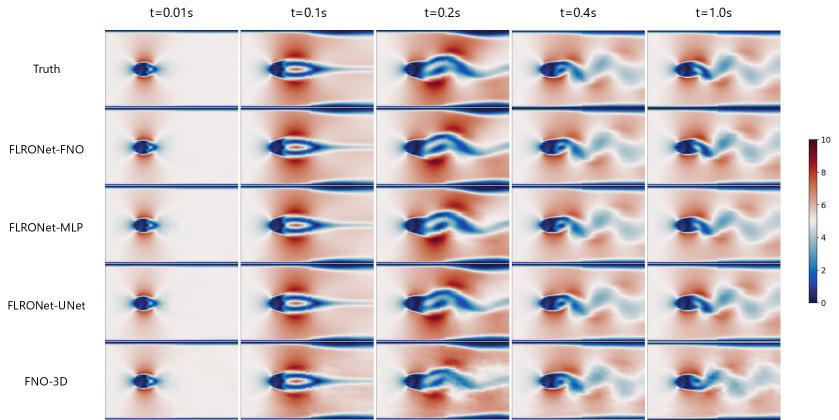
Figure 4: Reconstructed fluid flow across architectures for the boundary condition $v_{0}=3.5$ m/s: The comparison highlights differences in reconstruction quality, with FLRONet-FNO showing the closest resemblance to the ground truth.

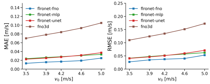
Figure 5: Average reconstruction error across unseen inlet velocities: FLRONet-FNO consistently achieves the lowest error. FLRONet-MLP and FLRONet-UNet perform similarly, with slightly higher errors compared to FLRONet-FNO. FNO-3D shows the highest errors, particularly at higher $v_{0}$.

The quantitative analysis presented in Fig. 5 has further confirmed the above qualitative observation. Specifically, in this experiment, we measure the average MAE and RMSE of the field reconstructed by FLRONet across all time steps in the simulation for all five tested inlet velocities ($v_{0}$), including $v_{0}=3.5,3.9,4.2,4.6,$ and $5.0$ m/s. As indicated in Fig. 5, the field reconstructed by FLRONet-FNO is consistently the most accurate, having the lowest reconstructed MAE and RMSE for all inlet velocities. Meanwhile, FLRONet-UNet and FLRONet-MLP exhibit moderately lower performance compared to FLRONet-FNO; nevertheless, all models in the FLRONet family exhibit much higher reconstruction accuracy when compared to FNO-3D. This result also serves as evidence of the FLRONet architecture’s greater suitability for the field reconstruction task compared to other operator learning methods like FNO-3D. One important observation we should point out is that the reconstruction accuracy of all models tends to increase as the inlet velocity increases. These results highlight the inherent difficulty of reconstructing flow with a high Reynolds number driven by the increased velocity of the fluid, which is characterized by more chaotic, multi-scale behaviors of flows. Despite these challenges, FLRONet-FNO still performs consistently and provides the most accurate reconstructed field from sparse sensor measurements.

The above validation results have demonstrated the ability of FLRONet to accurately reconstruct both large-scale flow features and finer flow structures under various boundary conditions. In the next sections, we will continue to validate FLRONet’s reconstruction capability given the imperfect conditions, including sensor loss or noisy measurement data. We will also explore the ability of FLRONet-FNO and FNO-3D to perform zero-shot super-resolution in both spatial and temporal domains.

IV.2 Robustness to incomplete sensor measurements

In practice, it is not always possible to acquire all the sensor data due to connection loss or sensor malfunction, forcing the machine learning model to reconstruct the flow field from incomplete sensor observations. In such scenarios, the consistency in the reconstruction accuracy of the model is critical and can affect downstream tasks. Therefore, it is important to assure the consistent performance of FLRONet in case of incomplete sensor measurement. In this experiment, we evaluate the reconstruction accuracy of FLRONet-FNO and other baselines in the case of missing one or several sensor observations. We randomly remove one or a few sensors and measure the reconstruction accuracy of all baselines when they are reconstructed from the remaining subset of sensors. Particularly, we iteratively remove up to 20 random sensors from the original 32 and compare the RMSE and MAE of all baselines.

Figure 6 shows the performance of the FLONet with different branch nets and FNO-3D in the case of missing sensor observations. The result in Fig. 6 demonstrates a strong resilience to missing sensor data from FLRONet-FNO, FLRONet-UNet, and FNO-3D, while FLRONet-MLP is exceedingly sensitive to missing sensory inputs. As indicated in Fig. 6, FLRONet-MLP experiences an exponential increase in both RMSE and MAE values as the number of missing sensors increases. In contrast, FLRONet-FNO, FLRONet-UNet, and FNO-3D all maintain robust reconstruction accuracy. Interestingly, all of these models leverage the Voronoi embedding layer to encode input sensor data, which likely contributes to their consistent accuracy under incomplete sensor measurements. From the sensor coordinates, the Voronoi embedding layer effectively encodes the spatial relationships among sensors. It allows the missing values to be easily interpolated back from their nearest neighbors. This interpolation mechanism plays as a buffer to withstand the degradation of input quality caused by missing data. Conversely, in the case of FLRONet-MLP, there is no mechanisms to incorporate any spatial information from the sensors; therefore, when some sensors are lost, their values are unavoidably dropped to zeros, which severely distorts the reconstruction results.

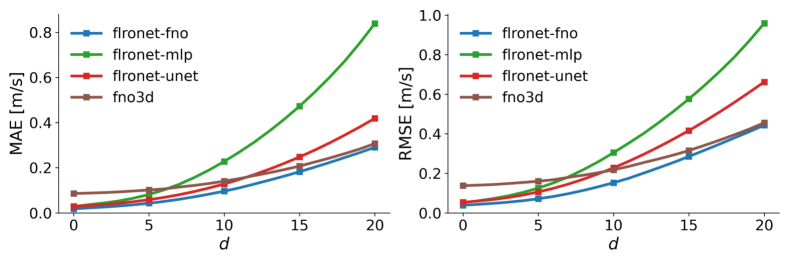
Figure 6: Reconstruction performance under different numbers of lost sensors: The figure shows the MAE and RMSE of FLRONet-based models and FNO-3D as the number of lost sensors, $d$, increases from 0 to 20. FLRONet-FNO and FNO-3D handle sensor loss effectively, showing minimal error increase. FLRONet-UNet performs well for small $d$ but degrades gradually as $d>5$. FLRONet-MLP delivers the poorest performance, with a steep error increase due to its lack of spatial interpolation capabilities.

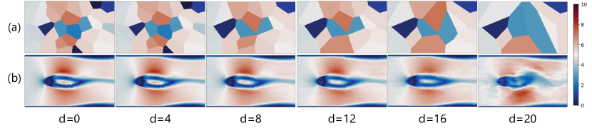
Figure 7: Reconstruction performance with missing sensors: The number of missing sensors, $d$ ranges from 0 to 20 out of a total of 32. Row (a) displays the resulting Voronoi input at each level of sensor loss. Row (b) presents the corresponding reconstructed velocity field.

In addition to the Voronoi embedding’s advantage, Fourier-based methods like FNO-3D and FLRONet-FNO tend to exhibit slower accuracy degradation, making them more resilient to sensor loss. This resilience stems from the fundamental property of Fourier-based approaches, which aim to learn an operator mapping between two functional spaces. These methods treat input data as a continuous function, enabling missing values to be interpolated naturally through the function’s continuity before being fed to the operator. As a result, the distance between the complete sensor input function $\mathbf{y}(t)$ and the incomplete sensor input function $\mathbf{y^{\prime}}(t)$ remains small.

Next, we qualitatively evaluate the performance of FLRONet-FNO under sensor loss by performing inference at $t=0.18$s for the case of $v_{0}=3.5$ m/s. The results presented in Fig. 7 suggest that the reconstructed flow field remains sufficiently accurate as long as the number of missing sensors $d$ is less than $12$. Within this range, FLRONet-FNO effectively preserves the physical structure of the field. When $d>12$, noticeable distortions in the overall structure begin to appear. This experiment suggests that FLRONet-FNO can tolerate up to $12/32=37.5\%$ sensor loss while maintaining structural accuracy.

In this section, we demonstrated that FLRONet-FNO is the most robust and reliable architecture among the evaluated architectures. The main reason for its superior resilience is its ability to treat the input grids as a continuous function, which enables a natural interpolation of missing values. This is further enhanced by its Voronoi embedding layer, which leverages the spatial proximity among the sensors. As quantitatively and qualitatively demonstrated above, FLRONet-FNO is able to tolerate a significant degree of sensor loss, making it an excellent architecture in practical scenarios that require resilience to incomplete sensory data.

IV.3 Robustness to Imprecise Sensor Measurements

In practical applications, sensory data is often subjected to noise. This noise may result from hardware limitations or environmental factors that deteriorate measurement accuracy. Models for real-world scenarios should handle such imperfections in the input data. A noise-tolerant model is much more useful because it provides reliable predictions even when sensor measurements are imprecise. This robustness is critical in situations where data quality is uncertain, such as harsh environments or the use of low-cost sensors.

This study assesses the resilience of FLRONet and FNO-3D architectures to varying intensities of Gaussian noise applied to the sensor measurements. Specifically, the Gaussian noise $\bm{\xi}\in\mathbb{R}^{p}$ is added to the sensory observation $\mathbf{y}\in\mathbb{R}^{p}$ by:

$$\mathbf{y}\leftarrow\mathbf{y}+\bm{\xi},\quad\bm{\xi}_{i}\sim\mathcal{N}\left(0,(\epsilon|\mathbf{y}_{i}|)^{2}\right),\quad\forall i\in\{1,\dots,p\},$$ (7)

where:

• $\mathbf{y}_{i}$: The velocity field measurement of the $i$-th sensor.

• $\bm{\xi}_{i}$: Independent Gaussian noise applied to sensor $i$, with a mean of $0$ and variance $(\epsilon|\mathbf{y}_{i}|)^{2}$.

• $\epsilon\geq 0$: The noise level, which controls the noise magnitude relative to the measurement.

By adjusting $\epsilon$, we create a controlled environment for assessing the resilience of each model to different level of noise. The standard deviation of the Gaussian noise, which is proportional to the magnitude of the sensory observation, ensures that perturbations scale with the measurements, facilitating a fair comparison regardless of their size.

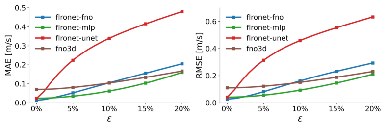
Figure 8: Reconstruction performance under different noise levels: We compare the reconstruction performance of FLRONet-based models and FNO3D under varying levels of noise $\epsilon$. FLRONet-MLP, by leveraging global patterns without relying heavily on spatial dependencies, is less affected by noise. In contrast, FLRONet-UNet propagates noise directly through its skip connections in the branch network with insufficient processing, making it significantly more sensitive to noise. Fourier-based methods like FLRONet-FNO and FNO-3D effectively filter noise through spectral transformations and mode truncations, providing robust performance across noise levels.

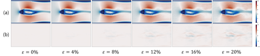
Figure 9: Reconstruction performance of FLRONet-FNO under sensor noise. Row (a) depicts the reconstructed vector field, whereas row (b) displays the associated MAE map. The structural integrity of the reconstructed vector field remains intact at $\epsilon=12\%$.

Fig. 8 indicates that FLRONet-MLP demonstrates strong resilience to noise across all levels of $\epsilon$. Unlike other architectures, FLRONet-MLP does not employ Voronoi embedding, meaning that noise affecting a sensor at a particular position does not propagate to its neighboring regions. Additionally, the MLP branch net models the sensory measurements independently. It relies on the global interactions across the entire input space rather than the localized spatial relationships. This formulation inherently limits the impact of local noise, as perturbations in a small subset of input features can be offset in the dense network. Fig. 8 shows that while FLRONet-MLP is less competitive than FLRONet-FNO under noise-free inputs, it achieves the lowest MAE and RMSE across almost all noise levels. Its error increases only gradually as $\epsilon$ rises from $0\%$ to $20\%$.

On the other hand, FLRONet-UNet is much more affected by noise because its skip connections propagate both noise and useful features directly to the output with insufficient processing. As seen in the figure, FLRONet-UNet shows a sharp increase in both MAE and RMSE even with small $\epsilon$. At $\epsilon=10\%$, its MAE exceeds 0.25 m/s, and at $\epsilon=20\%$, its RMSE surpasses 0.5 m/s, making it the least robust model under noisy conditions.

FLRONet-FNO and FNO-3D models are notably effective at managing noise as a result of their utilization of spectral transformations and mode truncations. These methods transform the input data in the frequency domain and eliminate redundant high-frequency modes that are often noise-dominated. As illustrated in Fig. 8, FLRONet-FNO outperforms FNO-3D when $\epsilon<10\%$. It is crucial to acknowledge that FLRONet-FNO only filters noise in the spatial domain through its two-dimensional Fourier transformation and mode truncations. Conversely, FNO-3D filters noise in both spatial and temporal dimensions. The FNO-3D’s resistance to elevated noise levels is improved by the additional temporal filtering.

Although FLRONet-FNO is not strictly the most robust model for handling noisy data compared to FLRONet-MLP and FNO-3D, it remains a practical method in noisy environments due to its strengths. As shown in later sections, these strengths include highly efficient super-resolution in both space and time. While FLRONet-MLP is completely incapable of doing spatial super-resolution and FNO-3D is also able to achieve super-resolution in both space and time, later analysis shows that FNO-3D is less efficient than FLRONet-FNO. Moreover, FLRONet-FNO achieves superior performance under reasonable noise levels. Fig. 9 indicates that FLRONet-FNO outperforms FNO-3D when $\epsilon\leq 10\%$. Even as the noise level increases to $\epsilon=12\%$, some distortions become visible as seen in Fig. 8; however, the overall flow structures is well-preserved. In practice, sensors are unlikely to generate errors over 10%. In such scenarios, FLRONet-FNO is a better option than FNO-3D due to its versatility, efficiency, and strong performance.

IV.4 Zero-shot super resolution in spatial domain

In contrast to MLP-based or CNN-based architectures, which are inherently resolution-dependent, FLRONet-FNO has a distinctive flexibility that renders it especially useful for applications requiring irregular meshes or diverse resolutions. Standard MLP-based or CNN-based architectures typically require retraining for different spatial scales, hence limiting their practical applicability. In contrast, FLRONet-FNO can reconstruct the complete flow field at arbitrary scales, constrained only by hardware memory.

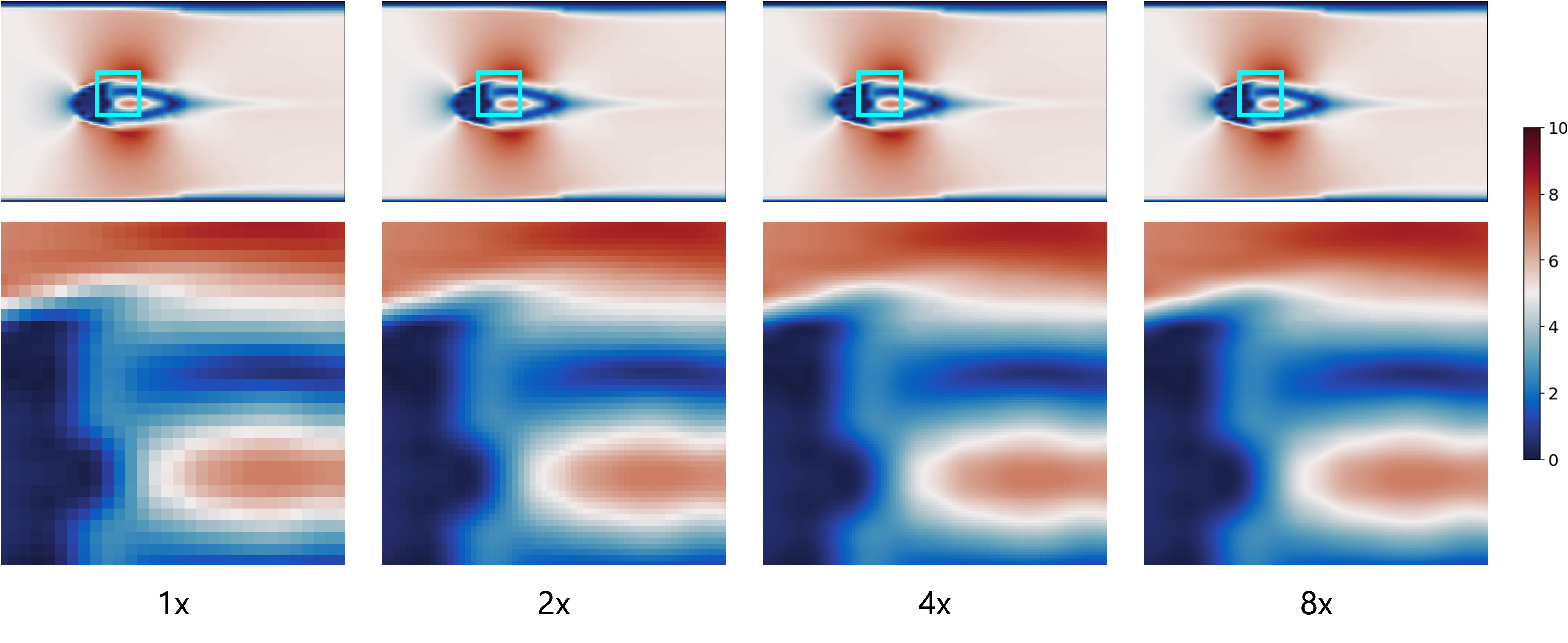
Figure 10: Super-resolution in space: The top row shows the full-field reconstruction, the bottom row provides magnified views of the highlighted regions to illustrate the improvement in spatial detail. Here, we can see the progressive reduction in pixelation and enhancement of spatial details as the resolution increases. Theocratically, FLRONet-FNO is able to reconstruct the complete vector field at arbitrary scales, constrained only by hardware memory.

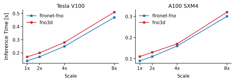
Figure 11: Measured Inference Time for Zero-Shot Super Resolution in Space: The average inference time per time step for FLRONet-FNO and FNO-3D. We test on four different spatial scales $\{1x;2x;4x;8x\}$ using two popular GPUs: Tesla V100 (32GB) and A100 SMX4 (40GB). FLRONet-FNO consistently achieves lower inference times than FNO-3D at all scales.

FLRONet-FNO utilizes Fourier layers to reconstruct the physical field in the functional space. This approach allows the model to be trained on lower-resolution data while still being able to predict at higher resolutions without the need of retraining. The zero-shot super-resolution is feasible because FLRONet-FNO treats both inputs and outputs as continuous functions. During inference at higher spatial resolutions, the models naturally interpolate intermediate values using the predicted continuous function. As a result, knowledge learned from low-resolution data can be directly transferred to high-resolution settings, promoting efficiency and scalability. Fig. 10 demonstrates such capability of FLRONet-FNO. Here, the model was trained on a resolution of $140\times 240$ and make inference on the resolution of $280\times 480$, $560\times 960$, and $1120\times 1920$ which scale up the resolution twice, four, and eight times, respectively. The 8x reconstruction requires approximately 30GB of VRAM, which is well within the capacity of most modern GPUs. Higher-end GPUs e.g. NVIDIA’s A100 with 80GB VRAM or the H100 series can even accommodate 16x reconstructions, providing exceptionally fine-grain details.

The only comparable method that is also capable of performing super-resolution in space is FNO-3D. Both FLRONet-FNO and FNO-3D incur most of their computational cost from the Fourier transformations and their inverses. Consequently, the inference time for both models scales as $O(S\log(S))$, where $S$ represents the spatial resolution of the output. This theoretical analysis is somewhat evident in Fig. 11, in which we measure the average inference time of each model on two popular mid-range GPUs: Tesla V100 (32GB) and A100 SMX4 (40GB). As we expected, the increase in inference time nearly follows a linear-logarithmic pattern. However, FLRONet-FNO slightly achieves lower inference time across all resolutions on both GPUs. The efficiency gap between the two models is more pronounced on the Tesla V100, a lower-FLOPS GPU. These empirical results signify the computational advantage of FLRONet-FNO, particularly on lower-FLOPS hardwares.

IV.5 Zero-shot super resolution in temporal domain

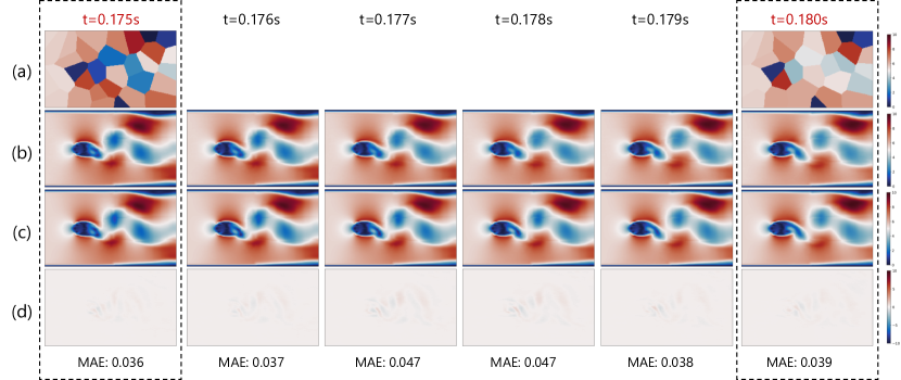
Figure 12: Reconstruction results under the boundary condition $v_{0}=3.5$ m/s: (a) The input Voronoi map at sensory time steps. (b) The reconstructed velocity field predicted by the model. (c) The ground truth velocity field. (d) The Position-wise MAE map between the reconstructed vector field and the ground truth. The aggregated MAE values are provided below each time step to quantify the reconstruction accuracy.

‘

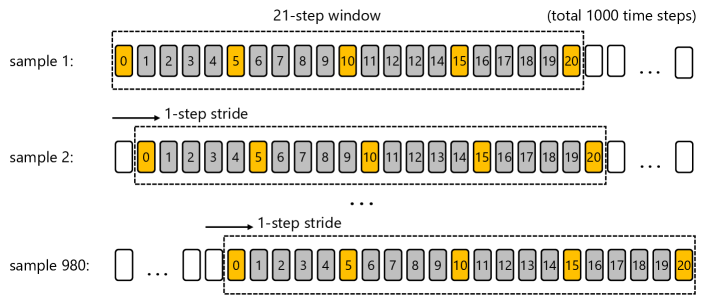
Figure 13: The data generation from CFD dataset: A $21$-step sliding window is applied sequentially across $1,000$ time steps with a stride of $1$, generating $980$ samples for each case of boundary conditions. Each sample consists of $21$ consecutive time steps indexed from $0$ to $20$. The sensory frames are at indices $\{0;5;10;15;20\}$. The models are trained and evaluated on its ability to reconstruct the complete velocity field at any index from $0$ to $20$.

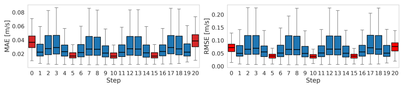
Figure 14: Reconstruction performance at each step in the sliding window: Steps corresponding to sensory inputs (indices $\{0;5;10;15;20\}$) consistently achieve the lowest errors, with minimal variability in both MAE and RMSE values. Predictions tend to be more accurate when made closer to the sensory inputs or towards the center of the sliding window. Predictions at indices $\{2;3;7;8;12;13;17;18\}$ exhibit higher errors as they are temporally furthest from the sensory inputs at $\{0;5;10;15;20\}$. This trend aligns with the expected challenge of predicting further from observed data points. Notably, predictions at indices $\{0;20\}$ also exhibit higher errors despite being sensory input steps, as they are located at the edges of the sliding window and receive only partial temporal context compared to interior steps.

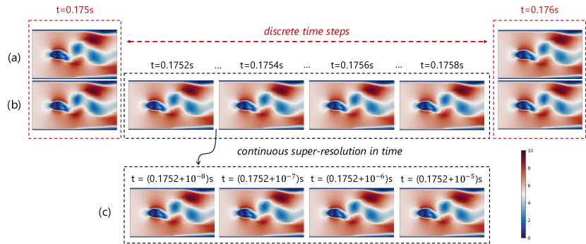
Figure 15: Continuous Super-Resolution in Time: Row (a) shows the true velocity fields provided by the CFD dataset at discrete time steps $t=0.175$s and $t=0.176$s. Row (b) presents the reconstructed velocity fields at intermediate time points $t\in\{0.1750;0.1752;0.1754;0.1756;0.1758;0.1760\}$s, highlighting the model’s ability to continuously generate smooth transitions between consecutive discrete steps. Row (c) further showcases the capability of temporal super-resolution by presenting reconstructions at finer time: $t=(0.1752+10^{-8})$s, $t=(0.1752+10^{-7})$s, $t=(0.1752+10^{-6})$s, and $t=(0.1752+10^{-5})$s.

One of the most notable feature of FLRONet is the ability to perform zero-shot super resolution in the temopral domain, especially in the periods when vortex shredding occurs. In this period, the flow experience highly unstable condition and therefore the capability of acquire finer detail in the temporal domain is crucial. Zero-shot temporal super-resolution refers to the ability of FLRONet to achieve high-resolution temporal predictions from the input sensor data obtained at lower temporal resolution. In other words, it denotes the capability of the model to reconstruct the flow field for any given time within the observational window without knowing the sensor value at such a given time (see Fig. 12).

Fig. 12 illustrates the zero-shot temporal super resolution capability of FLRONet-FNO. The model is trained to utilize sensory data from five evenly-spaced time steps within an interval $\Delta_{t}=0.02$s, and predict the complete physical field at any arbitrary time $t$ within this interval. In this particular example, FLRONet-FNO observes sensory measurements at $t\in\{0.165,0.170,0.175,0.180,0.185\}$ and generates four distinct predictions at intermediate time steps $t^{\prime}\in\{0.176,0.177,0.178,0.179\}$. The true velocity fields at these time steps $t^{\prime}$ are available in the CFD dataset, allowing a direct evaluation. As shown in Fig. 12, FLRONet-FNO achieves highly accurate reconstructions compared to the ground truth. From the MAE plots in row (d), the maximum MAE for the zero-shot temporal super resolution is only $0.047$ m/s, occurring at the frames furthest from the sensory inputs. At frames that are close to or exactly at the sensory inputs, MAE values only range from $0.036$ m/s to $0.039$ m/s. This specific interval was intentionally chosen for such qualitative evaluation because it represents the most turbulent period in the simulation. This period exhibits the transition from laminar flow to vortex shedding. The ability of FLRONet-FNO to maintain accuracy even during such a complex dynamic transition demonstrated its effectiveness in handling turbulence in typical fluid flow problems.

In order to provide a complete evaluation, we conducted the same prediction process at different windows. In particular, given the temporal resolution of the CFD dataset is 0.001s, we slide a window of length $\Delta_{t}=0.2$s along the temporal domain of length $T=1.0$s, generating 980 samples for each case of test boundary conditions. As depitcted in Fig. 13, each sample is captured by a 21-step window with its time steps being indexed from $0$ to $20$. For each sample, we make 21 independent predictions for every available time steps from the first sensory input (indexed at $0$) to the fifth sensory input (indexed at $20$). Since we have 5 cases of boundary conditions in our test set, we are able to make $21\times 980\times 5=102,900$ predictions. We collect the MAE and RMSE values of all predictions to evaluate the ability of FLRONet-FNO in reconstructing arbitrary time that has different temporal distances to sensory inputs. The results are reported in Fig. 14.

Fig. 14 provides a detailed breakdown of the performance metrics presented in Fig. 5. The overall performance of FLRONet-FNO is superior to all baselines. Nevertheless, there is a little variation in prediction errors depending on the temporal proximity of the predicted time step to the sensory inputs. Predictions near the sensory input steps (indices $\{0,5,10,15,20\}$) consistently show lower errors. This demonstrates the model’s ability to effectively utilize direct observations. In contrast, predictions at time farthest away from the sensory inputs tend to have relatively higher errors. This behavior reflects the difficulty of interpolating data at greater temporal distances. Moreover, edge steps at indices $\{0,20\}$ also exhibit higher errors, despite being sensory inputs, this is likely due to the reduced temporal context available at the boundaries of the sliding window. While interior steps benefit from contextual information on both sides, edge steps only have access to half the context. They rely solely on either the information on the left or the right side relative to their current temporal position.

Up to this point, we have shown the ability of FLRONet-FNO to perform temporal super-resolution at the default temporal resolution of the CFD dataset. While this setup enables us to directly evaluate the reconstructed results against the ground truth, it does not demonstrate model’s full potential to scale indefinitely along the temporal dimension. In the results showed in Fig. 14, each step corresponds to $0.001$s, we now explore its capability to predict velocity fields at arbitrary continuous time points $t$. Fig. 15 shows reconstructed velocity fields at some intermediate timestamps between $t=0.175$s and $t=0.176$s. This significantly extends the super-resolution presented in Fig. 12. Although no ground truth exists at such fine temporal resolutions, the reconstructed frames at $t\in\{0.1752;0.1754;0.1756;0.1758\}$ visually describe the smooth transition from the true field at $t=0.175$s to the true field at $t=0.176$s. In fact, FLRONet-FNO can predict the velocity field at any real value of $t\in\mathcal{W}$, where $\mathcal{W}$ is the temporal window of the sensory inputs. To illustrate this, row (c) in Fig. 15 pushes the resolution further by presenting the reconstructed velocity fields at $t=0.1752+10^{-8}$, $t=0.1752+10^{-7}$, $t=0.1752+10^{-6}$, and $t=0.1752+10^{-5}$. We can achieve even higher resolution if required. In theory, continuous super-resolution in time allows predictions at any real value of $t$. In practical settings, the highest possible resolution is limited by the floating-point precision of the data type, defining the smallest time step that can be resolved during calculations.

IV.6 Discussion and implications

The validation study above has justified the reconstruction capability of FLRONet for both reconstruction accuracy and the visual quality of the reconstructed flow field. Here, we emphasize the zero-shot super-resolution capability in both space and time of FLRONet, which is rooted in its operator learning framework.

In industrial applications, capturing high-frequency or high-resolution sensor data is often impractical due to hardware limitations. FLRONet addresses this challenge by offering affordable reconstructions of fine-scale dynamics from sparse sensor data. For example, in this study, the fluid flow geometry around a cylinder has a resolution of $140\times 240$ ($33,600$ possible locations), yet only $32$ sensor locations (approximately 0.095% density) were used for training. Once trained, FLRONet is able to perform full-state reconstruction under varying boundary conditions within milliseconds on a single GPU, eliminating the need of a dedicated computing server that are typically required for traditional numerical methods.

One aspect worth mentioning is that FLRONet is very efficient in performing inference in the continuous temporal domain. This property makes it a much better alternative compared to the three-dimensional FNO (FNO-3D). While FNO-3D is mathematically capable of inferring in continuous time, in practice, its use of the discrete FFT method to approximate the Fourier and inverse Fourier transforms along the temporal dimension constrains it to a finite resolution. FLRONet avoids this limitation by not introducing an extra dimension in the FFT computations. Instead, it relies on a trunk network to model the temporal domain.

Time Complexity Analysis: The computational complexities of FNO-3D and FLRONet primarily arise from their operations in the frequency domain, including complex-valued linear transformations, along with the FFT and its inverse. Let $T$ and $S$ represent the temporal and spatial resolutions, respectively. For FNO-3D, although its linear transformations exhibit a constant time complexity of $O(1)$, all the computational bottleneck comes from the FFT and its inverse. These operations incur the complexity of $O(TS\log(TS))$, this is also the overall complexity of FNO-3D. On the other hand, FLRONet scales linearly with $T$ for its linear transformations, resulting in a complexity of $O(T)$. The FFT and its inverse operations contribute an extra complexity of $O(TS\log(S))$. Dot-product operations in the trunk network and the following fusing operations introduce a computational cost of $O(TS)$. When combined, the total computational complexity of FLRONet becomes $O(TS\log(S)+T+TS)$. This makes FLRONet more efficient than FNO-3D, particularly when $T$ is large.

V Conclusion

This study proved that FLRONet is a more efficient and accurate alternative to FNO-3D for fluid flow reconstruction from a limited number of sensors. We evaluated FLRONet in comparison to FNO-3D under diverse suboptimal settings, including absent sensor readings and inaccurate sensor values. Furthermore, we assessed the time complexity of FLRONet in zero-shot super-resolution across spatial and temporal domains. As shown in Section IV, FLRONet far outperforms FNO-3D in almost all of these scenarios. The complexity analysis in Section IV.6 further indicates that while both FLRONet and FNO-3D exhibit a computational complexity of $O(S\log(S))$ for spatial super-resolution, FLRONet demonstrates greater efficiency than FNO-3D in temporal super-resolution. Given a fixed spatial resolution $S$, FLRONet scales as $O(T)$, whereas FNO-3D scales as $O(T\log(T))$. Furthermore, FLRONet is able to perform super-resolution at arbitrary continuous time points, with the highest achievable temporal resolution constrained only by the floating-point precision of the data type. This capability makes FLRONet particularly well-suited for tasks requiring fast, up-scaled interpolation at any time instances that are covered in a sensory window.

FLRONet architecture is still a subject of further investigation. Particularly, future research might focus on the capacity of FLRONet for temporal extrapolation, which involves evaluating the effectiveness of FLRONet in predicting full flow fields that are beyond the sensory window. This entails assessing its ability to forecast complete flow fields beyond the covered temporal window. If this capability is confirmed, FLRONet may be used in a broader range of applications, such as fluid dynamics modeling and forecasting.

Data Availability

The data and source code that support the findings of this study are available at https://github.com/hiepdang-ml/FLRONet

References

References

- Erichson et al. (2020) N. B. Erichson, L. Mathelin, Z. Yao, S. L. Brunton, M. W. Mahoney, and J. N. Kutz, “Shallow neural networks for fluid flow reconstruction with limited sensors,” Proceedings of the Royal Society A: Mathematical, Physical and Engineering Sciences 476, 20200097 (2020).
- Loiseau, Noack, and Brunton (2018) J.-C. Loiseau, B. R. Noack, and S. L. Brunton, “Sparse reduced-order modelling: sensor-based dynamics to full-state estimation,” Journal of Fluid Mechanics 844, 459–490 (2018).
- Mons et al. (2016) V. Mons, J.-C. Chassaing, T. Gomez, and P. Sagaut, “Reconstruction of unsteady viscous flows using data assimilation schemes,” Journal of Computational Physics 316, 255–280 (2016).
- Wu, Xiao, and Luo (2023) J. Wu, D. Xiao, and M. Luo, “Deep-learning assisted reduced order model for high-dimensional flow prediction from sparse data,” Physics of Fluids 35 (2023), 10.1063/5.0166114.
- Li et al. (2024) R. Li, B. Song, Y. Chen, X. Jin, D. Zhou, Z. Han, W.-L. Chen, and Y. Cao, “Deep learning reconstruction of high-reynolds-number turbulent flow field around a cylinder based on limited sensors,” Ocean Engineering 304, 117857 (2024).
- Cheng et al. (2024) S. Cheng, C. Liu, Y. Guo, and R. Arcucci, “Efficient deep data assimilation with sparse observations and time-varying sensors,” Journal of Computational Physics 496, 112581 (2024).
- Kovachki et al. (2023) N. Kovachki, Z. Li, B. Liu, K. Azizzadenesheli, K. Bhattacharya, A. Stuart, and A. Anandkumar, “Neural operator: Learning maps between function spaces with applications to pdes,” Journal of Machine Learning Research 24, 1–97 (2023).
- Zhao et al. (2024) X. Zhao, X. Chen, Z. Gong, W. Zhou, W. Yao, and Y. Zhang, “Recfno: A resolution-invariant flow and heat field reconstruction method from sparse observations via fourier neural operator,” International Journal of Thermal Sciences 195, 108619 (2024).
- Li et al. (2020) Z. Li, N. B. Kovachki, K. Azizzadenesheli, B. Liu, K. Bhattacharya, A. M. Stuart, and A. Anandkumar, “Fourier neural operator for parametric partial differential equations,” CoRR abs/2010.08895 (2020), 2010.08895 .
- Nguyen et al. (2024) P. C. H. Nguyen, X. Cheng, S. Azarfar, P. K. Seshadri, Y. T. Nguyen, M. Kim, S. Choi, H. S. Udaykumar, and S. Baek, “Parcv2: Physics-aware recurrent convolutional neural networks for spatiotemporal dynamics modeling,” ArXiv abs/2402.12503 (2024).
- Lu et al. (2021) L. Lu, P. Jin, G. Pang, Z. Zhang, and G. E. Karniadakis, “Learning nonlinear operators via DeepONet based on the universal approximation theorem of operators,” Nature Machine Intelligence 3, 218–229 (2021).
- Ronneberger, Fischer, and Brox (2015) O. Ronneberger, P. Fischer, and T. Brox, “U-net: Convolutional networks for biomedical image segmentation,” Medical Image Computing and Computer-Assisted Intervention – MICCAI 2015 , 234–241 (2015).
- Dubois et al. (2022) P. Dubois, T. Gomez, L. Planckaert, and L. Perret, “Machine learning for fluid flow reconstruction from limited measurements,” Journal of Computational Physics 448, 110733 (2022).
- Yining, Yingfa, and Zhen (2023) L. Yining, C. Yingfa, and Z. Zhen, “Cfdbench: A large-scale benchmark for machine learning methods in fluid dynamics,” (2023).