Ptychoformer: A Physics-Guided Deep Learning Framework for Ptychographic Imaging

Abstract

Ptychographic imaging confront limitations in applying deep learning (DL) for retrieval from diffraction patterns. Conventional neural architectures are optimized for natural images, overlooking the unique physical characteristics of diffraction data, including radial intensity decay and coherent information distributed in concentric rings. In this paper, we present Ptychoformer, a physics-guided DL framework for ptychographic imaging that aligns attention mechanisms and feature extraction with these diffraction physics properties through introducing a dual-branch architecture which accounts for both local and non-local dependencies from the patterns. It consists of a Polar Coordinate Attention (PCA) mechanism that is inspired by the Ewald construction in X-ray crystallography to enhance high-frequency component fidelity. Experimental results demonstrate Ptychoformer’s superior performance across both simulated and real data in preserving fine details and suppressing artifacts. On simulated data, Ptychoformer achieves up to 5.4% higher PSNR and 4.2% higher SSIM for amplitude retrieval compared to existing methods. For real experimental data, it demonstrates up to 12.5% higher PSNR and 31.3% higher SSIM for amplitude retrieval. Notably, Ptychoformer maintains robust performance under limited training data and low overlap ratios, outperforming existing models.

I Introduction

Coherent diffraction imaging (CDI) has enabled high-resolution, lens-less imaging across various scientific disciplines by exploiting the principles of wave propagation and interference. In CDI, detectors capture only the far-field intensity distribution of scattered coherent radiation, resulting in the loss of crucial phase information due to the well-known phase problem in crystallography. The objective of phase retrieval algorithms is to reconstruct the complete complex-valued exit wave function from these incomplete Fraunhofer diffraction patterns. Ptychography [1] , an advanced CDI technique that operates in both real and reciprocal space, addresses this inverse problem by utilizing multiple overlapping diffraction measurements in reciprocal space, effectively extending the Fourier domain sampling and enabling robust phase retrieval through iterative algorithms. This approach offers extended field-of-view imaging with exceptional spatial resolution in real space. Recent breakthroughs have pushed the boundaries of resolution, achieving $0.39\text{\,}\mathrm{\SIUnitSymbolAngstrom}$ in transmission electron microscopy [2] and even $14\text{\,}\mathrm{pm}$ through local-orbital ptychography [3], opening new possibilities in materials characterization [4], biological imaging [5], and semiconductor research[6].

Figure 1: Diffraction pattern characteristics and diffraction physics. (a): Diffraction patterns exhibit a radial distribution of information, with varying requirements for capturing low and high-frequency information. (b): 2D diffraction patterns can be viewed as projections of the intersection between the Ewald sphere and the crystal onto the detector plane. Sphere’s radius is $1/\lambda$, the wavelength of the incident and diffracted beams. Importantly, the spatial adjacency preference observed in natural images’ feature space also holds in the polar coordinate perspective of diffraction patterns.

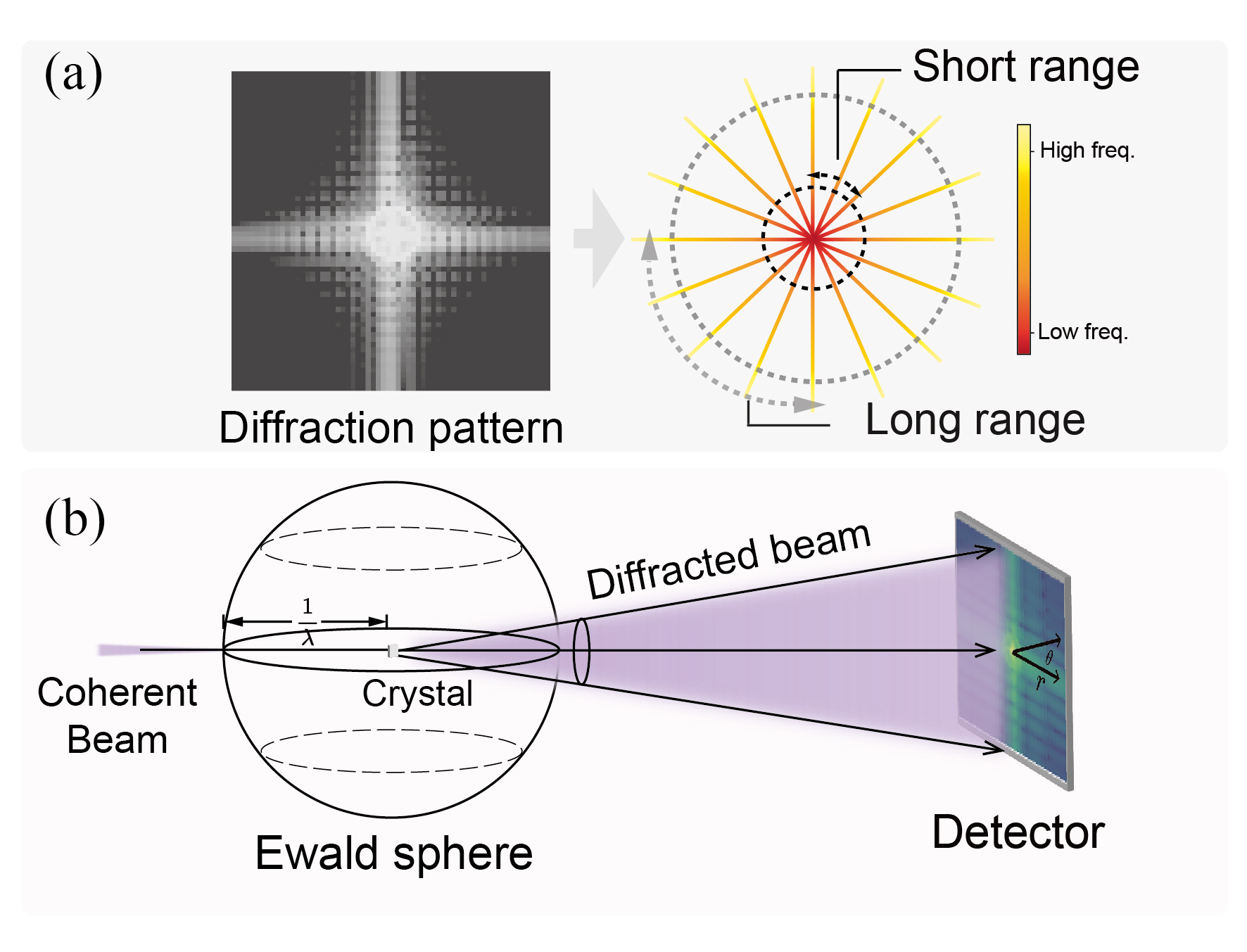
However, the widespread application of ptychography faces significant challenges, particularly in computational efficiency. As imaging capabilities advance, data volume grows exponentially, overwhelming conventional algorithms. For instance, processing one second of data from a modern synchrotron source (10-megapixel detector, 32-bit depth, 2 kHz, 640 Gb/s) can take up to an hour [7]. Additionally, achieving high-quality retrievals requires 60-70% probe position overlap [8], further increasing computational complexity. These factors severely constrain ptychography’s viability in real-time and high-throughput applications.

To address these limitations, researchers have redefined ptychography as a data-driven supervised learning task, leveraging deep learning (DL) techniques. Notable examples including PtychoNN [9], Deep-phase-imaging (DPI) [10], and PtyNet [11] have demonstrated improved retrieval efficiency. Unlike conventional approaches that require repeated iterations across the spatial and frequency domains, these methods utilize experimentally acquired diffraction patterns and complex amplitude images reconstructed by traditional algorithms as training data. Through convolutional neural network (CNN) based architectures, they establish a direct mapping from diffraction patterns to complex amplitude retrieval, significantly enhancing computational efficiency. Despite their success, CNN-based methods face challenges in processing multi-frequency information, capturing long-range correlations, and distinguishing high-frequency signals from noise in diffraction patterns, as illustrated in Fig. 1(a). These limitations are due to the sliding window operation of convolution kernels in spatial coordinates and the information flattening in multi-layer convolution during transmission [12, 13, 14]. Transformer models, while powerful in various computer vision tasks, have limited application in ptychography due to the mismatch between their design principles and the radial nature of diffraction patterns. For instance, Vision Transformers (ViT), are primarily optimized for natural images in real space (e.g., patch extraction operations and local feature preference priors of the Softmax function). However, these priors do not directly map to the radial nature of diffraction data in reciprocal space shown in Fig. 1(a).

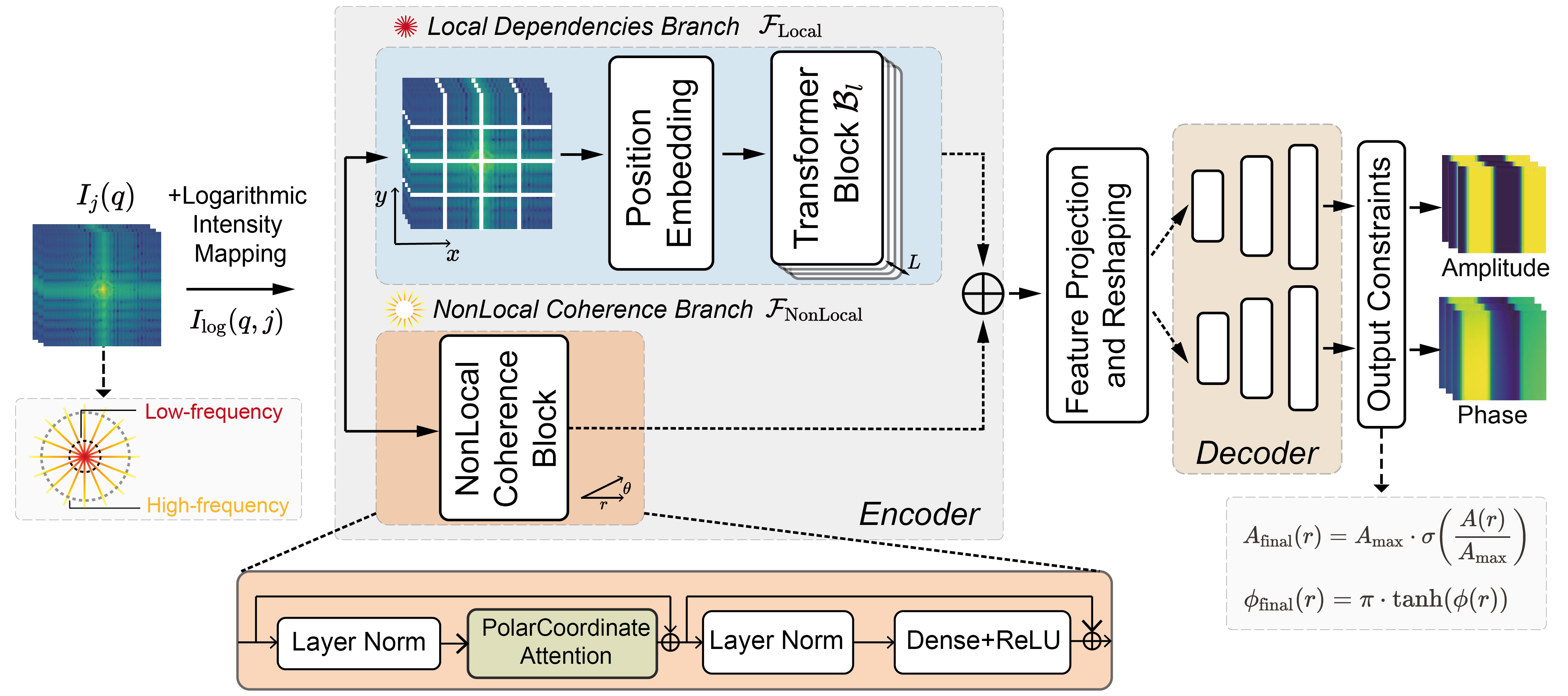
Addressing the inherent limitations of existing methods requires a fundamental reconsideration of deep learning architectures for ptychographic retrieval, with a focus on optimizing neural networks for representing diffraction patterns in reciprocal space. This insight guided the development of Ptychoformer, a novel framework that bridges frequency-domain diffraction patterns and real-space images using physics-informed deep learning techniques. Drawing inspiration from the Ewald construction in X-ray crystallography, as depicted in Fig. 1(b), treating 2D diffraction patterns as projections of the intersections between the Ewald sphere and the reciprocal lattice onto the detector plane, as shown in the left of Fig. 1. This insight revealed that diffraction patterns are inherently defined in spherical rather than planar geometry. Consequently, we developed Polar Coordinate Attention (PCA), an attention mechanism leveraging polar coordinates that naturally aligns with diffraction physics. This polar coordinate-based attention mechanism reframes real-space structural priors in the diffraction context, mapping scattering vector magnitude to $r$ and angular information to $\theta$, thus capturing both radial intensity attenuation and angular coherence. Recognizing the multi-scale and multi-frequency nature of diffraction patterns, as shown in the right side of Fig. 1, Ptychoformer employs a dual-branch architecture combining a Local Dependencies Branch constructed from standard ViT blocks with a NonLocal Coherence block containing our designed PCA. This design balances the capture of long-range and local dependencies in diffraction patterns. Ptychoformer’s architecture intrinsically aligns with ptychography physics, creating a more natural correspondence between model operations and underlying physical processes.

This structural redesign based on physical insights enables our model to more effectively extract and utilize global coherent information and long-range dependencies in diffraction data, thus offering a physics-informed approach to ptychographic retrieval. Our comprehensive experiments on both simulated and real datasets demonstrate Ptychoformer’s significant advantages over existing state-of-the-art methods, particularly in high-frequency artifact suppression and data efficiency. Under challenging conditions including low overlap ratios, and limited training data, our model maintains superior retrieval quality, achieving up to 36.1% reduction in Mean Squared Error (MSE) and 12.03% increase in Structural Similarity Index Measure (SSIM) compared to the best-performing existing end-to-end methods. These improvements could significantly enhance the applicability of ptychography in time-sensitive or radiation-sensitive imaging scenarios across various scientific disciplines.

The primary contributions of this work are summarized as follows:

• We present Ptychoformer, an end-to-end deep learning framework addressing limitations of existing DL-based ptychography methods. Unlike conventional neural architectures optimized for spatial-domain natural images, our approach incorporates designs aligned with diffraction physics.

• We propose the PCA mechanism, a physics-inspired approach that decomposes attention into radial and angular components, enabling efficient extraction of coherent information across frequency bands in diffraction patterns.

• Extensive experiments on both simulated and real datasets show that the proposed method achieves high-fidelity and superior artifact reduction, while maintaining efficiency under challenging conditions including noisy environments and limited data acquisition scenarios.

II Related Works

II-A Deep Learning-Based Ptychographic Imaging

Deep learning in ptychographic imaging has recently enhanced computational efficiency and retrieval quality, categorized into three strategies:

II-A1 Pre-processing

Integrating deep learning with iterative algorithms improves initial estimates. The physics-informed automatic differentiation ptychography (ADP) framework uses pre-trained autoencoders to map high-dimensional image data to a low-dimensional latent space [15], while the double deep image prior (DDIP) method reduces the optimization parameter space [16], both enhancing convergence rates and noise robustness.

II-A2 Post-processing

Neural networks refine reconstructions from traditional algorithms, including enhancing a single iteration of the Gerchberg-Saxton-Fienup (GSF) algorithm to improve spatial resolution and reduce artifacts [5], showing promise in live cell imaging.

II-A3 End-to-End

End-to-end methods directly map diffraction patterns to complex object functions, bypassing iterative processes. Examples include PtychoNN with a modified U-Net and two-branch decoder for amplitude and phase [9], PtyNet with group convolution and Leaky ReLU for efficiency [11], and DPI using a traditional U-Net with skip connections [10].

Despite improved retrieval speed, these methods face challenges to preserve high-frequency information and the global coherence of diffraction patterns, as CNNs and standard Vision Transformers (ViTs) are tailored for real-space images with local correlations. Recent studies using ViTs for ptychographic retrieval leverage self-attention for long-range dependencies [17], but applying ViT architectures to frequency-domain data is limited by radial intensity decay and concentric information distribution. Addressing these frequency-domain challenges, including processing global coherence and preserving high frequencies, remains crucial for advancing retrieval quality and efficiency, especially with limited data or low overlap ratios.

II-B ViT-based Methods

Figure 2: The proposed Ptychoformer architecture for ptychographic imaging. It features dual branches: a Local Dependencies Branch with standard ViT blocks, and a NonLocal Coherence Branch with PolarCoordinate Attention mechanism. The model processes logarithmically mapped diffraction patterns, combining features from both branches before decoding into amplitude and phase images with physical constraints applied.

Diffraction patterns, governed by wave optics, approximate the Fourier transform of an object’s transmission function in far-field conditions [18], resulting in reciprocal space features like sparse representations and concentric rings [19]. Accurate image retrieval and phase retrieval require effectively capturing both sparsity and long-range dependencies within these patterns. Traditional CNNs, though effective for natural images [20, 21], are limited with the global nature of diffraction phenomena due to their local receptive fields. Vision Transformers (ViTs), introduced by Dosovitskiy et al. [22], offer a promising alternative with self-attention mechanisms that capture global features and long-range dependencies [23], outperforming CNNs in various computer vision tasks [24, 25] and extending to fields like medical image segmentation [24, 26], climate modeling [27], and molecular structure prediction [28]. However, applying ViTs to phase retrieval in CDI is challenging due to the lack of CNN-like inductive biases such as translational invariance and local connectivity, coupled with often insufficient data in practical phase imaging. For example, PtychoDV [17] uses ViTs for feature extraction from diffraction patterns but shows inferior retrieval performance compared to CNN-based U-Net architectures without iterative post-processing. This gap highlights the potential for developing hybrid methods that leverage transformers’ global feature extraction while addressing data limitations in ptychography.

III Methodology

III-A Problem Formulation

In ptychography, we aim to reconstruct a complex-valued object function $O(\mathbf{r})$, where $\mathbf{r}$ is the position vector in real space. This retrieval is based on a set of diffraction patterns measured at spatial frequencies $\mathbf{q}$ in reciprocal space. The process involves a probe function $P(\mathbf{r})$, which interacts with the object at various scanning positions $\{\mathbf{r}_{j}\}_{j=1}^{J}$. The ptychography problem can be formulated as:

$$\mathcal{F}\{\psi_{j}(\mathbf{r})\}=\sqrt{I_{j}(\mathbf{q})}\cdot\exp(i\phi_{j}(\mathbf{q}))$$ (1)

where $\psi_{j}(\mathbf{r})=P(\mathbf{r}-\mathbf{r}_{j})\cdot O(\mathbf{r})$ is the exit wave function, $\mathcal{F}$ denotes the Fourier transform, $I_{j}(\mathbf{q})$ is the measured diffraction intensity, and $\phi_{j}(\mathbf{q})$ is the phase of the diffraction pattern.

To account for real-world factors, we model the diffraction intensity as:

$$\begin{split}I_{j}(\mathbf{q})=&\mathcal{P}_{\eta}\left(\eta\left|\mathcal{F}\left\{\mu P(\mathbf{r}-\mathbf{r}_{j}-\delta\mathbf{r}_{j})O(\mathbf{r})\right.\right.\right.\\ &\left.\left.\left.+(1-\mu)P(\mathbf{r}-\mathbf{r}_{j}-\delta\mathbf{r}_{j})\mathbb{E}_{\mathbf{r}}[O(\mathbf{r})]\right\}\right|^{2}\right)\\ &+\mathcal{N}(0,\sigma^{2})\end{split}$$ (2)

where $\mu$ is the coherence parameter, $\eta$ is the detector efficiency, $\mathcal{P}_{\eta}$ models Poisson shot noise, $\mathcal{N}(0,\sigma^{2})$ represents Gaussian noise, and $\delta\mathbf{r}_{j}$ accounts for positional jitter. The objective function for ptychographic retrieval is defined as:

$$\begin{split}\mathcal{J}(O,P)=&\frac{1}{J}\sum_{j=1}^{J}\left\|I_{j}-|\mathcal{F}\{P(\mathbf{r}-\mathbf{r}_{j})\cdot O(\mathbf{r})\}|^{2}\right\|_{2}^{2}\\ &+\lambda_{1}\Omega_{1}(O)+\lambda_{2}\Omega_{2}(P)\end{split}$$ (3)

where $\left\|\mathbf{x}\right\|_{2}^{2}=\sum_{i}x_{i}^{2}$ is the squared Euclidean norm, $\Omega_{1}(O)=\left\|\nabla O\right\|_{1}$ enforces sparsity in the object gradient, $\Omega_{2}(P)=\left\|P-P_{0}\right\|_{2}^{2}$ constrains the probe function to maintain proximity to to an initial estimate $P_{0}$, and $\lambda_{1}$ and $\lambda_{2}$ are regularization weights.

III-B Ptychoformer Architecture

Figure 3: Architectural overview of the PCA mechanism. The diagram illustrates the flow of input features through polar coordinate transformation, query-key-value attention computations, and subsequent operations including polar coordinate weighting and Hadamard product. The process culminates in multi-head attention, followed by concatenation and linear projection to produce the final output.

The Ptychoformer architecture uses a bifurcated structure to map diffraction patterns to a reconstructed complex-valued object function. The input undergoes a logarithmic transformation $I_{\text{log}}(\mathbf{q},j)=\log(1+I_{j}(\mathbf{q}))$ as a preprocessing step to address the large disparity between high and low frequency values in the diffraction patterns.

III-B1 Local Dependencies Branch

The Local Dependencies Branch employs a standard ViT to analyze diffraction patterns, aiming to capture local features and relationships within the pattern. The branch’s structure consists of several key components. Initially, a patch extraction mechanism segments the diffraction pattern into smaller sections. These segments then undergo reshaping to facilitate subsequent processing. Following this, an encoding step is applied to each patch, designed to emphasize relevant features. The encoded patches are then processed through a series of ViT blocks. Each ViT block $\mathcal{B}_{l}$ in $\mathcal{B}_{L}$ is defined as:

$$\begin{split}\mathcal{B}_{l}(\mathbf{X})&=\mathbf{X}+\mathcal{FFN}(\mathcal{LN}(\mathbf{X}+\mathcal{MSA}(\mathcal{LN}(\mathbf{X}))))\\ \mathcal{MSA}(\mathbf{X})&=\text{Concat}(\text{head}_{1},\ldots,\text{head}_{h})\mathcal{W}^{O}\\ \text{head}_{i}&=\text{Attention}(\mathbf{X}\mathcal{W}^{Q}_{i},\mathbf{X}\mathcal{W}^{K}_{i},\mathbf{X}\mathcal{W}^{V}_{i})\end{split}$$ (4)

where $\mathcal{LN}$ denotes layer normalization, $\mathcal{MSA}$ is multi-head self-attention with $h$ heads, $\mathcal{FFN}$ is a position-wise feed-forward network, and $\mathcal{W}^{Q}_{i},\mathcal{W}^{K}_{i},\mathcal{W}^{V}_{i},\mathcal{W}^{O}$ are learnable weight matrices. Despite apparent disruption, patch extraction facilitates low-frequency information capture, especially from central patches containing crucial low-frequency components.

III-B2 NonLocal Coherence Branch

The NonLocal Coherence Branch operates directly on the full-resolution input, intentionally omitting patch extraction to preserve the global structure of the diffraction pattern. It replaces the multi-head self-attention in standard ViT blocks with PCA, and the radial information introduced by PCA eliminates the need for position embeddings.

While traditional self-attention mechanisms are effective for capturing long-range dependencies, they are not optimized for ptychographic data. Designed for natural images, they incorporate spatial positional encodings $\text{PE}(p)$ that can bias attention towards local regions: $A_{pq}=\text{softmax}(\frac{(x_{p}+\text{PE}(p))^{T}(x_{q}+\text{PE}(q))}{\sqrt{d_{k}}})$. This provides structural priors suited for conventional visual tasks but may not be optimal for frequency-domain diffraction patterns. To address this limitation, we introduce the PCA mechanism. PCA transforms spatial coordinates into polar coordinates, shifting the structural priors from Cartesian spatial locality to the concentric information distribution inherent in frequency-domain diffraction patterns. This transformation enables PCA to better capture the radial and angular dependencies characteristic of ptychographic data. The PCA layer $\mathcal{PCA}:\mathbb{R}^{B\times H\times W\times C}\to\mathbb{R}^{B\times H\times W\times C^{\prime}}$ is defined as:

$$\mathcal{PCA}(\mathbf{X})=\text{Reshape}(\mathcal{F}(\text{Flatten}(\mathbf{X})))$$ (5)

$$\mathcal{F}(\mathbf{X})=\text{Concat}(\text{Head}_{1},\text{Head}_{2},\dots,\text{Head}_{h})\mathcal{W}_{O}$$ (6)

$$\text{Head}_{i}=\text{softmax}(\mathcal{A}r^{i}(\mathbf{X})+\mathcal{A}\theta^{i}(\mathbf{X}))\mathcal{V}^{i}(\mathbf{X})$$ (7)

$$\mathcal{A}r^{i}(\mathbf{X})=\frac{\mathcal{Q}^{i}(\mathbf{X})\mathcal{K}^{i}(\mathbf{X})^{T}}{\sqrt{d_{k}}}\odot\mathbf{R}$$ (8)

$$\mathcal{A}\theta^{i}(\mathbf{X})=\frac{\mathcal{Q}^{i}(\mathbf{X})\mathcal{K}^{i}(\mathbf{X})^{T}}{\sqrt{d_{k}}}\odot\mathbf{\Theta}$$ (9)

where $\mathcal{Q}^{i},\mathcal{K}^{i}\in\mathbb{R}^{N\times d_{k}}$, $\mathcal{V}^{i}\in\mathbb{R}^{N\times d_{v}}$ are the linear projections for queries, keys, and values for the $i$-th head, $d_{k}$ is the dimension of the keys, $\mathbf{R},\mathbf{\Theta}\in\mathbb{R}^{N\times N}$ are the normalized radial and angular coordinate matrices, respectively, $\odot$ denotes the Hadamard product (element-wise multiplication), and $\mathcal{W}_{O}\in\mathbb{R}^{hd_{v}\times C^{\prime}}$ is the output projection matrix. Here, $N=H\times W$ is the number of spatial positions. The coordinate matrices are computed as:

$$R_{ij}=\frac{\sqrt{(i-W/2)^{2}+(j-H/2)^{2}}}{\sqrt{(W/2)^{2}+(H/2)^{2}}}$$ (10)

$$\Theta_{ij}=\frac{\arctan 2(j-H/2,i-W/2)}{\pi}$$ (11)

where $i\in[1,W]$ and $j\in[1,H]$ are the horizontal and vertical indices of the spatial positions, respectively. This mechanism decomposes attention into radial and angular components, mirroring the symmetry of diffraction patterns. Operating without patch extraction, this branch preserves global structure. Its polar coordinate attention is designed to extract global coherence information, particularly high-frequency components requiring long-range dependency modeling.

III-B3 Feature Fusion and Decoding

Let $\mathcal{F}_{\text{Local}}:L^{2}(\mathbb{R}^{2}\times\{1,\ldots,J\})\to\mathcal{H}_{\text{Local}}$ and $\mathcal{F}_{\text{NonLocal}}:L^{2}(\mathbb{R}^{2}\times\{1,\ldots,J\})\to\mathcal{H}_{\text{NonLocal}}$ denote the feature extraction operators from the Local Dependencies Branch and the NonLocal Coherence Branch, respectively. The decoder is defined as a composition of three upsampling operators $\mathcal{D}=\mathcal{D}_{3}\circ\mathcal{D}_{2}\circ\mathcal{D}_{1}$, each progressively increasing the spatial resolution using transposed convolutions. Here, $\circ$ denotes function composition, such that $(f\circ g)(x)=f(g(x))$ for any compatible functions $f$ and $g$. The feature fusion process, combining features from both branches, is formulated as:

$$\mathcal{F}_{\text{fused}}=\mathcal{C}(\mathcal{F}_{\text{Local}},\mathcal{F}_{\text{NonLocal}})$$ (12)

where $\mathcal{C}$ concatenates $\mathcal{F}_{\text{Local}}$ and $\mathcal{F}_{\text{NonLocal}}$, followed by a convolution to integrate the features. The fused features $\mathcal{F}_{\text{fused}}$ are then processed through the three-layer decoder $\mathcal{D}$, implemented using transposed convolutions with batch normalization and ReLU activations, split into parallel branches $\mathcal{D}_{\text{amplitude}}$ and $\mathcal{D}_{\text{phase}}$, to reconstruct the preliminary amplitude $\mathbf{A}(\mathbf{r})$ and phase $\boldsymbol{\phi}(\mathbf{r})$ images.

III-B4 Output Constraints

To ensure the physical validity of the reconstructed complex-valued object function, we apply constraints to the final outputs. The amplitude $\mathbf{A}_{\text{final}}:\mathbb{R}^{2}\to\mathbb{R}^{+}$ and phase $\boldsymbol{\phi}_{\text{final}}:\mathbb{R}^{2}\to[-\pi,\pi]$ are constrained as:

$$\mathbf{A}_{\text{final}}(\mathbf{r})=A_{\text{max}}\cdot\sigma\left(\frac{\mathbf{A}(\mathbf{r})}{A_{\text{max}}}\right),\quad\boldsymbol{\phi}_{\text{final}}(\mathbf{r})=\pi\cdot\tanh\left(\boldsymbol{\phi}(\mathbf{r})\right)$$ (13)

where $A_{\text{max}}$ is the maximum allowable amplitude, $\sigma$ is the sigmoid function, and $\tanh$ is the hyperbolic tangent function. The final complex-valued object function is reconstructed as

$$O_{\text{reconstructed}}(\mathbf{r})=\mathbf{A}_{\text{final}}(\mathbf{r})\cdot\exp\left(i\boldsymbol{\phi}_{\text{final}}(\mathbf{r})\right).$$

III-B5 Training Objective

The loss function $\mathcal{L}:\Theta\to\mathbb{R}^{+}$ is defined as:

$$\mathcal{L}(\theta)=\frac{1}{N}\sum_{n=1}^{N}\left[\left\|A_{\text{true}}^{(n)}-A_{\text{pred}}^{(n)}\right\|_{2}^{2}+\left\|\phi_{\text{true}}^{(n)}-\phi_{\text{pred}}^{(n)}\right\|_{2}^{2}\right]$$ (14)

where $N$ is the number of training samples, $A_{\text{true}}^{(n)}$ and $\phi_{\text{true}}^{(n)}$ are the true amplitude and phase for the $n$-th sample, respectively, and $A_{\text{pred}}^{(n)}=\mathbf{A}_{\text{final}}^{(n)}$ and $\phi_{\text{pred}}^{(n)}=\boldsymbol{\phi}_{\text{final}}^{(n)}$ are the corresponding model predictions after applying the output constraints. The optimization problem is formulated as:

$$\theta^{*}=\arg\min_{\theta\in\Theta}\mathcal{L}(\theta)$$ (15)

where $\theta^{*}$ represents the optimal model parameters that minimize the loss function $\mathcal{L}(\theta)$ over the training dataset.

IV Experiments and Results

IV-A Experiment Setup

IV-A1 Implementation Details

The model was trained using a batch size of 32 for 25 epochs. Adam optimizer with ReduceLROnPlateau callback (factor 0.5, patience 2, $\min_{\operatorname{lr}}$ 0.0001) adjusts learning rate based on validation loss. Training on Tesla T4 GPU. Custom callback monitors memory, time, and convergence. Model compiled with MSE loss. ReduceLROnPlateau strategy implemented. Dataset shuffled with 5% validation split.

IV-A2 Datasets

We utilize two types of datasets in our experiments: Simulated Dataset: Dataset based on magnetic nanostructure simulation [29] using Ni80Fe20 parameters. 512×512 LTEM images represent 5×5 nm areas. The dataset contains 2982 images with 75% overlap and 3-pixel jitter. Gaussian noise simulates realism, with added Poisson and Gaussian noise for readout and photon effects. Amplitude and phase undergo minmax normalization. Real Experimental Data: Experimental data from Argonne National Laboratory [9] comprises 16,100 triplets of diffraction data, amplitude, and phase images. 161 × 161 point scan at 30 nm increments from X-ray nanoprobe beamline 26-ID. PIE algorithm generates ground truth. For both datasets, we split the data into 80% for training and 20% for testing. The validation set is created using 5% of the training data.

IV-A3 Evaluation Metrics

The performance of the models is evaluated using MSE, Peak Signal-to-Noise Ratio (PSNR), and SSIM, with the ground truth values of the materials basis images as references.

Figure 4: Performance comparison of single-shot experiment results and full-stitched scene retrieval. (a) and (b) show two representative scan points. (c) represents the full-stitched scene retrieval across models.

TABLE I: Quantitative comparison of full-stitched scenes under noise-free and noisy conditions. Results are presented as mean $\pm$ standard deviation from ten independent experiments.

Condition	Method	Amplitude			Phase
		MSE ($\times 10^{-2}$) $\downarrow$	PSNR (dB) $\uparrow$	SSIM (%) $\uparrow$	MSE ($\times 10^{-2}$) $\downarrow$	PSNR (dB) $\uparrow$	SSIM (%) $\uparrow$
Noise-free	PtychoNN	4.32 $\pm$ 0.02	13.52 $\pm$ 0.17	83.50 $\pm$ 0.80	1.22 $\pm$ 0.01	19.09 $\pm$ 0.19	67.10 $\pm$ 0.70
	PtyNet	4.46 $\pm$ 0.03	13.56 $\pm$ 0.15	83.10 $\pm$ 0.60	1.28 $\pm$ 0.01	19.10 $\pm$ 0.26	67.80 $\pm$ 1.30
	DPI	4.29 $\pm$ 0.03	13.68 $\pm$ 0.12	83.40 $\pm$ 0.50	1.26 $\pm$ 0.01	18.91 $\pm$ 0.24	67.70 $\pm$ 1.10
	Ptychoformer	3.63 $\pm$ 0.04	14.42 $\pm$ 0.08	87.00 $\pm$ 0.30	1.14 $\pm$ 0.01	19.41 $\pm$ 0.05	70.60 $\pm$ 0.70
Noisy	PtychoNN	6.66 $\pm$ 0.03	11.76 $\pm$ 0.12	74.00 $\pm$ 0.89	1.47 $\pm$ 0.04	18.33 $\pm$ 0.17	58.90 $\pm$ 1.00
	PtyNet	6.50 $\pm$ 0.02	11.91 $\pm$ 0.13	74.80 $\pm$ 0.66	1.43 $\pm$ 0.07	18.46 $\pm$ 0.18	62.10 $\pm$ 1.50
	DPI	6.46 $\pm$ 0.02	11.76 $\pm$ 0.10	74.20 $\pm$ 0.65	1.48 $\pm$ 0.06	18.31 $\pm$ 0.20	62.00 $\pm$ 1.20
	Ptychoformer	5.91 $\pm$ 0.03	12.34 $\pm$ 0.11	78.80 $\pm$ 0.59	1.31 $\pm$ 0.06	18.76 $\pm$ 0.16	68.30 $\pm$ 1.10

Note: For noisy conditions, noise is simulated using Gaussian and Poisson distributions to model readout noise and photon noise, respectively. Bold values indicate the best performance for each metric. PSNR in dB, and SSIM in percentage. $\uparrow$: higher is better, $\downarrow$: lower is better.

IV-B Performance Comparison and Analysis

We evaluated Ptychoformer against three mainstreamed CNN-based methods (PtychoNN, PtyNet, and DPI). Our analysis covered single-shot retrieval and full-stitched field retrieval under both ideal and noisy conditions.

IV-B1 Single Scan Point Retrieval Analysis

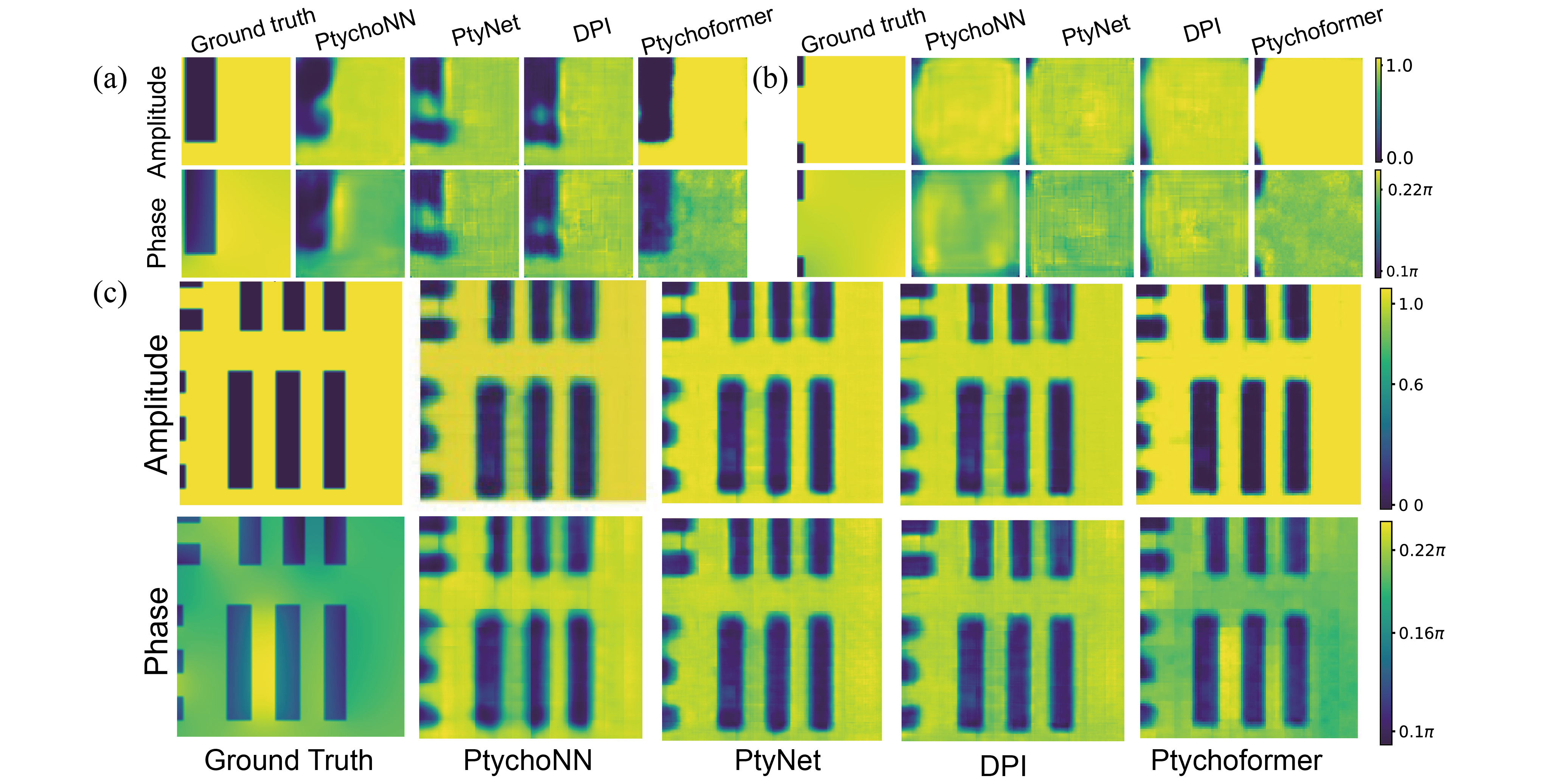
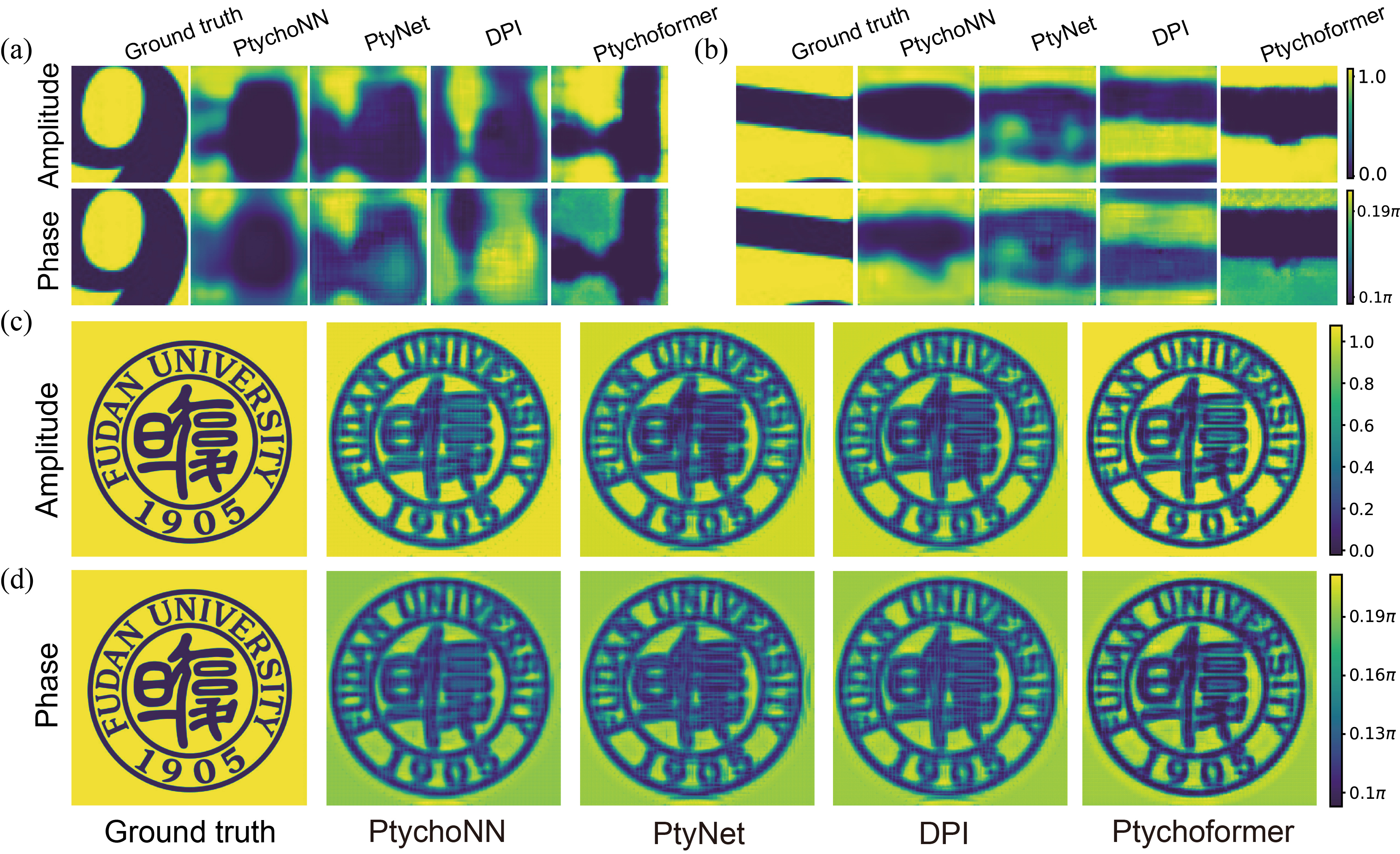
Ptychoformer produced retrievals with improved edge definition and clarity compared to those from the other methods, particularly evident in the vertical edge on the left side of Fig. 4(a). The reconstructed images also showed contrast levels closer to the ground truth, with more natural transitions between dark and bright areas. By contrast, the CNN-based models tended to smooth these sharp features and introducing artifacts and distortions.

IV-B2 Full-stitched Field Retrieval Analysis

Table I presents full-field stitching results under ideal (noise-free) and realistic (noisy) conditions, demonstrating Ptychoformer’s superior performance across all metrics. In ideal conditions, Ptychoformer achieved 16.0% lower MSE_amp and 6.7% higher PSNR_amp compared to PtychoNN, with similar improvements under noisy conditions. Fig. 4(c) visually confirms Ptychoformer’s superior global consistency and minimal boundary artifacts, particularly in reconstructing vertical column ends and background textures. The dual-branch structure enables our model to effectively capture both low-frequency and mid-to-high frequency information of diffraction patterns. This capability stems from the model’s ability to capture the intrinsic geometric structure of the data, analogous to continuous mapping on high-dimensional manifolds.

Repeated measures ANOVA and pairwise $t$-tests (Bonferroni correction, $\alpha=0.0083$) showed Ptychoformer significantly outperformed the other methods in all metrics in both conditions ($p<0.0083$), especially in MSE_amp and SSIM_amp ($p<0.0001$). The three CNN-based methods showed no significant differences, performing similarly across most metrics.

IV-C Validation on Experimental Synchrotron Data

Figure 5: Performance comparison on real experimental samples. (a,b) Visual comparison of retrieved amplitude and phase. For a specific hook-shaped detail, only our model effectively restores it, significantly outperforming CNN-based methods in fine structure retrieval. (c-e) Quantitative comparison of PSNR, SSIM, and MSE.

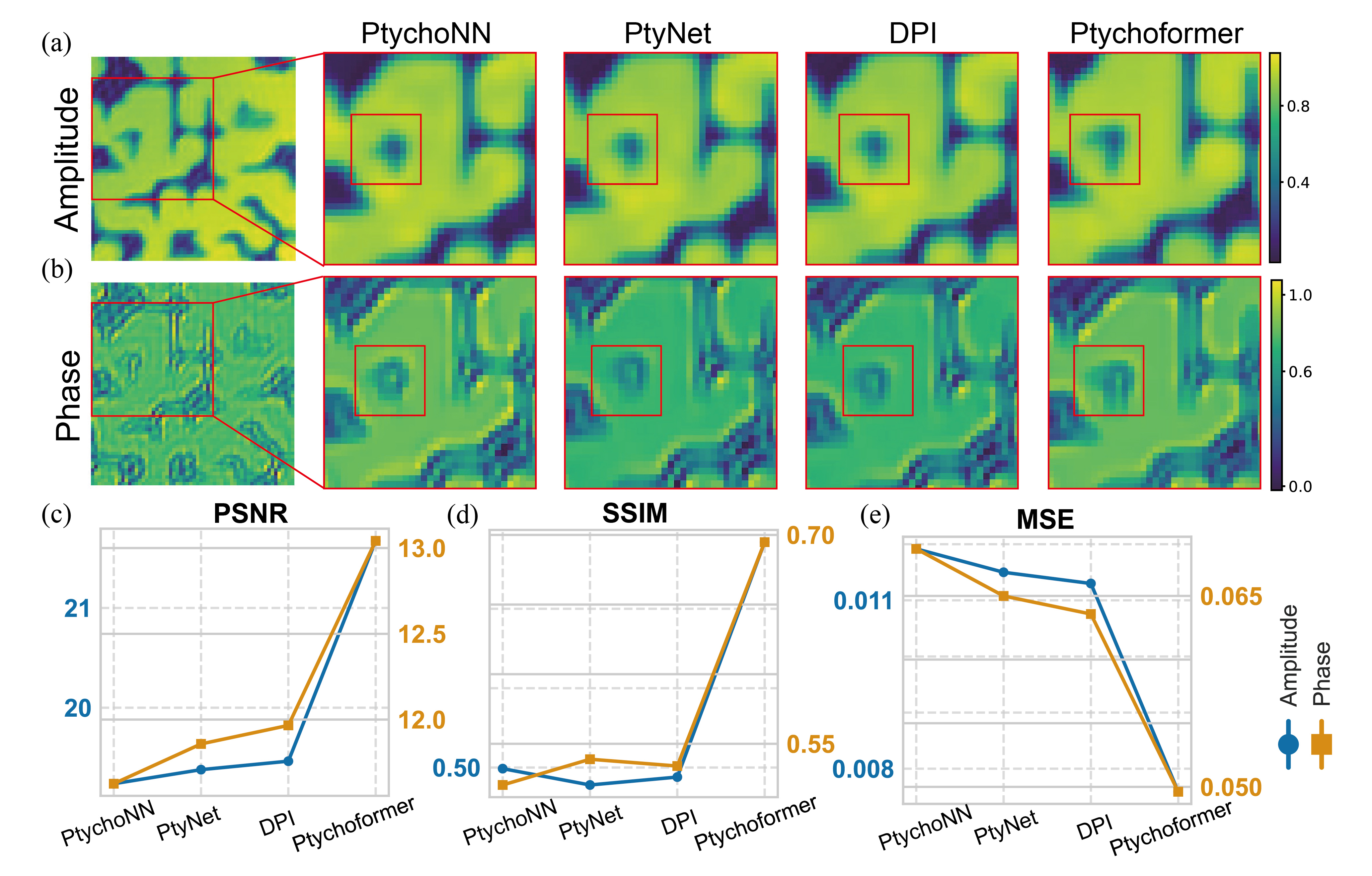
Fig. 5 demonstrates Ptychoformer’s superior performance on real experimental data, consistent with our findings from simulated datasets. Across all metrics (PSNR, SSIM, and MSE) for both amplitude and phase retrieval, Ptychoformer consistently outperforms other models. These improvements are visible in fine structural details (Fig. 5a,b), indicating Ptychoformer’s enhanced resolution and fidelity in practical imaging applications.

IV-D Generalization Capabilities Comparison

We evaluated Ptychoformer’s generalization by trained on simulated tungsten patterns with straight-line features and evaluated on complex, curved patterns without fine-tuning, assessing the model’s ability to extrapolate learned features to significantly different sample geometries. Fig. 6 shows Ptychoformer’s superior retrieval of curved patterns. Quantitative results in Table II support these visual observations. For amplitude retrieval, Ptychoformer achieves a PSNR_amp of 8.92 dB and SSIM_amp of 59.06%, outperforming other models by 0.83-0.95 dB and 8.51-11.28%, respectively. For phase retrieval, Ptychoformer attains a PSNR_phase of 8.68 dB and SSIM_phase of 49.44%, surpassing other models by 0.91-1.04 dB and 32.16-35.71%, respectively. These results demonstrate Ptychoformer’s ability to capture fundamental relationships between diffraction patterns and sample structures, aligning with the geometry-agnostic nature of ptychographic phase retrieval.

Figure 6: Comparison of generalization capabilities across different models: Direct test on a new unseen sample with significantly different distribution from the training set. (a) Amplitude and (b) phase retrieval of a single diffraction pattern. (c) Amplitude and (d) phase retrieval of a full scene (Fudan University logo). Models compared: Ground truth, PtychoNN, PtyNet, DPI, and Ptychoformer.

TABLE II: Performance Comparison for Out-of-Distribution Generalization.

Model	Amplitude		Phase
	PSNR (dB)	SSIM (%)	PSNR (dB)	SSIM (%)
PtychoNN	8.03	50.55	7.77	37.34
PtyNet	7.97	47.78	7.64	36.43
DPI	8.09	50.14	7.65	37.41
Ptychoformer	8.92	59.06	8.68	49.44

IV-E Performance Comparison Under Limited Data

Despite significant advancements in ptychography, a major challenge remains: extended data acquisition periods. While higher overlap between scanning points typically yields better retrieval results [14], it also increases experiment duration and radiation exposure. This is particularly problematic for radiation-sensitive materials [30] and in situ dynamic studies [31]. Our study focuses on this aspect, evaluating model performance under two kinds of limited data conditions.

IV-E1 Impact of Training Set Size

Figure 7: Training and testing set divisions of different sizes. Black boxes represent training set sizes, while white boxes represent testing sets, shown as squares.

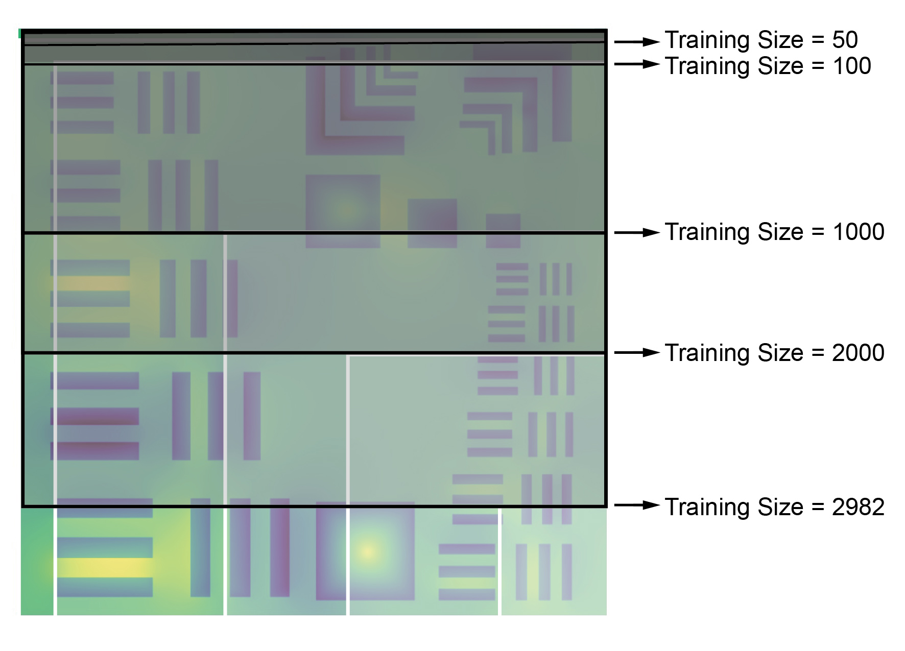
Fig. 8 (a-c) illustrates Ptychoformer’s performance under varying training set sizes. As the training size decreases from 2928 to 50, Ptychoformer consistently outperforms CNN-based models, especially at smaller training set sizes. Comparing with DPI, the best-performing CNN method, we showcase results at representative training sizes of 1000 and 50. Even with 1000 samples, DPI exhibits limitations with complex structures like the top-right crosshatch pattern, producing block-shaped high-frequency artifacts. Ptychoformer, in contrast, maintains superior resolution. At the minimal training size of 50 samples, DPI’s retrieval quality significantly deteriorates, while Ptychoformer still distinguishes basic structural features like crosshatches and L-shaped patterns. This robustness is attributed to Ptychoformer’s PCA mechanism and dual-branch architecture, which align with diffraction physics and capture multi-scale features effectively, demonstrating superior ability to learn from limited data.

IV-E2 Performance Across Overlap Ratios

Fig. 8 (d) demonstrates Ptychoformer’s effectiveness at varying overlap ratios. At 0% overlap, Ptychoformer achieves higher PSNR_amp, surpassing CNNs. From 75% to 0% overlap, Ptychoformer’s PSNR_amp drops by a smaller amount compared to CNNs. This resilience, analyzable through compressed sensing theory. [32], suggests Ptychoformer learns an optimal sparse prior. Lower overlap requirements could enable faster experiments with reduced radiation damage. Ptychoformer’s efficiency demonstrates the synergy between deep learning and domain-specific knowledge in ptychography.

Figure 8: Performance comparison across training set sizes and overlap ratios. (a,b) Retrievals with 1000 and 50 training samples. (c,d) PSNR and SSIM metrics for varying training sizes and overlap ratios. Higher values for both PSNR and SSIM indicate better performance.

TABLE III: Ablation Study Results

Model Variant	Amplitude		Phase
	PSNR (dB)	SSIM (%)	PSNR (dB)	SSIM (%)
Ours w/o NLB	14.10	86.60	18.39	65.40
Ours w/ MinN	13.82	83.90	18.64	64.10
Ours w/o D	11.02	60.50	17.32	54.50
Ours w/o OC	14.21	86.10	18.39	69.40
Ours	14.42	87.00	19.41	70.60

IV-F Ablation Study

To justify each component of the proposed Ptychoformer, we conducted comprehensive ablation studies. We compared several variants of our model: 1) Ours without NonLocal Coherence Branch (Ours w/o NLB), using only the Local Dependencies Branch; 2) Ours with Multi-Head Self-Attention (MHSA) in NLB (Ours w/ MinN), replacing PCA with standard MHSA in the NonLocal Branch; 3) Ours without Decoder (Ours w/o D), using fully connected layers instead of CNN for upsampling in the decoder; 4) Ours without Output Constraints (Ours w/o OC), removing the amplitude and phase constraints in the output layer; and 5) Ours (Full Model), the complete proposed Ptychoformer model. Table III presents the quantitative results of these variants, with the best performance in bold. The NonLocal Coherence Branch, reflecting diffraction patterns’ global nature, showed a modest impact, primarily affecting structural integrity. PCA demonstrated clear advantages over standard MHSA, with its replacement by MHSA causing a 4.16% drop in PSNR_amp and 3.56% in SSIM_amp.

The CNN decoder proved crucial, its absence leading to a substantial 23.58% decrease in PSNR_amp and 30.46% in SSIM_amp. This significant impact is attributed not only to its role in maintaining spatial coherence during upsampling but also to its inductive bias, which enables effective learning from limited data. Output constraints, while showing a modest quantitative impact, play a vital role in enforcing physical consistency. These results validate the effectiveness of each proposed component in our architecture.

V Discussion

V-A Frequency Analysis

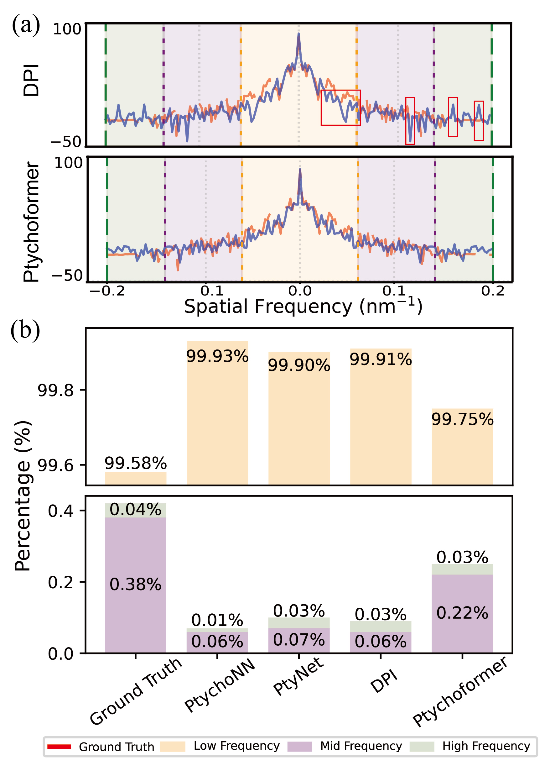
Further analysis of the noise-free full-stitched field using 1D diagonal cross-sections of the average 2D power spectral density (PSD) and frequency distribution statistics (Fig. 9). In Fig. 9(a), Ptychoformer’s PSD curve closely follows the ground truth, while the DPI model exhibits significant mid and high-frequency fluctuations, indicating potential artifacts. Quantitatively, Ptychoformer achieves a frequency distribution (99.75%, 0.22%, 0.03% for low, mid, and high frequencies, respectively), closely approximating the ground truth (99.58%, 0.38%, 0.04%). This performance exceeds that of CNN-based models, which show mid and high frequency degradation (e.g., PtychoNN: 99.93%, 0.06%, 0.01%). These results highlight Ptychoformer’s efficacy in extracting mid-to-high frequency information and retrieving corresponding detailed features, leading to superior artifact suppression.

Figure 9: Frequency analysis comparison of full-scene ptychographic retrievals. (a) 1D diagonal cross-sections of average 2D PSD from stitched simulations. Red curve: ground truth; Blue curve: models. The red box represents obvious abnormal model retrieval. (b) Quantitative breakdown of energy distribution across low, mid, and high frequency bands. Frequency ranges are defined based on the radial distance from the PSD center, with boundaries at 1/3 and 2/3 of the maximum frequency.

Figure 10: Performance analysis of weighted loss function $L_{\text{combined}}(\alpha)=\alpha L_{\text{MSE}}+(1-\alpha)L_{\text{NSSIM}}$ in ptychographic retrieval. PSNR, SSIM are plotted against $\alpha$ for amplitude and phase retrievals.

V-B Loss Function Analysis

To optimize retrieval quality in ptychographic phase retrieval, we evaluated various loss functions (as shown in Table IV. Standard metrics like MSE and Mean Absolute Error (MAE) showed similar performance, while the Huber loss [33], defined as: $L_{\text{Huber}}(x)=\begin{cases}\frac{1}{2}x^{2}&\text{for }|x|\leq\delta\\ \delta(|x|-\frac{1}{2}\delta)&\text{otherwise}\end{cases}$ offered robustness to outliers. The Negative Pearson Correlation Coefficient (NPCC) [34] loss, despite its success in single-frame phase retrieval [12], showed poor convergence stability in our experiments. This is likely due to its sensitivity to local statistics in small ptychographic patches, contrasting with its effectiveness on larger, more statistically stable single-frame images.

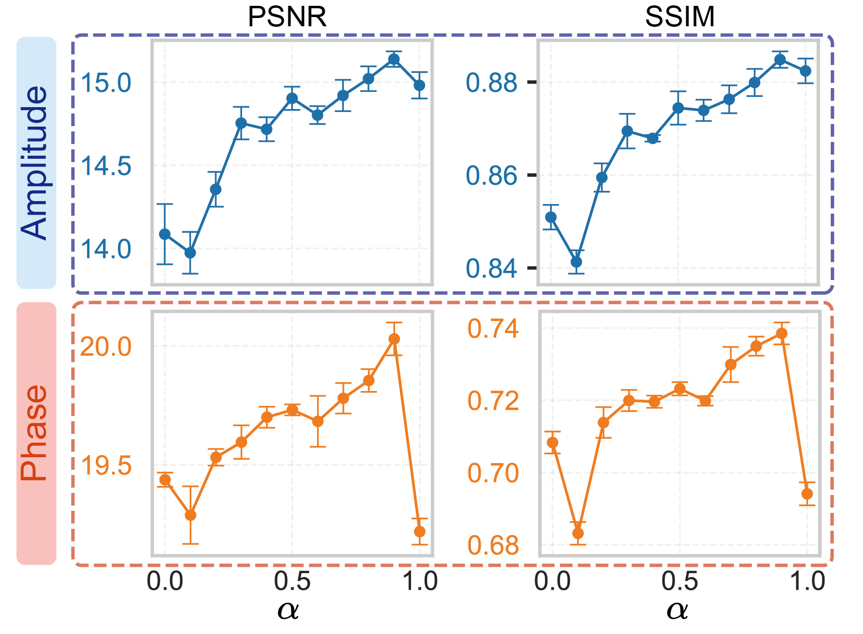
We introduced a novel combined loss function inspired by the work on image restoration with neural networks [35]: $L_{\text{combined}}(\alpha)=\alpha L_{\text{MSE}}+(1-\alpha)L_{\text{NSSIM}}$ where $L_{\text{NSSIM}}=-\text{SSIM}(I_{q},|\mathcal{F}{P(r)\psi(r)}|^{2})$, where $\psi(r)$ defined as $\psi(r)=P(r-r_{j})O(r)$. This approach balances global consistency (MSE) with local structural preservation ( Negative Structural Similarity Index Measure (NSSIM) [36]). Experiments revealed optimal performance at $\alpha=0.9$, with consistent improvement as $\alpha$ increased from 0.2 to 0.9, as shown in Fig. 10. This robustness to $\alpha$ values reduces the need for precise tuning in practical applications. The combined loss function excels in addressing affine ambiguity, as $\nabla L_{\text{MSE}}$ is sensitive to global affine transformations $T$ ($\frac{\partial L_{\text{MSE}}}{\partial T}\neq 0$), while $\nabla L_{\text{NSSIM}}$ maintains local structure invariance ($\frac{\partial L_{\text{NSSIM}}}{\partial(\text{local structure})}\approx 0$), forming a more robust optimization target.

TABLE IV: Comparison with Different Loss Functions

Loss Function	Amplitude		Phase
	PSNR (dB)	SSIM (%)	PSNR (dB)	SSIM (%)
MSE Loss	14.42	87.00	19.47	70.60
MAE Loss	13.63	85.90	19.29	67.50
Huber Loss	14.64	87.40	19.54	68.40
NPCC Loss	10.36	69.90	17.03	66.90
NSSIM Loss	14.12	85.10	19.41	70.80
Weighted Loss ($\alpha=0.9$)	15.10	88.50	20.04	73.90

Note:The weighted loss combines MSE and NSSIM losses, where $\alpha$ represents the weight of MSE (0.9) and 1-$\alpha$ (0.1) is the weight of NSSIM.

V-C Model Variants

To validate the effectiveness of our physics-informed design, we compared Ptychoformer with two state-of-the-art hybrid CNN-ViT models, adapted for ptychography task. The first is a TransUNet-inspired model [37], which uses a hybrid CNN-Transformer encoder where CNN extracts features and the Transformer processes them further. Its decoder employs a cascading structure with skip connections. The second is a SegFormer-based model [38], which features a hierarchical structure with progressive resolution reduction for multi-scale features. This model replaces the first linear layer in the feed-forward network with a $3\times 3$ convolution. We conducted the same experiment as in Section IV-B2 under noise-free conditions. Table V shows that Ptychoformer outperforms both models. TransUNet and SegFormer’s limitations stem from designs optimized for real-space image processing. The TransUNet variant, while benefiting from the combination of CNN and Transformer, still relies on local feature extraction in its initial stages. This approach is suboptimal for capturing the global coherence information present in diffraction patterns. Similarly, the SegFormer variant’s hierarchical structure, while effective for multi-scale feature extraction in natural images, may lose critical high-frequency information in the context of diffraction patterns due to its progressive downsampling.

TABLE V: Performance comparison of Model Variants.

Method	Amplitude		Phase
	PSNR (dB)	SSIM (%)	PSNR (dB)	SSIM (%)
TransUNet[37]	13.57	81.20	18.77	67.80
SegFormer[38]	13.76	83.30	19.12	68.10
Ptychoformer	14.42	87.00	19.41	70.60

VI Conclusion

In this study, we introduced Ptychoformer, a deep learning framework designed for ptychographic retrieval from frequency-domain data. By incorporating physical insights into the model architecture, particularly through the PCA mechanism and dual-branch structure, Ptychoformer demonstrated superior performance over existing state-of-the-art methods, particularly in high-frequency artifact suppression and data efficiency. The principles underlying Ptychoformer show promise for extension to other frequency-domain inverse imaging problems, potentially advancing high-resolution retrieval techniques across various scientific disciplines.

References

- [1] R. Hegerl and W. Hoppe, “Dynamische Theorie der Kristallstrukturanalyse durch Elektronenbeugung im inhomogenen Primärstrahlwellenfeld,” Ber Bunsenges Phys Chem, vol. 74, no. 11, pp. 1148–1154, Nov. 1970.
- [2] Y. Jiang, Z. Chen, Y. Han, P. Deb, H. Gao, S. Xie, P. Purohit, M. W. Tate, J. Park, and S. M. Gruner, “Electron ptychography of 2D materials to deep sub-ångström resolution,” Nature, vol. 559, no. 7714, pp. 343–349, 2018.
- [3] W. Yang, H. Sha, J. Cui, L. Mao, and R. Yu, “Local-orbital ptychography for ultrahigh-resolution imaging,” Nature Nanotechnology, pp. 1–6, 2024.
- [4] E. B. L. Pedersen, D. Angmo, H. F. Dam, K. T. S. Thydén, T. R. Andersen, E. T. B. Skjønsfjell, F. C. Krebs, M. Holler, A. Diaz, and M. Guizar-Sicairos, “Improving organic tandem solar cells based on water-processed nanoparticles by quantitative 3D nanoimaging,” Nanoscale, vol. 7, no. 32, pp. 13 765–13 774, 2015.
- [5] R. Kasprowicz, R. Suman, and P. O’Toole, “Characterising live cell behaviour: Traditional label-free and quantitative phase imaging approaches,” The international journal of biochemistry & cell biology, vol. 84, pp. 89–95, 2017.
- [6] M. Holler, M. Guizar-Sicairos, E. H. Tsai, R. Dinapoli, E. Müller, O. Bunk, J. Raabe, and G. Aeppli, “High-resolution non-destructive three-dimensional imaging of integrated circuits,” Nature, vol. 543, no. 7645, pp. 402–406, 2017.
- [7] A. V. Babu, T. Zhou, S. Kandel, T. Bicer, Z. Liu, W. Judge, D. J. Ching, Y. Jiang, S. Veseli, and S. Henke, “Deep learning at the edge enables real-time streaming ptychographic imaging,” Nature Communications, vol. 14, no. 1, p. 7059, 2023.
- [8] T. B. Edo, D. J. Batey, A. M. Maiden, C. Rau, U. Wagner, Z. D. Pešić, T. A. Waigh, and J. M. Rodenburg, “Sampling in x-ray ptychography,” Phys. Rev. A, vol. 87, no. 5, p. 053850, May 2013.
- [9] M. J. Cherukara, T. Zhou, Y. Nashed, P. Enfedaque, A. Hexemer, R. J. Harder, and M. V. Holt, “AI-enabled high-resolution scanning coherent diffraction imaging,” Applied Physics Letters, vol. 117, no. 4, 2020.
- [10] D. J. Chang, C. M. O’Leary, C. Su, D. A. Jacobs, S. Kahn, A. Zettl, J. Ciston, P. Ercius, and J. Miao, “Deep-Learning Electron Diffractive Imaging,” Phys. Rev. Lett., vol. 130, no. 1, p. 016101, Jan. 2023.
- [11] X. Pan, S. Wang, Z. Zhou, L. Zhou, P. Liu, C. Li, W. Wang, C. Zhang, Y. Dong, and Y. Zhang, “An efficient ptychography reconstruction strategy through fine-tuning of large pre-trained deep learning model,” Iscience, vol. 26, no. 12, 2023.
- [12] M. Deng, S. Li, A. Goy, I. Kang, and G. Barbastathis, “Learning to synthesize: Robust phase retrieval at low photon counts,” Light: Science & Applications, vol. 9, no. 1, p. 36, 2020.
- [13] R. Fan, J. Hao, R. Chen, J. Wang, Y. Lin, J. Jin, R. Yang, X. Zheng, K. Wang, and D. Lin, “Phase retrieval based on deep learning with bandpass filtering in holographic data storage,” Optics Express, vol. 32, no. 3, pp. 4498–4510, 2024.
- [14] P. M. Pelz, M. Guizar-Sicairos, P. Thibault, I. Johnson, M. Holler, and A. Menzel, “On-the-fly scans for X-ray ptychography,” Applied Physics Letters, vol. 105, no. 25, 2014.
- [15] J. Seifert, Y. Shao, and A. P. Mosk, “Noise-robust latent vector reconstruction in ptychography using deep generative models,” Optics Express, vol. 32, no. 1, pp. 1020–1033, 2024.
- [16] M. Du, X. Huang, and C. Jacobsen, “Using a modified double deep image prior for crosstalk mitigation in multislice ptychography,” Journal of synchrotron radiation, vol. 28, no. 4, pp. 1137–1145, 2021.
- [17] W. Gan, Q. Zhai, M. T. McCann, C. G. Cardona, U. S. Kamilov, and B. Wohlberg, “PtychoDV: Vision Transformer-Based Deep Unrolling Network for Ptychographic Image Reconstruction,” IEEE Open Journal of Signal Processing, 2024.
- [18] G. B. Parrent and B. J. Thompson, “On the Fraunhofer (Far Field) Diffraction Patterns of Opaque and Transparent Objects with Coherent Background,” Optica Acta: International Journal of Optics, vol. 11, no. 3, pp. 183–193, Jul. 1964.
- [19] J. Z. Buchwald and C.-P. Yeang, “Kirchhoff’s theory for optical diffraction, its predecessor and subsequent development: The resilience of an inconsistent theory,” Arch. Hist. Exact Sci., vol. 70, no. 5, pp. 463–511, Sep. 2016.
- [20] K. Simonyan and A. Zisserman, “Very Deep Convolutional Networks for Large-Scale Image Recognition,” Apr. 2015.
- [21] A. Krizhevsky, I. Sutskever, and G. E. Hinton, “Imagenet classification with deep convolutional neural networks,” Advances in neural information processing systems, vol. 25, 2012.
- [22] A. Dosovitskiy, L. Beyer, A. Kolesnikov, D. Weissenborn, X. Zhai, T. Unterthiner, M. Dehghani, M. Minderer, G. Heigold, S. Gelly, J. Uszkoreit, and N. Houlsby, “An Image is Worth 16x16 Words: Transformers for Image Recognition at Scale,” Jun. 2021.
- [23] Y. Yao, H. Chan, S. Sankaranarayanan, P. Balaprakash, R. J. Harder, and M. J. Cherukara, “AutoPhaseNN: Unsupervised physics-aware deep learning of 3D nanoscale Bragg coherent diffraction imaging,” npj Computational Materials, vol. 8, no. 1, p. 124, 2022.
- [24] Y. Li, C.-Y. Wu, H. Fan, K. Mangalam, B. Xiong, J. Malik, and C. Feichtenhofer, “Mvitv2: Improved multiscale vision transformers for classification and detection,” in Proceedings of the IEEE/CVF Conference on Computer Vision and Pattern Recognition, 2022, pp. 4804–4814.
- [25] K. Han, Y. Wang, H. Chen, X. Chen, J. Guo, Z. Liu, Y. Tang, A. Xiao, C. Xu, and Y. Xu, “A survey on vision transformer,” IEEE transactions on pattern analysis and machine intelligence, vol. 45, no. 1, pp. 87–110, 2022.
- [26] J. Wu, W. Ji, H. Fu, M. Xu, Y. Jin, and Y. Xu, “Medsegdiff-v2: Diffusion-based medical image segmentation with transformer,” in Proceedings of the AAAI Conference on Artificial Intelligence, vol. 38, 2024, pp. 6030–6038.
- [27] T. Nguyen, J. Jewik, H. Bansal, P. Sharma, and A. Grover, “Climatelearn: Benchmarking machine learning for weather and climate modeling,” Advances in Neural Information Processing Systems, vol. 36, 2024.
- [28] J. Chang and J. C. Ye, “Bidirectional generation of structure and properties through a single molecular foundation model,” Nature Communications, vol. 15, no. 1, p. 2323, 2024.
- [29] T. Zhou, M. Cherukara, and C. Phatak, “Differential programming enabled functional imaging with Lorentz transmission electron microscopy,” npj Computational Materials, vol. 7, no. 1, p. 141, 2021.
- [30] A. Bhartiya, D. Batey, S. Cipiccia, X. Shi, C. Rau, S. Botchway, M. Yusuf, and I. K. Robinson, “X-ray Ptychography Imaging of Human Chromosomes After Low-dose Irradiation,” Chromosome Res, vol. 29, no. 1, pp. 107–126, Mar. 2021.
- [31] J. N. Weker, X. Huang, and M. F. Toney, “In situ X-ray-based imaging of nano materials,” Current opinion in chemical engineering, vol. 12, pp. 14–21, 2016.
- [32] E. J. Candès, J. Romberg, and T. Tao, “Robust uncertainty principles: Exact signal reconstruction from highly incomplete frequency information,” IEEE Transactions on information theory, vol. 52, no. 2, pp. 489–509, 2006.
- [33] P. J. Huber, “Robust Estimation of a Location Parameter,” in Breakthroughs in Statistics, S. Kotz and N. L. Johnson, Eds. New York, NY: Springer New York, 1992, pp. 492–518.
- [34] “VII. Note on regression and inheritance in the case of two parents,” Proc. R. Soc. Lond., vol. 58, no. 347-352, pp. 240–242, Dec. 1895.
- [35] H. Zhao, O. Gallo, I. Frosio, and J. Kautz, “Loss functions for image restoration with neural networks,” IEEE Transactions on computational imaging, vol. 3, no. 1, pp. 47–57, 2016.
- [36] Z. Wang, A. C. Bovik, H. R. Sheikh, and E. P. Simoncelli, “Image quality assessment: From error visibility to structural similarity,” IEEE transactions on image processing, vol. 13, no. 4, pp. 600–612, 2004.
- [37] J. Chen, Y. Lu, Q. Yu, X. Luo, E. Adeli, Y. Wang, L. Lu, A. L. Yuille, and Y. Zhou, “TransUNet: Transformers Make Strong Encoders for Medical Image Segmentation,” Feb. 2021.
- [38] E. Xie, W. Wang, Z. Yu, A. Anandkumar, J. M. Alvarez, and P. Luo, “SegFormer: Simple and efficient design for semantic segmentation with transformers,” Advances in neural information processing systems, vol. 34, pp. 12 077–12 090, 2021.