Full-colour double-virtual amplitudes for associated production of a Higgs boson with a bottom-quark pair at the LHC

Abstract

We present the double-virtual amplitudes contributing to the production of a Higgs boson in association with a $b\bar{b}$ pair at the Large Hadron Collider. We perform the computation within the five-flavour scheme, which employs massless bottom quarks and finite bottom-Yukawa coupling, taking into account all the colour structures. We derive the analytic form of the helicity amplitudes through finite-field reconstruction techniques. The analytic expressions have been implemented in a public C++ library, and we demonstrate that evaluations are sufficiently stable and efficient for use in phenomenological studies.

1 Introduction

Studying the properties of the Higgs boson is one of the most important tasks in the programme of the Large Hadron Collider (LHC) following its discovery in 2012 ATLAS:2012yve ; CMS:2012qbp . Precision measurements of the Higgs boson coupling to other particles — such as top or bottom quark, $W$ or $Z$ boson — will improve our understanding of the Standard Model and might unveil deviations from it ATLAS:2022vkf ; CMS:2022dwd , especially in view of the vast amount of data collected from previous and current runs as well as those expected from the upcoming high-luminosity phase (HL-LHC) Cepeda:2019klc . The production of a Higgs boson in association with a bottom-quark pair at the LHC ($pp\to b\bar{b}H$) provides a direct access to probe the bottom-quark Yukawa coupling.

The fully inclusive cross section of $b\bar{b}H$ production at the LHC is comparable to that of Higgs production in association with a top-quark pair ($pp\to t\bar{t}H$), which comes after the gluon fusion channel ($pp(gg)\to H$), vector boson fusion ($pp\to qqH$) and $W/Z+H$ associated production LHCHiggsCrossSectionWorkingGroup:2016ypw . Imposing the $b$-jet identification to $b\bar{b}H$ production (by tagging either one or two $b$ jets) significantly decreases the production rate with respect to the inclusive case. In addition, large irreducible backgrounds may hinder the measurement of bottom-Yukawa coupling through the $b\bar{b}H$ production mechanism Pagani:2020rsg . Further studies to extract the $b\bar{b}H$ signal through its kinematic shape, as well as a proposal to probe non-standard $b\bar{b}H$ are available in the literature Grojean:2020ech ; Konar:2021nkk . The strength of the bottom-Yukawa coupling can be significantly amplified in models with modified Higgs sector, such as the Two Higgs Doublet Models (2HDM’s) and the Minimal Supersymmetric Standard Model (MSSM), resulting in the enhancement of the $b\bar{b}H$ production cross section Balazs:1998nt ; Dawson:2005vi . In addition to the possibility of constraining beyond-the-Standard-Model (BSM) scenarios that introduce a modification to the bottom-Yukawa coupling, $b\bar{b}H$ production also serves as an irreducible background for double Higgs production, where one of the Higgs boson decays into a bottom-quark pair. The accurate simulation of the $b\bar{b}H$ production will thus improve the measurement of the $pp\to HH$ cross section as well as the extraction of the triple Higgs coupling Manzoni:2023qaf . The first search for $b\bar{b}H$ production at the LHC has been carried out by the CMS collaboration using 13 TeV data with 138^-1 fb of integrated luminosity, setting an upper limit on the $b\bar{b}H$ total cross section CMS:2024eur .

Theoretical predictions for the $b\bar{b}H$ production can be obtained within either the five-flavour scheme (5FS) or the four-flavour scheme (4FS). In the 5FS, the bottom quark is treated as massless and can appear in the initial state. In the 4FS, instead, the bottom quark is treated as massive and is only allowed to appear in the final state. Owing to the vanishing of the bottom-quark mass, higher-order predictions are easier to obtain in the 5FS than in the 4FS. Indeed, theoretical predictions for inclusive $b\bar{b}H$ production in the 5FS ($pp(b\bar{b})\to H$) are available up to the Next-to-Next-to-Next-to-Leading Order (N3LO) in Quantum Chromodynamics (QCD) Dicus:1998hs ; Balazs:1998sb ; Maltoni:2003pn ; Harlander:2003ai ; Belyaev:2005bs ; Harlander:2010cz ; Ozeren:2010qp ; Buhler:2012ytl ; Harlander:2012pb ; Harlander:2014hya ; Ahmed:2014pka ; Gehrmann:2014vha ; AH:2019xds ; Duhr:2019kwi ; Mondini:2021nck , and matching to a parton shower (PS) has been carried out recently at Next-to-Next-to-Leading Order (NNLO) QCD accuracy Biello:2024vdh . In the case of one-tagged $b$ jet, the 5FS theoretical predictions have been considered by incorporating NLO QCD Campbell:2002zm , weak Dawson:2010yz , and supersymmetric QCD Dawson:2011pe corrections. On the other hand, the theoretical predictions in the 4FS are available up to Next-to-Leading Order (NLO) accuracy in QCD Dittmaier:2003ej ; Dawson:2003kb ; Dawson:2004sh , and in supersymmetric QCD Liu:2012qu ; Dittmaier:2014sva , including also, in addition to the bottom-quark Yukawa coupling, the contribution from the top-quark Yukawa coupling as well as their interferences Deutschmann:2018avk . 4FS NLO QCD predictions matched to parton shower are also available within the MC@NLO and Powheg matching schemes Wiesemann:2014ioa ; Jager:2015hka . We note that NNLO QCD prediction for $b\bar{b}W$ production and NNLO+PS prediction for $b\bar{b}Z$ production have been recently computed in the 4FS employing approximated two-loop amplitudes Buonocore:2022pqq ; Mazzitelli:2024ura , and the same computational strategies can be applied to the $b\bar{b}H$ process as well.

In this work, we compute analytically the two-loop five-particle scattering amplitudes contributing to $pp\to b\bar{b}H$ production in the 5FS, retaining the complete colour structure. These amplitudes are required in the NNLO QCD computation of $b\bar{b}H$ production where the two bottom quarks are identified. In the case of only one tagged bottom quark, instead, they contribute at N3LO QCD accuracy. Finally, for inclusive $b\bar{b}H$ production, they appear in the (Next-to-)⁴-Leading Order (N4LO) QCD calculation. This work extends the previous result where the two-loop five-particle amplitudes for $b\bar{b}H$ production were derived in the leading colour approximation Badger:2021ega .

The computation of two-loop five-point amplitudes has drawn huge interest in the past few years, since in most cases it is the main bottleneck in obtaining NNLO QCD prediction for $2\to 3$ scattering processes at the LHC. Impressive progress was made in this context, owing to several insights. Firstly, the advancement in the calculation of the required Feynman integrals using the differential equation method Gehrmann:2015bfy ; Papadopoulos:2015jft ; Abreu:2018rcw ; Chicherin:2018mue ; Chicherin:2018old ; Abreu:2018aqd ; Abreu:2020jxa ; Canko:2020ylt ; Abreu:2021smk ; Kardos:2022tpo ; Abreu:2023rco led to the construction of bases of special functions called pentagon functions Gehrmann:2018yef ; Chicherin:2020oor ; Chicherin:2021dyp ; Abreu:2023rco , which can be evaluated efficiently and which allow for an efficient computation of the amplitudes. Secondly, the use of finite-field arithmetic has proven to be critical in tackling the algebraic complexity of multi-particle amplitudes vonManteuffel:2014ixa ; Peraro:2016wsq ; Klappert:2019emp ; Peraro:2019svx ; Klappert:2020aqs ; Klappert:2020nbg . Finally, new techniques to obtain optimised systems of integration-by-part (IBP) relations further reduced one of the main bottlenecks in the computation of scattering amplitudes (see for example Refs. Gluza:2010ws ; Schabinger:2011dz ; Ita:2015tya ; Chen:2015lyz ; Bohm:2017qme ; Bosma:2018mtf ; Boehm:2020zig ; Guan:2024byi ; Chestnov:2024mnw ). Thanks to all these developments, full colour two-loop analytic results Badger:2019djh ; Agarwal:2021vdh ; Badger:2021imn ; Abreu:2023bdp ; Badger:2023mgf ; Agarwal:2023suw ; DeLaurentis:2023nss ; DeLaurentis:2023izi are now available for all massless five-particle scattering processes of interest for the LHC, superseding the leading colour results Gehrmann:2015bfy ; Badger:2018enw ; Abreu:2018zmy ; Abreu:2019odu ; Abreu:2020cwb ; Chawdhry:2020for ; Agarwal:2021grm ; Chawdhry:2021mkw ; Abreu:2021oya . In the case of two-loop five-particle amplitudes with an external mass, instead, analytic expressions are only available in the leading colour approximation Badger:2021nhg ; Badger:2021ega ; Abreu:2021asb ; Badger:2022ncb , although the full set of master integrals have been computed. Full colour results for a process of this class have been recently obtained for $W\gamma\gamma$ production at the LHC, with the subleading colour contributions taken into account numerically Badger:2024sqv . The availability of compact analytic results for two-loop five-point amplitudes, together with a stable and efficient routine for the numerical evaluation of the pentagon functions PentagonFunctions:cpp , have enabled several NNLO QCD calculations for $2\to 3$ scattering processes Chawdhry:2019bji ; Kallweit:2020gcp ; Chawdhry:2021hkp ; Czakon:2021mjy ; Badger:2021ohm ; Chen:2022ktf ; Alvarez:2023fhi ; Badger:2023mgf ; Hartanto:2022qhh ; Hartanto:2022ypo ; Buonocore:2022pqq ; Catani:2022mfv ; Buonocore:2023ljm ; Mazzitelli:2024ura ; Devoto:2024nhl . The result presented in this work is the first analytic full colour amplitude for a two-loop five-point scattering process with an external mass.

Although efforts to include more external or internal masses, or even more external legs, have recently been made Henn:2021cyv ; Badger:2022hno ; FebresCordero:2023pww ; Agarwal:2024jyq ; Henn:2024ngj ; Badger:2024fgb ; Jiang:2024eaj ; Abreu:2024yit , computing NNLO QCD predictions for $b\bar{b}H$ production in the 4FS with exact two-loop matrix elements remains out of reach of current amplitude technology. However, given that the bottom-quark mass ($m_{b}$) is the smallest scale in the process, a good approximation of the 4FS prediction may still be obtained by restoring the leading $m_{b}$ contributions through the massification prescription Mitov:2006xs starting from our massless-$b$ results. Indeed, in the context of $2\to 3$ processes, this approach has already been adopted successfully to $pp\to b\bar{b}W$ and $pp\to b\bar{b}Z$ Buonocore:2022pqq ; Mazzitelli:2024ura .

Our paper is organised as follows. In Section 2, we discuss the full colour structure of the partonic amplitudes together with the definition of the finite remainders. Section 3 is devoted to our computational strategy, starting from how we defined the helicity amplitudes, followed by a discussion of our finite-field framework. We present a benchmark numerical evaluation at a physical phase-space point, describe the C++ implementation and examine the numerical stability of our amplitude in Section 4. We finally draw our conclusion in Section 5.

2 Structure of the amplitudes

We compute the two-loop five-particle helicity amplitudes contributing to $b\bar{b}H$ production at hadron colliders in the 5FS. At partonic level, there is a single two-quark two-gluon scattering process

$$0\rightarrow\bar{b}(p_{1})+b(p_{2})+g(p_{3})+g(p_{4})+H(p_{5})\,,$$ (1)

and two four-quark scattering processes

$$0\rightarrow\bar{b}(p_{1})+b(p_{2})+\bar{q}(p_{3})+q(p_{4})+H(p_{5})\,,$$ (2)

$$0\rightarrow\bar{b}(p_{1})+b(p_{2})+\bar{b}(p_{3})+b(p_{4})+H(p_{5})\,.$$ (3)

In this section we first define our parametrisation of the kinematics. Next, we describe the structure of the two-loop amplitudes for these classes of partonic process. We then discuss the construction of finite remainders, obtained by subtracting the ultraviolet (UV) and infrared (IR) singularities from the bare amplitudes. Finally, we give the explicit dependence of the finite remainders on the renormalisation scale.

2.1 Kinematics

We work in the ’t Hooft-Veltman (HV) scheme with $d=4-2\epsilon$ space-time dimensions and four-dimensional external momenta $p_{i}$. The latter are taken to be all outgoing, and satisfy momentum conservation,

$$\sum_{i=1}^{5}p_{i}=0\,,$$ (4)

as well as the following on-shell conditions:

$$\begin{aligned} p_{i}^{2}&=0\quad\forall\;i=1,\dots,4\,,\\ p_{5}^{2}&=m_{H}^{2}\,,\end{aligned}$$ (5)

where $m_{H}$ is the Higgs boson mass. Although the bottom-quark mass is set to zero in Eq. (5), as required in the 5FS, the bottom-quark Yukawa coupling is kept finite Harlander:2003ai ; Duhr:2019kwi ; Mondini:2021nck . We choose the following six independent Mandelstam invariants,

$$\vec{s}=\{s_{12},s_{23},s_{34},s_{45},s_{15},m_{H}^{2}\}\,,$$ (6)

where $s_{ij\cdots k}=(p_{i}+p_{j}+\cdots+p_{k})^{2}$. Together with the following parity-odd invariant,

$$\operatorname{\rm tr}_{5}=4\,\mathrm{i}\,\varepsilon_{\mu\nu\rho\sigma}\,p_{1}^{\mu}p_{2}^{\nu}p_{3}^{\rho}p_{4}^{\sigma}\,,$$ (7)

where $\varepsilon_{\mu\nu\rho\sigma}$ is the anti-symmetric Levi-Civita pseudo-tensor, they fully describe the five-particle kinematics in the presence of an external mass.

While the sign of $\operatorname{\rm tr}_{5}$ captures the parity degree of freedom of the helicity amplitudes, $\operatorname{\rm tr}_{5}^{2}\equiv\Delta_{5}$ is a degree-4 irreducible polynomial in the Mandelstam invariants $\vec{s}$. The parametrisation of the kinematics in terms of $\vec{s}$ therefore contains the square root of $\Delta_{5}$. For the computation of the helicity amplitudes, we prefer to adopt a parametrisation of the kinematics in terms of momentum-twistor variables Hodges:2009hk ; Badger:2016uuq , which rationalises $\sqrt{\Delta_{5}}$ and the spinor-helicity brackets $\langle ij\rangle$ and $[ij]$ using a minimal set of variables (see e.g. Ref. Badger:2023eqz for an introduction).

In particular, we employ the parametrisation of Ref. Badger:2021ega . The Mandelstam invariants $\vec{s}$ are expressed in terms of the momentum-twistor variables $\vec{x}=\{x_{1},\ldots,x_{6}\}$ as

$$\begin{aligned} s_{12}&=x_{1}\,,\\ s_{23}&=x_{1}x_{4}\,,\\ s_{34}&=x_{1}\left[\frac{(1+x_{3})x_{4}}{x_{2}}-x_{3}\Bigl{(}1+x_{4}(x_{5}-1)\Bigr{)}\right]\,,\\ s_{45}&=x_{1}x_{6}\,,\\ s_{15}&=x_{1}x_{3}(x_{2}-x_{4}x_{5})\,,\\ m_{H}^{2}&=\frac{x_{1}x_{3}}{x_{4}}(x_{2}-x_{4})\Bigl{[}x_{4}(x_{5}-1)+x_{6}\Bigr{]}\,.\end{aligned}$$ (8)

Conversely, the expression of the momentum-twistor variables in terms of momenta requires also the parity degree of freedom, which is captured by Dirac traces with $\gamma_{5}$:

$$x_{1}=s_{12}\,,\qquad x_{2}=-\frac{\operatorname{\rm tr}_{+}(1234)}{s_{12}s_{34}}\,,$$ (9)

$$x_{3}=\frac{\operatorname{\rm tr}_{+}[134152]}{s_{13}\operatorname{\rm tr}_{+}{[1452]}}\,,\qquad x_{4}=\frac{s_{23}}{s_{12}}\,,$$

$$x_{5}=-\frac{\operatorname{\rm tr}_{-}[1(2+3)(1+5)523]}{s_{23}\operatorname{\rm tr}_{-}[1523]}\,,\qquad x_{6}=\frac{s_{123}}{s_{12}}\,,$$

where

$$\operatorname{\rm tr}_{\pm}(ij\cdots kl)=\frac{1}{2}\operatorname{\rm tr}\left[(1\pm\gamma_{5})\not{p}_{i}\not{p}_{j}\cdots\not{p}_{k}\not{p}_{l}\right]\,,$$ (10)

$$\operatorname{\rm tr}_{\pm}[\cdots(i+j)\cdots]=\operatorname{\rm tr}_{\pm}(\cdots i\cdots)+\operatorname{\rm tr}_{\pm}(\cdots j\cdots)\,.$$ (11)

2.2 Two-quark two-gluon scattering channel

The colour decomposition of the $L$-loop amplitude $\mathcal{M}^{(L)}$ for the $0\to\bar{b}bggH$ channel is given by

$$\begin{aligned} \mathcal{M}^{(L)}(1_{\bar{b}},2_{b},3_{g},4_{g},5_{H})=\;&n^{L}\bar{g}_{s}^{2}\bar{y}_{b}\;\bigg{\{}(t^{a_{3}}t^{a_{4}})_{i_{2}}^{\;\;\bar{i}_{1}}\mathcal{A}^{(L)}_{34}(1_{\bar{b}},2_{b},3_{g},4_{g},5_{H})\\ &+(t^{a_{4}}t^{a_{3}})_{i_{2}}^{\;\;\bar{i}_{1}}\mathcal{A}^{(L)}_{43}(1_{\bar{b}},2_{b},3_{g},4_{g},5_{H})+\delta_{i_{2}}^{\;\;\bar{i}_{1}}\delta^{a_{3}a_{4}}\mathcal{A}^{(L)}_{\delta}(1_{\bar{b}},2_{b},3_{g},4_{g},5_{H})\bigg{\}}\,,\end{aligned}$$ (12)

where $n=(4\pi)^{\epsilon}e^{-\epsilon\gamma_{E}}\,\bar{\alpha}_{s}/(4\pi)$, $\bar{\alpha}_{s}=\bar{g}_{s}^{2}/(4\pi)$, $\bar{g}_{s}$ is the bare strong coupling constant, $\bar{y}_{b}$ is the bare bottom-Yukawa coupling, and $t^{a}$ are the $SU(N_{c})$ fundamental generators satisfying $\operatorname{\rm tr}(t^{a}t^{b})=\delta^{ab}/2$. The $\mathcal{A}^{(L)}_{43}$ partial amplitudes can be obtained from the $\mathcal{A}^{(L)}_{34}$ ones through

$$\mathcal{A}^{(L)}_{43}(1_{\bar{b}},2_{b},3_{g},4_{g},5_{H})=\mathcal{A}^{(L)}_{34}(1_{\bar{b}},2_{b},4_{g},3_{g},5_{H})\,.$$ (13)

We thus compute only $\mathcal{A}^{(L)}_{34}$ and $\mathcal{A}^{(L)}_{\delta}$. We further note that $\mathcal{A}^{(L)}_{\delta}$ vanishes at tree level.

The partial amplitudes are decomposed in terms of the number of colours ($N_{c}$) and the number of light quark flavours ($n_{f}$) appearing in closed massless quark loops. The $(N_{c},n_{f})$ decomposition of the one-loop partial amplitudes is given by

$$\mathcal{A}^{(1)}_{34} =N_{c}A^{(1),N_{c}}_{34}+\frac{1}{N_{c}}A^{(1),1/N_{c}}_{34}+n_{f}A^{(1),n_{f}}_{34}\,,$$ (14a)

$$\mathcal{A}^{(1)}_{\delta} =A^{(1),1}_{\delta}\,,$$ (14b)

while at two loops we have

$$\mathcal{A}^{(2)}_{34} =N_{c}^{2}A^{(2),N_{c}^{2}}_{34}+A^{(2),1}_{34}+\frac{1}{N_{c}^{2}}A^{(2),1/N_{c}^{2}}_{34}+N_{c}n_{f}A^{(2),N_{c}n_{f}}_{34}+\frac{n_{f}}{N_{c}}A^{(2),n_{f}/N_{c}}_{34}+n_{f}^{2}A^{(2),n_{f}^{2}}_{34}\,,$$ (15a)

$$\mathcal{A}^{(2)}_{\delta} =N_{c}A^{(2),N_{c}}_{\delta}+\frac{1}{N_{c}}A^{(2),1/N_{c}}_{\delta}+n_{f}A^{(2),n_{f}}_{\delta}+\frac{n_{f}}{N_{c}^{2}}A^{(2),n_{f}/N_{c}^{2}}_{\delta}\,.$$ (15b)

Representative two-loop Feynman diagrams together with the partial amplitudes they contribute to are shown in Fig. 1.

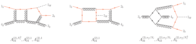
Figure 1: Representative two-loop Feynman diagrams appearing in the $0\to\bar{b}bggH$ scattering process, together with the partial amplitudes associated with each of the diagrams. Dashed lines denote the Higgs boson, while solid lines denote massless quarks (red for the bottom quark).

There are 8 distinct helicity configurations, of which 3 are independent and have been chosen as

$$\begin{aligned} \mathcal{M}^{(L)}(1_{\bar{b}}^{+},2_{b}^{+},3_{g}^{+},4_{g}^{+},5_{H})\,,\\ \mathcal{M}^{(L)}(1_{\bar{b}}^{+},2_{b}^{+},3_{g}^{+},4_{g}^{-},5_{H})\,,\\ \mathcal{M}^{(L)}(1_{\bar{b}}^{+},2_{b}^{+},3_{g}^{-},4_{g}^{-},5_{H})\,.\end{aligned}$$ (16)

We obtain the full set of partial amplitudes and helicity configurations from the independent ones by means of permutations of the external legs as well as parity conjugation. Since the momentum-twistor parametrisation of the kinematics fixes all spinor phases in order to minimise the number of independent variables, the phase information has to be restored before permutations or parity conjugation can be carried out. For this purpose, we employ the following phase factors:

$$\Phi_{\bar{b}bggH}^{++++} =\frac{s_{12}}{\langle 23\rangle\langle 34\rangle\langle 41\rangle}\,,$$ (17a)

$$\Phi_{\bar{b}bggH}^{+++-} =\frac{[13]^{2}}{[14][34]\langle 23\rangle}\,,$$ (17b)

$$\Phi_{\bar{b}bggH}^{++--} =\frac{[12]^{2}}{[23][34][41]}\,.$$ (17c)

We refer to Appendix C of Ref. Badger:2023mgf for a thorough discussion of how to permute and conjugate expressions in terms of momentum-twistor variables.

2.3 Four-quark scattering channel

For this class of partonic processes we first focus on the case involving two distinct quark flavours: a bottom quark and a massless quark $q\in\{u,d,c,s\}$. The colour decomposition of the $L$-loop amplitude $\mathcal{M}^{(L)}$ for the $0\to\bar{b}b\bar{q}qH$ channel is given by

$$\begin{aligned} \mathcal{M}^{(L)}(1_{\bar{b}},2_{b},3_{\bar{q}},4_{q},5_{H})=\;n^{L}\bar{g}_{s}^{2}\bar{y}_{b}\;\bigg{\{}&\delta_{i_{4}}^{\;\;\bar{i}_{1}}\delta_{i_{2}}^{\;\;\bar{i}_{3}}\,\mathcal{A}^{(L)}_{1}(1_{\bar{b}},2_{b},3_{\bar{q}},4_{q},5_{H})\\ &+\frac{1}{N_{c}}\delta_{i_{2}}^{\;\;\bar{i}_{1}}\delta_{i_{4}}^{\;\;\bar{i}_{3}}\,\mathcal{A}^{(L)}_{2}(1_{\bar{b}},2_{b},3_{\bar{q}},4_{q},5_{H})\bigg{\}}\,.\end{aligned}$$ (18)

Only one partial amplitude is independent at the tree level, since

$$\mathcal{A}^{(0)}_{2}(1_{\bar{b}},2_{b},3_{\bar{q}},4_{q},5_{H})=-\mathcal{A}^{(0)}_{1}(1_{\bar{b}},2_{b},3_{\bar{q}},4_{q},5_{H})\,.$$

At higher loop order we instead have to compute both $\mathcal{A}^{(L)}_{1}$ and $\mathcal{A}^{(L)}_{2}$. Their $(N_{c},n_{f})$ decomposition at one and two loops is given by

$$\mathcal{A}^{(1)}_{z} =N_{c}A^{(1),N_{c}}_{z}+\frac{1}{N_{c}}A^{(1),1/N_{c}}_{z}+n_{f}A^{(1),n_{f}}_{z}\,,$$ (19a)

$$\mathcal{A}^{(2)}_{z} =N_{c}^{2}A^{(2),N_{c}^{2}}_{z}+A^{(2),1}_{z}+\frac{1}{N_{c}^{2}}A^{(2),1/N_{c}^{2}}_{z}+N_{c}n_{f}A^{(2),N_{c}n_{f}}_{z}+\frac{n_{f}}{N_{c}}A^{(2),n_{f}/N_{c}}_{z}+n_{f}^{2}A^{(2),n_{f}^{2}}_{z}\,,$$ (19b)

where $z\in\{1,2\}$. Sample two-loop Feynman diagrams for the $0\to\bar{b}b\bar{q}qH$ scattering process are depicted in Fig. 2 together with the partial amplitudes they contribute to.

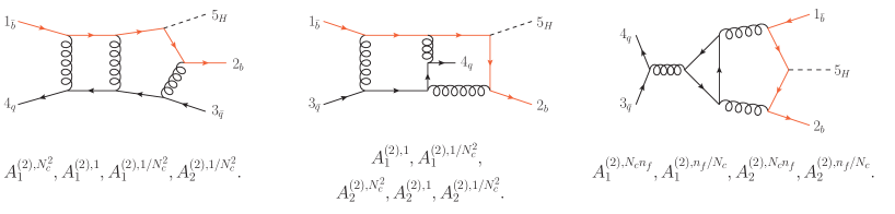
Figure 2: Representative two-loop Feynman diagrams appearing in the $0\to\bar{b}b\bar{q}qH$ scattering process, together with the partial amplitudes they contribute to. The notation is the same as in Fig. 1.

From the 4 contributing helicity configurations, only one is independent and was chosen to be

$$\mathcal{M}^{(L)}(1_{\bar{b}}^{+},2_{b}^{+},3_{\bar{q}}^{+},4_{q}^{-},5_{H}).$$ (20)

The corresponding spinor phase factor is

$$\Phi_{\bar{b}b\bar{q}qH}^{+++-} =\frac{\langle 42\rangle}{\langle 12\rangle\langle 23\rangle}\,.$$ (21)

We now extend the discussion to the four-quark scattering process involving two bottom-quark pairs: $0\to\bar{b}b\bar{b}bH$. In this case, the $L$-loop colour decomposition is given by

$$\begin{aligned} \mathcal{M}^{(L)}(1_{\bar{b}},2_{b},3_{\bar{b}},4_{b},5_{H})=\;n^{L}\bar{g}_{s}^{2}\bar{y}_{b}\;\bigg{\{}&\delta_{i_{4}}^{\;\;\bar{i}_{1}}\delta_{i_{2}}^{\;\;\bar{i}_{3}}\mathcal{A}^{(L)}_{1}(1_{\bar{b}},2_{b},3_{\bar{q}},4_{q},5_{H})\\ &+\frac{1}{N_{c}}\delta_{i_{2}}^{\;\;\bar{i}_{1}}\delta_{i_{4}}^{\;\;\bar{i}_{3}}\mathcal{A}^{(L)}_{2}(1_{\bar{b}},2_{b},3_{\bar{q}},4_{q},5_{H})\\ &+\delta_{i_{2}}^{\;\;\bar{i}_{1}}\delta_{i_{4}}^{\;\;\bar{i}_{3}}\mathcal{A}^{(L)}_{3}(1_{\bar{b}},2_{b},3_{\bar{q}},4_{q},5_{H})\\ &+\frac{1}{N_{c}}\delta_{i_{4}}^{\;\;\bar{i}_{1}}\delta_{i_{2}}^{\;\;\bar{i}_{3}}\mathcal{A}^{(L)}_{4}(1_{\bar{b}},2_{b},3_{\bar{q}},4_{q},5_{H})\bigg{\}}\,,\end{aligned}$$ (22)

where the partial amplitudes $\mathcal{A}^{(L)}_{3}$ and $\mathcal{A}^{(L)}_{4}$ can be related to the ones appearing already in the $0\to\bar{b}b\bar{q}qH$ process through the following relations:

$$\mathcal{A}^{(L)}_{3}(1_{\bar{b}},2_{b},3_{\bar{q}},4_{q},5_{H}) =-\mathcal{A}^{(L)}_{1}(1_{\bar{b}},4_{q},3_{\bar{q}},2_{b},5_{H})\,,$$ (23a)

$$\mathcal{A}^{(L)}_{4}(1_{\bar{b}},2_{b},3_{\bar{q}},4_{q},5_{H}) =-\mathcal{A}^{(L)}_{2}(1_{\bar{b}},4_{q},3_{\bar{q}},2_{b},5_{H})\,.$$ (23b)

2.4 Renormalisation and infrared subtraction

The construction of the finite remainders requires the removal of UV and IR divergences. To obtain the UV renormalisation counterterms, the bare strong coupling constant $\bar{\alpha}_{s}$ and bottom-Yukawa coupling $\bar{y}_{b}$ are replaced by their renormalised counterparts $\alpha_{s}$ and $y_{b}$ through the following relations Mondini:2019vub ,

$$\bar{\alpha}_{s}\mu_{0}^{2\epsilon}S_{\epsilon} =\alpha_{s}\mu^{2\epsilon}\,\bigg{\{}1-\frac{\alpha_{s}}{4\pi}\frac{\beta_{0}}{\epsilon}+\left(\frac{\alpha_{s}}{4\pi}\right)^{2}\left(\frac{\beta_{0}^{2}}{\epsilon^{2}}-\frac{\beta_{1}}{2\epsilon}\right)+\mathcal{O}(\alpha_{s}^{3})\bigg{\}}\,,$$ (24)

$$\bar{y}_{b} =y_{b}\,\bigg{\{}1-\frac{\alpha_{s}}{4\pi}\frac{3C_{F}}{\epsilon}+\left(\frac{\alpha_{s}}{4\pi}\right)^{2}\left[\frac{3}{8\epsilon^{2}}\left(3C_{F}^{2}+\beta_{0}C_{F}\right)\right.$$

$$\qquad\quad\left.-\frac{1}{8\epsilon}\left(\frac{3}{2}C_{F}^{2}+\frac{97}{6}C_{F}C_{A}-\frac{10}{3}C_{F}T_{R}n_{f}\right)\right]+\mathcal{O}(\alpha_{s}^{3})\bigg{\}}\,,$$ (25)

where $S_{\epsilon}=e^{-\epsilon\gamma_{E}}/(4\pi)^{\epsilon}$ and $\mu$ is the renormalisation scale. The first two $\beta$-function coefficients are

$$\beta_{0} =\frac{11}{3}C_{A}-\frac{4}{3}T_{R}n_{f}\,,$$ (26a)

$$\beta_{1} =\frac{34}{3}C_{A}^{2}-\frac{20}{3}C_{A}T_{R}n_{f}-4C_{F}T_{R}n_{f}\,,$$ (26b)

with $C_{F}=(N_{c}^{2}-1)/(2N_{c})$, $C_{A}=N_{c}$ and $T_{R}=1/2$. The IR singularities of the one- and two-loop amplitudes are known universally Catani:1998bh ; Becher:2009qa ; Becher:2009cu ; Gardi:2009qi , and in this work we adopt the $\overline{\mathrm{MS}}$ scheme according to Refs. Becher:2009qa ; Becher:2009cu . We note that the present choice of IR subtraction scheme is different from that of the previous leading colour computation, where the Catani scheme Catani:1998bh was instead used. While the tree-level colour dressed finite remainder $\mathcal{R}^{(0)}$ is simply the bare tree-level amplitude, the one- and two-loop colour-dressed finite remainders $\mathcal{R}^{(1)}$ and $\mathcal{R}^{(2)}$ are instead obtained by subtracting the UV and IR divergences from the bare amplitudes as

$$\big{|}\mathcal{R}^{(0)}_{z}\big{>} =\big{|}\mathcal{M}^{(0)}_{z}\big{>}\,,$$ (27a)

$$\big{|}\mathcal{R}^{(1)}_{z}\big{>} =\big{|}\mathcal{M}^{(1)}_{z}\big{>}-\left(\frac{\beta_{0}}{\epsilon}+\frac{3C_{F}}{\epsilon}\right)\big{|}\mathcal{M}^{(0)}_{z}\big{>}-\textbf{Z}^{(1)}_{z}\big{|}\mathcal{M}^{(0)}_{z}\big{>}\,,$$ (27b)

$$\big{|}\mathcal{R}^{(2)}_{z}\big{>} =\big{|}\mathcal{M}^{(2)}_{z}\big{>}-\left(\frac{2\beta_{0}}{\epsilon}+\frac{3C_{F}}{\epsilon}\right)\big{|}\mathcal{M}^{(1)}_{z}\big{>}+\left\{\frac{\beta_{0}^{2}}{\epsilon^{2}}-\frac{\beta_{1}}{2\epsilon}+\frac{3}{8\epsilon^{2}}\left(3C_{F}^{2}+\beta_{0}C_{F}\right)\right.$$

$$\qquad\left.-\frac{1}{8\epsilon}\bigg{(}\frac{3}{2}C_{F}^{2}+\frac{97}{6}C_{F}C_{A}-\frac{10}{3}C_{F}T_{R}n_{f}\bigg{)}\right\}\big{|}\mathcal{M}^{(0)}_{z}\big{>}-\textbf{Z}^{(2)}_{z}\big{|}\mathcal{M}^{(0)}_{z}\big{>}-\textbf{Z}^{(1)}_{z}\big{|}\mathcal{R}^{(1)}_{z}\big{>}\,,$$ (27c)

where $z\in\{\mathrm{gg},\mathrm{q\bar{q}}\}$, with $\mathrm{gg}$ and $\mathrm{q\bar{q}}$ shorthands for $0\to\bar{b}bggH$ and $0\to\bar{b}b\bar{q}qH$, respectively. $\big{|}\mathcal{M}^{(L)}_{\mathrm{gg}/\mathrm{q\bar{q}}}\big{>}$ is a vector in colour space given by

$$\big{|}\mathcal{M}^{(L)}_{\mathrm{gg}}\big{>} =\begin{pmatrix}\mathcal{A}^{(L)}_{34}(1_{\bar{b}},2_{b},3_{g},4_{g},5_{H})\\ \mathcal{A}^{(L)}_{43}(1_{\bar{b}},2_{b},3_{g},4_{g},5_{H})\\ \mathcal{A}^{(L)}_{\delta}(1_{\bar{b}},2_{b},3_{g},4_{g},5_{H})\end{pmatrix}\,,$$ (28a)

$$\big{|}\mathcal{M}^{(L)}_{\mathrm{q\bar{q}}}\big{>} =\begin{pmatrix}\mathcal{A}^{(L)}_{1}(1_{\bar{b}},2_{b},3_{\bar{q}},4_{q},5_{H})\\ \frac{1}{N_{c}}\mathcal{A}^{(L)}_{2}(1_{\bar{b}},2_{b},3_{\bar{q}},4_{q},5_{H})\end{pmatrix}\,,$$ (28b)

and similarly for $\big{|}\mathcal{R}^{(L)}_{\mathrm{gg}/\mathrm{q\bar{q}}}\big{>}$. The IR singularities of the one- and two-loop amplitudes are encoded in the following process-dependent operator in colour space,

$$\textbf{Z}_{z}=\textbf{1}+\frac{\alpha_{s}}{4\pi}\textbf{Z}^{(1)}_{z}+\left(\frac{\alpha_{s}}{4\pi}\right)^{2}\textbf{Z}^{(2)}_{z}+\mathcal{O}\left(\alpha_{s}^{3}\right),\qquad\qquad z\in\{\mathrm{gg},\mathrm{q\bar{q}}\}\,,$$ (29)

where 1 is the identity operator. We refer to Refs. Becher:2009qa ; Becher:2009cu for the definition of $\textbf{Z}_{z}$. We provide the explicit expressions of $\textbf{Z}^{(1)}_{z}$ and $\textbf{Z}^{(2)}_{z}$ for both the $0\to\bar{b}bggH$ and $0\to\bar{b}b\bar{q}qH$ processes in our ancillary files. Note that we identify the IR factorisation scale appearing in $\textbf{Z}_{z}$ with the renormalisation scale $\mu$.

The decomposition of the colour-dressed finite remainders $\mathcal{R}^{(L)}$ into partial finite remainders $\mathcal{F}^{(L)}$, followed by further decomposition into the $(N_{c},n_{f})$ components $F^{(L),i}$, follow those of the bare amplitudes by replacing $\mathcal{M}\rightarrow\mathcal{R}$, $\mathcal{A}\rightarrow\mathcal{F}$ and $A\rightarrow F$ in Eqs. (12), (14), (15), (18) and  (19), with the same superscripts and subscripts. In addition, for both the $0\to\bar{b}bggH$ and $0\to\bar{b}b\bar{q}qH$ finite remainder colour decompositions in Eqs. (12) and (18), renormalised strong coupling constant ($g_{s}$) and bottom-Yukawa coupling ($y_{b}$) are used in place of the unrenormalised ones.

Finally, we define the tree-level, one-loop and two-loop hard functions as

$$\mathcal{H}^{(0)} =\underset{\mathrm{colour}}{\overline{\sum}}\,\underset{\mathrm{helicity}}{\overline{\sum}}\big{|}\mathcal{R}^{(0)}\big{|}^{2}\,,$$ (30a)

$$\mathcal{H}^{(1)} =2\,\mathrm{Re}\,\underset{\mathrm{colour}}{\overline{\sum}}\,\underset{\mathrm{helicity}}{\overline{\sum}}\mathcal{R}^{(0)*}\mathcal{R}^{(1)}\,,$$ (30b)

$$\mathcal{H}^{(2)} =2\,\mathrm{Re}\,\underset{\mathrm{colour}}{\overline{\sum}}\,\underset{\mathrm{helicity}}{\overline{\sum}}\mathcal{R}^{(0)*}\mathcal{R}^{(2)}+\underset{\mathrm{colour}}{\overline{\sum}}\,\underset{\mathrm{helicity}}{\overline{\sum}}\big{|}\mathcal{R}^{(1)}\big{|}^{2}\,,$$ (30c)

where the overline denotes the average over the initial state colour and helicity. The one-loop finite remainders entering the one- and two-loop hard functions are required to be evaluated only up to order $\epsilon^{0}$. The colour summed $L_{1}$-loop finite remainder interfered with the $L_{2}$-loop finite remainder is given for $0\to\bar{b}bggH$ by

$$\begin{aligned} &\sum_{\mathrm{colour}}\left[\mathcal{R}^{(L_{1})}(1_{\bar{b}},2_{b},3_{g},4_{g},5_{H})\right]^{*}\mathcal{R}^{(L_{2})}(1_{\bar{b}},2_{b},3_{g},4_{g},5_{H})\\ &\qquad\qquad=\;g_{s}^{4}y_{b}^{2}n^{L_{1}}n^{L_{2}}(N_{c}^{2}-1)\bigg{\{}\frac{N_{c}^{2}-1}{4N_{c}}\left[\mathcal{F}^{(L_{1})*}_{34}\mathcal{F}^{(L_{2})}_{34}+\mathcal{F}^{(L_{1})*}_{43}\mathcal{F}^{(L_{2})}_{43}\right]\\ &\qquad\qquad\qquad-\frac{1}{4N_{c}}\left[\mathcal{F}^{(L_{1})*}_{34}\mathcal{F}^{(L_{2})}_{43}+\mathcal{F}^{(L_{1})*}_{43}\mathcal{F}^{(L_{2})}_{34}\right]+N_{c}\mathcal{F}^{(L_{1})*}_{\delta}\mathcal{F}^{(L_{2})}_{\delta}\\ &\qquad\qquad\qquad+\frac{1}{2}\left[\mathcal{F}^{(L_{1})*}_{34}\mathcal{F}^{(L_{2})}_{\delta}+\mathcal{F}^{(L_{1})*}_{43}\mathcal{F}^{(L_{2})}_{\delta}+\mathcal{F}^{(L_{1})*}_{\delta}\mathcal{F}^{(L_{2})}_{34}+\mathcal{F}^{(L_{1})*}_{\delta}\mathcal{F}^{(L_{2})}_{43}\right]\bigg{\}}\,,\end{aligned}$$ (31)

while for $0\to\bar{b}b\bar{q}qH$ it is given by

$$\begin{aligned} &\sum_{\mathrm{colour}}\left[\mathcal{R}^{(L_{1})}(1_{\bar{b}},2_{b},3_{\bar{q}},4_{q},5_{H})\right]^{*}\mathcal{R}^{(L_{2})}(1_{\bar{b}},2_{b},3_{\bar{q}},4_{q},5_{H})\\ &\qquad\qquad=\;g_{s}^{4}y_{b}^{2}n^{L_{1}}n^{L_{2}}\bigg{\{}N_{c}^{2}\mathcal{F}^{(L_{1})*}_{1}\mathcal{F}^{(L_{2})}_{1}+\mathcal{F}^{(L_{1})*}_{2}\mathcal{F}^{(L_{2})}_{2}+\mathcal{F}^{(L_{1})*}_{1}\mathcal{F}^{(L_{2})}_{2}+\mathcal{F}^{(L_{1})*}_{2}\mathcal{F}^{(L_{2})}_{1}\bigg{\}}\,.\end{aligned}$$ (32)

The colour summed $L_{1}$-loop finite remainder interfered with the $L_{2}$-loop finite remainder for $0\to\bar{b}b\bar{b}bH$ can be obtained from that of $0\to\bar{b}b\bar{q}qH$ in Eq. (32) by applying the following replacements:

$$\mathcal{F}^{(L)}_{1}\rightarrow\mathcal{F}^{(L)}_{1}+\frac{1}{N_{c}}\mathcal{F}^{(L)}_{4}\qquad\mathrm{and}\qquad\mathcal{F}^{(L)}_{2}\rightarrow N_{c}\left(\mathcal{F}^{(L)}_{3}+\frac{1}{N_{c}}\mathcal{F}^{(L)}_{2}\right)\,.$$ (33)

2.5 $\mu$ dependence of the finite remainder

We compute the finite remainders $\mathcal{R}^{(L)}_{\mathrm{gg}/\mathrm{q\bar{q}}}$ with the renormalisation scale $\mu$ set to $1$ for the sake of simplicity. The full $\mu$ dependence is obtained from the finite remainders with $\mu=1$ through ‘$\mu$-restoring terms’ $\delta\mathcal{R}^{(L)}_{z}(\vec{x},\mu^{2})$,

$$|\mathcal{R}^{(L)}_{z}(\vec{x},\mu^{2})\rangle=|\mathcal{R}^{(L)}_{z}(\vec{x},\mu^{2}=1)\rangle+|\delta\mathcal{R}^{(L)}_{z}(\vec{x},\mu^{2})\rangle\,,\qquad z\in\{\mathrm{gg},\mathrm{q\bar{q}}\}\,.$$ (34)

Since $\mu$ enters the finite remainders through the renormalised couplings ($\alpha_{s}(\mu)$ and $y_{b}(\mu)$) and the IR-pole operator $\textbf{Z}_{\mathrm{gg}/\mathrm{q\bar{q}}}$, the $\mu$-restoring terms depend only on UV/IR-subtraction ingredients and lower-order finite remainders with $\mu=1$. The one-loop $\mu$-restoring term is given by

$$\begin{aligned} &|\delta\mathcal{R}^{(1)}_{z}(\vec{x},\mu^{2})\rangle=\left[\frac{1}{2}\log^{2}(\mu^{2})\,\textbf{Z}^{(1)}_{z;-2}+\log(\mu^{2})\left(\beta_{0}\,\textbf{1}+3C_{F}\,\textbf{1}+\textbf{Z}^{(1)}_{z;-1}(\vec{s})\right)\right]|\mathcal{M}^{(0)}_{z}(\vec{x})\rangle\,,\\ \end{aligned}$$ (35)

while the two-loop $\mu$-restoring term is

$$\begin{aligned} &|\delta\mathcal{R}^{(2)}_{z}(\vec{x},\mu^{2})\rangle=\left[\frac{1}{2}\log^{2}(\mu^{2})\,\textbf{Z}^{(1)}_{z;-2}+\log(\mu^{2})\left(2\beta_{0}\,\textbf{1}+3C_{F}\,\textbf{1}+\textbf{Z}^{(1)}_{z;-1}(\vec{s})\right)\right]|\mathcal{R}^{(1)}_{z}(\vec{x},\mu^{2}=1)\rangle\\ &\phantom{|\delta\mathcal{R}^{(2)}_{z}(\vec{x},\mu^{2})\rangle=}+\biggl{\{}\log^{4}(\mu^{2})\left[-\frac{5}{24}\textbf{Z}^{(1)}_{z;-2}\cdot\textbf{Z}^{(1)}_{z;-2}+\frac{2}{3}\,\textbf{Z}^{(2)}_{z;-4}\right]\\ &\phantom{|\delta\mathcal{R}^{(2)}(\vec{s},\mu^{2})\rangle=+\biggl{\{}}+\frac{1}{6}\log^{3}(\mu^{2})\left[10\beta_{0}\,\textbf{Z}^{(1)}_{z;-2}+9C_{F}\,\textbf{Z}^{(1)}_{z;-2}-5\,\textbf{Z}^{(1)}_{z;-2}\cdot\textbf{Z}^{(1)}_{z;-1}(\vec{s})+8\,\textbf{Z}^{(2)}_{z;-3}(\vec{s})\right]\\ &\phantom{|\delta\mathcal{R}^{(2)}(\vec{s},\mu^{2})\rangle=+\biggl{\{}}+\log^{2}(\mu^{2})\left[\beta_{0}^{2}\,\textbf{1}+\frac{9}{2}C_{F}^{2}\,\textbf{1}+\frac{9}{2}C_{F}\beta_{0}\,\textbf{1}+3C_{F}\,\textbf{Z}^{(1)}_{z;-1}(\vec{s})+\frac{5}{2}\beta_{0}\,\textbf{Z}^{(1)}_{z;-1}(\vec{s})\right.\\ &\phantom{|\delta\mathcal{R}^{(2)}(\vec{s},\mu^{2})\rangle=+\biggl{\{}}\qquad\qquad\qquad\left.-\frac{1}{2}\textbf{Z}^{(1)}_{z;-1}(\vec{s})\cdot\textbf{Z}^{(1)}_{z;-1}(\vec{s})+2\,\textbf{Z}^{(2)}_{z;-2}(\vec{s})\right]\\ &\phantom{|\delta\mathcal{R}^{(2)}_{z}(\vec{s},\mu^{2})\rangle=+\biggl{\{}}+\log(\mu^{2})\left[\beta_{1}\,\textbf{1}+2\,\textbf{Z}^{(2)}_{z;-1}(\vec{s})\right]\biggr{\}}|\mathcal{M}^{(0)}_{z}(\vec{x})\rangle\,,\end{aligned}$$ (36)

for $z\in\{\mathrm{gg},\mathrm{q\bar{q}}\}$. Here, $\textbf{Z}^{(L)}_{z;k}$ denotes the order-$\epsilon^{k}$ term in the Laurent expansion of the pole operator $\textbf{Z}^{(L)}_{z}$ around $\epsilon=0$ with $\mu=1$, and we give the arguments of all functions explicitly to highlight that all logarithms of $\mu$ are accounted for. The leading poles of $\textbf{Z}^{(L)}_{z}$, i.e. $\textbf{Z}^{(1)}_{z;-2}$ and $\textbf{Z}^{(2)}_{z;-4}$, are constant, while the higher-order terms contain logarithms of $-s_{ij}$ which are analytically continued to the relevant phase-space region.

3 Amplitude calculation

In this section we discuss our strategy to obtain the analytic expression of the helicity amplitudes for $pp\to b\bar{b}H$ up to two-loop order. We first describe the construction of the helicity amplitudes by using the projectors method, followed by a discussion of our computational toolchain based on finite-field arithmetic within the FiniteFlow framework Peraro:2019svx . We conclude with a number of checks that we have performed to validate our results.

3.1 Tensor decomposition and helicity amplitudes

We begin the construction of the helicity amplitudes by decomposing the $0\to\bar{b}bggH$ and $0\to\bar{b}b\bar{q}qH$ amplitudes into sets of independent tensor structures $T_{\mathrm{gg}/\mathrm{q\bar{q}},i}$ Peraro:2019cjj ; Peraro:2020sfm . To improve the readability, we suppress the indices associated with the colour factor and the ($N_{c}$,$n_{f}$) contributions. In what follows therefore $A^{(L)}_{\mathrm{gg}/\mathrm{q\bar{q}}}$ stands for any term in the decomposition of the partial amplitudes. The tensor decompositions are then given by

$$A^{(L)}_{\mathrm{gg}} =\sum_{i=1}^{8}T_{\mathrm{gg},i}\,\omega^{(L)}_{\mathrm{gg},i}\,,$$ (37a)

$$A^{(L)}_{\mathrm{q\bar{q}}} =\sum_{i=1}^{4}T_{\mathrm{q\bar{q}},i}\,\omega^{(L)}_{\mathrm{q\bar{q}},i}\,,$$ (37b)

where

$$\begin{aligned} T_{\mathrm{gg},1}&=\bar{u}(p_{2})v(p_{1})\;p_{1}\cdot\varepsilon(p_{3},q_{3})\;p_{1}\cdot\varepsilon(p_{4},q_{4})\,,\\ T_{\mathrm{gg},2}&=\bar{u}(p_{2})v(p_{1})\;p_{1}\cdot\varepsilon(p_{3},q_{3})\;p_{2}\cdot\varepsilon(p_{4},q_{4})\,,\\ T_{\mathrm{gg},3}&=\bar{u}(p_{2})v(p_{1})\;p_{2}\cdot\varepsilon(p_{3},q_{3})\;p_{1}\cdot\varepsilon(p_{4},q_{4})\,,\\ T_{\mathrm{gg},4}&=\bar{u}(p_{2})v(p_{1})\;p_{2}\cdot\varepsilon(p_{3},q_{3})\;p_{2}\cdot\varepsilon(p_{4},q_{4})\,,\\ T_{\mathrm{gg},5}&=\bar{u}(p_{2})\not{p}_{3}\not{p}_{4}v(p_{1})\;p_{1}\cdot\varepsilon(p_{3},q_{3})\;p_{1}\cdot\varepsilon(p_{4},q_{4})\,,\\ T_{\mathrm{gg},6}&=\bar{u}(p_{2})\not{p}_{3}\not{p}_{4}v(p_{1})\;p_{1}\cdot\varepsilon(p_{3},q_{3})\;p_{2}\cdot\varepsilon(p_{4},q_{4})\,,\\ T_{\mathrm{gg},7}&=\bar{u}(p_{2})\not{p}_{3}\not{p}_{4}v(p_{1})\;p_{2}\cdot\varepsilon(p_{3},q_{3})\;p_{1}\cdot\varepsilon(p_{4},q_{4})\,,\\ T_{\mathrm{gg},8}&=\bar{u}(p_{2})\not{p}_{3}\not{p}_{4}v(p_{1})\;p_{2}\cdot\varepsilon(p_{3},q_{3})\;p_{2}\cdot\varepsilon(p_{4},q_{4})\,,\end{aligned}$$ (38)

and

$$\begin{aligned} T_{\mathrm{q\bar{q}},1}&=\bar{u}(p_{2})v(p_{1})\;\bar{u}(p_{4})\not{p}_{1}v(p_{3})\,,\\ T_{\mathrm{q\bar{q}},2}&=\bar{u}(p_{2})v(p_{1})\;\bar{u}(p_{4})\not{p}_{2}v(p_{3})\,,\\ T_{\mathrm{q\bar{q}},3}&=\bar{u}(p_{2})\not{p}_{3}\not{p}_{4}v(p_{1})\;\bar{u}(p_{4})\not{p}_{1}v(p_{3})\,,\\ T_{\mathrm{q\bar{q}},4}&=\bar{u}(p_{2})\not{p}_{3}\not{p}_{4}v(p_{1})\;\bar{u}(p_{4})\not{p}_{2}v(p_{3})\,.\end{aligned}$$ (39)

Here, $\varepsilon(p_{i},q_{i})$ denotes the polarisation vector of the gluon with momentum $p_{i}$, defined with respect to the arbitrary reference vector $q_{i}$. We choose $q_{3}=p_{4}$ and $q_{4}=p_{3}$. We recall that the external momenta $p_{i}$ are taken to be four dimensional.

The form factors $\omega^{(L)}_{\mathrm{gg}/\mathrm{q\bar{q}},i}$ are obtained from the amplitudes by inverting Eqs. (37a) and (37b),

$$\omega^{(L)}_{\mathrm{gg},i} =\sum_{j=1}^{8}\left(\Theta^{-1}_{\mathrm{gg}}\right)_{ij}\sum_{\mathrm{pol}}T^{\dagger}_{\mathrm{gg},j}A^{(L)}_{\mathrm{gg}}\,,$$ (40a)

$$\omega^{(L)}_{\mathrm{q\bar{q}},i} =\sum_{j=1}^{4}\left(\Theta^{-1}_{\mathrm{q\bar{q}}}\right)_{ij}\sum_{\mathrm{pol}}T^{\dagger}_{\mathrm{q\bar{q}},j}A^{(L)}_{\mathrm{q\bar{q}}}\,,$$ (40b)

where the sums run over all polarisations, and

$$\Theta_{\mathrm{gg},ij}=\sum_{\mathrm{pol}}T^{\dagger}_{\mathrm{gg},i}T_{\mathrm{gg},j}\qquad\mathrm{and}\qquad\Theta_{\mathrm{q\bar{q}},ij}=\sum_{\mathrm{pol}}T^{\dagger}_{\mathrm{q\bar{q}},i}T_{\mathrm{q\bar{q}},j}\,.$$ (41)

We use the following form of the gluon polarisation vector sum:

$$\sum_{\mathrm{pol}}\varepsilon^{*}_{\mu}(p_{i},q_{i})\,\varepsilon_{\nu}(p_{i},q_{i})=-g_{\mu\nu}+\frac{p_{i\mu}q_{i\nu}+q_{i\mu}p_{i\nu}}{p_{i}\cdot q_{i}},\qquad i=3,4\,.$$ (42)

To obtain the helicity amplitudes, we first specify the helicity states of the massless spinors and polarisation vectors appearing in the tensor structures specified in Eq. (38) for $0\to\bar{b}bggH$,

$$\begin{aligned} T^{h_{1}h_{2}h_{3}h_{4}}_{\mathrm{gg},1}&=\bar{u}(p_{2},h_{2})v(p_{1},h_{1})\;p_{1}\cdot\varepsilon(p_{3},q_{3},h_{3})\;p_{1}\cdot\varepsilon(p_{4},q_{4},h_{4})\,,\\ T^{h_{1}h_{2}h_{3}h_{4}}_{\mathrm{gg},2}&=\bar{u}(p_{2},h_{2})v(p_{1},h_{1})\;p_{1}\cdot\varepsilon(p_{3},q_{3},h_{3})\;p_{2}\cdot\varepsilon(p_{4},q_{4},h_{4})\,,\\ T^{h_{1}h_{2}h_{3}h_{4}}_{\mathrm{gg},3}&=\bar{u}(p_{2},h_{2})v(p_{1},h_{1})\;p_{2}\cdot\varepsilon(p_{3},q_{3},h_{3})\;p_{1}\cdot\varepsilon(p_{4},q_{4},h_{4})\,,\\ T^{h_{1}h_{2}h_{3}h_{4}}_{\mathrm{gg},4}&=\bar{u}(p_{2},h_{2})v(p_{1},h_{1})\;p_{2}\cdot\varepsilon(p_{3},q_{3},h_{3})\;p_{2}\cdot\varepsilon(p_{4},q_{4},h_{4})\,,\\ T^{h_{1}h_{2}h_{3}h_{4}}_{\mathrm{gg},5}&=\bar{u}(p_{2},h_{2})\not{p}_{3}\not{p}_{4}v(p_{1},h_{1})\;p_{1}\cdot\varepsilon(p_{3},q_{3},h_{3})\;p_{1}\cdot\varepsilon(p_{4},q_{4},h_{4})\,,\\ T^{h_{1}h_{2}h_{3}h_{4}}_{\mathrm{gg},6}&=\bar{u}(p_{2},h_{2})\not{p}_{3}\not{p}_{4}v(p_{1},h_{1})\;p_{1}\cdot\varepsilon(p_{3},q_{3},h_{3})\;p_{2}\cdot\varepsilon(p_{4},q_{4},h_{4})\,,\\ T^{h_{1}h_{2}h_{3}h_{4}}_{\mathrm{gg},7}&=\bar{u}(p_{2},h_{2})\not{p}_{3}\not{p}_{4}v(p_{1},h_{1})\;p_{2}\cdot\varepsilon(p_{3},q_{3},h_{3})\;p_{1}\cdot\varepsilon(p_{4},q_{4},h_{4})\,,\\ T^{h_{1}h_{2}h_{3}h_{4}}_{\mathrm{gg},8}&=\bar{u}(p_{2},h_{2})\not{p}_{3}\not{p}_{4}v(p_{1},h_{1})\;p_{2}\cdot\varepsilon(p_{3},q_{3},h_{3})\;p_{2}\cdot\varepsilon(p_{4},q_{4},h_{4})\,,\end{aligned}$$ (43)

and Eq. (39) for $0\to\bar{b}b\bar{q}qH$,

$$\begin{aligned} T^{h_{1}h_{2}h_{3}h_{4}}_{\mathrm{q\bar{q}},1}&=\bar{u}(p_{2},h_{2})v(p_{1},h_{1})\;\bar{u}(p_{4},h_{4})\not{p}_{1}v(p_{3},h_{3})\,,\\ T^{h_{1}h_{2}h_{3}h_{4}}_{\mathrm{q\bar{q}},2}&=\bar{u}(p_{2},h_{2})v(p_{1},h_{1})\;\bar{u}(p_{4},h_{4})\not{p}_{2}v(p_{3},h_{3})\,,\\ T^{h_{1}h_{2}h_{3}h_{4}}_{\mathrm{q\bar{q}},3}&=\bar{u}(p_{2},h_{2})\not{p}_{3}\not{p}_{4}v(p_{1},h_{1})\;\bar{u}(p_{4},h_{4})\not{p}_{1}v(p_{3},h_{3})\,,\\ T^{h_{1}h_{2}h_{3}h_{4}}_{\mathrm{q\bar{q}},4}&=\bar{u}(p_{2},h_{2})\not{p}_{3}\not{p}_{4}v(p_{1},h_{1})\;\bar{u}(p_{4},h_{4})\not{p}_{2}v(p_{3},h_{3})\,.\end{aligned}$$ (44)

We use the following expressions in the spinor-helicity formalism for the quarks’ wave functions $u$ and $v$, and for the gluons’ polarisation vectors with a definite helicity state:

$$\begin{aligned} \bar{u}(p_{i},+)&=[i|\,,\qquad v(p_{i},+)&=|i]\,,\qquad\varepsilon^{\mu}(p_{i},p_{j},+)&=\frac{\langle j|\gamma^{\mu}|i]}{\sqrt{2}\langle ji\rangle}\,,\\ \bar{u}(p_{i},-)&=\langle i|\,,\qquad v(p_{i},-)&=|i\rangle\,,\qquad\varepsilon^{\mu}(p_{i},p_{j},-)&=\frac{\langle i|\gamma^{\mu}|j]}{\sqrt{2}[ij]}\,,\end{aligned}$$ (45)

for massless momenta $p_{i}$ and $p_{j}$. Finally, the helicity amplitudes are obtained by multiplying the helicity tensor structures $T^{h_{1}h_{2}h_{3}h_{4}}_{\mathrm{gg}/\mathrm{q\bar{q}},i}$ by the form factors $\omega^{(L)}_{\mathrm{gg}/\mathrm{q\bar{q}},i}$ as given in Eqs. (40):

$$A^{(L),h_{1}h_{2}h_{3}h_{4}}_{\mathrm{gg}} =\sum_{i,j=1}^{8}T^{h_{1}h_{2}h_{3}h_{4}}_{\mathrm{gg},i}\,\left(\Theta^{-1}_{\mathrm{gg}}\right)_{ij}\,\sum_{\mathrm{pol}}T^{\dagger}_{\mathrm{gg},j}A^{(L)}_{\mathrm{gg}}\,,$$ (46a)

$$A^{(L),h_{1}h_{2}h_{3}h_{4}}_{\mathrm{q\bar{q}}} =\sum_{i,j=1}^{4}T^{h_{1}h_{2}h_{3}h_{4}}_{\mathrm{q\bar{q}},i}\,\left(\Theta^{-1}_{\mathrm{q\bar{q}}}\right)_{ij}\,\sum_{\mathrm{pol}}T^{\dagger}_{\mathrm{q\bar{q}},j}A^{(L)}_{\mathrm{q\bar{q}}}\,.$$ (46b)

We note that, at this stage, $\Theta_{\mathrm{gg}/\mathrm{q\bar{q}}}$ and the coefficients of the Feynman integrals/special functions appearing in $\sum_{\mathrm{pol}}T^{\dagger}_{\mathrm{gg}/\mathrm{q\bar{q}},i}A^{(L)}_{\mathrm{gg}/\mathrm{q\bar{q}}}$ are functions of the Mandelstam invariants $\vec{s}$ while, due to Eq. (45), $T^{h_{1}h_{2}h_{3}h_{4}}_{\mathrm{gg}/\mathrm{q\bar{q}},i}$ is written in terms of spinor products ($\langle ij\rangle$ and $[ij]$).

3.2 Analytic computation with finite-field arithmetic

Our workflow for the analytic computation of the helicity amplitudes up to two-loop level, to a large extent, makes use of the codebase developed in several previous amplitude calculations Badger:2021nhg ; Badger:2021imn ; Badger:2022ncb ; Badger:2024sqv . We start with the generation of the relevant Feynman diagrams by means of Qgraf Nogueira:1991ex , then perform the colour decomposition to separate colour from kinematics, and expand the amplitude in $N_{c}$ and $n_{f}$ in order to obtain the partial sub-amplitudes, following Eqs. (12) – (15) and Eqs. (18) – (19). For each partial sub-amplitude, we identify a minimal set of integral families with the maximum number of loop-momentum dependent propagators, i.e., 5 (8) propagators at one loop (two loops). All diagrams, including those with fewer propagators, are mapped onto these integral families. We then construct the contracted amplitude $\sum_{\mathrm{pol}}T^{\dagger}_{\mathrm{gg}/\mathrm{q\bar{q}},i}A^{(L)}_{\mathrm{gg}/\mathrm{q\bar{q}}}$ by multiplying the amplitude with the conjugated tensor structures defined in Eqs. (38) and (39), and summing over both the external polarisation states and the spinor indices. Lorentz contractions, Dirac $\gamma$-matrix manipulations and traces are handled with a combination of Mathematica and Form Kuipers:2012rf ; Ruijl:2017dtg scripts. After these operations, the numerators of the contracted loop amplitude contain scalar products involving loop and external momenta ($k_{i}\cdot k_{j}$, $k_{i}\cdot p_{j}$ and $p_{i}\cdot p_{j}$), which are then expressed in terms of the propagators of the integral family associated with the diagram under consideration.

The contracted loop amplitude, for a given colour structure and for given powers of $N_{c}$ and $n_{f}$, is now expressed as a linear combination of scalar Feynman integrals $\mathcal{I}_{j}$,

$$\sum_{\mathrm{pol}}T^{\dagger}_{\mathrm{gg}/\mathrm{q\bar{q}},i}A^{(L)}_{\mathrm{gg}/\mathrm{q\bar{q}}}=\sum_{j}c^{(L)}_{\mathrm{gg}/\mathrm{q\bar{q}};ij}(\epsilon,\vec{s})\;\mathcal{I}_{j}\,.$$ (47)

From this stage onwards, all the manipulations of the rational functions are performed through numerical evaluations over finite fields, and concatenated in a dataflow graph within the FiniteFlow framework.

The scalar Feynman integrals are reduced to the set of master integrals $\mathcal{G}_{j}$ identified in Refs. Abreu:2020jxa ; Abreu:2021smk ; Abreu:2023rco , by means of integration-by-parts (IBP) reduction Tkachov:1981wb ; Chetyrkin:1981qh ; Laporta:2000dsw ,

$$\sum_{\mathrm{pol}}T^{\dagger}_{\mathrm{gg}/\mathrm{q\bar{q}},i}A^{(L)}_{\mathrm{gg}/\mathrm{q\bar{q}}}=\sum_{j}d^{(L)}_{\mathrm{gg}/\mathrm{q\bar{q}};ij}(\epsilon,\vec{s})\;\mathcal{G}_{j}\,.$$ (48)

For this purpose, we generated optimised systems of IBP relations by using NeatIBP Wu:2023upw , which employs the syzygy method Gluza:2010ws ; Chen:2015lyz ; Larsen:2015ped ; Zhang:2016kfo ; Bohm:2017qme ; Bosma:2018mtf ; Boehm:2020zig , for each ordered integral family. We re-used the IBP relations generated to compute the two-loop amplitudes for $W\gamma\gamma$ production in Ref. Badger:2024sqv , and complemented them with few additional relations — also generated with NeatIBP — to reduce the scalar integrals which did not appear there. We show the representative graphs of all ordered two-loop integral families in Fig. 3. The full set of integral families covering the entire amplitude can be obtained from the ordered ones by appropriately permuting the external momenta. For each individual ordered integral family, then, the optimised IBP relations are loaded into FiniteFlow graphs and solved numerically over finite fields with Laporta’s algorithm Laporta:2000dsw . The solution to the IBP relations for the permuted families is obtained by evaluating the solution for the ordered families at permuted values of the kinematic variables. To express the helicity amplitude in terms of a set of master integrals $\{\mathcal{G}_{j}\}$ that is minimal across all integral families and permutations thereof, we obtained relations between these with LiteRed Lee:2012cn . Since we use pure bases of master integrals Henn:2013pwa , the relations among them do not depend on the kinematics. We note the IBP reduction approach adopted here has been previously applied in a number of amplitude computations Badger:2021imn ; Badger:2023mgf ; Badger:2023xtl ; Badger:2024sqv , and a pedagogical illustration of the method can be found in Appendix B of Ref. Badger:2023xtl .

We show in Table 1 the number of external-momentum permutations required to cover all the scalar Feynman integrals appearing in the full amplitude, and the file size of IBP systems for each ordered two-loop integral family. In our framework, the evaluation time of the coefficients of the master integrals ($d^{(L)}_{\mathrm{gg}/\mathrm{q\bar{q}};ij}(\epsilon,\vec{s})$ in Eq. (48)) depends on both the number of IBP equations (which is correlated to the file size of IBP system) and the number of external-momentum permutations appearing in each ordered integral family. The memory consumption, however, only depends on the size of the IBP systems of the ordered integral families, making this approach suitable for calculations where a large number of external-momentum permutations are required.

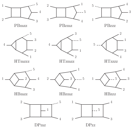
Figure 3: Ordered two-loop integral families entering the IBP reduction: three pentagon-boxes (PB), three hexagon-triangles (HT), three hexagon-boxes (HB), and two double-pentagons (DP).

	$A_{34}^{(2),N_{c}^{2}}$	$A_{34}^{(2),1}$	$A_{34}^{(2),1/N_{c}^{2}}$	$A_{\delta}^{(2),N_{c}}$	$A_{\delta}^{(2),1/N_{c}}$	NeatIBP file size
# of scalar integrals	20905	147235	83731	215394	204375
$N_{\mathrm{perm}}$(PBmzz)	2	16	7	8	8	8MB
$N_{\mathrm{perm}}$(PBzmz)	1	7	4	4	3	10MB
$N_{\mathrm{perm}}$(PBzzz)	2	4	7	12	24	5.9MB
$N_{\mathrm{perm}}$(HTmzzz)	2	8	12	24	24	1.9MB
$N_{\mathrm{perm}}$(HTzmzz)	2	14	8	24	20	3.8MB
$N_{\mathrm{perm}}$(HTzzzz)	1	4	4	12	12	4MB
$N_{\mathrm{perm}}$(HBmzz)	0	10	6	10	12	17MB
$N_{\mathrm{perm}}$(HBzmz)	0	5	3	5	5	13MB
$N_{\mathrm{perm}}$(HBzzz)	0	4	2	6	6	38MB
$N_{\mathrm{perm}}$(DPmz)	0	18	8	16	24	71MB
$N_{\mathrm{perm}}$(DPzz)	0	4	1	2	2	376MB

Table 1: Number of scalar integrals appearing in the two-loop $0\to\bar{b}bggH$ partial amplitudes at the various orders in $N_{c}$ without closed fermion loops. For each partial amplitude, we report the number of external leg permutations, $N_{\mathrm{perm}}$, for each of the ordered integral families shown in Figure 3, together with the file size of the corresponding IBP relations as produced by NeatIBP, which are stored in uncompressed text files as Mathematica expressions.

Next, the master integrals are expressed, order by order in $\epsilon$, as $\mathbb{Q}$-linear combinations of monomials of pentagon functions and transcendental constants ($\mathrm{i}\pi$ and $\zeta_{3}$) Chicherin:2021dyp ; Abreu:2023rco , denoted $m_{i}(f)$. The rational coefficients multiplying the master integrals are instead Laurent-expanded around $\epsilon=0$ within the finite-field workflow Peraro:2019svx . The $\epsilon$-expansion is truncated at $\mathcal{O}(\epsilon^{2})$ at one loop and $\mathcal{O}(\epsilon^{0})$ at two loops:

$$\sum_{\mathrm{pol}}T^{\dagger}_{\mathrm{gg}/\mathrm{q\bar{q}},i}A^{(L)}_{\mathrm{gg}/\mathrm{q\bar{q}}}=\sum_{p=-2L}^{-2L+4}\sum_{j}\epsilon^{p}\;e^{(L)}_{\mathrm{gg}/\mathrm{q\bar{q}};ij,p}(\vec{s})\;m_{j,p}(f)\;+\;\mathcal{O}(\epsilon^{-2L+5})\,,\quad L\in\{1,2\}.$$ (49)

We then convert the contracted amplitude to the helicity amplitude according to Eq. (46). Our setup allows for the simultaneous computation of multiple helicity configurations for a given partial sub-amplitude. In this view, we define the following sets of helicity amplitudes for $0\to\bar{b}bggH$ and $0\to\bar{b}b\bar{q}qH$,

$$A^{(L),\vec{h}_{g}}_{\mathrm{gg}} =\begin{pmatrix}A^{(L)}_{\mathrm{gg}}(1_{\bar{b}}^{+},2_{b}^{+},3_{g}^{+},4_{g}^{+},5_{H})\\ A^{(L)}_{\mathrm{gg}}(1_{\bar{b}}^{+},2_{b}^{+},3_{g}^{+},4_{g}^{-},5_{H})\\ A^{(L)}_{\mathrm{gg}}(1_{\bar{b}}^{+},2_{b}^{+},3_{g}^{-},4_{g}^{-},5_{H})\end{pmatrix}\,,$$ (50a)

$$A^{(L),\vec{h}^{\prime}_{g}}_{\mathrm{gg}} =\begin{pmatrix}A^{(L)}_{\mathrm{gg}}(1_{\bar{b}}^{+},2_{b}^{+},3_{g}^{+},4_{g}^{+},5_{H})\\ A^{(L)}_{\mathrm{gg}}(1_{\bar{b}}^{+},2_{b}^{+},3_{g}^{+},4_{g}^{-},5_{H})\\ A^{(L)}_{\mathrm{gg}}(1_{\bar{b}}^{-},2_{b}^{-},3_{g}^{+},4_{g}^{+},5_{H})\end{pmatrix}\,,$$ (50b)

$$A^{(L),\vec{h}_{q}}_{\mathrm{q\bar{q}}} =\begin{pmatrix}A^{(L)}_{\mathrm{q\bar{q}}}(1_{\bar{b}}^{+},2_{b}^{+},3_{\bar{q}}^{+},4_{q}^{-},5_{H})\end{pmatrix}\,,$$ (50c)

as well as the following helicity tensor matrices,

$$\mathcal{T}^{\vec{h}_{g}}_{\mathrm{gg}} =\begin{pmatrix}T^{++++}_{\mathrm{gg},1}&\cdots&T^{++++}_{\mathrm{gg},8}\\ T^{+++-}_{\mathrm{gg},1}&\cdots&T^{+++-}_{\mathrm{gg},8}\\ T^{++--}_{\mathrm{gg},1}&\cdots&T^{++--}_{\mathrm{gg},8}\end{pmatrix}\,,$$ (51a)

$$\mathcal{T}^{\vec{h}^{\prime}_{g}}_{\mathrm{gg}} =\begin{pmatrix}T^{++++}_{\mathrm{gg},1}&\cdots&T^{++++}_{\mathrm{gg},8}\\ T^{+++-}_{\mathrm{gg},1}&\cdots&T^{+++-}_{\mathrm{gg},8}\\ T^{--++}_{\mathrm{gg},1}&\cdots&T^{--++}_{\mathrm{gg},8}\end{pmatrix}\,,$$ (51b)

$$\mathcal{T}^{\vec{h}_{q}}_{\mathrm{q\bar{q}}} =\begin{pmatrix}T^{+++-}_{\mathrm{q\bar{q}},1}&\cdots&T^{+++-}_{\mathrm{q\bar{q}},8}\end{pmatrix}\,.$$ (51c)

For $0\to\bar{b}bggH$ we define a second set of helicity configurations ($\vec{h}^{\prime}_{g}$) in addition to the default one in Eq. (16) ($\vec{h}_{g}$) because the $A^{(2),1}_{34}$ and $A^{(2),1/N_{c}^{2}}_{34}$ sub-leading colour partial amplitudes are moderately easier to compute with $\vec{h}^{\prime}_{g}$ than with $\vec{h}_{g}$. We express the helicity tensor matrices $\mathcal{T}^{\vec{h}_{g}}_{\mathrm{gg}}$, $\mathcal{T}^{\vec{h}^{\prime}_{g}}_{\mathrm{gg}}$ and $\mathcal{T}^{\vec{h}_{q}}_{\mathrm{q\bar{q}}}$ in terms of the momentum-twistor variables $\vec{x}$ defined in Section 2.1.

The helicity amplitudes for a given set of helicity configurations $\vec{H}\in\{\vec{h}_{g},\vec{h}^{\prime}_{g},\vec{h}_{q}\}$ are then given by

$$A^{(L),\vec{H}}_{\mathrm{gg}/\mathrm{q\bar{q}};i} =\sum_{p=-2L}^{-2L+4}\,\sum_{jkl}\,\mathcal{T}^{\vec{H}}_{\mathrm{gg}/\mathrm{q\bar{q}},ij}(\vec{x})\,\left[\Theta^{-1}_{\mathrm{gg}/\mathrm{q\bar{q}}}(\vec{s})\right]_{jk}\,\epsilon^{p}\;e^{(L)}_{\mathrm{gg}/\mathrm{q\bar{q}};kl,p}(\vec{s})\;m_{l,p}(f)\;+\;\mathcal{O}(\epsilon^{-2L+5})\,,$$ (52)

$$=\sum_{p=-2L}^{-2L+4}\,\sum_{j}\,\epsilon^{p}\;g^{(L),\vec{H}}_{\mathrm{gg}/\mathrm{q\bar{q}};ij,p}(\vec{x})\;m_{j,p}(f)\;+\;\mathcal{O}(\epsilon^{-2L+5})\,,$$ (53)

for $L\in\{1,2\}$. All operations on rational functions from Eq. (47) to Eq. (53) are performed numerically using finite field arithmetic within FiniteFlow. Also the change of variables $\vec{s}\to\vec{x}$ required to go from Eq. (52) to Eq. (52) (given in Eq. (47)) is implemented within the finite-field framework.

At this stage, therefore, we have constructed a numerical algorithm to evaluate the rational coefficients of the pentagon-function monomials in the helicity amplitudes ($g^{(L),\vec{H}}_{\mathrm{gg}/\mathrm{q\bar{q}};ij,p}(\vec{x})$ in Eq. (53)) over finite fields. The remaining task is to perform the functional reconstruction of the rational coefficients from their numerical finite-field samples. This task is however made challenging by the high polynomial degrees, which leads to the need to evaluate a large number of sample points, as well as by the slow evaluation time, which is due to large number of integral family permutations in the IBP reduction step and to the complexity of the integrands. To alleviate this issue, we implement a number of optimisations to reduce the required number of sample points, following the strategy introduced in Refs. Badger:2021nhg ; Badger:2021imn .

	$A_{34}^{(2),N_{c}^{2}}$	$A_{34}^{(2),1}$		$A_{\delta}^{(2),N_{c}}$		$A_{\delta}^{(2),1/N_{c}}$
helicity set	$\vec{h}_{g}$	$\vec{h}^{\prime}_{g}$		$\vec{h}_{g}$		$\vec{h}_{g}$
$x_{1}=1$	133/132	176/175	176/175	265/269	265/269	214/207	214/207
ansatz for linear relations	-	-	$A_{34}^{(2),1/N_{c}^{2}}$	-	$A_{34}^{(2),1}$ $A_{43}^{(2),1}$ $A_{34}^{(2),1/N_{c}^{2}}$ $A_{43}^{(2),1/N_{c}^{2}}$ $A_{\delta}^{(2),1/N_{c}}$	-	$A_{34}^{(2),1}$ $A_{43}^{(2),1}$ $A_{34}^{(2),1/N_{c}^{2}}$ $A_{43}^{(2),1/N_{c}^{2}}$
linear relations	133/132	176/175	110/109	233/233	121/115	141/140	135/130
number of independent coefficients	162	572	216	582	151	581	258
denominator matching	133/0	176/0	110/0	233/0	119/0	141/0	135/0
univariate partial fraction	32/25	38/33	25/22	36/33	36/33	32/28	32/28
factor matching	28/0	38/0	24/0	36/0	36/0	32/0	32/0
number of sample points	16711	47608	10382	38221	37002	21150	20337
evaluation time per point	$t_{0}$	$100t_{0}$	$67t_{0}$	$106t_{0}$	$57t_{0}$	$74t_{0}$	$62t_{0}$

Table 2: Functional reconstruction data for the three most complicated two-loop subleading colour $0\to\bar{b}bggH$ amplitudes, as well as for the most complicated two-loop leading colour amplitude, for comparison. We report the maximal numerator/denominator polynomial degree of the rational coefficients appearing in the bare amplitude ($g^{(L),\vec{H}}_{\mathrm{gg};ij,p}$ in Eq. (53)) at each stage of the reconstruction strategy discussed in the text. We also show the number of independent rational coefficients, the number of sample points required to fully reconstruct the coefficients analytically, and the evaluation time for each finite-field point relative to that of the leading colour amplitude. The fourth row lists the partial sub-amplitudes used to construct the ansatz for the rational coefficients (see Eq. (54)), with - meaning that no ansatz is made.

The first, trivial, step of optimisation is to set $x_{1}=1$. Reinstating the $x_{1}$ dependence after the reconstruction is straightforward: $x_{1}$ is in fact the only dimensionful quantity in our momentum-twistor parametrisation, and therefore it appears only as a global prefactor of the amplitude. Additionally, as the pentagon-function monomials $m_{i}(f)$ contain also square roots, we introduce powers of $x_{1}$ in the monomials in order to keep them dimensionless. Secondly, we search for linear relations among the rational coefficients appearing in Eq. (53) numerically over finite fields, and only reconstruct the linearly independent ones, which are chosen so as to minimise the polynomial degrees. This procedure can be enhanced by including in the linear relations an ansatz for the rational coefficients. We construct this ansatz out the rational coefficients of the partial sub-amplitudes which have already been reconstructed. In practice, when reconstructing the list of coefficients $\{g^{(L),\vec{H}}_{\mathrm{gg}/\mathrm{q\bar{q}};ij,p}(\vec{x})\}$, we first determine the linear relations

$$\sum_{ijp}a_{ijp}\;g^{(L),\vec{H}}_{\mathrm{gg}/\mathrm{q\bar{q}};ij,p}(\vec{x})+\sum_{ijp}b_{ijp}\;\tilde{g}^{(L),\vec{H}}_{\mathrm{gg}/\mathrm{q\bar{q}};ij,p}(\vec{x})\;=\;0\,,$$ (54)

where $a_{ijp},b_{ijp}\in\mathbb{Q}$, and $\{\tilde{g}^{(L),\vec{H}}_{\mathrm{gg}/\mathrm{q\bar{q}};ij,p}(\vec{x})\}$ are the rational coefficients of partial sub-amplitudes which have already been computed. We then solve the relations in Eq. (54), preferring the known $\{\tilde{g}^{(L),\vec{H}}_{\mathrm{gg}/\mathrm{q\bar{q}};ij,p}(\vec{x})\}$ over the unknown $\{g^{(L),\vec{H}}_{\mathrm{gg}/\mathrm{q\bar{q}};ij,p}(\vec{x})\}$, and the simpler $\{g^{(L),\vec{H}}_{\mathrm{gg}/\mathrm{q\bar{q}};ij,p}(\vec{x})\}$ over the more complicated ones. Once we have an independent set of rational coefficients, we determine the analytic form of their denominators by matching them onto ansätze built out of the symbol letters Abreu:2023rco and a collection of simple spinor products on a univariate phase-space slice. Using this information and the polynomial degrees of the unknown numerators, we perform an on-the-fly univariate partial fraction decomposition with respect to $x_{5}$ of the independent rational coefficients. This is also achieved by writing an ansatz for the partial fraction decomposition, and reconstructing the coefficients in the ansatz, which are functions $(x_{2},x_{3},x_{4},x_{6})$. Finally, we perform another factor matching on a univariate slice, enlarging the ansatz so as to include also the spurious denominator factors introduced by the univariate partial fraction decomposition Badger:2021imn . The remaining numerators of the coefficients of the partial fraction decompositions are reconstructed using FiniteFlow’s built-in functional reconstruction algorithm Peraro:2016wsq .

In Table 2, we show the maximum polynomial degrees in the numerator and denominator of the rational coefficients of the pentagon-function monomials at each stage of the reconstruction strategy outlined above, for the three most complicated two-loop subleading colour $0\to\bar{b}bggH$ amplitudes, as well as for the most complicated two-loop leading colour amplitude, for comparison. The rest of the $0\to\bar{b}bggH$ amplitudes and all of the $0\to\bar{b}b\bar{q}qH$ amplitudes are rather straightforward to reconstruct, and hence we do not present their reconstruction data. We observe in Table 2 that, prior to performing any optimisation, the maximum polynomial degree of the rational coefficients in the sub-leading colour amplitudes is significantly higher than in the leading colour case. For $A_{\delta}^{(2),N_{c}}$ and $A_{\delta}^{(2),1/N_{c}}$, solving the linear relations without any ansatz leads to a drop in the maximum polynomial degree, while the latter stays the same for $A^{(2),1}_{34}$. Using an ansatz from other partial amplitudes decreases the maximum polynomial degrees quite significantly for all three subleading colour amplitudes. At the final optimisation stage, the numbers of required sample points are also smaller when the linear relations include coefficient ansätze, although the difference for $A_{\delta}^{(2),N_{c}}$ and $A_{\delta}^{(2),1/N_{c}}$ is not significant. The reduction in the number of sample points is however accompanied by a speed-up in the finite-field evaluation when the coefficient ansatz is included in the linear relations. To understand this, we recall that sampling the coefficients of the partial fraction decomposition involves the solution of a linear system of equations, which increases the evaluation time by a factor which is roughly equal to the number of terms in the ansätze for the partial fraction decomposition Badger:2021imn . From the last row of Table 2, we thus see that, although the coefficient ansatz does not reduce the maximum degrees for $A_{\delta}^{(2),N_{c}}$ and $A_{\delta}^{(2),1/N_{c}}$, it does make the finite-field sampling faster by shortening the partial fractioning ansätze. Finally, we see a slow-down of at least 50 times from the most complicated leading colour partial amplitude to the most complicated subleading colour one. This can be attributed to: (i) the larger number of integral family permutations appearing in the IBP reduction, (ii) the more complicated IBP systems that contribute, most notably DPmz and DPzz families, and (iii) the larger size of the integrands, as represented by the number of scalar Feynman integrals shown in Table 1. Additionally, the memory usage for the subleading colour amplitudes presented in Table 2 is roughly 3 times higher than for the most complicated leading colour amplitude.

With the functional reconstruction strategy discussed above we are finally able to obtain the analytic expression of the bare helicity amplitudes for the helicity configurations listed in Eq. (50). In order to present the $0\to\bar{b}bggH$ finite remainders for the independent helicity configurations in Eq. (16), we convert the $A^{(2),1;--++}_{34}$ and $A^{(2),1/N_{c}^{2};--++}_{34}$ bare amplitudes into $A^{(2),1;++--}_{34}$ and $A^{(2),1/N_{c}^{2};++--}_{34}$. We then extract the finite remainders from the bare amplitudes according to Eq. (27). The helicity-dependent finite remainders now take the form

$$F^{(L),h_{1}h_{2}h_{3}h_{4}}_{\mathrm{gg}/\mathrm{q\bar{q}}}=\sum_{p=0}^{-2L+4}\sum_{i}\,\epsilon^{p}\,r^{(L),h_{1}h_{2}h_{3}h_{4}}_{\mathrm{gg}/\mathrm{q\bar{q}};i,p}(\vec{x})\;m_{i,p}(f)\;+\;\mathcal{O}(\epsilon^{-2L+5})\,,\quad L\in\{1,2\}.$$ (55)

In order to optimise the expressions, we write all finite remainders for each loop order and helicity configuration in terms of a global set of linearly independent coefficients, chosen so as to minimise the polynomial degrees. We then perform a multivariate partial fraction decomposition of the independent coefficients by means of pfd-parallel Bendle:2021ueg . Following the strategy outlined in Ref. Badger:2024sqv , we decompose each addend in the univariate partial-fractioned representation rather than the complete coefficients. For the terms whose univariate partial-fractioned representation was more compact than the multivariate one, we kept the former. This approach does not remove the spurious factors introduced by the univariate partial fraction decomposition, but it is considerably faster and still makes the expressions more compact. Finally, we write the addends of the partial-fractioned coefficients in terms of independent irreducible factors, collected across each set of independent coefficients.

3.3 Validation

In this section we list the checks we have performed to validate our results.

• Comparison against direct helicity amplitude calculation

  We set up the direct computation of the helicity amplitudes as an alternative to the tensor-decomposition method discussed in Section 3.1. In this approach, the helicity-dependent loop numerators are constructed directly from the Feynman diagrams, and further expressed as linear combinations of scalar Feynman integrals. The subsequent steps are the same as described in Section 3.2. More details on the direct helicity amplitude approach can be found in Refs. Hartanto:2019uvl ; Badger:2021owl ; Badger:2021imn ; Badger:2021ega ; Badger:2023mgf ; Badger:2023xtl . We cross-checked the two approaches at the level of the bare amplitudes in the form of Eq. (53) for each independent helicity configuration by evaluating the rational coefficients at a non-physical, numerical phase-space point, while leaving pentagon functions, transcendental constants and square roots symbolic.

• Ward-identity test

  We check that the $0\to\bar{b}bggH$ amplitude vanishes upon replacing one of the gluon polarisation vectors with its momentum for each independent helicity configuration. In our test we replace $\varepsilon^{\mu}(p_{4})\rightarrow p_{4}$. In order to perform this test with the computational setup described in Section 3, we first modify the tensor decomposition in Eq. (37a) to

  $$A^{(L)}_{\mathrm{gg}}(\varepsilon(p_{4})\rightarrow p_{4}) =\sum_{i=1}^{4}\tilde{T}_{\mathrm{gg},i}\,\tilde{\omega}^{(L)}_{\mathrm{gg},i}\,,$$ (56)

  where

  $$\begin{aligned} \tilde{T}_{\mathrm{gg},1}&=\bar{u}(p_{2})v(p_{1})\;p_{1}\cdot\varepsilon(p_{3},q_{3})\,,\\ \tilde{T}_{\mathrm{gg},2}&=\bar{u}(p_{2})v(p_{1})\;p_{2}\cdot\varepsilon(p_{3},q_{3})\,,\\ \tilde{T}_{\mathrm{gg},3}&=\bar{u}(p_{2})\not{p}_{3}\not{p}_{4}v(p_{1})\;p_{1}\cdot\varepsilon(p_{3},q_{3})\,,\\ \tilde{T}_{\mathrm{gg},4}&=\bar{u}(p_{2})\not{p}_{3}\not{p}_{4}v(p_{1})\;p_{2}\cdot\varepsilon(p_{3},q_{3})\,.\end{aligned}$$ (57)

  As in Section. 3.1, we choose $q_{3}=p_{4}$ and use the gluon-polarisation vector sum specified in Eq. (42) for $\varepsilon(p_{3})$. The amplitude vanishes already upon contraction with the conjugated tensor structures given in Eq. (57), $\sum_{\mathrm{pol}}\tilde{T}^{\dagger}_{\mathrm{gg},i}A^{(L)}_{\mathrm{gg}}(\varepsilon(p_{4})\rightarrow p_{4})$, at the level of the master-integral representation in Eq (48). This check is done using a non-physical, numerical phase-space point for the master-integral coefficients while leaving the master integrals symbolic. The fact that the contracted amplitude vanishes in this Ward-identity check implies that the helicity amplitude vanishes as well. Additionally, we perform the Ward-identity check using the direct helicity amplitude setup, where the replacement $\varepsilon^{\mu}(p_{4})\rightarrow p_{4}$ is done directly in the construction of the helicity-dependent loop numerators.

• Pole cancellation

  The successful computation of the finite remainders following the prescription of Section 2.4 demonstrates that the $\epsilon$ poles are as expected from UV renormalisation and IR factorisation.

• $\mu$ dependence of the finite remainder

  We validate the $\mu$-restoring terms for the finite remainders given in Section 2.5 by evaluating numerically the finite remainders at two phase-space points, $\vec{s}_{A}$ and $\vec{s}_{B}$, related by an arbitrary rescaling factor $a$, as

  $$\vec{s}_{A} =\{s_{12},s_{23},s_{34},s_{45},s_{15},m_{H}^{2}\}\,,$$ (58a)

  $$\vec{s}_{B} =\frac{\vec{s}_{A}}{a}\,.$$ (58b)

  In terms of momentum-twistor variables, they correspond to

  $$\vec{x}_{A} =\{x_{1},x_{2},x_{3},x_{4},x_{5},x_{6}\}\,,$$ (59a)

  $$\vec{x}_{B} =\left\{\frac{x_{1}}{a},x_{2},x_{3},x_{4},x_{5},x_{6}\right\}\,.$$ (59b)

  We then verify that the following scaling relation holds,

  $$\frac{F^{(L)}(\vec{x}_{B},\mu=1)}{F^{(0)}(\vec{x}_{B})}=\frac{F^{(L)}(\vec{x}_{A},\mu=a)}{F^{(0)}(\vec{x}_{A})}\,,$$ (60)

  for all one- and two-loop helicity finite remainders.

• Comparison against OpenLoops at tree level and one loop

  We cross-checked the tree-level and one-loop hard functions against numerical results obtained from OpenLoops Buccioni:2019sur for both $0\to\bar{b}bggH$ and $0\to\bar{b}b\bar{q}qH$. We made use of OpenLoops’ pphbb process library and set $n_{f}=5$ to obtain the results in the 5FS.

4 Results

We obtained analytic expressions for the two-loop five-point amplitudes contributing to the double-virtual corrections to $b\bar{b}H$ production at the LHC, taking into account all colour contributions. The analytic form of the finite remainders and the corresponding $\epsilon$-pole terms (containing UV and IR singularities) up to two-loop level are provided in the ancillary files zenodo for the independent partial amplitudes and helicity configurations. We provide Mathematica scripts to evaluate numerically the bare amplitudes and the hard functions. In addition, the finite remainders and the evaluation of hard functions have been implemented in a C++ library which is also included in the ancillary files zenodo . We describe in detail the content of Mathematica ancillary files accompanying this paper in Appendix A. The content and usage instruction of the C++ library is described in the anc_cpp/README in the ancillary files zenodo . In this section, we present benchmark numerical evaluations of the hard functions for all channels relevant for the $pp\to b\bar{b}H$ scattering process, describe the implementation of the finite remainders in a C++ library and discuss certain analytic properties related to the pentagon functions.

4.1 Benchmark numerical evaluation of the hard functions

We evaluate the hard functions for all the partonic scattering channels contributing to $pp\to b\bar{b}H$:

$$gg\to\bar{b}bH :\qquad g(-p_{3})+g(-p_{4})\to\bar{b}(p_{1})+b(p_{2})+H(p_{5})\,,$$ (61a)

$$q\bar{q}\to\bar{b}bH :\qquad q(-p_{3})+\bar{q}(-p_{4})\to\bar{b}(p_{1})+b(p_{2})+H(p_{5})\,,$$ (61b)

$$\bar{q}q\to\bar{b}bH :\qquad\bar{q}(-p_{3})+q(-p_{4})\to\bar{b}(p_{1})+b(p_{2})+H(p_{5})\,,$$ (61c)

$$b\bar{b}\to\bar{b}bH :\qquad b(-p_{3})+\bar{b}(-p_{4})\to\bar{b}(p_{1})+b(p_{2})+H(p_{5})\,,$$ (61d)

$$\bar{b}b\to\bar{b}bH :\qquad\bar{b}(-p_{3})+b(-p_{4})\to\bar{b}(p_{1})+b(p_{2})+H(p_{5})\,,$$ (61e)

$$bb\to bbH :\qquad b(-p_{3})+b(-p_{4})\to b(p_{1})+b(p_{2})+H(p_{5})\,,$$ (61f)

$$\bar{b}\bar{b}\to\bar{b}\bar{b}H :\qquad\bar{b}(-p_{3})+\bar{b}(-p_{4})\to\bar{b}(p_{1})+\bar{b}(p_{2})+H(p_{5})\,.$$ (61g)

For this purpose, we need to apply permutations of the external momenta and/or parity conjugation to the independent partial finite remainders which we computed analytically in order to obtain the full set of partial finite remainders and helicity configurations. These operations are implemented differently on the pentagon functions and on their rational coefficients, as we describe below.

• For the rational coefficients of the pentagon-function monomials ($r^{(L),h_{1}h_{2}h_{3}h_{4}}_{\mathrm{gg}/\mathrm{q\bar{q}};j}(\vec{x})$ in Eq. (55)), the permutation of the external momenta is achieved by applying the permutation on the RHS of Eq. (9) before evaluating $\vec{s}$ and $\operatorname{\rm tr}_{\pm}$ numerically. This yields the values of the momentum-twistor variables at the permuted phase-space point. Similarly, in the case of parity conjugation, we exchange $\operatorname{\rm tr}_{+}\leftrightarrow\operatorname{\rm tr}_{-}$ on the RHS of Eq. (9). We stress that these operations can only be performed on momentum-twistor expressions which are free of spinor phases. The rational coefficients must therefore be divided by the appropriate spinor-phase factor, given in Eqs. (17) and (21), expressed in terms of momentum-twistor variables. The spinor-phase factor is then reinstated after applying the permutation and/or parity conjugation on its spinor expression — which retains the phase information — and converting it to momentum-twistor variables. We refer to Appendix C of Ref. Badger:2023mgf for a detailed discussion.

• The pentagon functions are evaluated numerically with the library PentagonFunctions++ PentagonFunctions:cpp . The evaluation for permutations of the external momenta can be obtained by expressing the permuted pentagon functions in terms of the unpermuted ones, so that the pentagon functions need to be evaluated only for the unpermuted external momenta. To derive such relations, the pentagon functions are first rewritten in terms of master-integral components, which are then permuted and expressed back in terms of unpermuted pentagon functions. The pentagon-function permutation rules are provided in the ancillary files. Note that the library PentagonFunctions++ requires the input phase-space point to be in a specific $2\to 3$ channel. The momenta used in this work ($p_{i}$) are related to the ones of Ref. Abreu:2023rco ($q_{i}$) by

  $$(q_{1},q_{2},q_{3},q_{4},q_{5})=(p_{5},p_{4},p_{3},p_{2},p_{1})\,,$$ (62)

  and we relabel the Mandelstam invariants of Ref. Abreu:2023rco by $t_{ij}=(q_{i}+q_{j})^{2}$, to distinguish them from ours ($s_{ij}$). Then, PentagonFunctions++ works in the $t_{45}$ channel, while the physical region relevant for our amplitudes is the $t_{23}$ ($s_{34}$) channel. In order to evaluate the pentagon functions in the $t_{23}$ channel, we evaluate them at a permuted phase-space point which belongs to the $t_{45}$ channel, $(q_{1},q_{4},q_{5},q_{2},q_{3})$, and apply the transformation which expresses the pentagon functions with $(q_{1},q_{2},q_{3},q_{4},q_{5})$ ordering in terms of those with $(q_{1},q_{4},q_{5},q_{2},q_{3})$.

$0\to\bar{b}bggH$	$\mathcal{H}^{(0)}$ [GeV-2]	$\mathcal{H}^{(1)}/\mathcal{H}^{(0)}$	$\mathcal{H}^{(2)}/\mathcal{H}^{(0)}$
$gg\to\bar{b}bH$	$5.9300960\cdot 10^{-9}$	-0.0074420656	0.083709468
$0\to\bar{b}b\bar{q}qH$	$\mathcal{H}^{(0)}$ [GeV-2]	$\mathcal{H}^{(1)}/\mathcal{H}^{(0)}$	$\mathcal{H}^{(2)}/\mathcal{H}^{(0)}$
$q\bar{q}\to\bar{b}bH$	$2.6534235\cdot 10^{-10}$	-0.39272804	0.10382080
$\bar{q}q\to\bar{b}bH$	$2.6534235\cdot 10^{-10}$	-0.049218183	0.10470723
$0\to\bar{b}b\bar{b}bH$	$\mathcal{H}^{(0)}$ [GeV-2]	$\mathcal{H}^{(1)}/\mathcal{H}^{(0)}$	$\mathcal{H}^{(2)}/\mathcal{H}^{(0)}$
$b\bar{b}\to\bar{b}bH$	$1.9980726\cdot 10^{-9}$	-0.0029434331	0.013659790
$\bar{b}b\to\bar{b}bH$	$2.2951653\cdot 10^{-8}$	0.26157437	0.046471305
$bb\to bbH$	$1.0166396\cdot 10^{-8}$	0.32618581	0.068890688
$\bar{b}\bar{b}\to\bar{b}\bar{b}H$	$1.0166396\cdot 10^{-8}$	0.32618581	0.068890688

Table 3: Numerical values of the hard functions defined in Eqs. (30) for the partonic scattering channels listed in Eqs. (61) using the phase-space point and input parameters given in Eqs. (63) and (64).

In Table 3, we show benchmark numerical values for the tree-level, one-loop and two-loop hard functions using a physical phase-space point associated with the $pp\to b\bar{b}H$ scattering process,

$$\begin{aligned} p_{1}&=(457.490386921,-279.844382235,-140.455057318,-333.552024023)\,,\\ p_{2}&=(403.008270188,228.438854552,143.939260340,299.186973151)\,,\\ p_{3}&=(-500,0,0,-500)\,,\\ p_{4}&=(-500,0,0,500)\,,\\ p_{5}&=(139.501342891,51.4055276828,-3.48420302179,34.3650508716)\,,\end{aligned}$$ (63)

with the following values of the input parameters:

$$\mu=173.2\,,\qquad\alpha_{s}=0.118\,,\qquad y_{b}=0.0192916457706\,.$$ (64)

The momenta $p_{i}$ and the renormalisation scale $\mu$ are given in the units of GeV. Benchmark numerical results for the bare helicity amplitudes separately for all partial amplitudes and ($N_{c}$, $n_{f}$) contributions are provided in the ancillary files.

4.2 Numerical implementation

We implemented all finite remainders in a C++ library to yield the IR and UV finite squared matrix elements after colour and helicity sums as needed for differential cross sections. To this end, we employ the PentagonFunctions++ Chicherin:2020oor library and the qd library QDlib whenever higher numerical precision is needed. The implementation has been cross-checked against the independent Mathematica implementation used to derive the benchmark values in Table 3, for a couple of phase-space points. To ensure the numerical stability of the matrix elements for a given phase space point $p$ and renormalisation scale $\mu$, we employ the following rescue strategy (similar to Ref. Badger:2023mgf ) to successively increase the numerical precision if needed:

1. The matrix element is evaluated in standard double precision for the rational and transcendental (i.e., the pentagon functions) parts at the given phase-space point as well as in a rescaled point $p^{\prime}=\{a\times p_{i}\}_{i=1}^{5}$, $\mu^{\prime}=a\times\mu$. Here $a$ is a numerical constant (in practice, we use $a=10$).

2. We exploit the scaling properties of the matrix element to compute the relative difference between those two points

   $$r^{\text{diff}}=\frac{|\mathcal{H}^{(2)}(p,\mu)-a^{2}\,\mathcal{H}^{(2)}(p^{\prime},\mu^{\prime})|}{|\mathcal{H}^{(2)}(p,\mu)+a^{2}\,\mathcal{H}^{(2)}(p^{\prime},\mu^{\prime})|}\;.$$ (65)

   From this quantity, we define the estimate of the number of correct digits as

   $$n^{\text{cor}}=-\log_{10}(r^{\text{diff}})\;.$$ (66)

3. We demand at least four digits, i.e., $n^{\text{cor}}>4$, for a phase space point to be accepted. If the estimated precision is insufficient, we restart from 1) with a higher numerical precision.

We implement the following four precision levels:

• sd/sd: the rational and transcendental parts are evaluated in standard double-precision.

• dd/sd: the rational part is evaluated at double-double precision ($\approx 32$ digits) while the transcendental part is kept at double precision.

• qd/sd: same as before but with quad-double precision ($\approx 64$ digits).

• qd/dd: same as previous but with the transcendental part in double-double precision.

To test the stability in a realistic example, we define a simple $b\bar{b}H$ phase space by requiring two anti-$k_{T}$ ($R=0.4$) $b$ jets with a transverse momentum of at least $25$ GeV and an absolute rapidity of at most $2.5$. We generate random points in this phase space and evaluate the two-loop finite remainders while keeping track of the number of correct digits achieved. In Figure 4, we present the resulting distribution of correct digits organised in two sets of initial state channels $q\bar{q}/b\bar{b}/bb/\bar{b}\bar{b}$ and $gg$. Most of the points reach the stability goal with double-precision arithmetic. In the case of four-quark amplitudes, only $2-3$ permille of the points require a re-evaluation in higher precision arithmetic. These points appear to suffer mainly from the numerical accuracy of the transcendental part, as higher precision evaluation of the rational part does not improve the number of accurate digits. One permille of the points must be evaluated using double-double precision for the pentagon functions. For the two-quark two-gluon amplitudes, about 8 percent do not reach the accuracy goal with double-precision arithmetic. However, most unstable points can be rescued using higher precision rationals and, similarly to the quark-only amplitudes, only about one permille requires higher precision for the transcendental parts.

We find an average evaluation time of about 40 seconds for the amplitudes on a Intel(R) Xeon(R) Silver 4116 CPU @ 2.10GHz CPU. The time estimate contains the re-evaluation with the rescaled points to assess the numerical stability and potential higher-precision evaluations. These times are sufficiently short to ensure that the evaluation of the two-loop contribution to the physical cross sections is not the bottleneck of a next-to-next-to-leading order computation.

In addition to the stability analysis we computed the double virtual contribution to the total cross section for the above phase space and estimate it to be approximately 10% with respect to the leading-order cross-section. Furthermore, we computed the contribution in the leading-colour approximation and estimate the effect of sub-leading colour terms to be about $\approx 2\%$ with respect to leading-order.

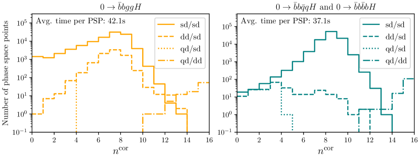
Figure 4: Estimated numerical precision of $\mathcal{H}^{(2)}(p,\mu)$ evaluated for phase-space points arising during Monte Carlo integration given in terms of number of estimated correct digits. The results are separated according to the channels ($q\bar{q}/b\bar{b}/bb/\bar{b}\bar{b}$ and $gg$). Only points that fail the $n^{\text{cor}}>4$ requirement are re-evaluated at the next higher numerical precision implemented. The estimated evaluation times contain the re-evaluations and are also averaged over the higher precision evaluations, and therefore represent the realistic times per phase-space point during Monte Carlo integration. In total 100000 points have been evaluated for each channel.

4.3 Analytic properties

We confirm the observations made in Ref. Badger:2024sqv regarding the analytic structure of the amplitudes, and refer to Section 4.2 thereof for a detailed discussion. Here we content ourselves with recalling the most important features. In particular, we observe that the symbol letter $\sqrt{\Delta_{5}}$ drops out of the finite remainders, while the six letters $\sqrt{\Sigma_{5}^{(i)}}$ ($i=1,\ldots,6$) are absent already from the bare amplitudes (see Ref. Abreu:2023rco for the definition of $\Delta_{5}$ and $\Sigma_{5}^{(i)}$, which are degree-4 polynomials in the Mandelstam invariants $\vec{s}$). Thanks to the criteria adopted in the definition of the pentagon functions Chicherin:2021dyp ; Abreu:2023rco , these letters are by construction isolated into minimal subsets of pentagon functions, and their cancellation is thus made manifest by the cancellation of the corresponding sets of pentagon functions. This makes the analytic structure of the expressions more transparent, and the numerical evaluation more efficient. We stress in particular that all pentagon functions which diverge in the physical phase space are absent, whereas all pentagon functions that do not involve the letters $\sqrt{\Delta_{5}}$ and $\sqrt{\Sigma_{5}^{(i)}}$ are present.

5 Conclusion

In this work we have presented the two-loop five-particle amplitudes contributing to $pp\to b\bar{b}H$ production at the LHC in the five-flavour scheme where the bottom-quark is treated as a massless particle and the bottom-Yukawa coupling is kept finite. We derived analytic expressions of the finite remainders up to two-loop level in perturbative QCD, taking into account the complete colour structure. This is the first time analytic results are derived for a full colour two-loop five-point amplitude with an external mass.

The finite remainders are written in terms of one-mass pentagon functions and rational coefficients, which we reconstructed from multiple numerical evaluations over finite fields. Our finite-field framework combines the Feynman diagram, four-dimensional projector and integral reduction methods, with optimised IBP relations obtained by means of NeatIBP. We employed a number optimisations to reduce the complexity of the functional reconstruction of the rational coefficients, such as finding linear relations among them and ansätze, guessing the denominators using letters of the alphabet, and performing on-the-fly univariate partial fraction decomposition. We observe that the analytic reconstruction of the subleading colour amplitudes requires a significantly larger number of sample points than in the leading colour case, and that the memory usage and evaluation time per point per finite field are also substantially higher. We alleviated this by exploiting linear relations among the rational coefficients across various subleading colour contributions. We simplified the resulting analytic expressions of the rational coefficients through multivariate partial fraction decomposition with pfd-parallel.

We confirm the observations made in Ref. Badger:2024sqv regarding the analytic structure of the amplitudes: the non-planar letters $\sqrt{\Sigma_{5}^{(i)}}$ ($i=1,\ldots,6$) and the non-planar pentagon functions which diverge in the physical region are absent from the bare amplitudes, while the letter $\sqrt{\Delta}_{5}$ drops out of the finite remainders. These non-trivial cancellations call for a theoretical explanation.

We implemented all finite remainders in a C++ library and assess the numerical stability of the evaluation of the hard functions. We find that the stability and evaluation time are suitable for immediate deployment in the computation of differential distributions at NNLO QCD accuracy. The numerical implementation is provided as a C++ package.

Our results, together with the implementation of the pentagon functions in the PentagonFunctions++ library, open the door to an efficient computation of the double-virtual corrections to $pp\to H+2b$ jets at NNLO QCD accuracy in the 5FS, as well as in an approximated 4FS where the leading $m_{b}$ contributions are included through massification. In addition, also by employing massification procedure, our full-colour two-loop $pp\to b\bar{b}H$ amplitudes can be used to approximate full-colour two-loop $pp\to t\bar{t}H$ amplitudes in the high-energy region Devoto:2024nhl .

Appendix A Description of the ancillary files

In this Appendix, we describe the content of the Mathematica ancillary files, which can be downloaded from zenodo . The description of the C++ library, on the other hand, can be found in the anc_cpp/README in the ancillary files zenodo . The analytic expressions are given separately for the finite remainders and the $\epsilon$-pole terms that contain the UV and IR singularities. The $L$-loop finite remainders $F^{(L)}$ are presented in the form

$$F^{(L)}=\sum_{p=0}^{-2L+4}\epsilon^{p}\,\sum_{ij}r_{i}(\vec{y})\,S_{pij}\,m_{j}(f)\,,\qquad L\in\{1,2\}\,,$$ (67)

where $r_{i}$ is a set of independent rational coefficients collected across finite remainders with the same helicity configuration and loop order, $S$ is a sparse matrix of rational numbers, and $m_{j}(f)$ are monomials built up of pentagon functions, transcendental constants, square roots, and power of $x_{1}$. The latter are included in the monomials to keep them dimensionless. The rational coefficients, $r_{i}(\vec{y})$ in Eq. (67), are expressed in terms of distinct polynomial factors $y_{i}(\vec{x})$, common for each set of $r_{i}$’s. We recall that the analytic expressions are derived with $x_{1}=1$. While the $x_{1}$ dependence in the monomials $m_{j}(f)$ is explicitly reinstated in the provided expressions, that of the rational coefficients is recovered in the numerical evaluation scripts.

All analytical results derived in this paper are distributed in Mathematica-readable format. In the following we give the translations of the symbols used in the ancillary files to the notation used in the paper.

• Partonic scattering processes contributing to $pp\to b\bar{b}H$:

  $$\begin{aligned} \texttt{2g2bH}&=0\to\bar{b}bggH\,,\\ \texttt{2q2bH}&=0\to\bar{b}b\bar{q}qH\,.\end{aligned}$$ (68)

• Colour factors in $0\to\bar{b}bggH$:

  $$\begin{aligned} \texttt{T2341}&=(t^{a_{3}}t^{a_{4}})_{i_{2}}^{\;\;\bar{i}_{1}}\,,\\ \texttt{d12d34}&=\delta_{i_{2}}^{\;\;\bar{i}_{1}}\delta^{a_{3}a_{4}}\,.\end{aligned}$$ (69)

• Colour factors in $0\to\bar{b}b\bar{q}qH$:

  $$\begin{aligned} \texttt{d14d23}&=\delta_{i_{4}}^{\;\;\bar{i}_{1}}\delta_{i_{2}}^{\;\;\bar{i}_{3}}\,,\\ \texttt{d12d34}&=\delta_{i_{2}}^{\;\;\bar{i}_{1}}\delta_{i_{4}}^{\;\;\bar{i}_{3}}\,.\end{aligned}$$ (70)

• Helicity configurations:

  $$\begin{aligned} \texttt{pppp}&=++++\,,\\ \texttt{pppm}&=+++-\,,\\ \texttt{ppmm}&=++--\,.\end{aligned}$$ (71)

• Dimensional regulator, momentum-twistor variables, Mandelstam invariants and other kinematical quantities needed to evaluate the amplitude:

  $$\begin{aligned} \texttt{eps}&=\epsilon\,,\\ \texttt{ex[i]}&=x_{i}\quad\forall i=1,\dots,6\,,\\ \texttt{s[i,j]}\;\mathrm{or}\;\texttt{sij}&=s_{ij}\,,\\ \texttt{s[i,j,k]}\;\mathrm{or}\;\texttt{sijk}&=s_{ijk}\,,\\ \texttt{tr5}&=\operatorname{\rm tr}_{5}\,,\\ \texttt{trp[i,j,k,l]}&=\operatorname{\rm tr}_{+}(ijkl)\,,\\ \texttt{trm[i,j,k,l]}&=\operatorname{\rm tr}_{-}(ijkl)\,.\\ \end{aligned}$$ (72)

• Pentagon functions (F[w,i]), transcendental constants and square roots (see Refs. Abreu:2023rco ; Chicherin:2021dyp for a more detailed description of these objects):

  $$\begin{aligned} \texttt{re[3,1]}&=\zeta_{3}\,,\\ \texttt{im[1,1]}&=\mathrm{i}\pi\,,\\ \texttt{sqrtDelta5}&=\sqrt{\Delta_{5}}\,,\\ \texttt{sqrtG3[i]}&=\sqrt{\Delta_{3}^{(i)}}\,,\\ \texttt{sqrtSigma5[i]}&=\sqrt{\Sigma_{5}^{(i)}}\,.\end{aligned}$$ (73)

• Renormalisation scale:

  $$\begin{aligned} \texttt{mu}&=\mu\,.\\ \end{aligned}$$ (74)

The content of the ancillary files is organised according to:

• scattering channel <proc> (2g2bH, 2q2bH),

• loop order <loop> (1, 2),

• colour factor <col>: (T2341 and d12d34 for $0\to\bar{b}bggH$, d14d23 and d12d34 for $0\to\bar{b}b\bar{q}qH$),

• powers of $n_{f}$ (<a>) and $N_{c}$ (<b>),

• helicity configuration <hel>: (pppp, pppm, ppmm).

We here list and describe all files we provided.

• amplitudes_<proc>/Tree_<proc>_<col>_Nfp<a>_Ncp<b>_<hel>.m: tree-level helicity amplitude.

• amplitudes_<proc>/FiniteRemainder_indep_coeffs_y_<loop>L_<proc>_<hel>.m: independent rational coefficients $r_{i}$ in Eq. (67) as functions of common factors y[i] ($y_{i}$).

• amplitudes_<proc>/FiniteRemainder_sm_<loop>L_<proc>_<col>_Nfp<a>_Ncp<b>_<hel>.m: rational matrix $S$ in Eq. (67), written in Mathematica’s SparseArray format.

• amplitudes_<proc>/ys_<loop>L_<proc>_<hel>.m: replacement rules for the common polynomial factors y[i] ($y_{i}$) in terms of momentum-twistor variables ex[i] ($x_{i}$).

• amplitudes_<proc>/FunctionBasis_<proc>_<loop>L.m: monomial basis of pentagon functions, transcendental constants and square roots ($m_{j}(f)$ in Eq. (67)).

• amplitudes_<proc>/mudep_<loop>L_<proc>_<col>_Nfp<a>_Ncp<b>_<hel>.m: $\mu$-restoring term derived from Eqs. (35) and (36).

• amplitudes_<proc>/Poles_<loop>L_<proc>_<col>_Nfp<a>_Ncp<b>_<hel>.m: pole terms built out of UV and IR counterterms, which take the same form as the bare helicity amplitude in Eq. (49) except that the rational coefficients are given separately for each helicity configuration. The pole terms are given in the following format,

  {coefficientrules,{coefficients,monomials}}  ,

  where coefficientrules is a list of replacement rules defining the independent rational coefficients f[i] in terms of the momentum-twistor variables ex[i], monomials and coefficients are the lists of pentagon-function monomials and of their coefficients, which depend on both eps ($\epsilon$) and the independent rational coefficients f[i].

• F_permutations_sm/: a folder containing the pentagon functions’ permutation rules. The permutation to the ordering <perm> of the external momenta is given by the matrix stored in sm_F_perm_2l5p1m_<perm>.m (in Mathematica’s SparseArray format). Multiplying the latter by the array of pentagon-function monomials in F_monomials.m gives the permutation of the pentagon functions listed in the variable listOfFunctions in utilities.m.

• Evaluate_BareAmplitudes_<proc>.wl: script to evaluate numerically the bare helicity partial amplitudes in the independent helicity configurations for the $gg\to\bar{b}bH$ and $\bar{q}q\to\bar{b}bH$ scattering channels as defined in Eq. (61).

• Evaluate_HardFunctions_<proc>.wl: script to evaluate numerically the hard functions for all partonic channels contributing to $pp\to b\bar{b}H$ as listed in Eq (61).

• utilities.m: a collection of auxiliary functions needed for the numerical evaluation scripts.

• IR_pole_operators/Z<loop>_<proc>.m: $\mathbf{Z}$ operator entering the IR-subtraction term, see Eqs. (27) and (29).

• IR_pole_operators/usage.wl: a script to construct the IR-subtraction terms from $\mathbf{Z}$.

References

- (1) ATLAS collaboration, G. Aad et al., Observation of a new particle in the search for the Standard Model Higgs boson with the ATLAS detector at the LHC, Phys. Lett. B 716 (2012) 1–29, [1207.7214].
- (2) CMS collaboration, S. Chatrchyan et al., Observation of a New Boson at a Mass of 125 GeV with the CMS Experiment at the LHC, Phys. Lett. B 716 (2012) 30–61, [1207.7235].
- (3) ATLAS collaboration, G. Aad et al., A detailed map of Higgs boson interactions by the ATLAS experiment ten years after the discovery, Nature 607 (2022) 52–59, [2207.00092].
- (4) CMS collaboration, A. Tumasyan et al., A portrait of the Higgs boson by the CMS experiment ten years after the discovery., Nature 607 (2022) 60–68, [2207.00043].
- (5) M. Cepeda et al., Report from Working Group 2: Higgs Physics at the HL-LHC and HE-LHC, CERN Yellow Rep. Monogr. 7 (2019) 221–584, [1902.00134].
- (6) LHC Higgs Cross Section Working Group collaboration, D. de Florian et al., Handbook of LHC Higgs Cross Sections: 4. Deciphering the Nature of the Higgs Sector, 1610.07922.
- (7) D. Pagani, H.-S. Shao and M. Zaro, RIP : how other Higgs production modes conspire to kill a rare signal at the LHC, JHEP 11 (2020) 036, [2005.10277].
- (8) C. Grojean, A. Paul and Z. Qian, Resurrecting with kinematic shapes, JHEP 04 (2021) 139, [2011.13945].
- (9) P. Konar, B. Mukhopadhyaya, R. Rahaman and R. K. Singh, Probing non-standard interaction at the LHC at TeV, Phys. Lett. B 818 (2021) 136358, [2101.10683].
- (10) C. Balazs, J. L. Diaz-Cruz, H. J. He, T. M. P. Tait and C. P. Yuan, Probing Higgs bosons with large bottom Yukawa coupling at hadron colliders, Phys. Rev. D 59 (1999) 055016, [hep-ph/9807349].
- (11) S. Dawson, C. B. Jackson, L. Reina and D. Wackeroth, Higgs production in association with bottom quarks at hadron colliders, Mod. Phys. Lett. A 21 (2006) 89–110, [hep-ph/0508293].
- (12) S. Manzoni, E. Mazzeo, J. Mazzitelli, M. Wiesemann and M. Zaro, Taming a leading theoretical uncertainty in HH measurements via accurate simulations for production, JHEP 09 (2023) 179, [2307.09992].
- (13) CMS collaboration, Search for the SM Higgs boson produced in association with bottom quarks in final states with leptons, .
- (14) D. Dicus, T. Stelzer, Z. Sullivan and S. Willenbrock, Higgs boson production in association with bottom quarks at next-to-leading order, Phys. Rev. D 59 (1999) 094016, [hep-ph/9811492].
- (15) C. Balazs, H.-J. He and C. P. Yuan, QCD corrections to scalar production via heavy quark fusion at hadron colliders, Phys. Rev. D 60 (1999) 114001, [hep-ph/9812263].
- (16) F. Maltoni, Z. Sullivan and S. Willenbrock, Higgs-Boson Production via Bottom-Quark Fusion, Phys. Rev. D 67 (2003) 093005, [hep-ph/0301033].
- (17) R. V. Harlander and W. B. Kilgore, Higgs boson production in bottom quark fusion at next-to-next-to leading order, Phys. Rev. D 68 (2003) 013001, [hep-ph/0304035].
- (18) A. Belyaev, P. M. Nadolsky and C. P. Yuan, Transverse momentum resummation for Higgs boson produced via b anti-b fusion at hadron colliders, JHEP 04 (2006) 004, [hep-ph/0509100].
- (19) R. V. Harlander, K. J. Ozeren and M. Wiesemann, Higgs plus jet production in bottom quark annihilation at next-to-leading order, Phys. Lett. B 693 (2010) 269–273, [1007.5411].
- (20) K. J. Ozeren, Analytic Results for Higgs Production in Bottom Fusion, JHEP 11 (2010) 084, [1010.2977].
- (21) S. Bühler, F. Herzog, A. Lazopoulos and R. Müller, The fully differential hadronic production of a Higgs boson via bottom quark fusion at NNLO, JHEP 07 (2012) 115, [1204.4415].
- (22) R. V. Harlander, S. Liebler and H. Mantler, SusHi: A program for the calculation of Higgs production in gluon fusion and bottom-quark annihilation in the Standard Model and the MSSM, Comput. Phys. Commun. 184 (2013) 1605–1617, [1212.3249].
- (23) R. V. Harlander, A. Tripathi and M. Wiesemann, Higgs production in bottom quark annihilation: Transverse momentum distribution at NNLONNLL, Phys. Rev. D 90 (2014) 015017, [1403.7196].
- (24) T. Ahmed, M. Mahakhud, P. Mathews, N. Rana and V. Ravindran, Two-loop QCD corrections to Higgs amplitude, JHEP 08 (2014) 075, [1405.2324].
- (25) T. Gehrmann and D. Kara, The form factor to three loops in QCD, JHEP 09 (2014) 174, [1407.8114].
- (26) A. A H, P. Banerjee, A. Chakraborty, P. K. Dhani, P. Mukherjee, N. Rana et al., NNLO QCDQED corrections to Higgs production in bottom quark annihilation, Phys. Rev. D 100 (2019) 114016, [1906.09028].
- (27) C. Duhr, F. Dulat and B. Mistlberger, Higgs Boson Production in Bottom-Quark Fusion to Third Order in the Strong Coupling, Phys. Rev. Lett. 125 (2020) 051804, [1904.09990].
- (28) R. Mondini and C. Williams, Bottom-induced contributions to Higgs plus jet at next-to-next-to-leading order, JHEP 05 (2021) 045, [2102.05487].
- (29) C. Biello, A. Sankar, M. Wiesemann and G. Zanderighi, NNLO+PS predictions for Higgs production through bottom-quark annihilation with MINNLO, Eur. Phys. J. C 84 (2024) 479, [2402.04025].
- (30) J. M. Campbell, R. K. Ellis, F. Maltoni and S. Willenbrock, Higgs-Boson Production in Association with a Single Bottom Quark, Phys. Rev. D 67 (2003) 095002, [hep-ph/0204093].
- (31) S. Dawson and P. Jaiswal, Weak Corrections to Associated Higgs-Bottom Quark Production, Phys. Rev. D 81 (2010) 073008, [1002.2672].
- (32) S. Dawson, C. B. Jackson and P. Jaiswal, SUSY QCD Corrections to Higgs-b Production : Is the Approximation Accurate?, Phys. Rev. D 83 (2011) 115007, [1104.1631].
- (33) S. Dittmaier, M. Krämer and M. Spira, Higgs radiation off bottom quarks at the Tevatron and the CERN LHC, Phys. Rev. D 70 (2004) 074010, [hep-ph/0309204].
- (34) S. Dawson, C. B. Jackson, L. Reina and D. Wackeroth, Exclusive Higgs boson production with bottom quarks at hadron colliders, Phys. Rev. D 69 (2004) 074027, [hep-ph/0311067].
- (35) S. Dawson, C. B. Jackson, L. Reina and D. Wackeroth, Higgs boson production with one bottom quark jet at hadron colliders, Phys. Rev. Lett. 94 (2005) 031802, [hep-ph/0408077].
- (36) N. Liu, L. Wu, P. Wu and J. M. Yang, Complete one-loop effects of SUSY QCD in production at the LHC under current experimental constraints, JHEP 01 (2013) 161, [1208.3413].
- (37) S. Dittmaier, P. Häfliger, M. Krämer, M. Spira and M. Walser, Neutral MSSM Higgs-boson production with heavy quarks: NLO supersymmetric QCD corrections, Phys. Rev. D 90 (2014) 035010, [1406.5307].
- (38) N. Deutschmann, F. Maltoni, M. Wiesemann and M. Zaro, Top-Yukawa contributions to bbH production at the LHC, JHEP 07 (2019) 054, [1808.01660].
- (39) M. Wiesemann, R. Frederix, S. Frixione, V. Hirschi, F. Maltoni and P. Torrielli, Higgs production in association with bottom quarks, JHEP 02 (2015) 132, [1409.5301].
- (40) B. Jager, L. Reina and D. Wackeroth, Higgs boson production in association with b jets in the POWHEG BOX, Phys. Rev. D 93 (2016) 014030, [1509.05843].
- (41) L. Buonocore, S. Devoto, S. Kallweit, J. Mazzitelli, L. Rottoli and C. Savoini, Associated production of a W boson and massive bottom quarks at next-to-next-to-leading order in QCD, Phys. Rev. D 107 (2023) 074032, [2212.04954].
- (42) J. Mazzitelli, V. Sotnikov and M. Wiesemann, Next-to-next-to-leading order event generation for Z-boson production in association with a bottom-quark pair, 2404.08598.
- (43) S. Badger, H. B. Hartanto, J. Kryś and S. Zoia, Two-loop leading-colour QCD helicity amplitudes for Higgs boson production in association with a bottom-quark pair at the LHC, JHEP 11 (2021) 012, [2107.14733].
- (44) T. Gehrmann, J. M. Henn and N. A. Lo Presti, Analytic form of the two-loop planar five-gluon all-plus-helicity amplitude in QCD, Phys. Rev. Lett. 116 (2016) 062001, [1511.05409].
- (45) C. G. Papadopoulos, D. Tommasini and C. Wever, The Pentabox Master Integrals with the Simplified Differential Equations approach, JHEP 04 (2016) 078, [1511.09404].
- (46) S. Abreu, B. Page and M. Zeng, Differential equations from unitarity cuts: nonplanar hexa-box integrals, JHEP 01 (2019) 006, [1807.11522].
- (47) D. Chicherin, T. Gehrmann, J. M. Henn, N. A. Lo Presti, V. Mitev and P. Wasser, Analytic result for the nonplanar hexa-box integrals, JHEP 03 (2019) 042, [1809.06240].
- (48) D. Chicherin, T. Gehrmann, J. M. Henn, P. Wasser, Y. Zhang and S. Zoia, All Master Integrals for Three-Jet Production at Next-to-Next-to-Leading Order, Phys. Rev. Lett. 123 (2019) 041603, [1812.11160].
- (49) S. Abreu, L. J. Dixon, E. Herrmann, B. Page and M. Zeng, The two-loop five-point amplitude in super-Yang-Mills theory, Phys. Rev. Lett. 122 (2019) 121603, [1812.08941].
- (50) S. Abreu, H. Ita, F. Moriello, B. Page, W. Tschernow and M. Zeng, Two-Loop Integrals for Planar Five-Point One-Mass Processes, JHEP 11 (2020) 117, [2005.04195].
- (51) D. D. Canko, C. G. Papadopoulos and N. Syrrakos, Analytic representation of all planar two-loop five-point Master Integrals with one off-shell leg, JHEP 01 (2021) 199, [2009.13917].
- (52) S. Abreu, H. Ita, B. Page and W. Tschernow, Two-loop hexa-box integrals for non-planar five-point one-mass processes, JHEP 03 (2022) 182, [2107.14180].
- (53) A. Kardos, C. G. Papadopoulos, A. V. Smirnov, N. Syrrakos and C. Wever, Two-loop non-planar hexa-box integrals with one massive leg, JHEP 05 (2022) 033, [2201.07509].
- (54) S. Abreu, D. Chicherin, H. Ita, B. Page, V. Sotnikov, W. Tschernow et al., All Two-Loop Feynman Integrals for Five-Point One-Mass Scattering, Phys. Rev. Lett. 132 (2024) 141601, [2306.15431].
- (55) T. Gehrmann, J. M. Henn and N. A. Lo Presti, Pentagon functions for massless planar scattering amplitudes, JHEP 10 (2018) 103, [1807.09812].
- (56) D. Chicherin and V. Sotnikov, Pentagon Functions for Scattering of Five Massless Particles, JHEP 20 (2020) 167, [2009.07803].
- (57) D. Chicherin, V. Sotnikov and S. Zoia, Pentagon functions for one-mass planar scattering amplitudes, JHEP 01 (2022) 096, [2110.10111].
- (58) A. von Manteuffel and R. M. Schabinger, A novel approach to integration by parts reduction, Phys. Lett. B 744 (2015) 101–104, [1406.4513].
- (59) T. Peraro, Scattering amplitudes over finite fields and multivariate functional reconstruction, JHEP 12 (2016) 030, [1608.01902].
- (60) J. Klappert and F. Lange, Reconstructing rational functions with FireFly, Comput. Phys. Commun. 247 (2020) 106951, [1904.00009].
- (61) T. Peraro, FiniteFlow: multivariate functional reconstruction using finite fields and dataflow graphs, JHEP 07 (2019) 031, [1905.08019].
- (62) J. Klappert, S. Y. Klein and F. Lange, Interpolation of dense and sparse rational functions and other improvements in FireFly, Comput. Phys. Commun. 264 (2021) 107968, [2004.01463].
- (63) J. Klappert, F. Lange, P. Maierhöfer and J. Usovitsch, Integral reduction with Kira 2.0 and finite field methods, Comput. Phys. Commun. 266 (2021) 108024, [2008.06494].
- (64) J. Gluza, K. Kajda and D. A. Kosower, Towards a Basis for Planar Two-Loop Integrals, Phys. Rev. D 83 (2011) 045012, [1009.0472].
- (65) R. M. Schabinger, A New Algorithm For The Generation Of Unitarity-Compatible Integration By Parts Relations, JHEP 01 (2012) 077, [1111.4220].
- (66) H. Ita, Two-loop Integrand Decomposition into Master Integrals and Surface Terms, Phys. Rev. D 94 (2016) 116015, [1510.05626].
- (67) G. Chen, J. Liu, R. Xie, H. Zhang and Y. Zhou, Syzygies Probing Scattering Amplitudes, JHEP 09 (2016) 075, [1511.01058].
- (68) J. Böhm, A. Georgoudis, K. J. Larsen, M. Schulze and Y. Zhang, Complete sets of logarithmic vector fields for integration-by-parts identities of Feynman integrals, Phys. Rev. D 98 (2018) 025023, [1712.09737].
- (69) J. Bosma, K. J. Larsen and Y. Zhang, Differential equations for loop integrals without squared propagators, PoS LL2018 (2018) 064, [1807.01560].
- (70) J. Boehm, D. Bendle, W. Decker, A. Georgoudis, F.-J. Pfreundt, M. Rahn et al., Module Intersection for the Integration-by-Parts Reduction of Multi-Loop Feynman Integrals, PoS MA2019 (2022) 004, [2010.06895].
- (71) X. Guan, X. Liu, Y.-Q. Ma and W.-H. Wu, Blade: A package for block-triangular form improved Feynman integrals decomposition, 2405.14621.
- (72) V. Chestnov, G. Fontana and T. Peraro, Reduction to master integrals and transverse integration identities, 2409.04783.
- (73) S. Badger, D. Chicherin, T. Gehrmann, G. Heinrich, J. M. Henn, T. Peraro et al., Analytic form of the full two-loop five-gluon all-plus helicity amplitude, Phys. Rev. Lett. 123 (2019) 071601, [1905.03733].
- (74) B. Agarwal, F. Buccioni, A. von Manteuffel and L. Tancredi, Two-Loop Helicity Amplitudes for Diphoton Plus Jet Production in Full Color, Phys. Rev. Lett. 127 (2021) 262001, [2105.04585].
- (75) S. Badger, C. Brønnum-Hansen, D. Chicherin, T. Gehrmann, H. B. Hartanto, J. Henn et al., Virtual QCD corrections to gluon-initiated diphoton plus jet production at hadron colliders, JHEP 11 (2021) 083, [2106.08664].
- (76) S. Abreu, G. De Laurentis, H. Ita, M. Klinkert, B. Page and V. Sotnikov, Two-loop QCD corrections for three-photon production at hadron colliders, SciPost Phys. 15 (2023) 157, [2305.17056].
- (77) S. Badger, M. Czakon, H. B. Hartanto, R. Moodie, T. Peraro, R. Poncelet et al., Isolated photon production in association with a jet pair through next-to-next-to-leading order in QCD, JHEP 10 (2023) 071, [2304.06682].
- (78) B. Agarwal, F. Buccioni, F. Devoto, G. Gambuti, A. von Manteuffel and L. Tancredi, Five-parton scattering in QCD at two loops, Phys. Rev. D 109 (2024) 094025, [2311.09870].
- (79) G. De Laurentis, H. Ita, M. Klinkert and V. Sotnikov, Double-virtual NNLO QCD corrections for five-parton scattering. I. The gluon channel, Phys. Rev. D 109 (2024) 094023, [2311.10086].
- (80) G. De Laurentis, H. Ita and V. Sotnikov, Double-virtual NNLO QCD corrections for five-parton scattering. II. The quark channels, Phys. Rev. D 109 (2024) 094024, [2311.18752].
- (81) S. Badger, C. Brønnum-Hansen, H. B. Hartanto and T. Peraro, Analytic helicity amplitudes for two-loop five-gluon scattering: the single-minus case, JHEP 01 (2019) 186, [1811.11699].
- (82) S. Abreu, J. Dormans, F. Febres Cordero, H. Ita and B. Page, Analytic Form of Planar Two-Loop Five-Gluon Scattering Amplitudes in QCD, Phys. Rev. Lett. 122 (2019) 082002, [1812.04586].
- (83) S. Abreu, J. Dormans, F. Febres Cordero, H. Ita, B. Page and V. Sotnikov, Analytic Form of the Planar Two-Loop Five-Parton Scattering Amplitudes in QCD, JHEP 05 (2019) 084, [1904.00945].
- (84) S. Abreu, B. Page, E. Pascual and V. Sotnikov, Leading-Color Two-Loop QCD Corrections for Three-Photon Production at Hadron Colliders, JHEP 01 (2021) 078, [2010.15834].
- (85) H. A. Chawdhry, M. Czakon, A. Mitov and R. Poncelet, Two-loop leading-color helicity amplitudes for three-photon production at the LHC, JHEP 06 (2021) 150, [2012.13553].
- (86) B. Agarwal, F. Buccioni, A. von Manteuffel and L. Tancredi, Two-loop leading colour QCD corrections to and , JHEP 04 (2021) 201, [2102.01820].
- (87) H. A. Chawdhry, M. Czakon, A. Mitov and R. Poncelet, Two-loop leading-colour QCD helicity amplitudes for two-photon plus jet production at the LHC, JHEP 07 (2021) 164, [2103.04319].
- (88) S. Abreu, F. Febres Cordero, H. Ita, B. Page and V. Sotnikov, Leading-color two-loop QCD corrections for three-jet production at hadron colliders, JHEP 07 (2021) 095, [2102.13609].
- (89) S. Badger, H. B. Hartanto and S. Zoia, Two-Loop QCD Corrections to Wbb¯ Production at Hadron Colliders, Phys. Rev. Lett. 127 (2021) 012001, [2102.02516].
- (90) S. Abreu, F. Febres Cordero, H. Ita, M. Klinkert, B. Page and V. Sotnikov, Leading-color two-loop amplitudes for four partons and a W boson in QCD, JHEP 04 (2022) 042, [2110.07541].
- (91) S. Badger, H. B. Hartanto, J. Kryś and S. Zoia, Two-loop leading colour helicity amplitudes for W± + j production at the LHC, JHEP 05 (2022) 035, [2201.04075].
- (92) S. Badger, H. B. Hartanto, Z. Wu, Y. Zhang and S. Zoia, Two-loop amplitudes for corrections to production at the LHC, 2409.08146.
- (93) https://gitlab.com/pentagon-functions/PentagonFunctions-cpp.
- (94) H. A. Chawdhry, M. L. Czakon, A. Mitov and R. Poncelet, NNLO QCD corrections to three-photon production at the LHC, JHEP 02 (2020) 057, [1911.00479].
- (95) S. Kallweit, V. Sotnikov and M. Wiesemann, Triphoton production at hadron colliders in NNLO QCD, Phys. Lett. B 812 (2021) 136013, [2010.04681].
- (96) H. A. Chawdhry, M. Czakon, A. Mitov and R. Poncelet, NNLO QCD corrections to diphoton production with an additional jet at the LHC, JHEP 09 (2021) 093, [2105.06940].
- (97) M. Czakon, A. Mitov and R. Poncelet, Next-to-Next-to-Leading Order Study of Three-Jet Production at the LHC, Phys. Rev. Lett. 127 (2021) 152001, [2106.05331].
- (98) S. Badger, T. Gehrmann, M. Marcoli and R. Moodie, Next-to-leading order QCD corrections to diphoton-plus-jet production through gluon fusion at the LHC, Phys. Lett. B 824 (2022) 136802, [2109.12003].
- (99) X. Chen, T. Gehrmann, E. W. N. Glover, A. Huss and M. Marcoli, Automation of antenna subtraction in colour space: gluonic processes, JHEP 10 (2022) 099, [2203.13531].
- (100) M. Alvarez, J. Cantero, M. Czakon, J. Llorente, A. Mitov and R. Poncelet, NNLO QCD corrections to event shapes at the LHC, JHEP 03 (2023) 129, [2301.01086].
- (101) H. B. Hartanto, R. Poncelet, A. Popescu and S. Zoia, Next-to-next-to-leading order QCD corrections to Wbb¯ production at the LHC, Phys. Rev. D 106 (2022) 074016, [2205.01687].
- (102) H. B. Hartanto, R. Poncelet, A. Popescu and S. Zoia, Flavour anti- algorithm applied to production at the LHC, 2209.03280.
- (103) S. Catani, S. Devoto, M. Grazzini, S. Kallweit, J. Mazzitelli and C. Savoini, Higgs Boson Production in Association with a Top-Antitop Quark Pair in Next-to-Next-to-Leading Order QCD, Phys. Rev. Lett. 130 (2023) 111902, [2210.07846].
- (104) L. Buonocore, S. Devoto, M. Grazzini, S. Kallweit, J. Mazzitelli, L. Rottoli et al., Precise Predictions for the Associated Production of a W Boson with a Top-Antitop Quark Pair at the LHC, Phys. Rev. Lett. 131 (2023) 231901, [2306.16311].
- (105) S. Devoto, M. Grazzini, S. Kallweit, J. Mazzitelli and C. Savoini, Precise predictions for production at the LHC: inclusive cross section and differential distributions, 2411.15340.
- (106) J. Henn, T. Peraro, Y. Xu and Y. Zhang, A first look at the function space for planar two-loop six-particle Feynman integrals, JHEP 03 (2022) 056, [2112.10605].
- (107) S. Badger, M. Becchetti, E. Chaubey and R. Marzucca, Two-loop master integrals for a planar topology contributing to pp →, JHEP 01 (2023) 156, [2210.17477].
- (108) F. Febres Cordero, G. Figueiredo, M. Kraus, B. Page and L. Reina, Two-loop master integrals for leading-color amplitudes with a light-quark loop, JHEP 07 (2024) 084, [2312.08131].
- (109) B. Agarwal, G. Heinrich, S. P. Jones, M. Kerner, S. Y. Klein, J. Lang et al., Two-loop amplitudes for production: the quark-initiated Nf-part, JHEP 05 (2024) 013, [2402.03301].
- (110) J. M. Henn, A. Matijašić, J. Miczajka, T. Peraro, Y. Xu and Y. Zhang, A computation of two-loop six-point Feynman integrals in dimensional regularization, 2403.19742.
- (111) S. Badger, M. Becchetti, N. Giraudo and S. Zoia, Two-loop integrals for jet production at hadron colliders in the leading colour approximation, 2404.12325.
- (112) X. Jiang, J. Liu, X. Xu and L. L. Yang, Symbol letters of Feynman integrals from Gram determinants, 2401.07632.
- (113) S. Abreu, D. Chicherin, V. Sotnikov and S. Zoia, Two-loop five-point two-mass planar integrals and double Lagrangian insertions in a Wilson loop, JHEP 10 (2024) 167, [2408.05201].
- (114) A. Mitov and S. Moch, The Singular behavior of massive QCD amplitudes, JHEP 05 (2007) 001, [hep-ph/0612149].
- (115) A. Hodges, Eliminating spurious poles from gauge-theoretic amplitudes, JHEP 05 (2013) 135, [0905.1473].
- (116) S. Badger, Automating QCD amplitudes with on-shell methods, J. Phys. Conf. Ser. 762 (2016) 012057, [1605.02172].
- (117) S. Badger, J. Henn, J. C. Plefka and S. Zoia, Scattering Amplitudes in Quantum Field Theory, Lect. Notes Phys. 1021 (2024) pp., [2306.05976].
- (118) R. Mondini and C. Williams, at next-to-next-to-leading order accuracy, JHEP 06 (2019) 120, [1904.08961].
- (119) S. Catani, The Singular behavior of QCD amplitudes at two loop order, Phys. Lett. B 427 (1998) 161–171, [hep-ph/9802439].
- (120) T. Becher and M. Neubert, On the Structure of Infrared Singularities of Gauge-Theory Amplitudes, JHEP 06 (2009) 081, [0903.1126].
- (121) T. Becher and M. Neubert, Infrared singularities of scattering amplitudes in perturbative QCD, Phys. Rev. Lett. 102 (2009) 162001, [0901.0722].
- (122) E. Gardi and L. Magnea, Factorization constraints for soft anomalous dimensions in QCD scattering amplitudes, JHEP 03 (2009) 079, [0901.1091].
- (123) T. Peraro and L. Tancredi, Physical projectors for multi-leg helicity amplitudes, JHEP 07 (2019) 114, [1906.03298].
- (124) T. Peraro and L. Tancredi, Tensor decomposition for bosonic and fermionic scattering amplitudes, Phys. Rev. D 103 (2021) 054042, [2012.00820].
- (125) P. Nogueira, Automatic Feynman Graph Generation, J. Comput. Phys. 105 (1993) 279–289.
- (126) J. Kuipers, T. Ueda, J. A. M. Vermaseren and J. Vollinga, FORM version 4.0, Comput. Phys. Commun. 184 (2013) 1453–1467, [1203.6543].
- (127) B. Ruijl, T. Ueda and J. Vermaseren, FORM version 4.2, 1707.06453.
- (128) F. V. Tkachov, A theorem on analytical calculability of 4-loop renormalization group functions, Phys. Lett. B 100 (1981) 65–68.
- (129) K. G. Chetyrkin and F. V. Tkachov, Integration by parts: The algorithm to calculate -functions in 4 loops, Nucl. Phys. B 192 (1981) 159–204.
- (130) S. Laporta, High-precision calculation of multiloop Feynman integrals by difference equations, Int. J. Mod. Phys. A 15 (2000) 5087–5159, [hep-ph/0102033].
- (131) Z. Wu, J. Boehm, R. Ma, H. Xu and Y. Zhang, NeatIBP 1.0, a package generating small-size integration-by-parts relations for Feynman integrals, Comput. Phys. Commun. 295 (2024) 108999, [2305.08783].
- (132) K. J. Larsen and Y. Zhang, Integration-by-parts reductions from unitarity cuts and algebraic geometry, Phys. Rev. D 93 (2016) 041701, [1511.01071].
- (133) Y. Zhang, Lecture Notes on Multi-loop Integral Reduction and Applied Algebraic Geometry, 12, 2016. 1612.02249.
- (134) R. N. Lee, Presenting LiteRed: a tool for the Loop InTEgrals REDuction, 1212.2685.
- (135) J. M. Henn, Multiloop integrals in dimensional regularization made simple, Phys. Rev. Lett. 110 (2013) 251601, [1304.1806].
- (136) S. Badger, J. Kryś, R. Moodie and S. Zoia, Lepton-pair scattering with an off-shell and an on-shell photon at two loops in massless QED, JHEP 11 (2023) 041, [2307.03098].
- (137) D. Bendle, J. Boehm, M. Heymann, R. Ma, M. Rahn, L. Ristau et al., pfd-parallel, a Singular/GPI-Space package for massively parallel multivariate partial fractioning, Comput. Phys. Commun. 294 (2024) 108942, [2104.06866].
- (138) H. B. Hartanto, S. Badger, C. Brønnum-Hansen and T. Peraro, A numerical evaluation of planar two-loop helicity amplitudes for a W-boson plus four partons, JHEP 09 (2019) 119, [1906.11862].
- (139) S. Badger, E. Chaubey, H. B. Hartanto and R. Marzucca, Two-loop leading colour QCD helicity amplitudes for top quark pair production in the gluon fusion channel, JHEP 06 (2021) 163, [2102.13450].
- (140) F. Buccioni, J.-N. Lang, J. M. Lindert, P. Maierhöfer, S. Pozzorini, H. Zhang et al., OpenLoops 2, Eur. Phys. J. C 79 (2019) 866, [1907.13071].
- (141) S. Badger, H. B. Hartanto, R. Poncelet, Z. Wu, Y. Zhang and S. Zoia, Ancillary files for “Full-colour double-virtual amplitudes for associated production of a Higgs boson with a bottom-quark pair at the LHC”, 12, 2024. 10.5281/zenodo.14328503.
- (142) X. S. L. Y. Hida and D. H. Bailey, “libqd: quad-double / double-double computation package.” www.davidhbailey.com/dhbsoftware, 2010.