Quasi-Optimal Least Squares: Inhomogeneous boundary conditions, and application with machine learning
Abstract.
We construct least squares formulations of PDEs with inhomogeneous essential boundary conditions, where boundary residuals are not measured in unpractical fractional Sobolev norms, but which formulations nevertheless are shown to yield a quasi-best approximations from the employed trial spaces. Dual norms do enter the least-squares functional, so that solving the least squares problem amounts to solving a saddle point or minimax problem. For finite element applications we construct uniformly stable finite element pairs, whereas for Machine Learning applications we employ adversarial networks.
Key words and phrases:
Least squares methods, finite elements, neural networks, inhomogeneous boundary conditions, quasi-optimal approximation, a posteriori error estimator, adaptivity2020 Mathematics Subject Classification:
35B35, 35B45, 65N301. Introduction
This paper is about Least Squares discretizations of boundary value problems (BVPs). A comprehensive monograph on this topic is [BG09]. In an abstract framework we consider variational formulations of BVPs in the form , where for some Hilbert spaces and , is a linear operator for which is a norm on that is equivalent to . In particular, is injective, but not necessarily surjective.
Given a closed linear subspace , typically of finite element type, from an (infinite) family of such linear subspaces,
is the best approximation to from w.r.t. , and so a quasi-best approximation w.r.t. .
Not each BVP can be formulated in above form with an evaluable norm , as when is an -type space. Such formulations are scarce in particular for the case of having essential inhomogeneous boundary conditions. The only exception we are aware of is [BM24] for an inhomogeneous Robin boundary condition. In general, is a product of spaces, some with and others without evaluable dual norms. Below we describe the approach to deal with the non-evaluable norms from our recent work [MSS24].
1.1. Approach from [MSS24]
It suffices to consider the case that , and so and , where can and cannot be evaluated. Then, for a sufficiently large closed linear subspace , typically of finite element type, in the Least Squares minimization over one replaces the norm by the discretized dual-norm . Assuming the pair satisfies an (uniform) inf-sup or LBB condition, the resulting is still a quasi-best approximation to from . This can be computed as the 2nd component of the pair that solves the saddle-point system
A problem, however, arises when both and cannot be evaluated, as when is a fractional Sobolev space. Such spaces naturally arise with the imposition of inhomogeneous essential boundary conditions. For being such that is uniformly equivalent to , a solution is given by replacing in above saddle-point system by . The resulting solution is then still quasi-best, and by eliminating , it can be computed as the solution of the symmetric positive definite system
We will refer to as a preconditioner for . Such preconditioners, whose application, moreover, can be performed in linear time, are available for fractional Sobolev spaces of positive and negative order. It is, however, fair to say that their implementation is demanding. A related first work in this direction was [Sta99].
1.2. Current work
Here we propose a different approach to deal with Sobolev spaces on the boundary with smoothness indices . It is based on the observation that for a domain , and being the normal trace operator,
| (1.1) | ||||
| and analogously | ||||
| (1.2) | ||||
with denoting the standard trace operator.
Remark 1.1.
With equipped with the graph norm, an alternative for (1.1) is
| (1.3) |
Although not attractive for finite element computations, the use of the smaller scalar space instead of the vectorial shows to be beneficial in machine learning applications.
By applying these alternative expressions (1.1) (or (1.3)) and (1.2) for the Sobolev norms with smoothness indices and , for both 2nd order elliptic equations and the stationary Stokes equations on a domain , we obtain variational formulations of the form , with equivalent to , where both and are products of merely functions spaces on , which are either Sobolev spaces with smoothness indices in , or are equal to . In the case of mixed boundary conditions some of these spaces are restricted by the incorporation of homogeneous boundary conditions on part of the boundary. For either mixed or non-mixed boundary conditions, the operator will not be surjective, which for least squares discretizations does not hurt assuming .
For finite element spaces , and those factors of the product space that are not -spaces, we will construct finite element spaces such that satisfies the required LBB stability, so that can be replaced by whilst maintaining quasi-optimality of the obtained Least Squares approximation .
Compared to our earlier work, the advantage of this approach is that it does not require the application of preconditioners for fractional Sobolev norms on the boundary.
1.3. Application with Machine Learning
The approximation of the solution of a BVP using Neural Nets requires its formulation as a minimization problem. For symmetric positive definite problems a possibility is to use the Energy functional, whereas a general applicable approach is to use a Least Squares functional. The imposition of essential boundary conditions, in particular inhomogeneous ones causes problems.
Let us illustrate this by considering the simple model problem
where with Least Squares methods non-symmetric first order terms can be added. The solution of the above model problem is the minimizer over of the Energy functional .
When , one can approximate by the minimizer111For the purpose of the discussion, here we will assume that minima exist, and, moreover, that they can be computed. of this functional over , where is a set of Neural Net functions, and is a, preferably smooth function, with . This is the best approximation to from w.r.t. . For general domains , the construction of is, however, not obvious. See [SS22] for an extensive discussion. Moreover, for non-smooth the best approximation error from can be significantly larger than that from (cf. [BBO03, Thm. 7.6]).
For , one can minimize the Energy functional over , where is an (approximate) extension of computed by transfinite interpolation (see [SS22, Sect. 5.2]), or by using a second neural net ([SY21]). The appropriate norm for controlling is , which is, however, difficult to implement and therefore never used.
Instead of incorporating the essential boundary condition in the trial space, following [EY18], one may approximately enforce it by minimizing over the modified Energy functional , where is some empirically chosen constant. The method is known as the Deep Ritz method. Because of the use of the practical feasible -norm instead of the mathematically correct -norm, generally it will not produce a quasi-best approximation to the solution from .
Following [Nit68], another way of imposing the essential boundary condition is by adding a penalty term to the Energy functional. Then for some one minimizes
over . This penalty method is called the Deep Nitsche method ([LM21]). Based on direct and inverse inequalities, for a finite element trial space an appropriate local choice for is a sufficiently large constant times the reciprocal of the local mesh-size. For Neural Nets some empirically found global constant is applied. In that case, however, it cannot be expected that an appropriate, solution-independent choice for this penalty parameter exists.
Existing Least Squares based Neural Net approximations include minimization over of as with the Physics Informed Neural Network (PINN) method [RPK17].
The weak solution of Poisson’s problem minimizes over . Invoking a second set of Neural Net functions , this leads to the Weak Adversarial Network (WAN) method [BYZZ20] of computing
Because of the use of the -norm in which the boundary residual is measured, both PINN and WAN are not guaranteed to yield quasi-best approximations from the employed set .
In [CCLL20] a first order system formulation is employed. Setting , the pair is the minimizer over of . For a set of Neural Net functions , one approach would be to minimize this functional over analogously to the method from [SY21] discussed above, and with similar difficulties. Alternatively, one can minimize
over , which would give a quasi-best approximation from to in the norm on . As noted in [SY21], however, for the computation of the fractional norm is unfeasible, and the numerical experiments are restricted to the one-dimensional case. In [LCR23], in a slightly different context, it is proposed to approximately compute the Sobolev-Slobodeckij fractional norm, which because of the singular kernel is difficult and in any case expensive.
A recent work on the use in Machine Learning of well-posed first order system formulations for homogeneous boundary conditions is [OPS24].
The Quasi-Optimal Least Squares (QOLS) method that is introduced in this work solves the problem to correctly impose essential (inhomogeneous) boundary conditions. It measures the residuals of the PDE and the boundary conditions in correct norms, so that residual minimization is equivalent to error minimization, whereas it avoids the use of the non-evaluable fractional Sobolev norms. Notice that the approach of replacing such norms on test spaces by equivalent ones defined in terms of preconditioners is restricted to linear test spaces, and so does not apply in the Machine Learning setting.
For the model problem in a first order formulation, given sets of Neural Net functions and , the QOLS method computes
The computed minimum will be shown to be a quasi-best approximation to from w.r.t. the norm on under the condition that is sufficiently large in relation to , akin to the LBB condition for linear trial- and test-spaces.
The QOLS method can also be applied to the second order weak formulation. In that case, for , and , it computes
Again, for sufficiently large, only dependent on , the computed minimum is a quasi-best approximation to from in the norm on . For larger , this second order formulation has the advantage that no spaces of -dimensional vector fields enter. On the other hand, one needs to construct a function with to obtain test functions . Notice that a reduced approximation property as a consequence of the multiplication with is irrelevant at the test side.
1.4. Organization
In Sect. 2, in an abstract setting we discuss least squares principles for the numerical approximation from linear subspaces of the solution of a well-posed operator equation. In particular, we discuss the treatment of dual norms in a least squares functional.
In Sect. 3 we present well-posed formulations of the model elliptic second order boundary value problem on a domain with inhomogeneous boundary conditions.
The operators corresponding to the formulations from Sect. 3 map into a product of Hilbert spaces, some of which being fractional Sobolev spaces on the boundary of . In Sect. 4, well-posed modified formulations are constructed where all arising Hilbert spaces are integer order Sobolev spaces on , or duals of those. Because of the presence of dual spaces, least-squares discretizations lead to saddle-point problems. The necessary uniform inf-sup stability conditions are verified for pairs of finite element spaces.
The least squares approach is not restricted to the model second order problem, and in Sect. 5 + Appendix A we consider the application to the stationary Stokes equations.
In Sect. 6 we consider the discretisation of least squares formulations by (deep) neural nets. Viewing a saddle-point problem as a minimax problem we employ adversarial networks. We derive a sufficient condition on the adversarial ‘dual’ network for obtaining a quasi-best approximation from the ‘primal’ network.
1.5. Notations
With the notation , we mean that can be bounded by a multiple of , independently of parameters which and may depend on, as the discretization index . Obviously, is defined as , and as and .
For Hilbert spaces and , will denote the space of bounded linear mappings endowed with the operator norm . The subset of invertible operators in , thus with inverses in , will be denoted as . The subset of operators for which defines a scalar product on will be denoted by .
2. Least squares principles in an abstract setting
2.1. Continuous problem
For some Hilbert spaces and , let be a homeomorphism with its range, i.e.
| (2.1) |
or, equivalently,
Notice that is injective, but not necessarily surjective. Equipping with norm , we have .
Given , consider the Least Squares problem of finding
| (2.2) |
Necessarily, this solves the corresponding Euler-Lagrange equations
| (2.3) |
meaning that is the -orthogonal projection of onto , and therefore . Whenever has a solution, i.e., , it is the unique solution of (2.2), and .
2.2. Discretization
For from some (infinite) index set , let be a closed, e.g. finite dimensional linear subspace, typically of finite element type. Then
| (2.4) |
is the best approximation to from w.r.t. . This is computable when (and ) is evaluable, as when is an -space.
Variational formulations of PDEs in the operator form , where (2.1) holds and is evaluable are relatively scarce, and in any case they are not available in the case of inhomogeneous essential boundary conditions.
In general, is a product of Hilbert spaces some of them with, and others without evaluable norms. To analyze this situation, it suffices to consider the case that ,222The single-factor case gives no additional difficulties. and so , and , where
Given a closed linear subspace that is sufficiently large such that
| (2.5) |
we replace the non-computable Least Squares approximation (2.4) by333 Often we use that for , . For use later, we note that the equality holds also true for sets and that are closed under scalar mutiplication. Consequently, if , , and , for inf-sup constants defined similarly as in (2.5), it holds that .
| (2.6) |
which, as we will see, is computable. For the latter, we will assume that , or a uniformly equivalent norm, is evaluable.
As is well-known, an inf-sup condition like (2.5) relates to existence of a ‘Fortin interpolator’ . The following formulation of this relation does not require injectivity of which is not guaranteed. It is used that , being a consequence of .
Theorem 2.1 ([SW21, Prop. 5.1]).
Assuming that and , let
| (2.7) |
Then .
Conversely, if , then there exists a as in (2.7), being even a projector onto , with .
For datum in the range of the operator , next we show that if , then is a quasi-best approximation to .
Theorem 2.2.
If , then the solution of (2.6) satisfies
2.3. Implementation
With the Riesz’ lift defined by
| (2.8) |
an equivalent expression for defined in (2.6) is
and so it solves the corresponding Euler-Lagrange equations
| (2.9) |
One may verify that
Introducing , is the 2nd component of the pair that solves the saddle-point problem
| (2.10) |
To solve (2.10) efficiently using an iterative method, one needs ‘uniform’ preconditioners for the ‘upper-left block’ and the Schur complement equation, which is (2.9). So one needs
| (2.11) |
with uniformly bounded norms, and uniformly bounded norms of their inverses, and whose applications can be efficiently computed, preferably in linear time. The last requirement relates to the basis that is applied on or , since constructing a preconditioner amounts to constructing an approximate inverse of the stiffness matrix corresponding to or . In our applications preconditioners that satisfy these requirements will be available.
Having such , a most likely even more efficient strategy is to replace in (2.6), or, equivalently, in (2.10), the scalar product on by , and to solve the resulting from the Schur complement equation
| (2.12) |
What is more, when both and are not evaluable, as when is a fractional Sobolev space, then this is the only strategy that leads to a computable quasi-best least squares approximation.
Remark 2.4.
The symmetric positive definite system (2.12) can be efficiently solved using Preconditioned Conjugate Gradients with preconditioner .
2.4. A posteriori error estimation
An obvious modification of [MSS24, Prop. 3.8] that takes into account that in the current work is not necessarily surjective shows the following result.
Proposition 2.5 ([MSS24, Prop. 3.8 and Rem. 3.9]).
Let be a Fortin interpolator as in Theorem 2.1. Then for and , the (squared) error estimator
satisfies
where
Remark 2.6.
If and , then by taking such , we conclude that . The oscillation term is, however, not computable.
As we will see, in our applications can be chosen such that it allows for the construction of Fortin interpolators that are both uniformly bounded, and for which, for sufficiently smooth , data oscillation is of a higher order than what, in view of the order of , can be expected for the best approximation error. In that case the estimator is thus not only efficient, but in any case asymptotically also reliable.
For being the solution of (2.12), one has available () as well as the preconditioned residual , so that can be computed efficiently.
Remark 2.7.
Proposition 2.5 is also applicable with reading as the Riesz’ lift from (2.8) (cf. Remark 2.4), in which case . This case is relevant when is evaluable, and is computed by solving the saddle-point system (2.10). Then the quantity is available as , and so . In applications this (squared) error estimator splits into a sum of local error indicators which suggests an adaptive refinement procedure.
3. Application
3.1. Model elliptic second order boundary value problem
On a bounded Lipschitz domain , where , and closed , with and , consider the following elliptic second order boundary value problem
| (3.1) |
where , and satisfies (). We assume that the matrix , and the first order operator are such that555When , it can be needed to replace by . For simplicity, we do not consider this situation.
3.2. Well-posed first order system reformulations
We consider two consistent first order system formulations (i)–(ii) of (3.1).666A third option is the first order ultra-weak formulation. In that formulation both Dirichlet and Neumann are natural and therefore do not require special attention. In Sect. 6.2 we will also consider the standard second order formulation. From the formulations given, one easily derives the expressions for the operator ‘’, solution ‘’, right-hand side ‘’, and spaces ‘’ and ‘’. Implicitly we will assume that the data , , and are such that ‘’ is in dual of ‘’.
-
(i).
(mild formulation) Find such that
where and are the trace or normal trace operators on and , respectively, is the interpolation space , , where . The dual of is denoted by .
-
(ii).
(mild-weak formulation) Find such that
In [Ste14, MSS24] both formulations have been shown to be well-posed in the strong sense that ‘’ is boundedly invertible between ‘’ and the dual of ‘’, which is (2.1) together with surjectivity of ‘’.
Remark 3.1.
Remark 3.2.
Formulation (i) has the advantage that both ‘field residuals’ are measured in -spaces. A disadvantage is that it requires that , whereas is allowed in (ii). Datum is, however, covered when it is given as
| (3.2) |
for some and . In that case, replace the two equations and by and .
Any can be written in the form (3.2), but in general it requires solving a PDE to find such a decomposition. In a finite element setting, an alternative approach is to replace in (i) by a suitable projection onto the space of piecewise polynomials. It was shown that the then resulting solution is still quasi-optimal (see [Füh24] for the lowest order case, and [MSS24, Rem. 4.7] for the extension to general orders).
The key to derive well-posedness of (i)–(ii) in the aforementioned strong sense was the following abstract lemma.
Lemma 3.3 ([GS21, Lemma 2.7]).
Let and be Banach spaces, and let be a normed linear space. Let be surjective, and let be such that with , . Then .777If only on , then on .
This lemma shows that it suffices to find a surjective trace operator that corresponds to the essential boundary conditions, and to show well-posedness of the problem with homogeneous essential boundary conditions.
In (i) or (ii), the space reads as or as . To apply to (i)–(ii) the Least Squares discretisation (2.6)/(2.10), or the modified one (2.12), for those factors in that are unequal to -spaces, one has to select test spaces for which (), being the (uniform) inf-sup stability condition (2.5).
Furthermore, (uniform) preconditioners in , and for aforementioned , in have to be found, preferably of linear computational complexity. If is a fractional Sobolev space, then having such a (uniform) preconditioner is even indispensible to circumvent the evaluation of the fractional norm (see the paragraph preceding Theorem 2.3).
For both formulations (i)–(ii), in [MSS24, Sect. 4] trial- and test-spaces of finite element type that give (uniform) inf-sup stability have been constructed, and suitable preconditioners are known.
The construction of test-spaces on the boundary, and the implementation of preconditioners for fractional Sobolev spaces on the boundary require quite some effort. Therefore, in the following subsection we present modified formulations, that are well-posed in the sense of (2.1), in which all function spaces on the boundary, specifically fractional Sobolev spaces, disappeared. Although the operators ‘’ will not be surjective anymore, recall that for consistent data Least Squares discretisations yield quasi-optimal approximations.
4. Avoidance of fractional Sobolev norms
4.1. Modified first order formulations in terms of field variables only
With the trace operator , it is known that
From , it follows that on ,
| (4.1) |
Similarly, for the normal trace operator , it holds that
see e.g. [BS15, Remark 3.8] (there with denoted by ). Recalling that , it follows that that on ,
| (4.2) |
From the well-posedness of (i), and (4.1) and (4.2), we conclude that following modified formulation (i)’ is well-posed in the sense that the corresponding operator is a homeomorphism with its range, i.e., (2.1) is valid.
-
(i)’.
(modified mild formulation) Find such that
Knowing that the operator corresponding to (i) is surjective, the range of the current operator is .
-
(ii)’.
(modified mild-weak formulation) Find such that
The range of the corresponding operator is .
Although not very relevant for finite element computations, for the application with machine learning, in particular when is a higher dimensional space, we give the following alternative for (4.2). It avoids the introduction of the space of -dimensional vector fields, at the expense of requiring smoother test functions.
Lemma 4.1.
For the Hilbert space equipped with squared norm , and its closed linear subspace , it holds that on ,
Proof.
It holds that . Given , define by
| (4.3) |
Then
Since vanishes on , (4.3) shows that , so that . Furthermore,
or and , and so . We conclude that .
Conversely, for arbitrary and , , or . ∎
4.2. Necessary inf-sup conditions
To apply to (i)’ or to (ii)’ the Least Squares discretisation (2.6)/(2.10) or (2.12), one has to realize the following (uniform) inf-sup conditions.
In the following subsections, for the three cases (a)–(c) uniformly inf-sup stable pairs of finite element trial- and test spaces will be constructed. For (a) and (b), the test spaces and will be finite element spaces w.r.t. conforming partitions of whose intersections with or coincide with the underlying partition of the trial space, but which are maximally coarsened when moving away from or , respectively. Although such highly non-uniform partitions give the smallest appropriate test spaces, clearly for convenience one may apply larger test spaces without jeopardizing the inf-sup stability.
Dependent on the formulation and the type of boundary condition (Dirichlet, Neumann, or mixed), an efficient iterative solution of the resulting Least Squares discretisations requires preconditioners for stiffness matrices of trial- or test- finite element spaces w.r.t. scalar products on , , , and . Such preconditioners of linear complexity are available.
4.3. Verification of inf-sup condition (a)
Let be a polytope, be a conforming, (uniformly) shape regular partition of into (closed) -simplices, and let denote the set of (closed) facets of . Assume that is the union of some . For some , let
| (4.4) |
being the space of continuous piecewise polynomials of degree w.r.t. .
In order to prove inf-sup stability for the ‘original’ mild and mild-weak formulations (i) and (ii), in [MSS24, Sect. 4.1] a uniformly bounded ‘Fortin’ interpolator has been constructed (there denoted by ), with , being the space piecewise polynomials of degree w.r.t. the partition , , and
for all for which the right-hand side is finite.
To verify (a), we will construct a (uniformly) bounded right-inverse of the normal trace operator that maps into a finite element space that will be used as the test space .
Lemma 4.2.
Let . For any (uniformly) shape regular partition of into (closed) -simplices for which
there exists a linear
| (4.5) |
with , and .
Here denotes the space of Raviart-Thomas functions of order w.r.t. whose normal components vanish at . Before we prove this lemma, we use it to demonstrate (a). We set
Then is uniformly bounded, and as a consequence of , meaning that is a valid Fortin interpolator. From Theorem 2.1 we conclude the following result.
Remark 4.4 (data-oscillation).
Because we are only interested in consistent data, the data-oscillation term to be estimated reads as , where . From , we have
for all for which the right-hand side is finite. We conclude that the data-oscillation term is of order , which, as desired cf. Remark 2.6, exceeds the order of best approximation of in .
Proof of Lemma 4.2.
For , in [EGSV22] a projector has been constructed with the properties that , where is the -orthogonal projector onto , and
| (4.6) |
(, ), only dependent on and the shape regularity of .
Given , let , be such that
where
Obviously can be taken to be a linear map, and so can . For example, one may take where solves on , on , on .
We define
It satisfies
, and so
The proof is completed by
Let be the family of all conforming partitions of that can be constructed by Newest Vertex Bisection starting from an initial partition such that is the union of some . Then a frugal way to construct is by a sequence of consecutive MARK and REFINE steps starting from , where in each iteration only those simplices are marked for refinement that have an edge on that is not in . The total number of simplices that will be marked is bounded by an absolute multiple of . Consequently, an application of [BDD04, Thm. 2.4] for , or its extension [Ste08, Thm. 6.1] for , shows that . That is, the number of elements in the domain mesh (minus the number of elements in ) can be bounded by a constant multiple of the number of faces of elements in that are on .
4.4. Verification of inf-sup condition (b)
In [MSS24, Sect. 4.1] a uniformly bounded projector has been constructed (there denoted by ), with , , and
for all for which the right-hand side is finite.
Lemma 4.5.
For any (uniformly) shape regular partition of into (closed) -simplices such that
there exists a linear
| (4.8) |
with and .
Proof.
Given , let solve on , on . Then . Now let be the usual Scott-Zhang quasi-interpolant from [SZ90] of in , which interpolator is uniformly bounded in and preserves boundary data in . ∎
The operator
is uniformly bounded, and as a consequence of . From Theorem 2.1 we conclude the following result.
Remark 4.7 (data-oscillation).
The data-oscillation term to be estimated reads as for . From , we have
for all for which the right-hand side is finite. We conclude that the data-oscillation term is of order , which exceeds the order of best approximation of in .
Finally, as we have seen in Sect. 4.3, can be constructed with .
4.5. Verification of inf-sup condition (c)
Let , , and be as in Sect. 4.3. Take , and assume that . Writing
the arguments used for the construction in in [MSS24, Sect. 4.1] show that (c) is satisfied for .
As follows from [MSS24, Rem. 4.2], for such that for all , , with this the data-oscillation term is order , which exceeds the order of best approximation of in .
5. Another application: Stokes equations
Our approach to append inhomogeneous essential boundary conditions to a Least Squares functional is not restricted to elliptic problems of second order. As an example we consider the Stokes equations. On a bounded Lipschitz domain , where ,888By reading as the scalar-valued operator , the results also hold for . we seek that, for given data , , and , and viscosity , satisfy
| (5.1) |
Proposition 5.1.
This proposition generalizes [CMM95] which considers and (see also [BG09, Ch. 7]). Its proof is postponed to Appendix A.
Corollary 5.2.
With , let
Then
is a homeomorphism with its range, and
| (5.2) |
is a consistent formulation of (5.1). In particular,
uniformly in .
To apply to (5.2) the Least Squares discretisation (2.6)/(2.10) or (2.12), one has to realize the following inf-sup conditions.
-
(I).
Given families and , one needs a family with
where .
-
(II).
Given a family , one needs with
Concerning (I): For being as in Sect. 4.3, let and . Then by writing for ,
the arguments used for the construction in in [MSS24, Sect. 4.1] show that (I) is satisfied for .
As follows from [MSS24, Rem. 4.2], by taking , for and data-oscillation is of order which exceeds the order of best approximation of in and in .
Concerning (II): This inf-sup condition has been discussed in Sect. 4.3 for the ‘scalar case’. The results given there show that if , and is some uniformly shape regular partition of into (closed) -simplices with , then (II) is satisfied for .
Similar to Remark 4.4, for (), data-oscillation is of order which exceeds the order of best approximation of in .
6. Application with Machine Learning
6.1. Abstract setting
We return to the abstract setting to approximate the solution of , where with , and . Given a set , we aim to minimize over . As set we have in mind a collection of (Deep) Neural Net functions.
Recall the problem that in most applications is not evaluable. As before, to analyze this situation it suffices to consider the setting that with evaluable, and not being evaluable.
Earlier, for being a closed linear subspace of , we solved this problem by replacing by the discretized dual norm , where is a closed linear subspace of that satisfies the (uniform) inf-sup condition (2.5). As has been shown in Theorem 2.2, the resulting Least-Squares approximation is a quasi-best approximation to w.r.t. .
For subsets and , a substitute for Theorem 2.2 is the following Proposition 6.1. It requires that is closed under scalar multiplication, which, by the absence of an activation function in the output layer, holds true for being a collection of ‘adversarial’ (Deep) Neural Net functions (possibly with components multiplied by a function with proportional to the distance of to (part of) the boundary to enforce an homogeneous boundary condition) .
Proposition 6.1 is based on [BBH23, Lemma 3], where (6.1) is milder than the corresponding condition in [BBH23].
Proposition 6.1.
Given a set , let be closed under scalar multiplication, and sufficiently large such that
| (6.1) |
Then the Least Squares approximation999For simplicity we assume that a minimum exists. Otherwise, for with , one verifies that .
satisfies
Proof.
Given an , for any , there exists a with and , where we used that is closed under scalar multiplication. Also, there exists a with and . So with ,
and so
Remark 6.2 (A posteriori error estimation).
In the setting of Proposition 6.1, we set the (squared) error estimator by
Clearly it holds that , i.e., the estimator is efficient.
Now let be such that is inf-sup stable in the sense of (6.1) with constant , and such that for some constant ,
known as a saturation assumption. Then, as in the proof of Proposition 6.1, we have
From , we conclude that , i.e., the estimator is reliable.
For the case that , , and are linear subspaces, a similar technique to construct an efficient and reliable a posteriori estimator was applied in [KLS23, Lemma 2.6].
A straighforward (approximate) computation of , required for the Least Squares approximation (as well as for the a posteriori error estimator), turns out to be unstable as can be understood from the fact that for , any is a supremizer. A stable computation is provided by the following result.
Lemma 6.3 ([BBH23, Lemma 4]).
Let be closed under scalar multiplication. Then for any ,
Proof.
Let us denote by . Given , let be such that and . Then for ,
so that .
On the other hand,
Above results show how to avoid the unfeasible computation of . When also the computation of is unfeasible, for being a linear subspace the approach from [MSS24], which was recalled in Sect. 2.3, is to replace by an on equivalent norm defined in terms of an (optimal) preconditioner. This approach does not apply in the current setting, and so we will avoid the situation that both and are non-evaluable norms, as when is a fractional Sobolev norm.
6.2. Application to model elliptic second order boundary value problem
For the model elliptic second order boundary value problem (3.1), we apply Least Squares to the modified mild, or modified mild-weak first order system formulations (i)’ or (ii)’ from Sect. 4.1, where we replace the imposition of the Dirichlet boundary condition by means of (4.2) by that from Lemma 4.1. For the formulation (i)’, for and , using Lemma 6.3 it results in the problem of finding
| (6.2) |
Obvious adaptations are required when either or (so that or ).
Analogously, one derives the Least Squares problem resulting from (ii)’ with (4.2) replaced by Lemma 4.1.
For large , the approximation of the -dimensional vector field is computational demanding. In that case one may resort to the standard second order variational formulation. From Lemma 4.1 one infers that finding such that
defines a homeomorphism between and its range in . For and , it leads to the Least Squares problem of finding
| (6.3) |
For this second order formulation, and, in the case of mixed boundary conditions, for the modified mild first order formulation, one has to enforce homogeneous boundary conditions in the test set by multiplying Neural Net functions by a function that is proportional to the distance to the corresponding part of the boundary.
Proposition 6.1 shows that if in above formulations is sufficiently large in relation to , i.e., independently from the data , then the Least Squares solution from is a quasi-best approximation from to the exact solution in the norm on .
A similar conclusion can be drawn for the Least Squares approximation to the Stokes equations based on their formulation from Corollary 5.2.
Remark 6.4.
In above examples we have seen that for sufficiently large , the Least Squares solution from is a quasi-best approximation to the exact solution from . Notice, however, that other than for the finite element setting discussed in Sections 4.3-4.5, and 5, so far for sets of Neural Net functions and the condition of being sufficiently large, i.e., to satisfy (6.1), has not been verified.
7. Numerical results
7.1. Experiments with Finite Elements
We take an example from [Ste23]. On a rectangular domain , i.e., , with Neumann and Dirichlet boundaries and , for , , and , we consider the Poisson problem of finding that satisfies
We prescribe the solution in polar coordinates, and determine the data correspondingly. Then , , and on , but on the remaining part of . It is known that for all , but ([Gri85]).
We consider above problem in the modified mild formulation (i)’. For finite element spaces and , a Least Squares discretization using discretized dual-norms as presented in Sect. 2.2-2.3 leads to the saddle-point problem to find for which
Let denote the collection of all conforming triangulations that can be created by newest vertex bisections starting from the initial triangulation that consists of 8 triangles created by first cutting along the y-axis into two equal parts, and then cutting the resulting two squares along their diagonals. The interior vertex of the initial triangulation of both squares are labelled as the ‘newest vertex’ of all four triangles in both squares.
For and a family , we take
Now for , and being the coarsest triangulations with and , we take
Then as follows from Theorems 4.3, 4.6, and 2.2, is a quasi-best approximation to from w.r.t. the norm on . 101010Notice that if, for convenience of implementation, one would take , then obviously the same result holds true.
As follows from Remark 2.6,
is an efficient, and, by Remarks 2.7, 4.4, and 4.7, asymptotically reliable estimator for the error .
Because of the limited smoothness of the solution, the asymptotic convergence rate for uniform refinements cannot be expected to exceed . To drive an adaptive scheme, the error estimator needs to be split into element-wise contributions. While it is natural to split and into contributions corresponding to elements , a similar splitting of and , although possible, would require additional work since and are finite element functions w.r.t. partitions and , which generally are coarser than . Since we expect, however, that and have their largest values at elements at the Dirichlet or Neuman boundary, we will ignore their contributions to the estimator associated to other elements. Making use of the fact that and , for we define the local estimator as follows
The results given in Figure 1 indicate that the adaptive routine driven by with bulk chasing parameter converges with the best possible rate for both and .
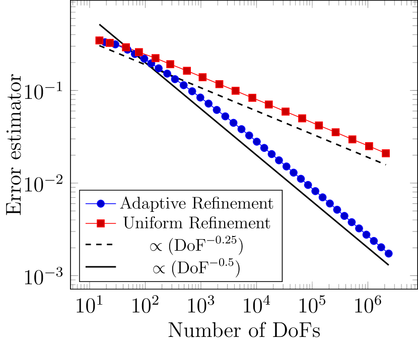
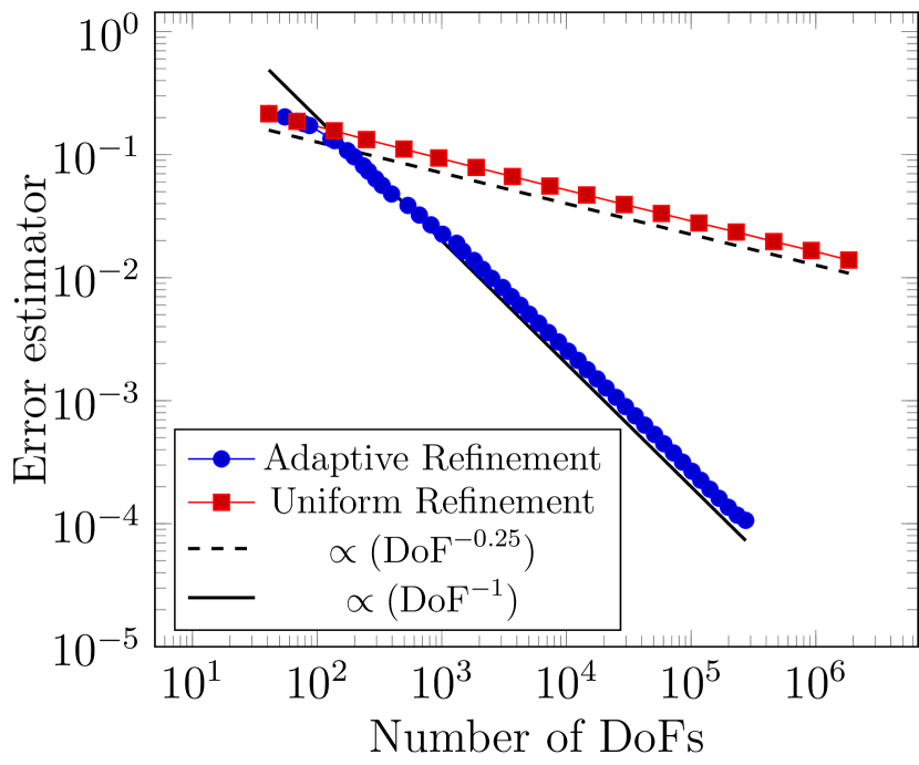
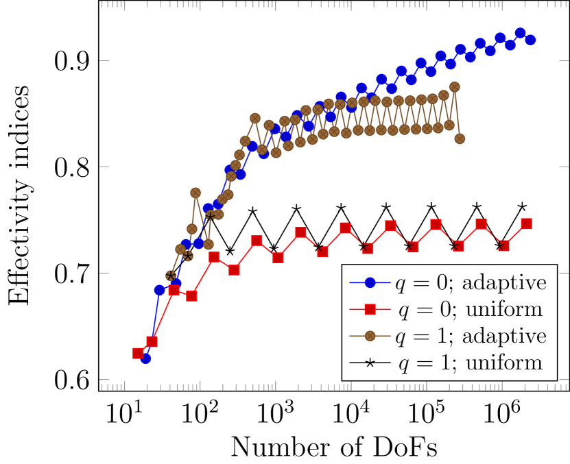
Bottom left: #DoFs in vs. effectivity index .
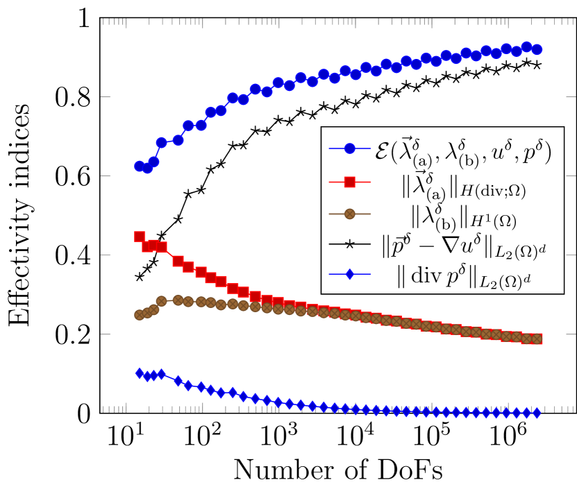
Bottom right: #DoFs in vs. different parts of the error estimator , all multiplied with , for adaptive refinement with .
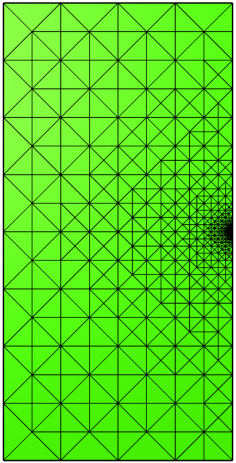
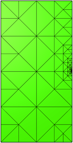
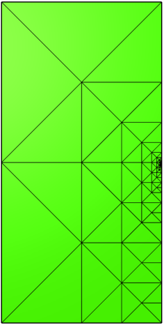
An example of the triangulation , and corresponding triangulations and is given in Figure 2.
7.2. Experiments using Machine Learning
Considering the elliptic model problem
we will compare our newly introduced methods to three prevalent archetypes of Machine Learning approaches: Deep Ritz Method (DRM) [EY18], Physics Informed Neural Network (PINN) [RPK17], and Weak Adversarial Network (WAN) [BYZZ20]. The first of these methods (DRM) minimises the energy functional, the second method (PINN) minimises the squared -norm of the residual, while the latter (approximately) minimises the squared -norm of the residual. All three however deal with the essential boundary condition through the addition of a multiple of the squared -norm of the boundary residual to the functional to be minimised .
In general, all these methods minimise a loss functional over some (deep) neural network , finding an approximate solution . In the aforementioned examples, and the loss functions are as follows
where with , some chosen constant, and a neural network like . Note that in the WAN case, due to the need of evaluating a dual-norm, there is an additional supremum of . For reasons explained in Sect. 6.1, it is best to rewrite the WAN loss function using Lemma 6.3 in the form
We compare above methods with the following four newly introduced least square loss functions whose minimum over the neural network will produce a quasi-best solution from , given that the neural network at the test side is big enough:
(QOLS1Δ) and (QOLS2Δ) are the first order system and second order least squares formulations from (6.2) and (6.3), specialized to the case that , and , and (QOLS1) and (QOLS2) are the corresponding formulations where the Dirichlet boundary condition is enforced by means of (1.1) instead of (1.3).
As with the WAN method, these formulations involve solving a minimax problem. To solve this in practise, one therefore needs to switch between minimising the loss function over the test space for steps, and maximising over the trial space for steps. One might consider a more intelligent switching between minimizing and maximizing, but this is beyond the scope of this paper.
As the given integrals so far will most often not have a closed form, these must be approximated. This can either be done with Monte Carlo integration or quadrature integration, each having its pros and cons.
Monte Carlo integration has two main benefits. Firstly, it induces some stochastic property in our integral, which combined with gradient descent (like) algorithms, gives rise to a stochastic gradient like approach. This makes sure that the solution is not trained to minimise for specific grid points and helps prevent getting stuck in local minima. The second advantage is that the amount of required samples in Monte Carlo methods do not scale exponentially with dimension as opposed to traditional quadrature schemes for which one requires a meshing of the domain, the so-called ‘curse of dimensionality’. We will use simple uniform sampling of the domain for our Monte Carlo integration, which results in the following approximations
where the and are sampled uniformly from their respective domains. It is possible to adopt different sampling strategies to decrease the variance (such as importance sampling [NGM21] or quasi-Monte Carlo strategies [CDLL19]), but this is not the focus of this paper and we will therefore stick to the straightforward uniform sampling.
The other option is to use some sort of quadrature rule to approximate the integrals. Its main advantage is that for smaller dimensions it gives a much better convergence rate, and in general gives more control over the quality of the approximation. Its downsides are that it does not scale well up to higher dimensions and one needs to make it an adaptive scheme to counteract overfitting on the quadrature points [RTOP22]. For the numerical experiments on a domain that is the union of -dimensional hypercubes, an adaptive tensor product Gauss-Legendre quadrature scheme was implemented. This was done by initially subdividing the domain into hypercubes . The scheme was then made adaptive by dividing each into hypercubes , and computing the following criterium
where with we denote the Gauss-Legendre tensor product quadrature of a function over a hypercube . If the criterium holds true, the subdomain is accepted and does not to be refined further, otherwise it is rejected and gets replaced by its refined subdomains. Ideally the refinements stops when all subdomains are accepted, in which case one expects either an absolute error of the order or a relative error of the order , where and are some chosen constants. Unfortunately this can be expensive (i.e. in the case of a singular function ), so for practical reasons the refinements will automatically be stopped after 1000 rejections and consequent refinements of the domain. This checking and refining can be done completely in parallel and can thus be expected to be similarly fast (if not faster due to potentially requiring fewer samples) as Monte Carlo integration if implemented well.
This then leaves us with defining the deep neural networks and in which our trial and test solution will lie. For the architecture of these networks, we have opted for the so-called Residual Neural Networks (ResNet). These were introduced in [HZRS15], and were designed to avoid the vanishing gradient problem, making them easier to train. A graphical representation of the ResNet we used, is given in Figure 3. This network is built out of two main components: the ResNet blocks and linear transformations, one to get the input vector to same width as the ResNet block and one to get the output of the last ResNet block to the correct output dimension.
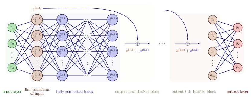
Using the same notation as in Figure 3, the network first calculates
in which and . Note that the notation signifies the ’th layer of the ’th ResNet block. With , we have entered the first ResNet block. This is a fully connected neural network (FCNN) of width and depth . This means that to get from layer to for , one calculates
where , and is some non-linear activation function which acts coordinate wise. To ensure that this architecture does not suffer from a vanishing gradient, the final output of the ’th ResNet block is given by the addition of the first layer of its FCNN with the last
We can therefore define
which maps from the initial layer of the ’th ResNet block, to its output. The last step is a linear transformation from the final ResNet block output to the output vector , which is given by
where and . We therefore find that
| (7.5) |
In the context of neural networks, this function is often called the ‘forward’ function of the network.
The set of all possible different parameters of our ResNet will be denoted with
This allows us to define our neural network space of functions as
where denotes the forward function as defined in (7.5) for a specific choice of parameters . Note that the number of degrees of freedom for our ResNet is given by .
Having now defined all necessary components, we can formulate the general algorithm for solving our model problem
This algorithm was implemented for each of the different QOLS formulations along with the DRM, WAN and PINN in Python using PyTorch.
Example 7.1.
To compare these methods we will look at the following problem
with the L-shaped domain . Note that the exact solution is only in for , with its gradient blowing up at the origin. Because of the non-smoothness of at we expect that our correct imposition of the boundary condition will show-off.
The networks for and in each of the different methods are chosen to be , where is either or , depending on the required amount of outputs, which yields , and degrees of freedom respectively. The activation function between all layers is chosen to be the Exponential Linear Unit (ELU), as it is a smooth function guaranteeing that and .
For the methods (WAN, QOLS2, QOLS2Δ) that require a , one could define it to be the exact distance to the boundary but this will result in a with being discontinuous, which can lead to numerical integration issues. Instead we will define as
for , where the are the exact distance functions to each of the sides of our domain . With this definition, one finds that and [SS22].
For backward propagation of the models ( and ), we will use the popular AdamW algorithm for gradient descent, with the learning rate set to the recommended . For the QOLS methods, we let the learning rate drop off slowly by multiplying it with every epochs (resulting in a learning rate of approximately at the end). We do this as we found experimentally that these methods already reach a local minimum very rapidly for , and decreasing the learning rate somewhat helps stabilize them.
For the numerical integration, in the case of Monte Carlo integration we set and , while for the adaptive quadrature we used Gauss-Legendre integration with polynomial degree , an initial subdivision of into subdomains, a maximum of further refinements and tolerances .
Lastly we ran all methods for epochs, chose and, for the existing machine learning approaches, set the parameter . This choice for seems to be a pretty optimal choice from experiments. The results using adaptive quadrature integration are presented in Figure 4 and are very similar to the results using Monte Carlo integration, the main difference being that the former managed an extra decrease in -error of about 2-4 time for the smallest -errors.
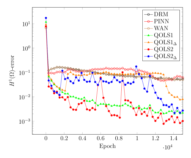
From these results we find that for this problem our newly introduced QOLS formulations outperform the DRM, PINN and WAN methods. It could be that given enough epochs, these methods catch up, but at least on this time scale for similar learning rates the QOLS formulations perform (up to 100x) better. For smooth problems (e.g. ) the performance gap as in Figure 4 is much less prevalent if present at all.
Comparing the QOLS methods among themselves, we find the first order system formulations slightly outperforming the second order formulations. This does come at the price of needing vector-valued functions within the trial space possibly necessitating more network parameters for higher dimensional problems to model these extra outputs. Furthermore we find that the formulations slightly underperform compared to their counterparts, but one can expect for the aforementioned reasons that for higher dimensional problems this will turn around as the formulations have scalar-valued functions in their test space .
On a practical note, the QOLS formulations have the advantage of not having to bother with making a good choice for , a choice which greatly affects the performance of the DRM, PINN and WAN methods that can only be attained empirically. A downside however is that the QOLS formulations, similar to WAN, have to deal with an adversarial network and solve a min-max problem as a result of minimizing a dual norm. This is a lot more expensive and as far as we know, there is no intelligent way of choosing when to switch between the inner and outer loop.
8. Conclusion
We have introduced least-squares formulations of second order elliptic equations and the stationary Stokes equations with possibly inhomogeneous boundary conditions, whose minimization over a finite element space or a Neural Net yield approximations that are quasi-best. This is due to the fact that the least-squares residual is equivalent to the (squared) error in a canonical norm. Despite of that, the use of fractional Sobolev norms on the boundary, or even any function space on the boundary has been avoided. Such spaces were replaced by the ranges of trace operators of standard function spaces on the domain. Some parts of the residual are measured in dual norms. For sufficiently large test finite element spaces or adversarial Neural Nets, they are replaced by discretized dual norms whilst preserving quasi-optimal approximations. Numerical results both for finite element spaces and for Neural Nets are presented. The advantage of our approach compared to usual Machine Learning algorithms is apparent for solutions that have singularities. It is however fair to say that known problems with Machine Learning algorithms for solving PDEs, as quadrature issues or the painful minimization of a non-convex functional, are not solved by the use of our well-posed least-squares functionals.
Appendix A Proof of Proposition 5.1
By testing the first and second equation of this system with and , respectively, and applying integration by parts we obtain
From , and so on , regardless of the boundary datum the Stokes solution satisfies
| (A.2) |
(). The operator defined by the left hand side is in . Furthermore, it is well-known that this operator is in .
To arrive at a first order system, we introduce the vorticity as an additional variable. Then (A.2) is equivalent to the system
| (A.3) |
(). With , , and , the operator defined by the left hand side, which we will denote by , satisfies . To see that , replace the zero at the right hand side of the second equation by . By substituting in the first equation, by the well-posedness of (A.2) one finds a solution whose norm is bounded by the norm of the data in .
A solution of (A.3) satisfies . Since satisfies , we conclude that
| (A.4) |
(). The operator defined by the left hand side, which we will denote by , satisfies . The squared norm reads as
and reads as
From , applications of the triangle inequality show . From , it follows that for , , i.e., is a homeomorphism with its range. For arbitrary , there exists a , with , and so , meaning that .
Finally, as we have seen, a consistent formulation of Stokes problem with for , with , is given by
It holds that , is surjective, with kernel equal to , and . By an application of Lemma 3.3 we conclude that .
References
- [BBH23] S. Bertoluzza, E. Burman, and C. He. Wan discretization of pdes: best approximation, stabilization and essential boundary conditions, 2023.
- [BBO03] I. Babuška, U. Banerjee, and J.E. Osborn. Survey of meshless and generalized finite element methods: a unified approach. Acta Numer., 12:1–125, 2003.
- [BDD04] P. Binev, W. Dahmen, and R. DeVore. Adaptive finite element methods with convergence rates. Numer. Math., 97(2):219 – 268, 2004.
- [BG09] P.B. Bochev and M.D. Gunzburger. Least-squares finite element methods, volume 166 of Applied Mathematical Sciences. Springer, New York, 2009.
- [BM24] M. Bernkopf and J. M. Melenk. Optimal convergence rates in for a first order system least squares finite element method—part II: Inhomogeneous Robin boundary conditions. Comput. Math. Appl., 173:1–18, 2024.
- [BS15] D. Broersen and R. P. Stevenson. A Petrov-Galerkin discretization with optimal test space of a mild-weak formulation of convection-diffusion equations in mixed form. IMA J. Numer. Anal., 35(1):39–73, 2015.
- [BYZZ20] G. Bao, X. Ye, Y. Zang, and H. Zhou. Numerical solution of inverse problems by weak adversarial networks. Inverse Problems, 36(11):115003, 31, 2020.
- [CCLL20] Z. Cai, J. Chen, M. Liu, and X. Liu. Deep least-squares methods: an unsupervised learning-based numerical method for solving elliptic PDEs. J. Comput. Phys., 420:109707, 13, 2020.
- [CDLL19] J. Chen, R. Du, P. Li, and L. Lyu. Quasi-monte carlo sampling for machine-learning partial differential equations, 2019.
- [CMM95] Z. Cai, T. A. Manteuffel, and S. F. McCormick. First-order system least squares for velocity-vorticity-pressure form of the Stokes equations, with application to linear elasticity. Electron. Trans. Numer. Anal., 3(Dec.):150–159 (electronic), 1995.
- [EGSV22] A. Ern, Th. Gudi, I. Smears, and M. Vohralík. Equivalence of local- and global-best approximations, a simple stable local commuting projector, and optimal approximation estimates in . IMA J. Numer. Anal., 42(2):1023–1049, 2022.
- [EY18] W. E and B. Yu. The deep Ritz method: a deep learning-based numerical algorithm for solving variational problems. Commun. Math. Stat., 6(1):1–12, 2018.
- [Füh24] Th. Führer. On a Mixed FEM and a FOSLS with Loads. Comput. Methods Appl. Math., 24(2):355–370, 2024.
- [Gri85] P. Grisvard. Elliptic problems in nonsmooth domains, volume 24 of Monographs and Studies in Mathematics. Pitman (Advanced Publishing Program), Boston, MA, 1985.
- [GS21] G. Gantner and R.P. Stevenson. Further results on a space-time FOSLS formulation of parabolic PDEs. ESAIM Math. Model. Numer. Anal., 55(1):283–299, 2021.
- [HZRS15] K. He, X. Zhang, S. Ren, and J. Sun. Deep residual learning for image recognition. 2016 IEEE Conference on Computer Vision and Pattern Recognition (CVPR), pages 770–778, 2015.
- [Kat60] T. Kato. Estimation of iterated matrices, with application to the von Neumann condition. Numer. Math., 2:22–29, 1960.
- [KLS23] C. Köthe, R. Löscher, and O. Steinbach. Adaptive least-squares space-time finite element methods, 2023.
- [LCR23] M. Liu, Z. Cai, and K. Ramani. Deep Ritz method with adaptive quadrature for linear elasticity. Comput. Methods Appl. Mech. Engrg., 415:Paper No. 116229, 16, 2023.
- [LM21] Y. Liao and P. Ming. Deep Nitsche method: deep Ritz method with essential boundary conditions. Commun. Comput. Phys., 29(5):1365–1384, 2021.
- [MSS24] H. Monsuur, R.P. Stevenson, and J. Storn. Minimal residual methods in negative or fractional Sobolev norms. Math. Comp., 93(347):1027–1052, 2024.
- [NGM21] M. Nabian, R. Gladstone, and H. Meidani. Efficient training of physics-informed neural networks via importance sampling. Computer-Aided Civil and Infrastructure Engineering, 36(8):962–977, 2021.
- [Nit68] J. Nitsche. Ein Kriterium für die Quasi-Optimalität des Ritzsches Verfahrens. Numer. Math., 11:346–348, 1968.
- [OPS24] J. Opschoor, P. Petersen, and Ch. Schwab. First order system least squares neural networks, 2024.
- [RPK17] M. Raissi, P. Perdikaris, and G.E. Karniadakis. Machine learning of linear differential equations using Gaussian processes. J. Comput. Phys., 348:683–693, 2017.
- [RTOP22] J. Rivera, J. Taylor, Á. Omella, and D. Pardo. On quadrature rules for solving partial differential equations using neural networks. Computer Methods in Applied Mechanics and Engineering, 393:114710, 2022.
- [SS22] N. Sukumar and A. Srivastava. Exact imposition of boundary conditions with distance functions in physics-informed deep neural networks. Comput. Methods Appl. Mech. Engrg., 389:Paper No. 114333, 50, 2022.
- [Sta99] G. Starke. Multilevel boundary functionals for least-squares mixed finite element methods. SIAM J. Numer. Anal., 36(4):1065–1077 (electronic), 1999.
- [Ste08] R.P. Stevenson. The completion of locally refined simplicial partitions created by bisection. Math. Comp., 77:227–241, 2008.
- [Ste14] R.P. Stevenson. First-order system least squares with inhomogeneous boundary conditions. IMA J. Numer. Anal., 34(3):863–878, 2014.
- [Ste23] R.P. Stevenson. A convenient inclusion of inhomogeneous boundary conditions in minimal residual methods. Computational Methods in Applied Mathematics, 2023.
- [SW21] R.P. Stevenson and J. Westerdiep. Minimal residual space-time discretizations of parabolic equations: Asymmetric spatial operators. Comput. Math. Appl., 101:107–118, 2021.
- [SY21] H. Sheng and C. Yang. PFNN: a penalty-free neural network method for solving a class of second-order boundary-value problems on complex geometries. J. Comput. Phys., 428:Paper No. 110085, 13, 2021.
- [SZ90] L. R. Scott and S. Zhang. Finite element interpolation of nonsmooth functions satisfying boundary conditions. Math. Comp., 54(190):483–493, 1990.
- [XZ03] J. Xu and L. Zikatanov. Some observations on Babuška and Brezzi theories. Numer. Math., 94(1):195–202, 2003.