Temporally Compressed 3D Gaussian Splatting for Dynamic Scenes

Abstract

Recent advancements in high-fidelity dynamic scene reconstruction have leveraged dynamic 3D Gaussians and 4D Gaussian Splatting for realistic scene representation. However, to make these methods viable for real-time applications such as AR/VR, gaming, and rendering on low-power devices, substantial reductions in memory usage and improvements in rendering efficiency are required. While many state-of-the-art methods prioritize lightweight implementations, they struggle in handling scenes with complex motions or long sequences. In this work, we introduce Temporally Compressed 3D Gaussian Splatting (TC3DGS), a novel technique designed specifically to effectively compress dynamic 3D Gaussian representations. TC3DGS selectively prunes Gaussians based on their temporal relevance and employs gradient-aware mixed-precision quantization to dynamically compress Gaussian parameters. It additionally relies on a variation of the Ramer-Douglas-Peucker algorithm in a post-processing step to further reduce storage by interpolating Gaussian trajectories across frames. Our experiments across multiple datasets demonstrate that TC3DGS achieves up to 67$\times$ compression with minimal or no degradation in visual quality.

1 Introduction

Dynamic scene reconstruction is essential for applications in virtual and augmented reality, gaming and robotics, where a real-time and accurate representation of moving objects and their environment is key to immersive experiences. Recent advancements such as Neural Radiance Fields (NeRF) [28] have enabled high-fidelity scene generation, albeit at the cost of slow rendering speeds. To address this limitation, 3D Gaussian Splatting (3DGS) [20] leverages sparse Gaussian splats for efficient scene rendering, particularly for static scenes.

Since the advent of 3DGS, a plethora of extensions to dynamic scenes have been proposed [39, 26, 6, 40, 41, 8]. In this context, some methods [39, 26, 6, 40] allow the Gaussians to evolve over time, capturing time-varying properties such as position, opacity, and covariance. In contrast, other methods learn spatio-temporal Gaussians to represent the dynamic content directly, which allows for a more flexible modeling of scene variations [6, 40, 8, 41]. However, obtaining a high-quality representation with these methods often requires a large number of Gaussians, leading to substantial storage overhead. Furthermore, as shown in Figure 2, spatio-temporal methods face the challenge of effectively adjusting the Gaussian parameters when applied to dynamic scenes with rapid and complex motions, such as those in [18]. This is alleviated by Dynamic 3D Gaussians [26], which enforces consistency across all frames, but at the cost of increased storage and rendering time.

To address these challenges, we propose Temporally Compressed 3D Gaussian Splatting (TC3DGS), a novel approach designed to efficiently compress dynamic 3D Gaussian representations for high-quality, real-time scene rendering. Unlike traditional methods, TC3DGS reduces both the number and the memory footprint of the Gaussians, by selectively pruning splats based on temporal importance and learning a parameter-specific bit-precision. This selective compression allows us to maintain scene fidelity while significantly reducing storage and computational requirements, making TC3DGS well-suited for dynamic environments with complex motions.

Our approach begins with a pruning and masking strategy designed to eliminate redundant Gaussians. While previous works [42, 11, 21] have proposed pruning methods for 3DGS, they do not attempt to model dynamic scenes and thus take no advantage of temporal compression. Unfortunately, adapting these pruning strategies to dynamic scenes is not straightforward, as different Gaussians may need to be pruned across different frames. Here, we introduce a method that explicitly integrates this temporal aspect into the training objective, allowing us to prune dynamic Gaussian splats more effectively. To further optimize memory usage in our scene representation, we also aim to compress the storage size of the remaining Gaussians. To this end, we developed a gradient-aware mixed-precision quantization method that adjusts the bit precision of each Gaussian parameter based on its sensitivity. We use gradient magnitudes to determine parameters with high sensitivity, and allocate them a higher precision, while those with lower impact on the scene are quantized with fewer bits. Therefore, our method achieves a good balance between compression and reconstruction accuracy. Finally, to further enhance the efficiency of our dynamic representation, we introduce a keypoint extraction algorithm as a post-processing step. This algorithm simplifies the temporal trajectories of the Gaussian parameters, preserving only the key data points that are crucial for accurate dynamic scene representation. This greatly reduces the amount of temporal data stored, allowing for more compact scene representations, as demonstrated in our experiments where we achieve a compression rate of up to 67$\times$ while preserving rendering quality.

Our experiments on benchmark datasets demonstrate the benefits of our method across diverse scenarios. Furthermore, we perform an ablation study to demonstrate the contribution of each key component in our pipeline. In a nutshell, our major contributions are as follows:

• We introduce the first method to prune dynamic Gaussian splats, going beyond previous pruning techniques, designed for static scenes, by incorporating temporal relevance into the pruning process.

• We develop a sensitivity-driven, gradient-based quantization method that dynamically assigns bit precision to parameters based on their impact on reconstruction accuracy, optimizing memory usage.

• We propose a keypoint extraction post-processing algorithm to further reduce storage requirements by simplifying the Gaussian parameter trajectories, retaining only essential data points for compact scene representations.

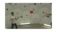
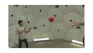
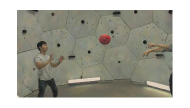
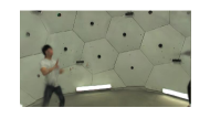
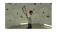
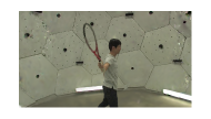
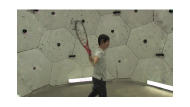
Ground Truth	Dynamic 3DGS [26]	TC3DGS (Ours)	STG [23]	4D Gaussian [38]

Figure 2: Comparative Evaluation on Panoptic Dataset [18] Recent lightweight state-of-the-art methods (STG [23], and 4D-Gaussian [38]) struggle to accurately reconstruct scenes in complex environments. In contrast, our compression strategy effectively captures and maintains high fidelity in dynamic scene details.

2 Related Work

Dynamic 3D reconstruction.

Recent advancements in 3D reconstruction based on Neural Radiance Fields (NeRFs) [28] and 3D Gaussian Splatting (3DGS) [20] have achieved remarkable levels of visual fidelity and accuracy. These methods have subsequently been extended to 4D representations [33, 24, 13], enabling dynamic scene reconstruction. Methods to decompose a 4D scene into multiple 2D planes to learn a more compact representation are also explored by various methods [16, 3, 35, 1]. In the case of 3DGS, where Gaussians are explicitly stored and rendered, different approaches have emerged to model their time dependence. One prominent line of work [39, 26, 6, 40] in this area optimizes a canonical set of Gaussians from the initial frame, and combines it with a deformation motion field allowing temporal variations of the Gaussian parameters. However, these methods are limited to short videos, as they cannot add Gaussians after the initial frame.

Another class of methods [41, 8, 19, 9] directly models temporal Gaussians that can be present in a subset of frames, enabling certain elements to appear in selected time ranges and thus increasing the expressivity of their reconstruction. However, a major limitation across these methods is that both training and inference times for novel view synthesis scale with the number of Gaussians, the length of the sequence, and the complexity of their parameters, presenting a key bottleneck in enhancing reconstruction quality.

Compressed 3D radiance fields.

An important research direction has thus emerged in developing more compact representations of radiance fields. For NeRFs, compact grid structures [30, 4, 15, 14] have already proven effective in reducing network sizes and enhancing accuracy.

With 3DGS, recent works have either concentrated on optimizing the representation of the Gaussian parameters [11], or on identifying low-importance Gaussians and pruning them entirely [42, 11, 21]. Unorthodox techniques like representing the Gaussian parameters as 2D grids and applying image compression techniques [29, 31] have also been studied. Better initialization and weighted sampling based pruning [12] has also shown promising results. Additionally, the use of traditional compression techniques such as vector quantization [21, 31] or entropy models [5] have shown some potential for the compression of static scenes, but scaling them to dynamic scenes with possibly hundreds or thousands of frames remains a challenge.

Indeed, dynamic scenes require an even larger set of parameters to accurately capture motion, temporal variations, and complex interactions within the scene.

The temporal relevance of each Gaussian changes dynamically, and traditional pruning strategies designed for static scenes are insufficient, as they lack adaptability to these fluctuations. To the best of our knowledge, we are the first to propose a compression framework specifically designed for dynamic 3D Gaussians. Our approach combines temporal relevance-based pruning, gradient-based mixed-precision quantization, and trajectory simplification to address the unique requirements of dynamic scenes.

3 Method

In this section, we will first briefly discuss the Dynamic 3DGS [26] method in Sec. 3.1, which serves as the foundation of our proposed approach. We then detail in Sec. 3.2.1 our novel masking and pruning strategies designed to eliminate redundant Gaussians. Next, we present a sensitivity-based mixed precision technique for efficient parameter compression in Sec. 3.2.2, followed by a post-training compression strategy aimed at minimizing storage overhead in Sec. 3.2.3.

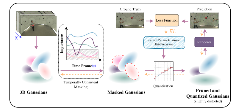
Figure 3: Overview of our Temporally Compressed 3D Gaussian Splatting for Dynamic Scenese (TC3DGS) method. Our approach involves a temporally consistent masking strategy to select relevant 3D Gaussians across frames. The masked Gaussians are then pruned and quantized using a gradient-based, parameter-aware bit-precision quantization scheme, which optimizes memory usage while preserving scene fidelity.

3.1 Dynamic 3D Gaussians

Dynamic 3DGS [26] models dynamic scenes by allowing the Gaussians to move and rotate over time while enforcing that they have persistent color, opacity, and scale. This approach reconstructs a dynamic 3D scene over time using a series of images taken from multiple cameras across different time steps, along with the cameras’ intrinsic and extrinsic parameters. The method sequentially reconstructs a dynamic 3D scene by initializing each time step from the previous one and performing test-time optimization without additional training data. This is unlike most other concurrent methods, which attempt to optimize all frames jointly. This conceptual difference allows Dynamic 3DGS [26] to enforce consistency in the reconstructed Gaussians across frames. Additionally, this method enables tracking objects throughout the dynamic scene, as each 3D Gaussian has a unique correspondence across frames.

Each dynamic scene $\mathcal{S}$ is parameterized by a set of Dynamic 3D Gaussians, with certain parameters fixed for the entire sequence and others varying over time. Specifically, each Gaussian retains a fixed 3D scale $(s_{x},s_{y},s_{z})$, color $(r,g,b)$, opacity logit $o$, and background logit $bg$ as determined in the initial frame. In contrast, parameters such as the 3D center $(x_{t},y_{t},z_{t})$ and 3D rotation, expressed as a quaternion $(q_{w,t},q_{x,t},q_{y,t},q_{z,t})$, evolve over time. This formulation enables the Gaussians to represent consistent scene elements across frames while dynamically adjusting their positions and orientations.

During training, this 3D scene representation is iteratively updated using a differentiable renderer to minimize the photometric error between the rendered and input images. Specifically, each Gaussian influences a point $p$ in physical 3D space according to the standard (unnormalized) Gaussian equation weighted by its opacity, i.e.,

$$f_{i,t}(p) =\sigma({o_{i}})\exp\left(-\frac{1}{2}(p-\mu_{i,t})^{T}\Sigma_{i,t}^{-1}(p-\mu_{i,t})\right)\;,$$

where ${\mu}_{i,t}=\begin{bmatrix}x_{i,t}&y_{i,t}&z_{i,t}\end{bmatrix}^{T}$ is the center of Gaussian $i$ at timestep $t$, and $\Sigma_{i,t}=R_{i,t}S_{i}S_{i}^{T}R_{i,t}^{T}$ is the covariance matrix of Gaussian $i$ at timestep $t$, obtained by combining the scaling matrix $S_{i}=\text{diag}\left(\begin{bmatrix}s_{x,i}&s_{y,i}&s_{z,i}\end{bmatrix}\right)$, and the rotation component $R_{i,t}=\textrm{q2R}\left(\begin{bmatrix}q_{w_{i,t}}&q_{x_{i,t}}&q_{y_{i,t}}&q_{z_{i,t}}\end{bmatrix}\right)$, where $\textrm{q2R}()$ constructs a rotation matrix from a quaternion. Finally, $\sigma$ is the standard sigmoid function.

3.2 TC3DGS

Dynamic 3DGS [26] is particularly promising because it models the dynamic scene as movements of Gaussians under kinematic constraints w.r.t. the previous timestep. By optimizing the position and rotation of the Gaussians instead of learning deformation functions, it removes the limitation on possible deformations due to the characteristics of the modeling function. However, by learning position and rotation at each timestep separately, the number of parameters increases linearly, resulting in large storage sizes, and thus limiting its applicability to high-fidelity and long-range scene modeling.

3.2.1 Gaussian Masking and Pruning

Pruning techniques aimed at identifying and removing low-importance Gaussians have been successfully applied to static 3D Gaussian splatting [21, 32, 17, 11]. However, for dynamic scenes, a temporally consistent importance measure is required to ensure that the pruned Gaussians remain insignificant throughout the scene’s duration.

Various approaches to computing the importance of each Gaussian in static scenes using training images and camera positions have bee proposed [32, 11]. These methods focus on the contribution of each Gaussian to the training views. In dynamic scenes, Gaussians are not stationary, so their contributions vary over time. To prune Gaussians effectively from dynamic scenes, it is essential to maintain the contributions of high-importance Gaussians consistently high, while suppressing low-importance ones, thus enabling more effective pruning.

Compact-3DGS [21] introduces a masking approach based on Gaussian volume and transparency. Gaussians with low opacity, minimal volume, or both are masked out since they have negligible impact on the rendered images. A mask parameter $m\in\mathbb{R}^{N}$ is learned to produce binary masks $M\in\{0,1\}^{N}$ using a straight-through estimator. This binary mask is then applied to the Gaussians by scaling their opacities and sizes. This is expressed as

$$M_{n} =\operatorname*{sg}(\mathds{1}[\sigma(m_{n})>\epsilon]-\sigma(m_{n}))+\sigma(m_{n}),$$ (1)

$$\hat{s}_{n} =M_{n}s_{n},\quad\hat{o}_{n}=M_{n}o_{n},$$ (2)

where $n$ represents the Gaussian index, $\epsilon$ denotes the masking threshold, $\operatorname*{sg}(\cdot)$ is the stop-gradient operator, and $\mathds{1}[\cdot]$ and $\sigma(\cdot)$ correspond to the indicator and sigmoid functions, respectively.

Compact-3DGS [21] explains that this mask learns to remove Gaussians with low opacity and/or small volume. However, as shown in Figure 4, this explanation does not hold in dynamic scenes. The value of $m_{n}$ can change significantly across time frames, even with fixed opacity $o$ and scale $s$ after the initial time frame.

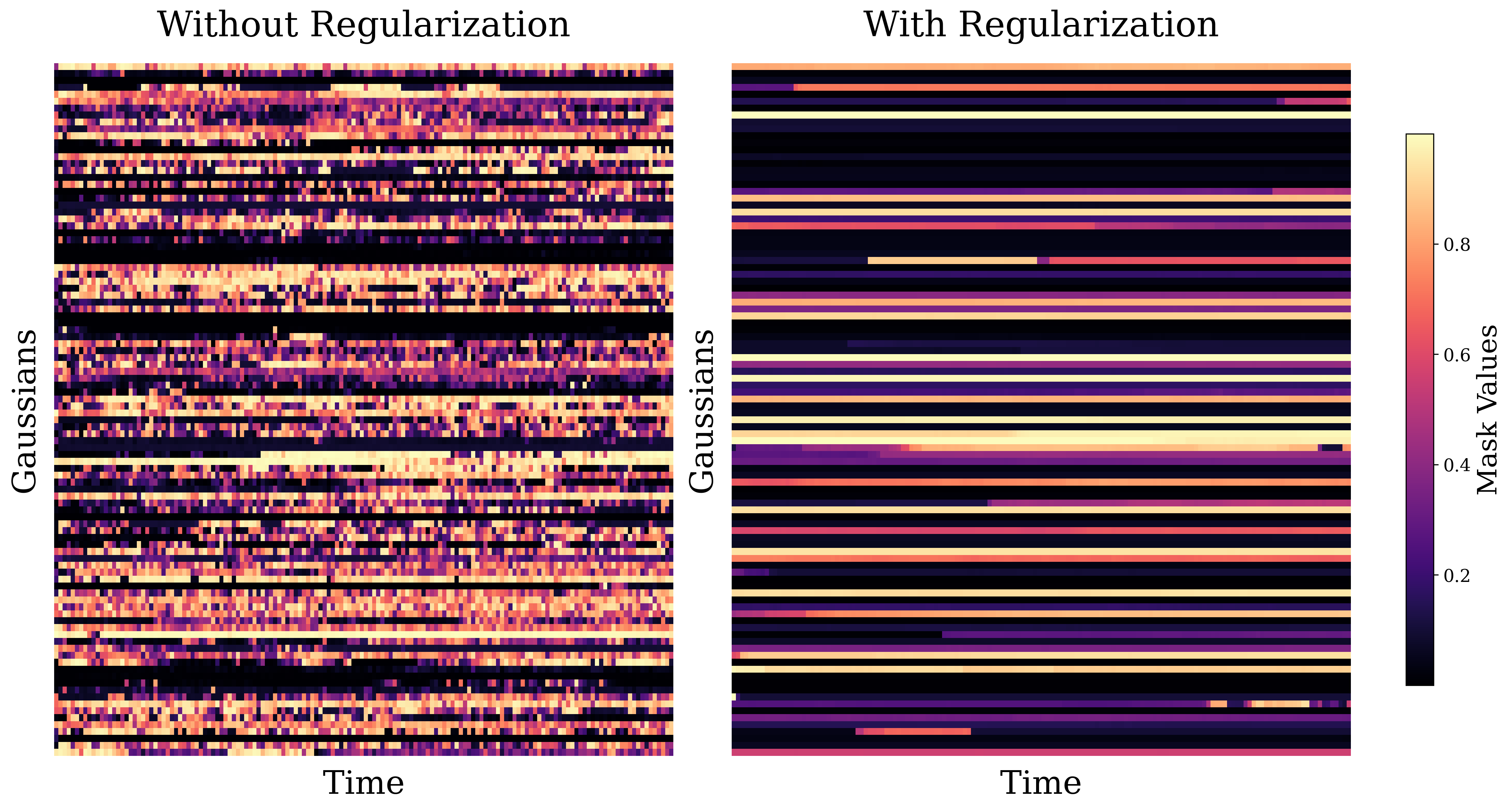
Figure 4: Mask Consistency. (Left) Mask values of Gaussians trained independently for each time frame. (Right) Mask values trained with our loss.

In dynamic scenes, $m_{n}$ depends on the 2D projected area of the Gaussians in the training views and their transmittance, where transmittance $T_{i}$ for the $i^{th}$ Gaussian along a camera ray is defined as the Gaussian’s contribution to blending, i.e.,

$$T_{i}=\sigma(o_{i})\prod_{j=1}^{i-1}(1-\sigma(o_{j})).$$ (3)

As a Gaussian moves relative to the others, changes in $T_{i}$ are reflected in $m_{n}$. Similarly, when a Gaussian moves toward or away from the training cameras, its projected area in the views changes, affecting $m_{n}$ accordingly.

Since the values in $m$ strictly need to be high due to their role in rendering through Eq. 1 and the photometric loss, we introduce an additional regularization to incentivize lower values. We thus regularize $m$ by minimizing

$$\mathcal{L}_{mask}=\sum_{n=1}^{N}\sigma(m_{n}).$$ (4)

This regularization loss penalizes unnecessarily high values, reducing $m$ to the minimum required to produce satisfying renderings. The flexibility of this learned mask is one of its key advantages, as it can be optimized to exhibit desired properties via the use of additional constraints.

A key motivation for ensuring consistency of $m_{n,t}$ across frames is to capture the global importance of the Gaussians during pruning. To achieve this, we learn $m_{n,t}$ for each timestamp and introduce a consistency loss function that encourages $m_{n,t}$ to remain close to $m_{n,t-1}$. Specifically, we define this mask consistency loss function as

$$\mathcal{L}_{mc}=\sum_{n=1}^{N}|m_{n,t}-sg(m_{n,t-1})|.$$ (5)

It ensures that the masks exhibit stability across the frames, as shown in Figure 4 (Right). By maintaining consistency, our approach prevents sudden fluctuations in Gaussian importance, which can degrade rendering quality and lead to suboptimal pruning results.

After optimizing across all timestamps, we perform Gaussian pruning based on the average value of $m_{n}$. Specifically, a Gaussian is pruned if its average value across all timestamps satisfies

$$\frac{1}{T}\sum_{t=1}^{T}\sigma(m_{n,t})<\epsilon.$$ (6)

3.2.2 Gradient-Aware Mix-Precision Quantization

The influence of the Gaussian parameters on reconstruction quality is highly variable; a small adjustment in one parameter can significantly alter the rendered image, whereas similar adjustments in other parameters or in the same parameter of a different Gaussian may have minimal impact. Our approach uses gradient-based sensitivities to dynamically assign bit precision to each parameter, based on its influence on reconstruction accuracy. By leveraging this adaptive, in-optimization quantization, each parameter adjusts its quantization scale [10] in real-time, preserving detail in the reconstructed scene.

We first calculate the mean sensitivity for each parameter based on the gradients [43, 32], reflecting each parameter’s impact on the image reconstruction performance. We introduce a sensitivity coefficient $S(\theta)$, which represents the responsiveness of image quality $Q$ to changes in a Gaussian parameter $\theta$. This coefficient is formulated as

$$S(\theta) =\frac{1}{\sum_{k=1}^{K}N_{k}}\sum_{k=1}^{K}\big{|}\frac{\partial Q_{k}}{\partial\theta}\big{|}.$$ (7)

where $K$ is the total number of training images used for reconstruction, $N_{k}$ is the number of pixels in the $k^{th}$ image, and $Q_{m}$ denotes the cumulative pixel intensity across the RGB channels in image $k$, serving as a proxy for image quality.

The coefficient $S(\theta)$ quantifies how sensitive $Q$ is to variations in $\theta$, measured by the gradient $\frac{\partial Q}{\partial\theta}$. A higher gradient indicates that small adjustments in $\theta$ yield large changes in image quality, suggesting a greater impact of $\theta$ on the reconstruction.

By using this impact-based metric, we can effectively rank the parameters by their importance on image fidelity. We then normalize each sensitivity coefficient by scaling it based on the minimum and maximum co-efficient across all parameters. This standardization ensures that all the coefficients fall within a consistent range.

Using the normalized sensitivity $\gamma\in[0,1]$, we assign a dynamic bit precision $b$ within a range of bits $b\in[b_{\text{min}},b_{\text{max}}]$, where $b\in\mathbb{Z}$ is calculated as

$$b=\left\lfloor\gamma\cdot(b_{\text{max}}-b_{\text{min}})\right\rfloor+b_{\text{min}}.$$ (8)

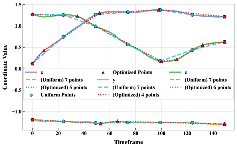
Figure 5: Keypoint Interpolation. In this example, we represent a position across 150 frames with only 5, 4 and 6 keypoints for $x$, $y$ and $z$, respectively, with only $0.038$ MSE. By comparison, uniformly sampling 7 keypoints increases storage and increases error to $0.089$ MSE.

This approach allocates higher bit precision to more sensitive parameters and lower bit precision to less sensitive ones, optimizing the balance between computational efficiency and model accuracy.

After running our scene reconstruction process for a specified number of iterations, we apply mixed-precision quantization to all Gaussian parameters, excluding the position parameter, to achieve low-bit precision for the other parameters. Instead of relying on traditional vector quantization (VQ) or basic min-max quantization, we propose a parameter quantization technique with learnable scaling factors [10], integrating it directly into the optimization process rather than treating it as a post-optimization fine-tuning step. Consequently, many parameters can be effectively quantized to even 4-bit precision, reducing memory and computational load without compromising reconstruction quality.

Training. We train the Gaussian parameters to model the scene one time frame at a time. Following [26], we use physically-based priors to regularize the Gaussians. The optimization objective is defined as

$$\mathcal{L}=\mathcal{L}_{original}+\lambda_{mask}\mathcal{L}_{mask}+\lambda_{mc}\mathcal{L}_{mc},$$ (9)

where $\mathcal{L}_{original}$ is the same loss function as in [26], while $\mathcal{L}_{mask}$ and $\mathcal{L}_{mc}$ are defined in Eq. 4 and 5, respectively.

Algorithm 1 Keypoint Selection

Input: values, max_keypoints ($max_{kp}$), tolerance ($\tau$)

1:Initialize keypoints at first and last positions

2:for $i=1$ to $max_{kp}-2$ do

3:  Compute interpolated values based on keypoints

4:  Compute error for every value

5:  Compute error (mse) for entire sequence

6:  if mse $\leq\tau$ or $|$keypoints$|\geq max_{kp}$ then

7:   break

8:  end if

9:  Select the value with the highest error and add it to keypoints

10:end for

3.2.3 Keypoint Interpolation

Previous implementations of dynamic 3DGS often model the time-dependence of parameters by fitting polynomials to the Gaussian parameters, which greatly limits the range of motions that can accurately be modeled. By contrast, Dynamic 3DGS [26] opts for inefficiently storing all time-dependent parameters, such as Gaussian means, rotations, and colors, for all time frames. While this greatly increases the expressivity of this method compared to other works, it comes at a significant cost in memory.

We take a different approach and observe that only a small subset of keypoints are required to accurately reconstruct complex motions. However, the placement of these keypoints across time cannot be predetermined, as it depends on the individual Gaussians. For instance, background Gaussians require a single keypoint to cover the whole sequence, whereas moving objects will need substantially more keypoints. This motivates the development of our keypoint selection strategy, which we adapt from the Ramer–Douglas–Peucker (RDP) algorithm [7]. It is applied as a post-processing step to further reduce storage requirements for the Gaussian parameters that change over time in dynamic scenes.

While the RDP algorithm selects keypoints from a sequence based on a local error tolerance, $\xi$, we propose a novel keypoint selection method, as outlined in Algorithm 1 . This method offers several advantages over the RDP algorithm. It provides greater flexibility by allowing control via both an acceptable tolerance value, $\tau$, and a maximum number of keypoints. The parameter $\tau$ defines the maximum allowable Mean Squared Error (MSE) over the sequence. Unlike RDP, which is solely controlled by $\xi$, our method enables a hard maximum bound on the number of keypoints, allowing for more precise, fine-grained control.

Following this, we flatten and transpose the time-dependent parameters from $\mathbb{R}^{T\times N\times D}$ to $\mathbb{R}^{ND\times T}$, transforming the data into $ND$ sequences of length $T$. We then compute the keypoints for all Gaussians in parallel, forming sparse matrices. The sparsity of these matrices is controlled using the parameters $max_{kp}$ and $\tau$, and and we store these sparse matrices to minimize memory usage. Upon loading the scene data, we interpolate the keypoints across all timesteps to reconstruct the dense matrices, which are then reshaped to their original parameter dimensions.

4 Experiments

We compare our method with multiple techniques extending the 3D Gaussians approach to dynamic scenes. We evaluate the methods on diverse datasets covering different real-world and synthetic scenarios. Results on additional datasets are provided in the supplementary material along with more visualizations.

4.1 Datasets

4.1.1 Panoptic Sports Dataset

We evaluate our method on the Panoptic Sports dataset, a subset from the Panoptic Studio dataset [18]. This dataset contains 6 different scenes, each having 31 camera sequences spanning 150 frames. We use 4 cameras (0, 10, 15 and 30) for testing and the rest for training, following the convention set by [26]. In addition to the images, we use the provided foreground/background segmentation to apply a segmentation loss to improve the results and prevent the background from moving. This dataset contains complex motions with objects moving quickly and over long distances.

Table 1: Quantitative results on the Panoptic dataset. The best result is shown in bold, while the second-best result is underlined. The rendering resolution is set to 640$\times$460.

Model	PSNR (dB)↑	SSIM↑	LPIPS↓	FPS ↑	Storage (MB)↓
Dynamic 3DGS [26]	28.7	0.91	0.17	760	1994
STG [23]	20.5	0.78	0.44	429	19
4D Gaussian [38]	27.2	0.91	0.18	40	62
TC3DGS (Ours)	28.3	0.91	0.17	890	49

4.1.2 Neural 3D Video Dataset

The Neural 3D Video dataset [22] consists of 6 scenes with a number of cameras ranging from 18 to 21 and sequences of 300 frames. The images in this dataset are or resolution 2704$\times$2028, but we downsample them to 1352$\times$1014 for fair comparison with other methods. We hold out camera 0 for testing and do not apply any background loss, as background segmentations are not available for this dataset.

4.2 Implementation Details

For our experiments, we closely follow the hyperparameters outlined in Dynamic 3DGS [26]. Specifically, for the compression strategy, we set both the mask weight parameter $\lambda_{\text{mask}}$ and the masking consistency loss parameter $\lambda_{\text{mask-cons}}$ to $0.01$ in our primary experiments. In terms of quantization, we use Gaussian parameters with bin sizes of $b_{\text{min}}=4$ and $b_{\text{max}}=8$, while positional data is quantized to 16-bit precision to ensure spatial accuracy. For the learnable quantization step size, we use a $0.02$ learning rate. Quantization is applied after 6000 iterations in the first scene for all experiments. For keypoint interpolation, we set the tolerance to $\tau=1\times 10^{-5}$ for the Panoptic dataset and $\tau=1\times 10^{-7}$ otherwise. Moreover, we restrict the maximum number of keypoints to $\text{max}_{\text{kp}}=30$ for the Panoptic dataset and $\text{max}_{\text{kp}}=60$ otherwise, which provides an effective balance between compression and temporal trajectory accuracy. Additional ablation studies with varying values of certain hyperparameters are provided in the supplementary material.

4.3 Results

Table 2: Quantitative comparisons with various competitive baselines on the Neural 3D Video dataset. ^∗ represent methods trained with a 50-frame video sequence, requiring six models to complete the evaluation.“Storage” refers to the total model size for 300 frames.

Method	PSNR$\uparrow$	FPS$\uparrow$	Storage$\downarrow$
4DGS [41]	31.57	96.69	3128.00MB
4D Gaussian [38]	31.15	30.00	90MB
C-D3DGS [19]	30.46	118.00	338.00MB
Deformable 3DGS [40]	30.98	29.62	32.64MB
E-D3DGS [2]	31.20	69.70	40.20MB
STG∗ [23]	32.04	273.47	175.35MB
Dynamic 3DGS [26]	30.97	460.00	2772.00MB
TC3DGS (Ours)	30.58	596.32	51.34MB

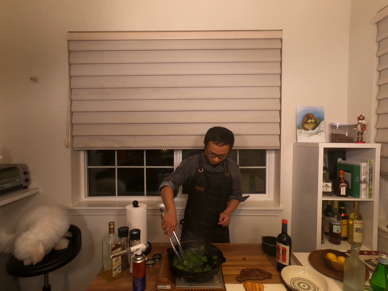
(a) Ground-Truth

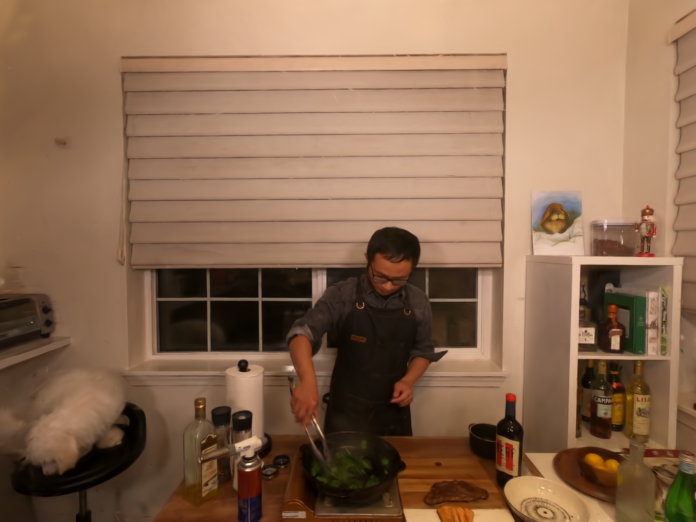
(b) TC3DGS Render

Figure 6: Qualitative Evaluation on the Neural 3D Video dataset. This figure shows a comparison between the ground truth and our reconstruction, demonstrating that our method achieves near-identical results (PSNR: 32.7) despite extreme compression.

Table 3: Ablation study on the proposed contributions. ‘M’, ‘Q’ and ‘I’ denote masking, quantization, interpolation, respectively. ‘#Gauss’ means the number of Gaussians.

Method \Dataset			Basketball				Cook Spinach
M	Q	I	PSNR	#Gauss	Storage	FPS	PSNR	#Gauss	Storage	FPS
Dynamic 3DGS			28.2	349K	2161 MB	582	33.1	294K	3370 MB	472
✓			28.1	189K	1087 MB	750	32.9	59 K	674 MB	583
✓	✓		27.9	189K	299 MB	750	32.8	59 K	194 MB	583
✓	✓	✓	27.9	189K	46 MB	750	32.7	59 K	53 MB	583

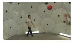
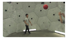
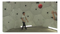
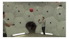
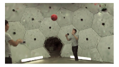
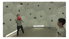
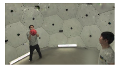
Dynamic 3DGS [26]	Pruned	Quantized + Pruned	Quantized + Pruned + KPI

Figure 7: Ablation study. Adding the different components of our method comes at virtually no cost in visual accuracy but at significantly decreased storage and rendering cost.

As shown in Table 1, our method achieves results comparable to Dynamic 3DGS [26], while utilizing, on average, 40 times less storage. Similarly, Table 2 presents the results of our method on the DyNeRF dataset, demonstrating competitive performance with a significantly smaller storage footprint. Furthermore, our approach delivers the fastest rendering speed.

On the Panoptic dataset, we failed to obtain reasonable results for the STG baseline [23], while 4D Gaussian [38] produce very distorted images, as shown in Figure 2. This dataset demonstrates the strengths of explicit methods such as Dynamic 3DGS [26] and ours. While Dynamic 3DGS [26] is able to model the complex motion and perform well on the Panoptic dataset, it is highly memory inefficient. In comparison, our model performs equally well while using much less storage.

4.4 Ablation Studies

We conduct an ablation study to evaluate the effectiveness of the individual components of our method. We report the results of this ablation in Table 3 on two scenes from the Panoptic dataset [18] and the Neural 3D Video dataset [22].

These results show the importance of each component of our method in reducing the storage size of the 3DGS [26]. In these experiments, our pruning strategy divides the number of Gaussians by 2 and by 5 folds for each scene. Then, sensitivity-aware quantization reduces the necessary storage space by 5, and keypoint interpolation by an additional 4 to 5 fold. Altogether, TC3DGS yields a compression ratio of 49 and 64, respectively. Most notably, this drastic size reduction comes at little to no cost in novel view synthesis, with an insignificant drop in PSNR of at most 0.4, which is barely perceptible.

5 Limitations

Our approach has certain limitations rooted in the nature of dynamic 3D Gaussian splatting (3DGS) and the constraints of compressing temporal data for dynamic scenes. First, unlike compression approaches for static 3DGS, we are limited in our ability to aggressively compress position parameters, as doing so would compromise temporal consistency and spatial accuracy in the dynamic setting. Additionally, as our method builds on Dynamic 3DGS, it inherits its inability to accurately reconstruct new objects that enter the scene after the initial frame. This restricts its use in scenarios requiring complete adaptability to scene changes. Nonetheless, our method excels at handling scenes with complex and fast motions, maintaining high fidelity and rendering efficiency despite these constraints.

6 Conclusion

We introduced Temporally Compressed 3D Gaussian Splatting (TC3DGS), a novel framework designed to achieve memory-efficient and high-speed reconstruction of dynamic scenes. Our method achieves up to 67x compression and up to three times faster rendering while retaining high fidelity in complex motion scenarios. Through selective temporal pruning and gradient-based quantization, TC3DGS minimizes memory usage with minimal impact on visual quality. While our method is effective, limitations remain in aggressively compressing position data and handling new objects that enter the scene mid-sequence. Future work will focus on bridging the gap between spatio-temporal methods and storage-efficient dynamic scene reconstruction, aiming to extend adaptability and further reduce storage requirements for complex, evolving environments.

Supplementary Material

7 Technicolor Dataset [34]

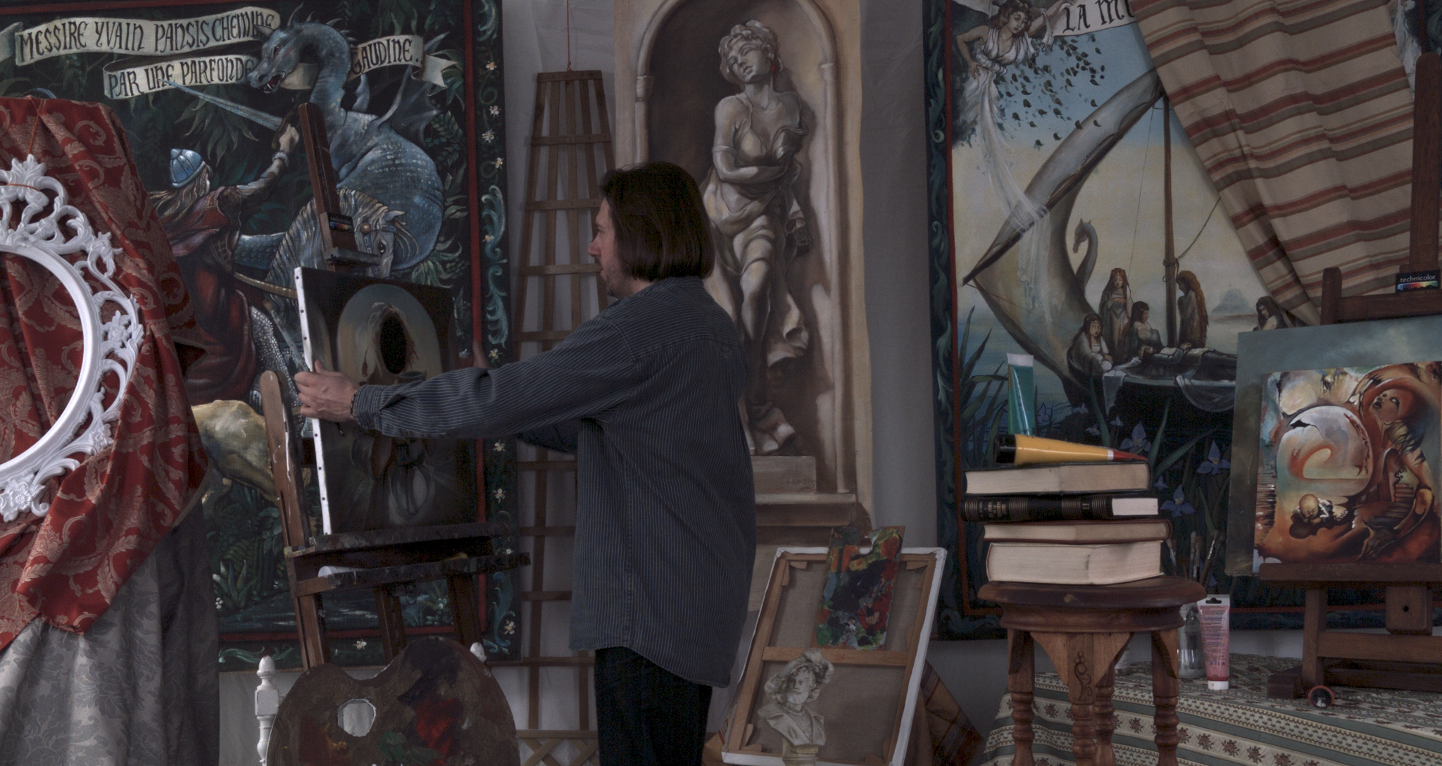
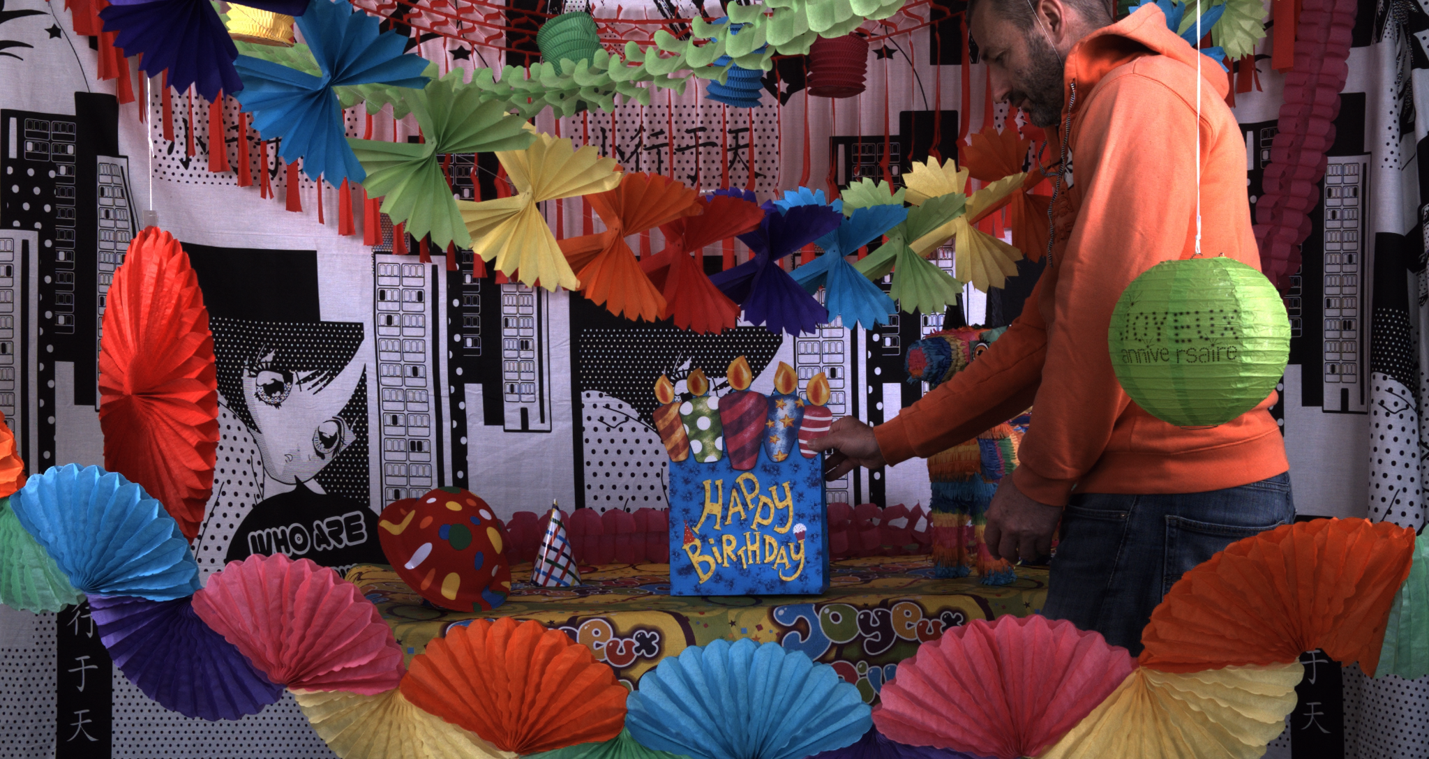
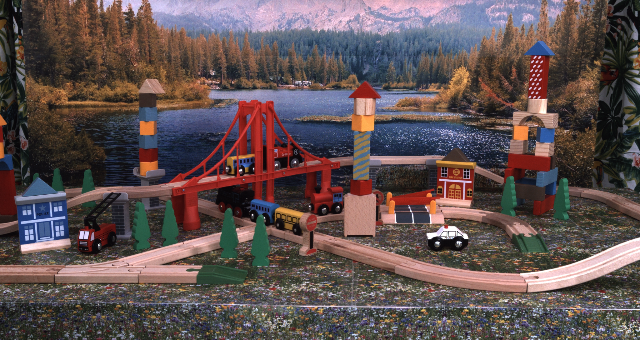
(a) Ground-Truth

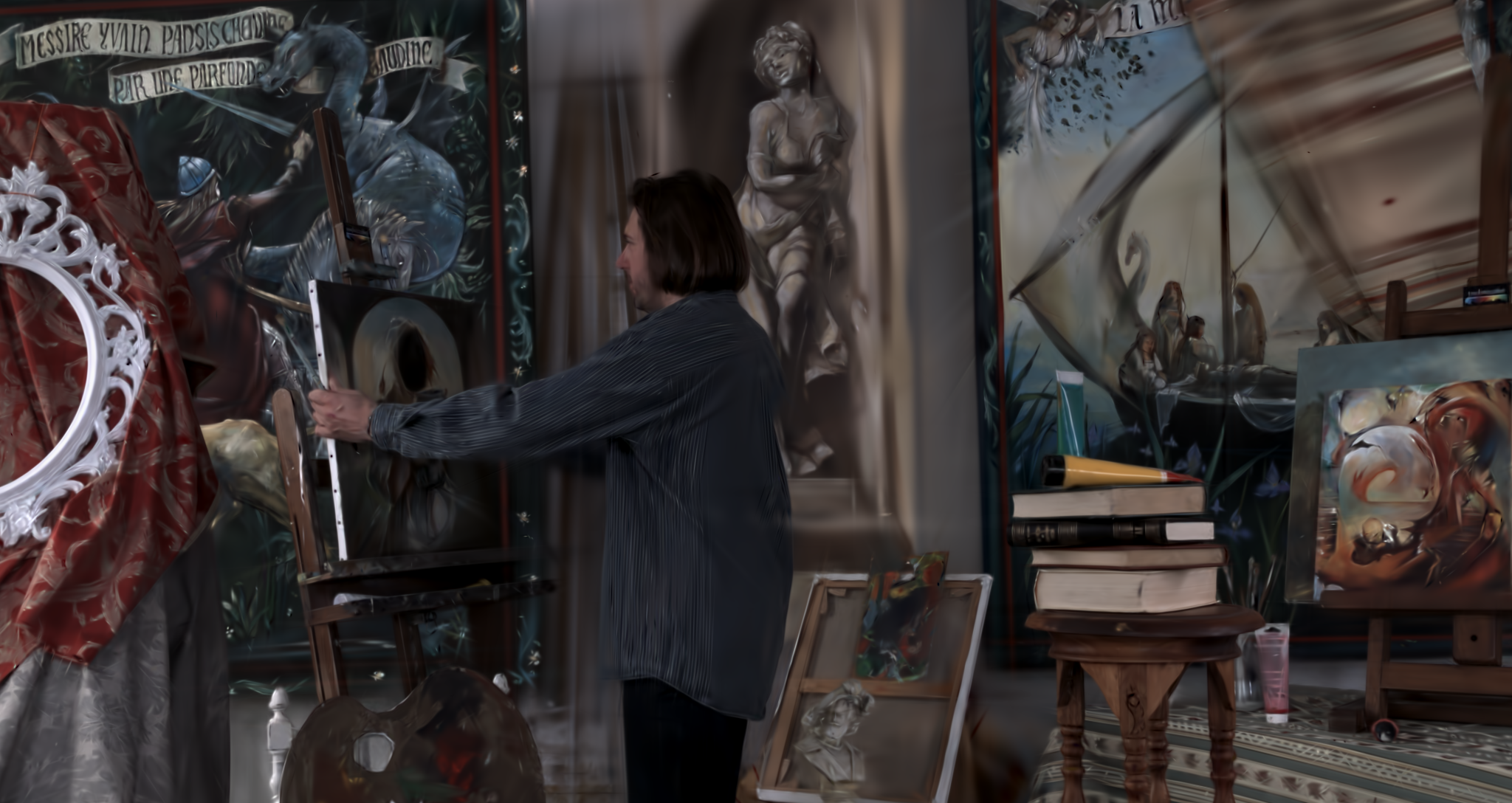
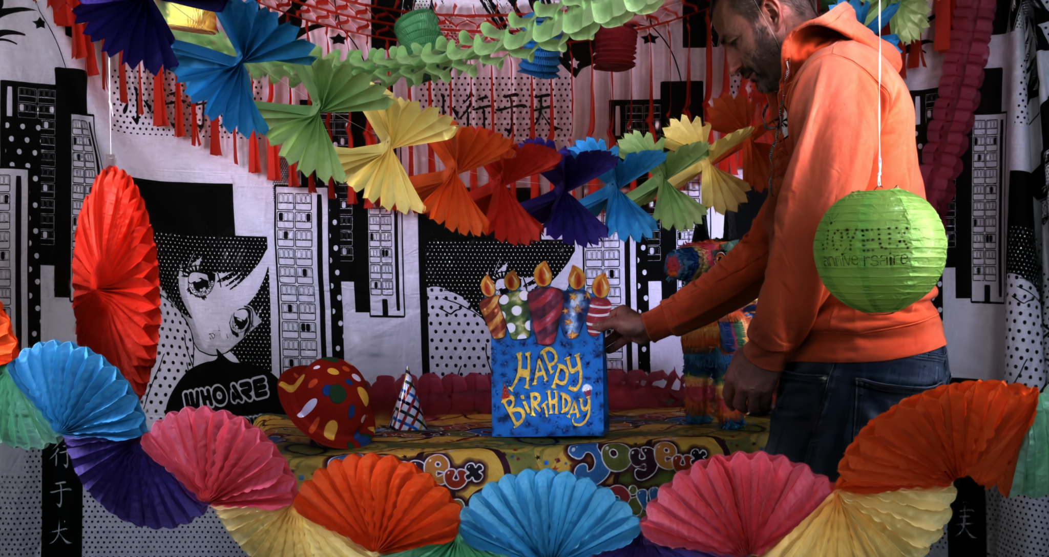
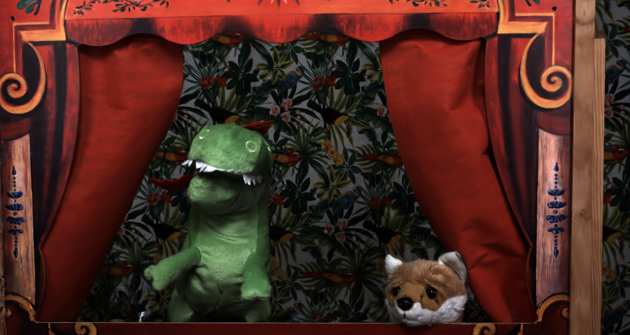
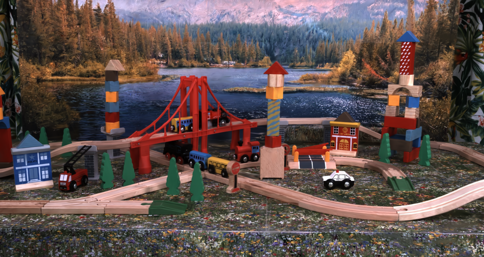
(b) TC3DGS Render

Figure 11: Qualitative Evaluation on the Technicolor dataset. This figure shows a comparison between the ground truth and our reconstruction, demonstrating that our method achieves near-identical results despite extreme compression.

To further demonstrate the effectiveness of our method, we evaluate our method on the Technicolor Dataset. The results in Table 4 show that our method provides competitive performance with a significantly smaller storage footprint. Figure 11 shows a comparison between the ground truth and our reconstruction, demonstrating that our method achieves near identical results.

Table 4: Per-Scene Results on the Technicolor Dataset. Our method achieves performance comparable to Dynamic3DGS [26] while significantly reducing the model size.

Method	Avg.	Birthday	Fabien	Painter	Theater	Train
PSNR$\uparrow$
STG [23]	$33.60$	$32.09$	$35.70$	$36.44$	$30.99$	$32.58$
D. 3DGS [26]	$32.12$	$30.82$	$33.62$	$34.73$	$31.12$	$30.67$
Ours	$31.9$	$30.33$	$33.15$	$34.62$	$31.01$	$30.57$
SSIM$\uparrow$
STG [23]	-	-	-	-	-	-
D. 3DGS [26]	$0.88$	$0.90$	$0.88$	$0.87$	$0.86$	$0.88$
Ours	$0.85$	$0.88$	$0.86$	$0.81$	$0.84$	$0.86$
LPIPS$\downarrow$
STG [23]	$0.08$	$0.04$	$0.11$	$0.10$	$0.13$	$0.04$
D. 3DGS [26]	$0.13$	$0.07$	$0.16$	$0.16$	$0.14$	$0.11$
Ours	$0.14$	$0.09$	$0.15$	$0.17$	$0.16$	$0.13$

Table 5: Per-scene quantitative comparisons on the Panoptic Sports Dataset [18].

Method	Avg.	Basket.	Juggle	Boxes	Softball	Tennis	Football
PSNR$\uparrow$
4DGaussians [38]	$27.2$	$26.68$	$27.47$	$27.02$	$27.44$	$27.31$	$27.39$
STG [23]	$20.45$	$21.60$	$19.93$	$20.65$	$19.44$	$20.82$	$20.23$
D. 3DGS [26]	28.70	28.22	29.48	29.46	28.43	28.11	28.49
Ours	$27.81$	$27.92$	$29.15$	$28.28$	$27.96$	$25.97$	$28.00$
SSIM$\uparrow$
4DGaussians [38]	0.91	$0.90$	0.92	0.91	0.92	0.92	0.92
STG [23]	$0.79$	$0.78$	$0.78$	$0.79$	$0.79$	$0.78$	$0.78$
D. 3DGS [26]	0.91	0.91	0.92	0.91	$0.91$	$0.91$	$0.91$
Ours	$0.89$	$0.89$	$0.90$	$0.89$	$0.89$	$0.89$	$0.89$
LPIPS$\downarrow$
4DGaussians [38]	$0.11$	0.14	0.10	0.10	0.10	0.11	0.10
STG [23]	0.10	0.14	0.10	0.10	0.10	0.11	0.10
D. 3DGS [26]	$0.17$	$0.18$	$0.15$	$0.17$	$0.19$	$0.18$	$0.17$
Ours	$0.20$	$0.20$	$0.19$	$0.19$	$0.20$	$0.20$	$0.20$
SIZE(MB)$\downarrow$
4DGaussians [38]	$63$	$66$	$59$	$63$	$57$	$72$	$65$
STG [23]	19	19	19	20	19	22	19
D. 3DGS [26]	$2008$	$2161$	$1935$	$2021$	$2021$	$1915$	$2000$
Ours	$49$	$46$	$32$	$44$	$41$	$48$	$34$

8 Detailed Results for Panoptic and Neural 3D Video Dataset

We present detailed results for the two datasets discussed in Sec. 4.1 of our paper, summarized in Table 5 and 8. These results include various metrics evaluated for each scene in both datasets, offering a granular view of performance. Additionally, we provide supplementary visualizations for the Neural 3D Video dataset, which further demonstrate the effectiveness of our method in capturing dynamic scenes with high fidelity. Finally, we present an ablation study over the main elements of our method in Figure 8.

9 Additional Experiments

We conducted several experiments to better understand hyperparameters of our method.

9.1 Masking and Mask Consistency

We vary the weight of the mask loss $\lambda_{\text{mask}}$ and the masking consistency loss $\lambda_{\text{mask-cons}}$ on the first 50 frames of the Basketball scene from the Panoptic Sports dataset. The results, shown in Table 6, indicate that increasing the weight of these parameters leads to greater pruning of Gaussians but results in reduced image quality. We found $\lambda_{\text{mask}}=\lambda_{\text{mask-cons}}=0.01$ to be an effective balance between maintaining image quality and minimizing model size.

(a) SSIM $\uparrow$

	Mask Consistency Loss
Mask Loss	0	0.01	0.05	0.1
0.005	0.9087	0.9105	0.9109	0.9068
0.01	0.9126	0.9140	0.9113	0.9092
0.05	0.9036	0.9006	0.8986	0.8970
0.1	0.8938	0.8956	0.8949	0.8972

(b) PSNR $\uparrow$

	Mask Consistency Loss
Mask Loss	0	0.01	0.05	0.1
0.005	28.0	27.8	28.2	26.8
0.01	28.1	28.3	26.8	26.9
0.05	27.2	26.6	26.0	26.0
0.1	27.1	27.4	26.6	26.7

(c) LPIPS $\downarrow$

	Mask Consistency Loss
Mask Loss	0	0.01	0.05	0.1
0.005	0.1797	0.1769	0.1781	0.1815
0.01	0.1746	0.1761	0.1748	0.1829
0.05	0.2046	0.2090	0.2139	0.2172
0.1	0.2345	0.2294	0.2344	0.2335

(d) Number of Gaussians $\downarrow$

	Mask Consistency Loss
Mask Loss	0	0.01	0.05	0.1
0.005	208403	155720	143112	140897
0.01	153757	112909	98017	93568
0.05	49770	47110	29629	26154
0.1	28972	31067	19472	15656

Table 6: Impact of Mask Loss and Mask Consistency Loss. Increasing the weight of these masks leads to more aggressive pruning of Gaussians, but at the cost of rendering quality. Setting $\lambda_{mask}=0.01$ and $\lambda_{mask-cons}=0.01$ provides a good trade-off between quality and storage efficiency.

9.2 Quantization

We ran experiments with sensitivity-aware quantization with different bit-ranges by varying $b_{\text{min}}$ and $b_{\text{max}}$ as well as using uniform bitwidth for all paramaters. We shown in the Table 7 that using adaptive bitwidth, the average bitwidth is lower than uniform quantization at 8 bits while image quality is similar. Whereas, compared to uniform quantization using lower bitwidth, our average bitwidth is slightly higher while image quality is improved considerably.

Bit-precision	PSNR	SSIM	LPIPS	Compression
uniform 4 bit	25.1	0.81	0.32	8x
uniform 5 bit	25.8	0.84	0.28	6.4x
uniform 6 bit	26.1	0.86	0.26	5.3x
uniform 8 bit	28.1	0.90	0.20	4x
Ours [5,8]	28.0	0.90	0.20	5.6x
Ours [4,8]	27.9	0.90	0.20	6.3x
Ours [3,8]	26.2	0.84	0.28	7.3x

Table 7: Comparison of Sensitivity-Aware and Uniform Bit Quantization. Our sensitivity-aware [4,8]-bit quantization achieves PSNR comparable to 8-bit precision while providing compression similar to uniform 5-bit quantization.

9.3 Keypoint Interpolation

We experimented with varying the hyperparameters for keypoint interpolation, specifically the maximum number of keypoints, $max_{kp}$. As shown in Figure 9, increasing $max_{kp}$ reduces compression error and improves image quality. Conversely, increasing $\tau$ allows for greater error tolerance, leading to a decrease in image quality.

The experiments summarized in Figure 9 were conducted on 150 frames of the Basketball scene with masking parameters set to $\lambda_{\text{mask}}=\lambda_{\text{mask-cons}}=0.01$ and fixed $tau=1\times e^{-6}$. We observed that overly relaxing $\tau$ leads to underfitted keypoints, resulting in compromised rendering quality. On the other hand, increasing $max_{kp}$ beyond a certain threshold results in diminishing returns, where interpolation error continues to decrease, but the improvement in image quality becomes marginal.

Additionally, Figure 10 illustrates that only the color parameters saturate the maximum keypoints, whereas positions and rotations can be adequately approximated with fewer keypoints.

We selected the hyperparameters to strike a balance between rendering quality and storage efficiency. For the Panoptic Sports dataset, we used $max_{kp}=30$ and $\tau=1\times 10^{-5}$. For the Neural 3D Video dataset, which consists of 300-frame sequences, we increased $max_{kp}$ to 60 to accommodate the longer sequence length. In the case of the Technicolor dataset, despite its long sequences, we matched the experimental setup by using 50 timesteps per scene and reduced $max_{kp}$ to 15.

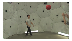
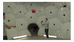
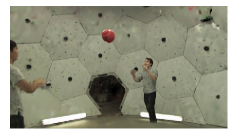
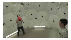
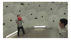
Dynamic 3DGS [26]	Pruned	Quantized + Pruned	Quantized + Pruned + KPI

Figure 8: Ablation Study on Panoptic Sports Dataset

Table 8: Per-scene quantitative comparisons on the Neural 3D Video Dataset [22]. Some methods only report part of the scenes. ¹ only includes the Flame Salmon scene. ² excludes the Coffee Martini scene. “-” denotes results that are unavailable in prior work.

Method	Avg.	Coffee Martini	Cook Spinach	Cut Roasted Beef	Flame Salmon	Flame Steak	Sear Steak
PSNR$\uparrow$
Neural Volumes [25] 1	$22.80$	-	-	-	$22.80$	-	-
LLFF [27] 1	$23.24$	-	-	-	$23.24$	-	-
DyNeRF [22] 1	$29.58$	-	-	-	$29.58$	-	-
HexPlane [3] 2	$31.71$	-	$32.04$	$32.55$	$29.47$	$32.08$	$32.39$
NeRFPlayer [36]	$30.69$	31.53	$30.56$	$29.35$	$31.65$	$31.93$	$29.13$
HyperReel [1]	$31.10$	$28.37$	$32.30$	$32.92$	$28.26$	$32.20$	$32.57$
K-Planes [16]	$31.63$	$29.99$	$32.60$	$31.82$	$30.44$	$32.38$	$32.52$
MixVoxels-L [37]	$31.34$	$29.63$	$32.25$	$32.40$	$29.81$	$31.83$	$32.10$
MixVoxels-X [37]	$31.73$	$30.39$	$32.31$	$32.63$	30.60	$32.10$	$32.33$
4D Gaussians [38]	$30.67$	$27.34$	$32.46$	$32.90$	$29.20$	$32.51$	$32.49$
Dynamic 3DGS [26]	$30.97$	$27.32$	$32.97$	$31.75$	$27.26$	$33.24$	$33.68$
STG [23]	32.05	$28.61$	33.18	$33.52$	$29.48$	33.64	33.89
Ours	$30.58$	$27.42$	$31.92$	33.61	$27.12$	$32.48$	$33.04$
LPIPS$\downarrow$
Neural Volumes [25] 1	$0.295$	-	-	-	$0.295$	-	-
LLFF [27] 1	$0.235$	-	-	-	$0.235$	-	-
DyNeRF [22] 1	$0.083$	-	-	-	$0.083$	-	-
HexPlane [3] 2	$0.075$	-	$0.082$	$0.080$	$0.078$	$0.066$	$0.070$
NeRFPlayer [36]	$0.111$	$0.085$	$0.113$	$0.144$	$0.098$	$0.088$	$0.138$
HyperReel [1]	$0.096$	$0.127$	$0.089$	$0.084$	$0.136$	$0.078$	$0.077$
MixVoxels-L [37]	$0.096$	$0.106$	$0.099$	$0.088$	$0.116$	$0.088$	$0.080$
MixVoxels-X [37]	$0.064$	$0.081$	$0.062$	$0.057$	$0.078$	$0.051$	$0.053$
Dynamic 3DGS [26]	$0.082$	$0.122$	$0.077$	$0.087$	$0.09$	$0.072$	$0.068$
STG [23]	0.044	0.069	0.037	0.036	0.063	0.029	0.030
Ours	$0.089$	$0.129$	$0.081$	$0.088$	$0.094$	$0.075$	$0.071$

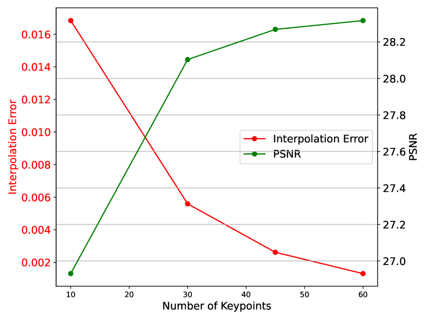
(a) Interpolation Error and PSNR vs Maximum Keypoints

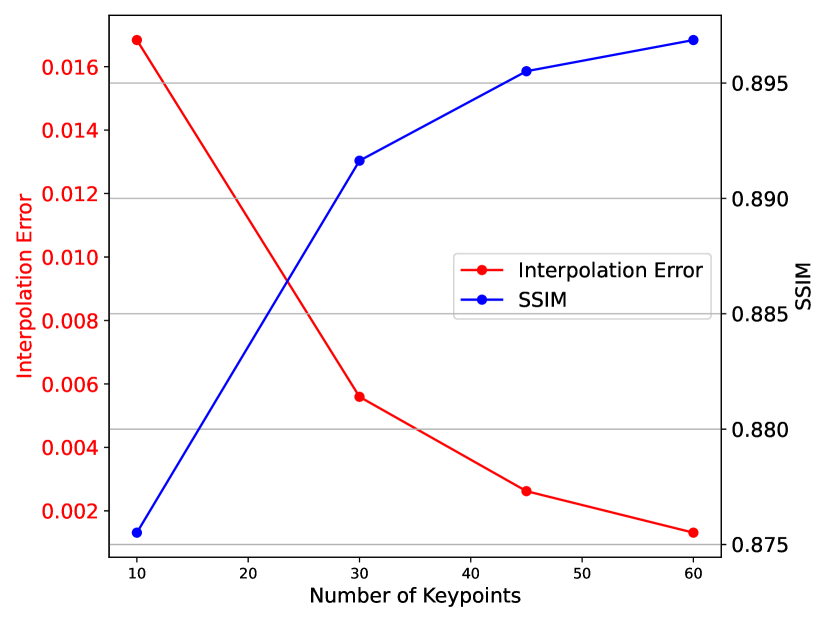
(b) Interpolation Error and SSIM vs Maximum Keypoints

Figure 9: Impact of increasing Maximum Keypoints The figure illustrates the trend of interpolation error and PSNR/SSIM as we increase $max_{kp}$. It highlights that the rate of change in interpolation error and PSNR/SSIM diminishes as we increase $max_{kp}$

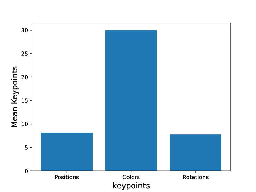
(a) Mean number of Keypoints

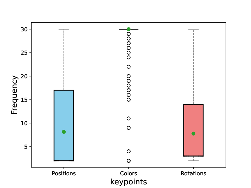
(b) Distribution of Keypoints

Figure 10: Distribution of Keypoints Across Different Parameters. The figure illustrates the mean number of keypoints for Gaussian parameters. It highlights that only color parameters reach $max_{kp}$ saturation, while positions and rotations can be effectively estimated with fewer keypoints.

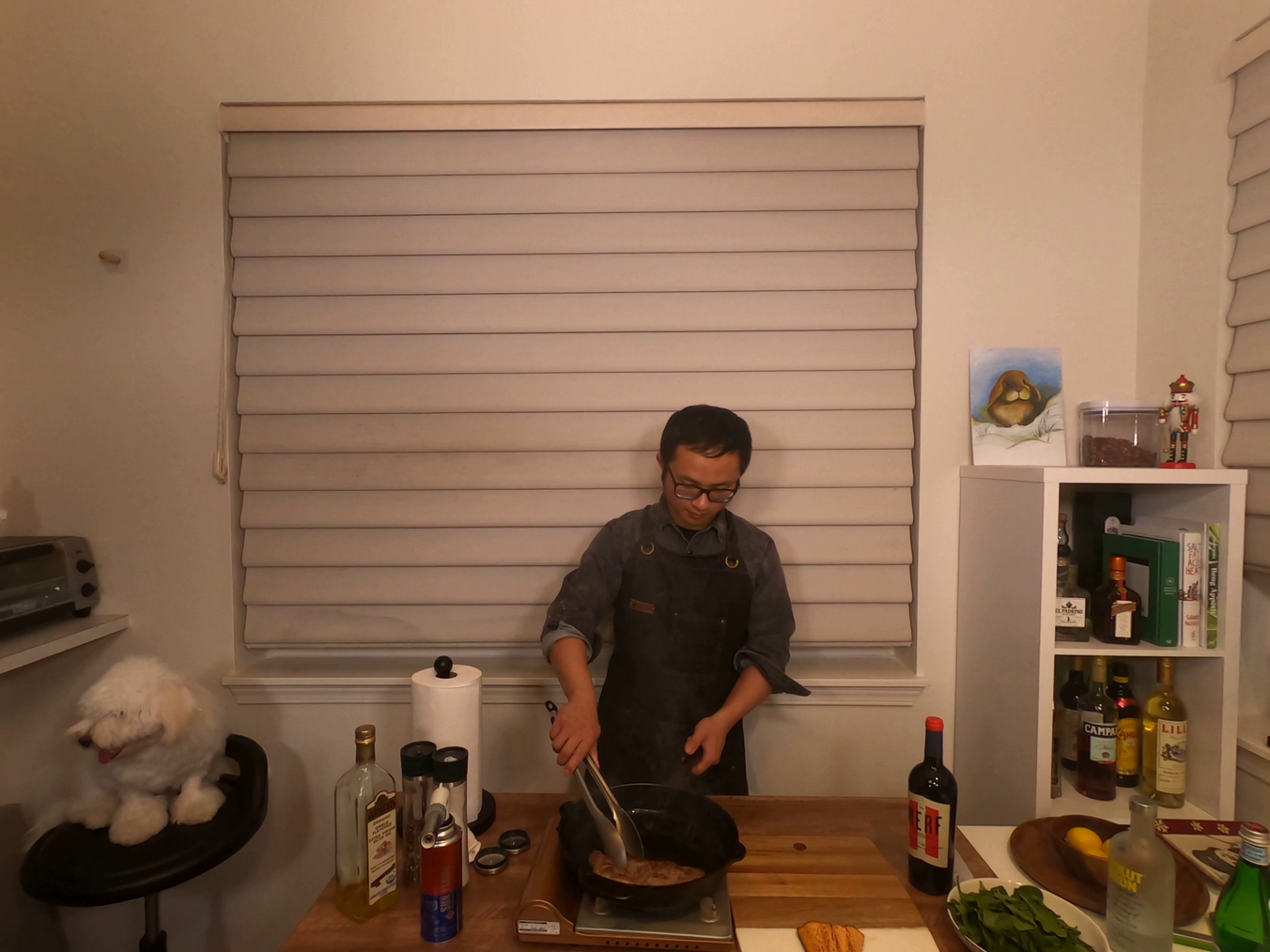
(a) Ground-Truth

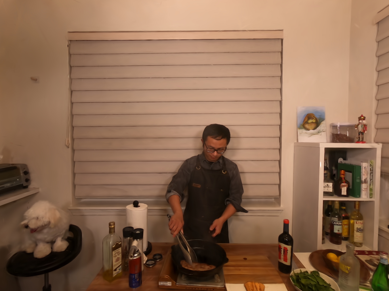
(b) TC3DGS Render

Figure 12: Qualitative Evaluation on the Neural 3D Video Dataset. This figure shows a comparison between the ground truth and our reconstruction, demonstrating that our method achieves near-identical results despite extreme compression. Top: Cook Spinach, Bottom: Sear Steak

References

- Attal et al. [2023] Benjamin Attal, Jia-Bin Huang, Christian Richardt, Michael Zollhoefer, Johannes Kopf, Matthew O’Toole, and Changil Kim. HyperReel: High-Fidelity 6-DoF Video with Ray-Conditioned Sampling. In CVPR, 2023.
- Bae et al. [2024] Jeongmin Bae, Seoha Kim, Youngsik Yun, Hahyun Lee, Gun Bang, and Youngjung Uh. Per-Gaussian Embedding-Based Deformation for Deformable 3D Gaussian Splatting. In ECCV, 2024.
- Cao and Johnson [2023] Ang Cao and Justin Johnson. HexPlane: A Fast Representation for Dynamic Scenes. 2023.
- Chen et al. [2022] Anpei Chen, Zexiang Xu, Andreas Geiger, Jingyi Yu, and Hao Su. Tensorf: Tensorial radiance fields. In ECCV, 2022.
- Chen et al. [2025] Yihang Chen, Qianyi Wu, Weiyao Lin, Mehrtash Harandi, and Jianfei Cai. Hac: Hash-grid assisted context for 3d gaussian splatting compression. In ECCV, 2025.
- Das et al. [2024] Devikalyan Das, Christopher Wewer, Raza Yunus, Eddy Ilg, and Jan Eric Lenssen. Neural parametric gaussians for monocular non-rigid object reconstruction. In CVPR, 2024.
- DOUGLAS and PEUCKER [1973] DAVID H DOUGLAS and THOMAS K PEUCKER. ALGORITHMS FOR THE REDUCTION OF THE NUMBER OF POINTS REQUIRED TO REPRESENT A DIGITIZED LINE OR ITS CARICATURE. Cartographica, 10(2):112–122, 1973.
- Duan et al. [2024a] Yuanxing Duan, Fangyin Wei, Qiyu Dai, Yuhang He, Wenzheng Chen, and Baoquan Chen. 4d-rotor gaussian splatting: towards efficient novel view synthesis for dynamic scenes. In ACM SIGGRAPH, 2024a.
- Duan et al. [2024b] Yuanxing Duan, Fangyin Wei, Qiyu Dai, Yuhang He, Wenzheng Chen, and Baoquan Chen. 4D-Rotor Gaussian Splatting: Towards Efficient Novel View Synthesis for Dynamic Scenes. In SIGGRAPH, 2024b.
- Esser et al. [2020] Steven K. Esser, Jeffrey L. McKinstry, Deepika Bablani, Rathinakumar Appuswamy, and Dharmendra S. Modha. LEARNED STEP SIZE QUANTIZATION. In ICLR, 2020.
- Fan et al. [2024] Zhiwen Fan, Kevin Wang, Kairun Wen, Zehao Zhu, Dejia Xu, and Zhangyang Wang. LightGaussian: Unbounded 3D Gaussian Compression with 15x Reduction and 200+ FPS. 2024.
- Fang and Wang [2024] Guangchi Fang and Bing Wang. Mini-Splatting: Representing Scenes with a Constrained Number of Gaussians. In ECCV, 2024.
- Fang et al. [2022] Jiemin Fang, Taoran Yi, Xinggang Wang, Lingxi Xie, Xiaopeng Zhang, Wenyu Liu, Matthias Nießner, and Qi Tian. Fast Dynamic Radiance Fields with Time-Aware Neural Voxels. In SIGGRAPH Asia, 2022.
- Franke et al. [2024] Linus Franke, Darius Rückert, Laura Fink, and Marc Stamminger. TRIPS: Trilinear Point Splatting for Real-Time Radiance Field Rendering. Computer Graphics Forum, 2024.
- Fridovich-Keil et al. [2022] Sara Fridovich-Keil, Alex Yu, Matthew Tancik, Qinhong Chen, Benjamin Recht, and Angjoo Kanazawa. Plenoxels: Radiance fields without neural networks. In CVPR, 2022.
- Fridovich-Keil et al. [2023] Sara Fridovich-Keil, Giacomo Meanti, Frederik Rahbæk Warburg, Benjamin Recht, and Angjoo Kanazawa. K-Planes: Explicit Radiance Fields in Space, Time, and Appearance. In CVPR, 2023.
- Girish et al. [2024] Sharath Girish, Kamal Gupta, and Abhinav Shrivastava. EAGLES: Efficient Accelerated 3D Gaussians with Lightweight EncodingS. In ECCV, 2024.
- Joo et al. [2019] Hanbyul Joo, Tomas Simon, Xulong Li, Hao Liu, Lei Tan, Lin Gui, Sean Banerjee, Timothy Godisart, Bart Nabbe, Iain Matthews, Takeo Kanade, Shohei Nobuhara, and Yaser Sheikh. Panoptic Studio: A Massively Multiview System for Social Interaction Capture. TPAMI, 2019.
- Katsumata et al. [2025] Kai Katsumata, Duc Minh Vo, and Hideki Nakayama. A compact dynamic 3d gaussian representation for real-time dynamic view synthesis. In ECCV, 2025.
- Kerbl et al. [2023] Bernhard Kerbl, Georgios Kopanas, Thomas Leimkühler, and George Drettakis. 3D Gaussian Splatting for Real-Time Radiance Field Rendering. ACM TOG, 2023.
- Lee et al. [2024] Joo Chan Lee, Daniel Rho, Xiangyu Sun, Jong Hwan Ko, and Eunbyung Park. Compact 3d gaussian representation for radiance field. In CVPR, 2024.
- Li et al. [2022] Tianye Li, Mira Slavcheva, Michael Zollhoefer, Simon Green, Christoph Lassner, Changil Kim, Tanner Schmidt, Steven Lovegrove, Michael Goesele, Richard Newcombe, and Zhaoyang Lv. Neural 3D Video Synthesis from Multi-view Video. arXiv preprint arXiv:2103.02597, 2022.
- Li et al. [2024] Zhan Li, Zhang Chen, Zhong Li, and Yi Xu. Spacetime gaussian feature splatting for real-time dynamic view synthesis. In CVPR, 2024.
- Liu et al. [2023] Yu-Lun Liu, Chen Gao, Andreas Meuleman, Hung-Yu Tseng, Ayush Saraf, Changil Kim, Yung-Yu Chuang, Johannes Kopf, and Jia-Bin Huang. Robust dynamic radiance fields. In CVPR, 2023.
- Lombardi et al. [2019] Stephen Lombardi, Tomas Simon, Jason Saragih, Gabriel Schwartz, Andreas Lehrmann, and Yaser Sheikh. Neural Volumes: Learning Dynamic Renderable Volumes from Images. ACM Transactions on Graphics (TOG), 2019.
- Luiten et al. [2024] Jonathon Luiten, Georgios Kopanas, Bastian Leibe, and Deva Ramanan. Dynamic 3D Gaussians: Tracking by Persistent Dynamic View Synthesis. In 3DV, 2024.
- Mildenhall et al. [2019] Ben Mildenhall, Pratul P. Srinivasan, Rodrigo Ortiz-Cayon, Nima Khademi Kalantari, Ravi Ramamoorthi, Ren Ng, and Abhishek Kar. Local Light Field Fusion: Practical View Synthesis with Prescriptive Sampling Guidelines. ACM Transactions on Graphics (TOG), 2019.
- Mildenhall et al. [2021] Ben Mildenhall, Pratul P Srinivasan, Matthew Tancik, Jonathan T Barron, Ravi Ramamoorthi, and Ren Ng. Nerf: Representing scenes as neural radiance fields for view synthesis. Communications of the ACM, 2021.
- Morgenstern et al. [2024] Wieland Morgenstern, Florian Barthel, Anna Hilsmann, and Peter Eisert. Compact 3D Scene Representation via Self-Organizing Gaussian Grids. In ECCV, 2024.
- Müller et al. [2022] Thomas Müller, Alex Evans, Christoph Schied, and Alexander Keller. Instant neural graphics primitives with a multiresolution hash encoding. ACM TOG, 2022.
- Navaneet et al. [2024] KL Navaneet, Kossar Pourahmadi Meibodi, Soroush Abbasi Koohpayegani, and Hamed Pirsiavash. CompGS: Smaller and faster gaussian splatting with vector quantization. In ECCV, 2024.
- Niedermayr et al. [2024] Simon Niedermayr, Josef Stumpfegger, and Rüdiger Westermann. Compressed 3D Gaussian Splatting for Accelerated Novel View Synthesis. In CVPR, 2024.
- Pumarola et al. [2021] Albert Pumarola, Enric Corona, Gerard Pons-Moll, and Francesc Moreno-Noguer. D-nerf: Neural radiance fields for dynamic scenes. In CVPR, 2021.
- Sabater et al. [2017] Neus Sabater, Guillaume Boisson, Benoit Vandame, Paul Kerbiriou, Frederic Babon, Matthieu Hog, Tristan Langlois, Remy Gendrot, Olivier Bureller, Arno Schubert, and Valerie Allie. Dataset and Pipeline for Multi-View Light-Field Video. In CVPR, 2017.
- Shao et al. [2023] Ruizhi Shao, Zerong Zheng, Hanzhang Tu, Boning Liu, Hongwen Zhang, and Yebin Liu. Tensor4D: Efficient Neural 4D Decomposition for High-fidelity Dynamic Reconstruction and Rendering. In CVPR, 2023.
- Song et al. [2023] Liangchen Song, Anpei Chen, Zhong Li, Zhang Chen, Lele Chen, Junsong Yuan, Yi Xu, and Andreas Geiger. Nerfplayer: A streamable dynamic scene representation with decomposed neural radiance fields. IEEE Transactions on Visualization and Computer Graphics, 2023.
- Wang et al. [2023] Feng Wang, Sinan Tan, Xinghang Li, Zeyue Tian, Yafei Song, and Huaping Liu. Mixed Neural Voxels for Fast Multi-view Video Synthesis. In ICCV, 2023.
- Wu et al. [2024a] Guanjun Wu, Taoran Yi, Jiemin Fang, Lingxi Xie, Xiaopeng Zhang, Wei Wei, Wenyu Liu, Qi Tian, and Xinggang Wang. 4D Gaussian Splatting for Real-Time Dynamic Scene Rendering. In CVPR, 2024a.
- Wu et al. [2024b] Guanjun Wu, Taoran Yi, Jiemin Fang, Lingxi Xie, Xiaopeng Zhang, Wei Wei, Wenyu Liu, Qi Tian, and Xinggang Wang. 4d gaussian splatting for real-time dynamic scene rendering. In CVPR, 2024b.
- Yang et al. [2024a] Ziyi Yang, Xinyu Gao, Wen Zhou, Shaohui Jiao, Yuqing Zhang, and Xiaogang Jin. Deformable 3d gaussians for high-fidelity monocular dynamic scene reconstruction. In CVPR, 2024a.
- Yang et al. [2024b] Zeyu Yang, Hongye Yang, Zijie Pan, and Li Zhang. Real-time Photorealistic Dynamic Scene Representation and Rendering with 4D Gaussian Splatting. In ICLR, 2024b.
- Zhang et al. [2024a] Zhaoliang Zhang, Tianchen Song, Yongjae Lee, Li Yang, Cheng Peng, Rama Chellappa, and Deliang Fan. LP-3DGS: Learning to Prune 3D Gaussian Splatting. arXiv preprint arXiv:2405.18784, 2024a.
- Zhang et al. [2024b] Zhi Zhang, Qizhe Zhang, Zijun Gao, Renrui Zhang, Ekaterina Shutova, Shiji Zhou, and Shanghang Zhang. Gradient-based Parameter Selection for Efficient Fine-Tuning. In CVPR, 2024b.