Kinematic evidence of magnetospheric accretion for Herbig Ae stars with JWST NIRSpec.

Abstract

Context. Hydrogen emission lines have been used to estimate the mass accretion rate of pre-main-sequence stars for over $25$ years. Despite the clear correlation between the accretion luminosity of a star and hydrogen line luminosities, the physical origin of these lines is still unclear, with magnetospheric accretion and magneto-centrifugal winds as the two most often invoked mechanisms.

Aims. Using a combination of HST photometry and new JWST NIRSpec spectra in the range $1.66-3.2\mu m$, we have analysed the spectral energy distributions (SED) and emission line spectra of five sources in order to determine their underlying photospheric properties, and to attempt to reveal the physical origin of their hydrogen emission lines. These sources reside in NGC 3603, a Galactic massive star forming region.

Methods. We have fitted the SED of the five sources employing a Markov Chain Monte Carlo exploration to estimate $T_{eff}$, $R_{*}$, $M_{*}$ and $A(V)$ for each source. We have performed a kinematic analysis across three spectral series of hydrogen lines, Paschen, Brackett, and Pfund, totalling $\geq 15$ lines. The full width at half maximum (FWHM) and optical depth of the spectrally resolved lines have been studied in order to constrain the emission origin.

Results. The five sources all have SEDs consistent with young intermediate-mass stars. We have classified three of these sources as Herbig Ae type stars based on their effective temperature. Their hydrogen lines show broad profiles with FWHMs $\geq 200$ km s^-1. Hydrogen lines with high upper energy levels $n_{up}$ tend to be significantly broader than lines with lower $n_{up}$. The optical depth of the emission lines is also highest for the high velocity component of each line, becoming optically thin in the low velocity component.

Conclusions. The highest excitation lines have the largest FWHM for a given series. The highest velocity component of the lines is also the most optically thick. This is consistent with emission from a magnetospheric accretion flow, and cannot be explained as originating in a magneto-centrifugal wind, or other line emission mechanisms thought to be present in protoplanetary disks.

1 Introduction

Protoplanetary disks around young stars are the site of numerous highly studied astronomical phenomena, including magnetospheric accretion flows, accelerating disk winds powered by magneto-centrifugal forces, and, as the name suggests, are the formation site of planets. Understanding the evolution of protoplanetary disks is crucial in both the context of star formation and planet formation. A fundamental push and pull that regulates the lifetime of protoplanetary disks is the balance between mass-loss through winds and mass accretion onto the central star.
Accretion rates of stars were originally measured by fitting shock models to the near-ultraviolet (NUV) spectra of young low mass stars, known as Classical T Tauri Stars (CTTS) (Gullbring et al. 1998). The physical picture assumed here is centred around a magnetically driven accretion paradigm, in which the star’s strong magnetic field pushes against and truncates the protoplanetary disk out to a few stellar radii (e.g. Hartmann et al. 2016). Material at the disk’s surface is channelled along magnetic field lines from the disk to the central star. During its near free-fall towards the star, the supersonic material shocks the stellar surface, and releases its gravitational potential energy as radiation. Initially this is primarily in the form of X-rays, which are quickly absorbed by the stellar surface and re-radiated at longer wavelengths, in the NUV and blue-optical. This additional source of NUV light on top of the intrinsic photospheric contribution can be observed and measured, and from this so-called “accretion luminosity” the mass accretion rate can be determined. This is the only direct method of measuring the accretion luminosity, and while it unambiguously probes the accretion shock, the reliance on NUV wavelengths makes this impractical for sources that are deeply embedded or located at great distances, due to high levels of extinction.
An invaluable calibration was discovered by Muzerolle et al. (1998b), who showed that the line luminosity of the relatively bright near-infrared (NIR) hydrogen line $Br_{7}$ scales tightly with the accretion luminosity for a sample of $19$ CTTS. With extinction being $\geq 10$ times lower in the NIR compared to the NUV and without the need for shock modelling, this line luminosity calibration opened the floodgates for the efficient and straightforward estimate of accretion rates for large samples of sources. These calibrations have since been updated and expanded, most notably by Herczeg & Hillenbrand (2008); Alcalá et al. (2014, 2017). We also showed in an earlier work that these calibrations could be extended towards the brightest NIR line - $Pa_{\alpha}$ (Rogers et al. 2024a), making estimating the accretion rate highly accessible in the era of JWST for extremely distant and embedded sources.
All of this work relies on the assumption that accretion is driven magnetically. First theorised by Koenigl (1991) and unambiguously confirmed observationally by Bouvier et al. (2007) for CTTS, the magnetospheric accretion paradigm for Herbig AeBe stars has not reached the same consensus. Unlike CTTS (spectral types M through G), stars of spectral type A and earlier are not expected to possess a convective envelope, which is thought the be the source of the strong and ordered magnetic fields present around CTTS (e.g. Kageyama & Sato 1997; Johns-Krull 2007). Despite lingering questions over their origin, magnetic fields have been measured towards dozens of Herbig AeBe stars, albeit with significantly lower field strengths compared to CTTS (Mendigutía 2020). Other spectroscopic signatures of infalling matter are also seen towards Herbig AeBe stars, such as red-shifted absorption profiles in He I and H I lines (Cauley & Johns-Krull 2015), though they are less prevalent compared to the occurrence rate in CTTS. In general, magnetospheres, if present, are expected to be smaller in Herbig Ae stars compared to CTTS, and may be entirely absent for early Be stars (Wichittanakom et al. 2020; Vioque et al. 2022).
Disk winds are ubiquitous around young stars. Powerful collimated jets and outflows have been spatially resolved for many nearby sources, with large scale jets being the defining physical feature of the class of objects known as Herbig-Haro objects (Reipurth & Bally 2001). The exact launching mechanism of these winds is still under debate, although there is a growing consensus that these outflows are the result of a magneto-centrifugal wind (e.g. Tabone et al. 2022), first theorised by Blandford & Payne (1982). These winds are expected to be crucial in the removal of angular momentum from the disk, ultimately facilitating accretion by ejecting material, causing outer disk material to migrate inwards (conserving angular momentum in the process), and replenishing the inner gas disk where accretion takes place (Frank et al. 2014).
Thus, there is no doubt that both winds and accretion give rise to hydrogen emission lines, but there is not yet a consensus on which of the two processes dominates the hydrogen line emission for a given stellar mass and stage of evolution. Using the JWST NIRSpec Micro-Shutter Assembly (MSA), we have obtained 100 stellar spectra including a number of young intermediate mass stars and Herbig Ae stars from $1.66-3.2\mu m$ in high resolution mode R $\sim$ 4000 (see section 6.1 for our discussion of the point source resolving power of NIRSpec), with the filter and grating combination F170LP/G235H. These stars all reside in the giant Galactic star forming region NGC 3603, located $7.2\pm 0.1$ kpc away (Drew et al. 2019). We present five of these sources here, which all show rich emission line spectra, featuring large, unbroken sections of the Brackett and Pfund hydrogen series, as well as the strong $Pa_{\alpha}$ line. We have performed a kinematic analysis on the hydrogen lines for each source in order to constrain the physical origin of these lines.
In section  2 we discuss the target selection. In section  3, the data reduction and post-processing steps are explained. In section 4, we describe our methods for fitting and measuring the emission lines and the spectra are displayed. In section  5, we present the SED fitting of our sources. In section  6, the kinematic analysis is presented. In section  7, we interpret our analysis and suggest a physical origin for the emission lines. We also address alternative emission line mechanisms outside of magnetic accretion and winds. In section  8 we summarise our findings.

2 Observations and target selection

The target selection procedure has already been described in Rogers et al. (2024a) and we summarise it briefly here. The spectra were obtained as part of a NIRSpec Guaranteed Time Observations (GTO) programme (ID=1225, PI G. De Marchi). For each source, we opened three neighbouring micro-shutters in a column of the MSA, forming a “mini-slit”. We placed the source in the central shutter, with the upper and lower micro-shutters observing the nebula. We employed a nodding pattern, nodding the telescope three times such that the source moved from the central shutter, to the upper shutter and finally the lower shutter. This pattern enabled the observation of additional nebular regions as new regions came into view with each nod. It also provided us with three spectra for each source, which could then be averaged together.

3 Data reduction

3.1 NIPS

The observations were largely reduced with the ESA Instrument Team’s pipeline known as the NIRSpec Instrument Pipeline Software (NIPS) (Alves de Oliveira et al. 2018). Additional reduction steps were also written specifically for these observations which are briefly discussed. NIPS is a framework for spectral extraction of NIRSpec data from the count-rate maps, performing all major reduction steps from dark current and bias subtraction to flat fielding, wavelength and flux calibration, background subtraction and extraction, with the final product being the 1D extracted spectrum.
One of the final steps before extraction is the rectification of the spectrum. The dispersed NIRSpec spectra are curved along the detector. Rectification is performed in order to “straighten” the spectrum. By doing this, the spectrum is resampled onto a uniform wavelength grid (each wavelength bin $\Delta\lambda$ is the same for every pixel). The rectified spectrum is a count-rate map consisting of 3817 pixels in the dispersion direction and 7 pixels in the spatial direction. The final data reduction step - extraction, simply collapses the 2D spectrum by summing the 7 pixels along each column. Given the nodding pattern of our observations, we obtained three exposures of each spectrum, which allowed for averaging and the removal of spurious features such as cosmic rays and other detector blemishes. For the faint targets in our sample, we employed the optical extraction technique developed by Horne (1986). As this method suppresses detector noise, it is highly effective for faint targets where photon noise is low compared to detector noise. For the five bright emission line spectra being discussed here, we simply summed each column along the detector in order to extract their 1D spectra.

3.2 Nebular background subtraction

The bright hydrogen emission lines originating from the H II region were subtracted from each of the stellar spectra following the approach outlined in detail in Rogers et al. (2024b). This approach makes use of the nebular He I line at ($\lambda$ = $1.869\mu m$). The nebular spectrum of each source was scaled and then subtracted, such that the He I line was completely removed from the stellar spectrum. We have estimated that the uncertainty this introduces to the final flux of the hydrogen lines is $\sim 10\%$. Figure 1 shows the subtracted NIRSpec spectra of the five sources.

Figure 1: NIRSpec spectra of our five PMS sources. The spectra have been normalised at $1.66\mu m$. For visual clarify, they have been offset from each other vertically and cut off after the final Pfund line at $\sim 2.9$ $\mu m$. Source names are indicated on the left of the spectra. Hydrogen emission lines are marked with vertical dashed lines: the Paschen series in purple, the Brackett series in blue, and the Pfund series in green. Not all Pfund lines are indicated in order to maintain visual clarity. CO bandheads are also indicated with pink dashed lines.

4 Methods - Measuring the recombination lines.

In order to measure the recombination lines in the stellar spectra, we employed Monte Carlo simulations. This allowed for the straightforward propagation of uncertainties that arose from our processing steps and corrections. To do this, we generated $1000$ realisations of each recombination line, allowing the lines to vary within their uncertainties for each realisation. We fitted a Gaussian profile to each realisation of the recombination lines using the non-linear least squares fitting routine curve fit from SciPy. We calculated the equivalent width (EW) and full width at half maximum (FWHM) of the best fitting Gaussian, and converted the EW to a flux by multiplying it by the adjacent continuum. The final flux and FWHM of each line is the median of the $1000$ measurements and we took as its uncertainty the standard deviation of the $1000$ measurements. In figure 1, there is a noticeable bump in the spectra at $\sim 1.71\mu m$, coincident with the $Br_{10}$ line. This is a calibration artefact that is introduced after the filter throughput correction step is performed in the pipeline. This introduces a systematic uncertainty into both the line flux and FWHM of $Br_{10}$. As such, we assign a greater uncertainty to this line width of $10\%$. As an example, the line profiles and best fitting Gaussian profiles for source 238 are shown in figure 2.

Figure 2: Fitted hydrogen line profiles for source 238. Black solid line is the normalised line profile with the continuum set to zero. Red dashed line is the best fitting Gaussian profile. The transition name is given in each plot.

5 Determining the stellar properties of our sources

In order to draw physical conclusions from the emission lines of our PMS stars, the physical properties of the stars needs to be known. Given that none of the five sources display photospheric absorption lines in their NIRSpec spectra, traditional spectral classification was not possible. Instead we relied upon SED fitting to determine the underlying photospheric properties and extinction of each source. To do this, we have used archival Hubble Space Telescope (HST) photometric observations in order to perform aperture photometry and measure the optical and infrared fluxes of the sources. The filters employed were F435W (ACS), F555W, F625W, F814W, F110W, and F160W (WFC3). The stellar photosphere is well traced by optical photometry as the star’s light dominates at wavelengths between $0.4$ and $0.8\mu m$ (Bell et al. 2013). We have done this using a Markov Chain Monte Carlo exploration to fit the photometry of each source, determine the best fitting stellar parameters, and estimate uncertainties on those parameter values.

5.0.1 Indirect clues about the spectral type of the continuum sources

There were some immediate clues about the underlying stellar properties of our continuum sources. The majority of these sources are highly luminous, representing the highest S/N sources in the sample. This immediately indicated that these sources may be young stars of intermediate or high mass. If these sources were in fact typical low-mass CTTS, perhaps experiencing a burst of accretion, the complete lack of absorption features in their spectra could only be explained by exceptionally high levels of excess veiling emission from the protoplanetary disk. This emission is often modelled as a blackbody. We have simulated how much veiling emission would be needed in order to render the strong metal absorption feature Mg I $\lambda 1.71$ $\mu m$ completely undetectable for a 4000K star, at the typical S/N of our continuum sources. We found that to render this line undetectable, a veiling factor of $\frac{F_{star}+F_{disk}}{F_{star}}\geq 20$ was required. Such a high veiling factor also dramatically changes the shape of the SED in the NIR, becoming dominated by the shape of underlying blackbody spectrum. We found that at such high levels of veiling there was no combination of veiling, effective temperature ($T_{eff}$), and extinction $A(V)$ that could match our observations. From this, a simpler explanation emerges that these continuum sources simply have hot photospheres that intrinsically lack strong metal absorption lines, and are dominated by hydrogen absorption. These hydrogen absorption lines are entirely filled in by accretion related emission, leaving the spectrum with no detectable absorption lines. We tested this by fitting the SED of our sources in order to determine their $T_{eff}$.

5.0.2 Why we have not employed Robitaille models

To fit the SED of our sources, we initially employed the most recent version of the Robitaille Young Stellar Object (YSO) SED models (Richardson et al. 2024). These models come in a variety of “families” that assume different morphologies for the source, from a naked star to a star plus protoplanetary disk to increasingly more complicated morphologies that include outflow cavities, an envelope, ambient material around the star, and more. Our experience with these models is that they are extremely helpful and can be quite accurate when observations across a broad wavelength coverage are available, from optical to far-IR or sub-mm. Robitaille et al. (2007) demonstrated the accuracy of the SED models by comparing the best fitting stellar parameters with spectroscopically determined values for a sample of stars in Taurus. These observations cover wavelengths from the $0.3$ to $1000\mu m$. The typical discrepancy between the effective temperature returned by the best fitting SED model compared to the spectroscopic value was $\sim$ 400K. In our case, the combined wavelength coverage of HST plus JWST spans from $0.4$ to $3\mu m$. When we attempted to fit our observations with the Robitaille models, trying a variety of different families of models, we found that the parameter values of the best fitting models for a given source varied dramatically. The best fitting effective temperatures differed by thousands of degrees for the top ten best fitting models. This was a result of the models attempting to fit the NIR wavelengths at the cost of the optical wavelengths. Without the longer wavelength coverage, it was not possible to adequately constrain the fit. Additionally, given our modest wavelength coverage in the IR, along with zero spatial information about our point sources, it was not clear which family of model should be assumed for a given source. The model family that produced the lowest $\chi^{2}$ fit could of course be adopted, but in our experience this was almost always the most complicated family of models, which had the most flexibility in fitting our observations.

5.0.3 Fitting only optical wavelengths

Ultimately, we have opted for an approach to determine the stellar properties of our continuum sources that makes as few assumptions about these sources as possible. Rather than trying to fit the optical and IR portions of the SED simultaneously, taking into consideration the effects of accretion, veiling emission, disk geometry, inclination, and a host of other physical characteristics, we chose to simply fit the optical photometry from HST. These wavelengths are the most sensitive to the underlying photospheric temperature and to extinction. We employed the same MCMC approach as before, but now only attempting to fit the optical data. We placed an additional constraint during the fitting procedure that the best fitting photospheric model must have IR fluxes below the IR HST photometry fluxes and all NIRSpec fluxes. The NIR SEDs of these sources are consistent with moderate to strong excess veiling emission. As such, the model photospheric spectrum should be below the observed spectrum.
We achieved good fits for our continuum sources, and as we expected from the indirect clues given above, the best fitting $T_{eff}$ values tend to be relatively hot, with a median temperature of 7553 K. The best fitting parameters for our sources are shown in table 1 and the best fitting model spectrum is shown for source 238 in figure 3.

ID	$T_{eff}$ (K)	$M_{*}$ ($M_{\odot}$)	$R_{*}$ ($R_{\odot}$)	A(V) (Mag)
185	$7553^{+603}_{-607}$	6.78 $\pm$ 0.8	$15.35\pm 3.34$	$5.821^{+0.28}_{-0.334}$
238	$9893^{+656}_{-477}$	$7.06\pm 0.61$	$12.27\pm 1.94$	$6.883^{+0.109}_{-0.114}$
251	$6282^{+792}_{-441}$	6.12 $\pm$ 1.0	$17.18\pm 6.83$	$5.668^{+0.579}_{-0.374}$
469	$5276^{+218}_{-345}$	4.24 $\pm$ 0.53	$9.96\pm 1.89$	$4.831^{+0.18}_{-0.338}$
823	$8967^{+352}_{-379}$	5.54 $\pm$ 0.31	$9.46\pm 1.0$	$8.087^{+0.098}_{-0.138}$

Table 1: Stellar parameters for each source determined through SED fitting.

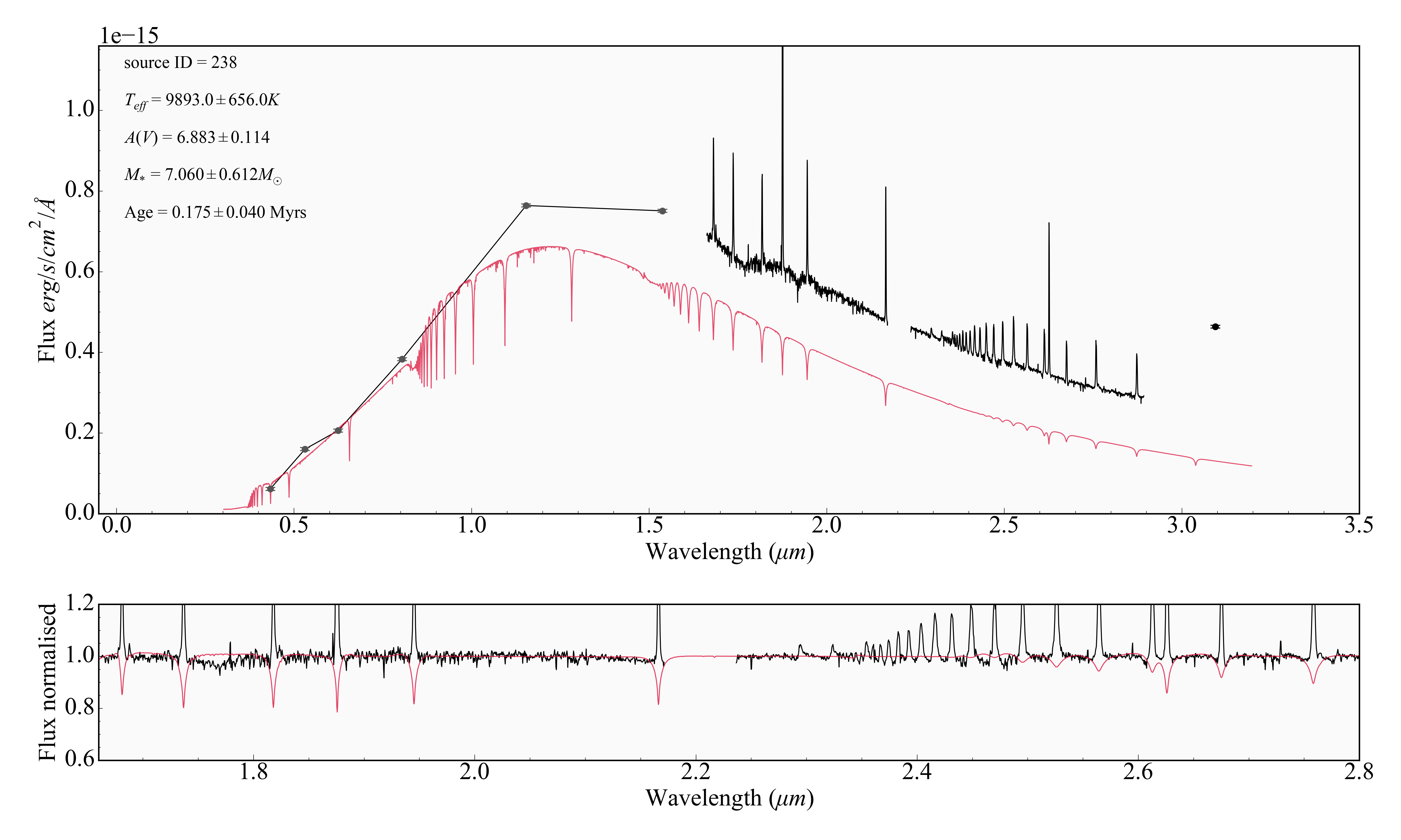
Figure 3: Top panel - SED of source 238 from 0.4-3 $\mu m$. NIRSpec spectrum, with uncertainty represented by error bar (black). HST photometry (grey). Phoenix stellar model (red). Bottom panel - Normalised NIRSpec spectrum (black). Phoenix stellar model (red). Best fitting model shows no metal absorption lines, consistent with the NIRSpec spectrum. All hydrogen absorption lines are filled in by emission. We have removed the bump at $1.71$ $\mu m$ for aesthetic reasons.

5.1 Comparing SED fitting to spectroscopic classification

SED fitting as a method to determine stellar parameters is not as accurate as a full spectroscopic approach. In order to benchmark the accuracy of the parameters returned from the best fitting SEDs, we obtained archival optical spectra for two continuum sources in our sample. These sources are not part of this kinematic analysis, as only a few hydrogen lines are seen in emission. Nonetheless, they have been classified in an identical manner to the five sources being discussed here, and as such should indicate how accurate our SED fitting approach is. Their optical spectra were obtained with MUSE by Kuncarayakti et al. (2016). In their spectra, both $H_{\beta}$ and a portion of the Paschen series are strongly detected in absorption. We fitted their optical spectra to constrain $T_{eff}$ and $A(V)$. Table 2 shows the best fitting $T_{eff}$ and $A(V)$ from the SED fitting and spectroscopic fitting. The best fitting optical spectra for these sources are shown in appendix B.

ID	SED $T_{eff}$(K)	MUSE $T_{eff}$(K)	SED A(V)	MUSE A(V)
152	$6185$	$7200$	3.533	$4.53$
354	$6875$	$7000$	4.842	$5.16$

Table 2: SED fitting compared to spectroscopic fitting

In both cases we underestimated the true $T_{eff}$ of the sources, which have optical spectra consistent with spectral type A. This appears consistent with our indirect arguments given above. Exceedingly high levels of veiling are required to remove metal absorption lines from the NIR spectra of cooler stars. So much so that the entire SED shape would become incompatible with our observations. Invoking a high $T_{eff}$ value naturally explains the lack of metal absorption, and is broadly consistent with the relatively high temperatures that were returned by our SED approach. From all of this, we conclude that sources $238$, $185$ and $823$ are Herbig Ae type stars. It is possible that we have underestimated the temperatures of source $469$ and $251$, which may also be Herbig AeBe type stars. It is unlikely that any of these five sources are cooler than the best fitting SED temperatures.

6 Results - Line kinematics

6.1 Spectral resolution of NIRSpec MSA

The first step in analysing the kinematics of the hydrogen emission lines was to determine the actual spectral resolution of NIRSpec when using the MSA to observe point sources. The often quoted resolving power of $\frac{\lambda}{\Delta\lambda}\sim 2700$ is based on pre-flight calculations, assuming a fully illuminated micro-shutter, with each resolution element being sampled by $2.2$ pixels on the NIRSpec detectors. For point sources however, the resolving power increases by a factor of roughly $\sim 1.5$. To explain this effect, the connection between a micro-shutter and the pixels onto which it projects needs to be understood. The micro-shutters have been designed to project geometrically over two detector pixels, ensuring that for a fully illuminated micro-shutter the line spread function (LSF) is Nyquist sampled (Ferruit et al. 2022). A uniformly illuminated micro-shutter can be imagined as containing an infinite series of point sources. Each of these point sources projects to a slightly different region of the detector. When light is dispersed from each of these point sources, the LSFs of neighbouring points blend together, forming a broader LSF that is composed of many intrinsically narrower LSFs. This blending reduces the fundamental spectral resolution that is achievable with NIRSpec. In the case of a point source, this blending does not occur, as there is only one source of light projecting onto the detector. This means that a higher spectral resolution is achievable when observing point sources compared to extended sources. This has the side effect that, for point sources, the LSF is not Nyquist sampled at any wavelength.
Given that all of our sources are point sources, the actual spectral resolution achieved for our observations needed to be determined if we wished to analyse the kinematics of the emission lines. We have used the JWST-MSAfit software from de Graaff et al. (2024) to do this. This software provides forward modelling and fitting of simulated MSA data. It allows the user to first select a grating and filter combination, and then define a source (extended or point-like) and place it in a specified micro-shutter at a specified position within that micro-shutter. A spectrum with uniformly spaced emission lines is generated from this. The $FWHM$ of the emission lines are measured in order to determine what the resulting resolving power is at each wavelength. The estimated uncertainty of this approach is expected to be between $10-20\%$ (de Graaff et al. 2024). Using this tool we have determined that the actual resolving power for our sources is $\frac{\lambda}{\Delta\lambda}\sim 4300$, at $\lambda=1.875\mu m$. This corresponds to a FWHM of $\sim 70\pm 14kms^{-1}$, assuming an uncertainty of 20 %.

6.2 FWHM of hydrogen emission lines

Emission lines are broadened through numerous processes, including natural broadening, thermal broadening, rotational (Doppler) broadening and pressure broadening (eg. Stark broadening). In general, these processes contribute $\leq 100kms^{-1}$ of broadening (although in some cases it can be significantly more as we discuss in section 7.5). In the circumstellar environment, gas moving at high velocities due to infall and outflow processes can introduce significant line broadening, of order hundreds of $kms^{-1}$. As such, the FWHM of emission lines from PMS stars is typically interpreted as reflecting the velocity of the gas that produced the emission line. Narrow lines then originate from slow moving gas, e.g., molecular outflows of $H_{2}$ and $CO$ with $FWHM\leq 10km/s^{-1}$, while broad lines originate from high velocity gas e.g. H I, $FWHM\geq 100kms^{-1}$. Figure 4 shows the FWHM of the Paschen, Brackett and Pfund emission lines from source $238$. We have also plotted the resolution of NIRSpec obtained in section 6.1. Although we focus on source 238 for the remainder of this analysis and discussion, the same general kinematic behaviour is seen for all five sources. The FWHM diagrams of the other sources can be seen in the Appendix A.

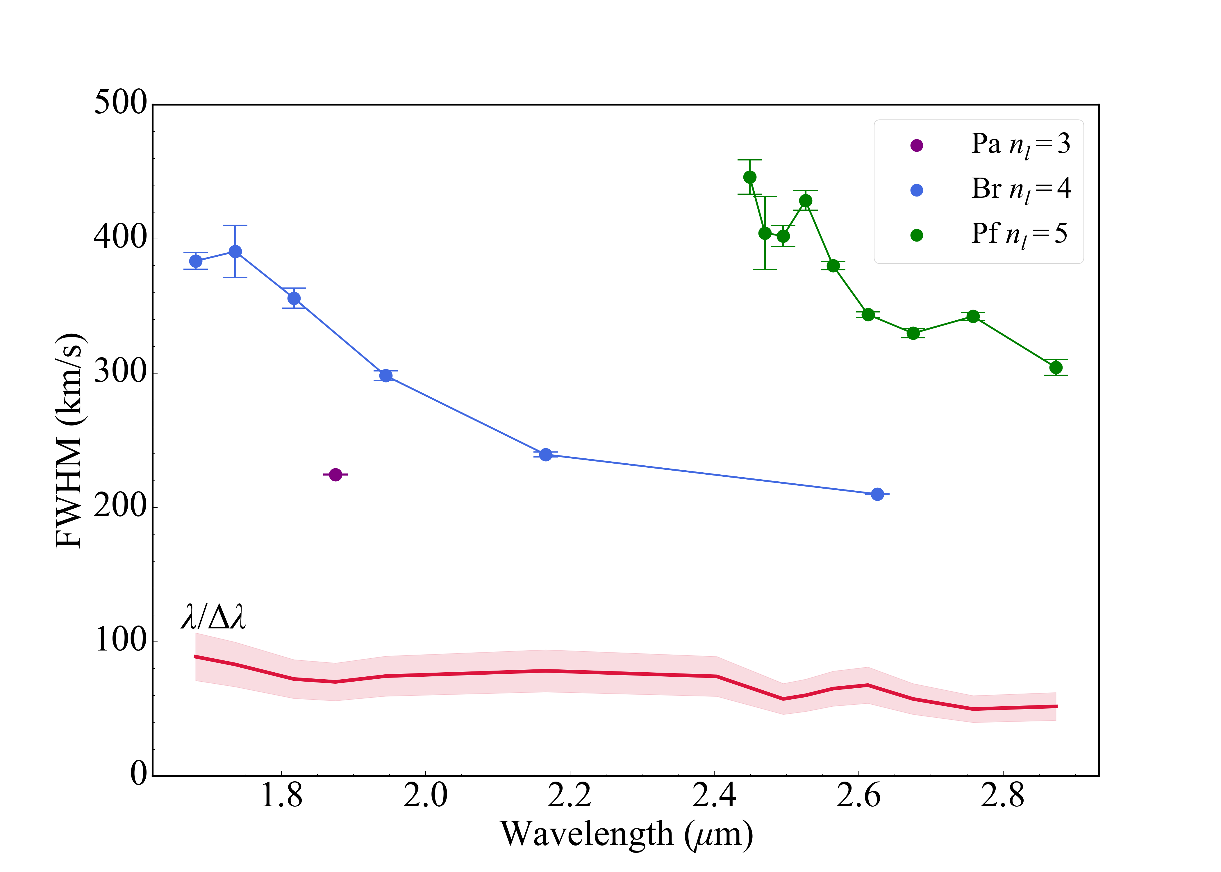
Figure 4: The FWHM of each hydrogen emission line of source $238$. Paschen series (purple). Brackett series (blue). Pfund series (green). Expected instrumental resolution (red). Systematic uncertainty of spectral resolution (pale red).

A striking relationship is immediately apparent. The FWHM for a given series tends to decrease with increasing wavelength. This is evidently not purely a wavelength effect, as lines from different series with similar wavelengths have drastically different FWHMs. Rather, the trend appears to follow the upper energy level $n_{up}$ of the transition, with higher order transitions (electrons falling from high $n_{up}$) tending to have larger FWHMs. This result suggests that the high excitation lines come from the fastest moving gas, while lower excitation lines come from gas with somewhat lower velocities. The Pfund series displays some significant scatter, as the highest order lines are bunched close together in wavelength and are much weaker than the Brackett or Paschen series. This makes the measurement of these lines challenging in terms of identifying the true level of the continuum, and therefore obtaining reliable fits to the weakest lines. The kinematic trend is dramatic enough that it is still clearly present despite these challenges.

6.3 Line profile optical depths

An additional way to investigate the kinematics of the hydrogen emission lines is to take the ratio of two spectrally resolved line profiles, in order to probe the optical depth of the lines at various velocities. This analysis is akin to that performed by Bunn et al. (1995) and Lumsden et al. (2012). We have used two pairs of lines in this analysis, $\frac{Br_{11}}{Br_{6}}$ and $\frac{Pf_{17}}{Pf_{11}}$. These lines were chosen so that the optical depth of the Brackett and Pfund series could be compared to each other, as well as to compare lines with significantly different $n_{up}$/excitation energies. If the lines are optically thin, the line profile ratio should be consistent with Case B recombination (Baker & Menzel 1938). We have used the line ratios computed under Case B recombination from Storey & Hummer (1995) for the Brackett and Pfund lines. If the emission is completely optically thick, then the ratio simply becomes a function of wavelength and emitting area,

$$\centering\frac{I_{1}}{I_{2}}=(\frac{\lambda_{2}}{\lambda_{1}})^{4}(\frac{S_{1}}{S_{2}})\@add@centering$$ (1)

where $I$ is the intensity of the emission line, $\lambda$ is the wavelength of the line, and $S$ is the emitting surface area.
One would expect that the emitting area $S$ should be smaller for the high excitation lines. The degree of excitation in the gas increases closer to the central star. A relatively small portion of gas in the accretion flow or wind is excited enough to produce high excitation lines. A larger, more extended portion of this gas farther away from the central star is only excited enough to produce lower order lines. For simplicity however, we will assume that $S_{1}=S_{2}$, which provides us with a lower limit to the optically thick ratio for each pair of lines. Line ratios that lie between the completely optically thick and optically thin regimes correspond to only one of the two lines being optically thick.
Figure 5 shows the optical depth diagrams for $\frac{Br_{11}}{Br_{6}}$ and $\frac{Pf_{17}}{Pf_{11}}$. Due to the limited number of pixels sampling each line, we interpolated the line profiles so that they could be accurately centred and aligned. As a result, it is important not to overinterpret these diagrams. Small scale variations in the line profile ratio could be artificial, and likely do not reflect real physical changes in the line optical depth over small velocity scales. Only the overall shape of the line profile ratio should be considered, and where it is clearly optically thin, and clearly optically thick.

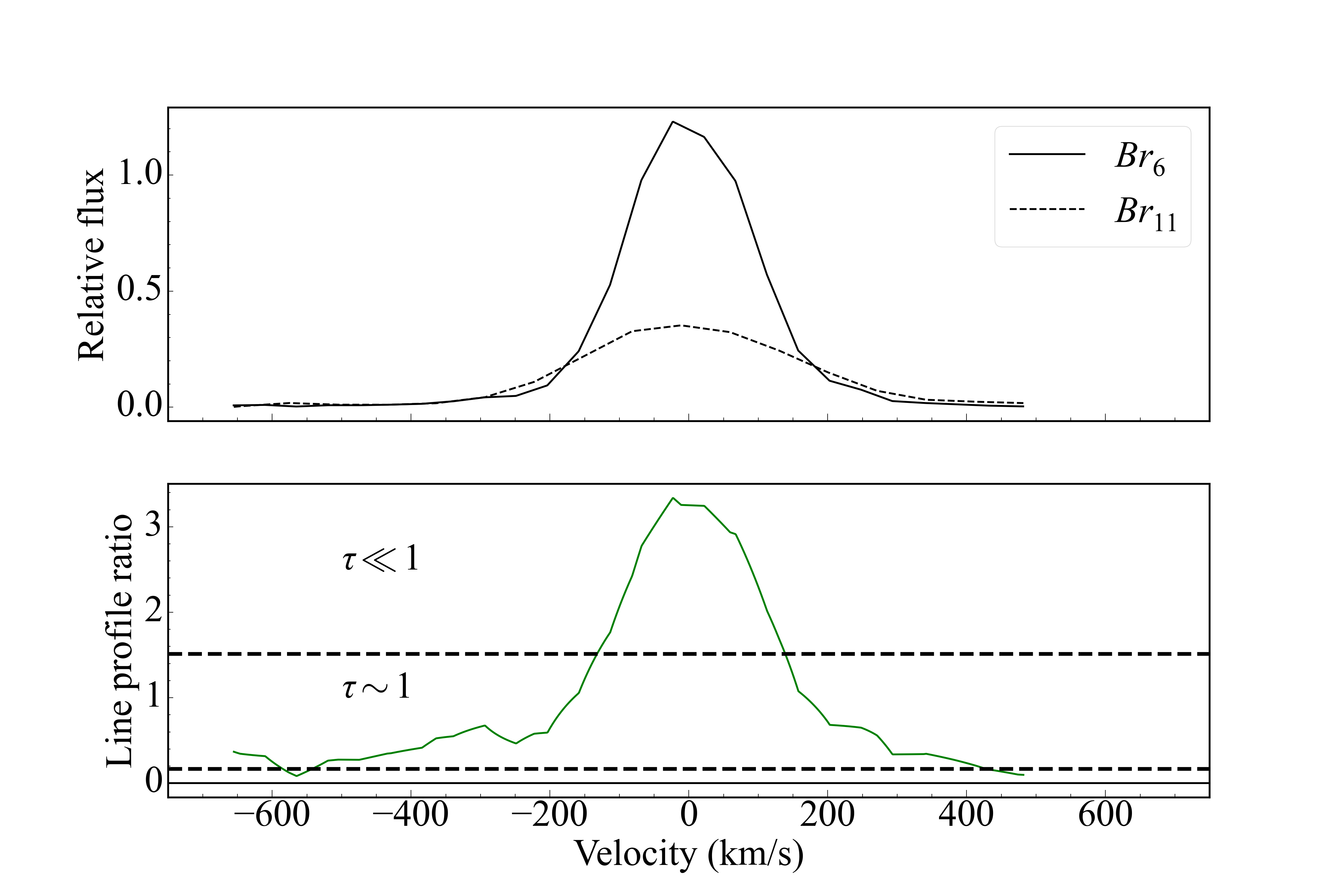
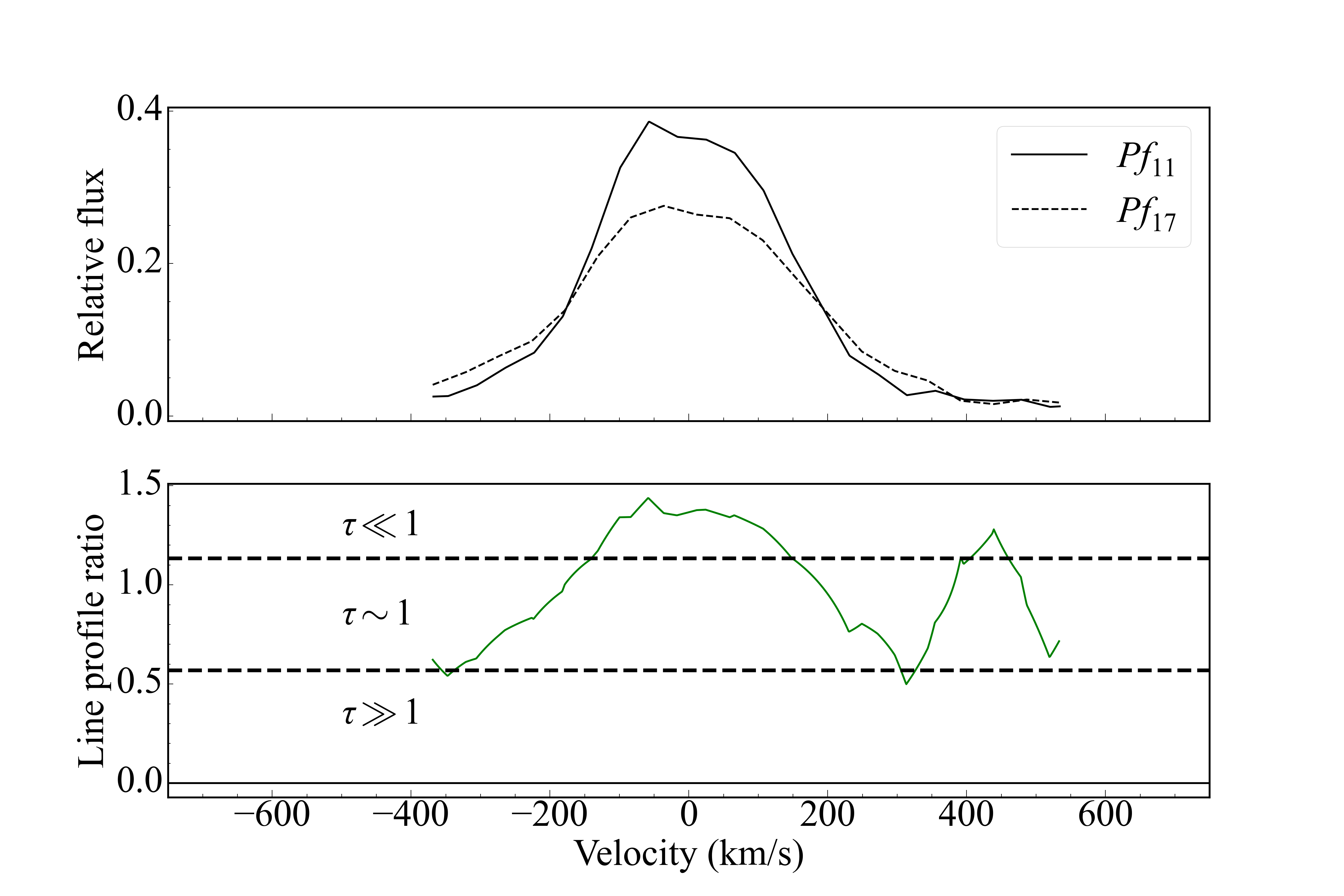
Figure 5: Optical depth diagrams for spectrally resolved emission lines. Top: The line profiles $Br_{11}$ and $Br_{6}$ are shown as the solid and dashed black lines, respectively. The line profiles are plotted on a velocity scale, with each line centred at its rest wavelength. Underneath, the green solid line shows the line profile ratio $\frac{Br_{11}}{Br_{6}}$. The horizontal dashed black lines demarcate optically thin and optically thick areas. Bottom: Same as above but for $Pf_{17}$ and $Pf_{11}$.

From these optical depth diagrams, we can see that for both the Brackett and Pfund lines, the lowest velocity components of the lines are consistent with optically thin emission. The wings of the lines however quickly become optically thick, with the highest velocity components of each line showing the most optically thick ratio. Interestingly the Pfund lines show a much larger fraction of the line profile ratio in the optically thick regime compared to the Brackett lines. We also note here that the line profile ratios include some continuum regions. The ratio is not physically meaningful at these velocities, because we are no longer sampling the line profile. For the Brackett line, this refers to velocities beyond $\pm 200km/s$ and for the Pfund series $\pm 350km/s$.

7 Discussion - the origin of circumstellar hydrogen emission lines

7.1 Magneto-centrifugal winds?

The two most common origins suggested for hydrogen emission lines from young stars is either the accretion flow, and/or an accelerating magneto-centrifugal disk wind (Muzerolle et al. 1998a; Kurosawa et al. 2006; Lima et al. 2010), also referred to as a magneto hydrodynamical (MHD) wind. If a magneto-centrifugal wind were the dominant line emission mechanism, the high excitation lines should come preferentially from close to the launching point near the disk/stellar surface, where the gas is hottest and most strongly irradiated by the central star. The gas at this point should then have a low velocity, as it has not yet experienced much acceleration. Likewise, one would expect the lower excitation lines to come preferentially from the gas at greater distances from the star, as the irradiation/temperature is still sufficient to produce low excitation lines, and the effective emitting area is significantly larger than at the star/disk surface. This gas would then have a high velocity as it has experienced more acceleration. In this picture, the high excitation lines should display narrow profiles, and the low excitation lines should display broad profiles, owing to the velocity of the gas that predominantly produces them.

This general trend has been observed towards very young Class I protostars, known to exhibit powerful jets and outflows (Nisini et al. 2004), with the lower excitation $Br_{7}$ line appearing significantly broader than the higher excitation lines $Br_{12}$ and $Br_{13}$. We have obtained archival JWST NIRSpec IFU data of source $TMC1A$, a class I protostar, with a spatially resolved outflow (see Harsono et al. (2023) for a full discussion of this source). These observations used the same grating and filter combination as our own. Given that the source is spatially resolved, we expect that the resolving power of these observations are intermediate between our own and that of a uniformly illuminated aperture. We have performed the same kinematic analysis on these data, extracting the flux from the datacube using a $3\times 3$ pixel aperture. We have made use of only the Paschen and Brackett lines. The Pfund lines in this case are either too weak, or located in the strong $H_{2}0$ absorption feature at $3.08\mu m$, and therefore could not be used. Figure 6 shows the resulting FWHMs for each line.

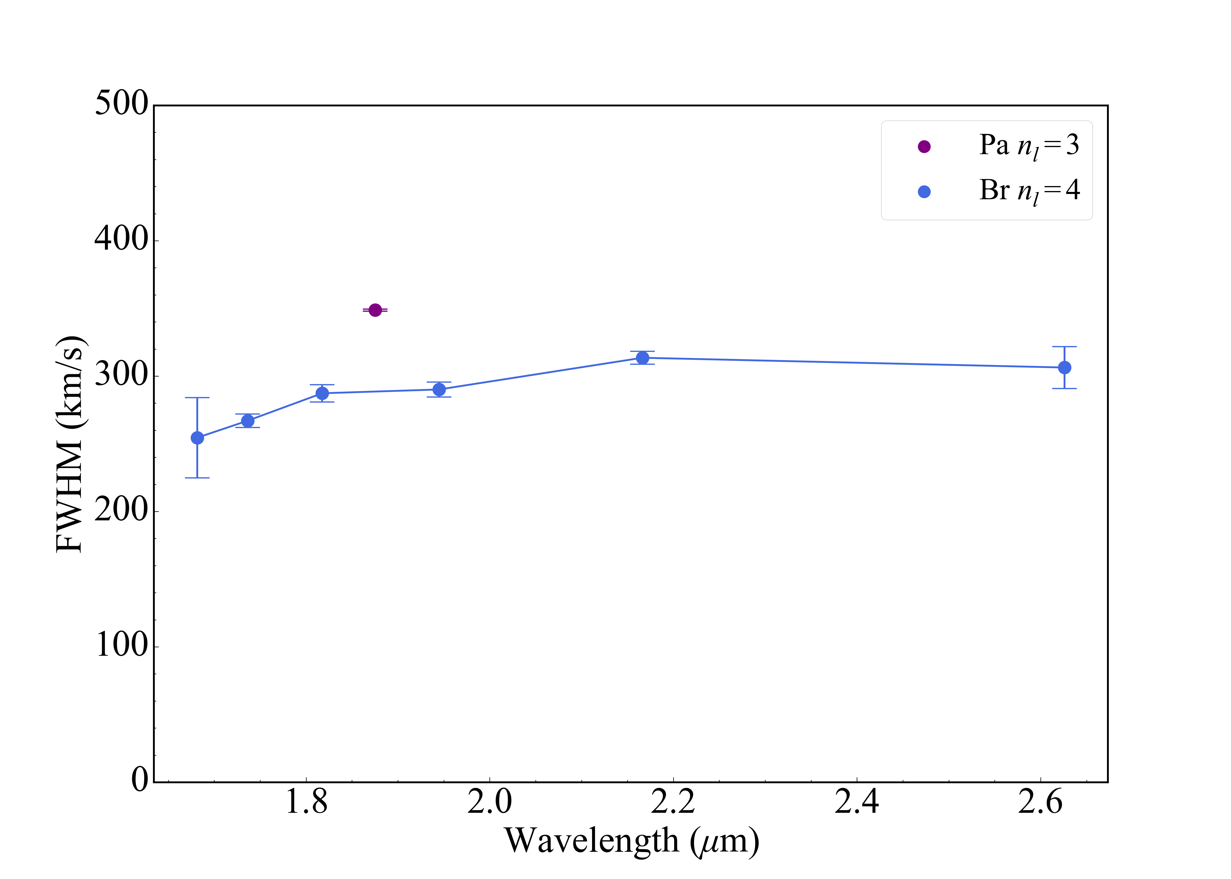
Figure 6: The FWHM of each hydrogen emission line of source $TMC1A$. Paschen series (purple). Brackett series (blue).

The trend seen here is clear. The highest excitation line $Br_{11}$ has the smallest FWHM, $\sim 250kms^{-1}$, while the lowest excitation line $Pa_{\alpha}$ has the highest FWHM, $\sim 350kms^{-1}$.
In an accelerating wind, the highest velocity gas far away from the star should have low optical depth, as the density has fallen off by several orders of magnitude compared to the star/disk surface (Lima et al. 2010). Conversely, the gas at the launching point of the wind, with much higher density, should have higher optical depth. The resulting line profile ratios would then show higher optical depth in the line core, becoming optically thinner towards the wings.
In figure 7, we show the line profile ratio for TMC1A. In this case we have used $Br_{10}$, as $Br_{11}$ is too weak to be measured reliably. The optical depth diagram of TMC1A is essentially inverted compared to source $238$. The line core is the closest to optically thick, while the wings are firmly in the optically thin regime. We note that we have not attempted to correct the spectrum of TCM1A for extinction. Doing so would cause the flux of $Br_{10}$ to increase by a greater amount than $Br_{6}$, pushing the core of the line profile ratio further into the optically thick regime.
The kinematic trends seen here suggest that the hydrogen emission lines in TMC1A come predominantly from an accelerating wind, which is supported by the spatially resolved outflow seen towards this source, as well as the presence of other wind and outflow tracers such as $H_{2}$ and $Fe[II]$ emission. This conclusion was also reached by the authors (Harsono et al. 2023).

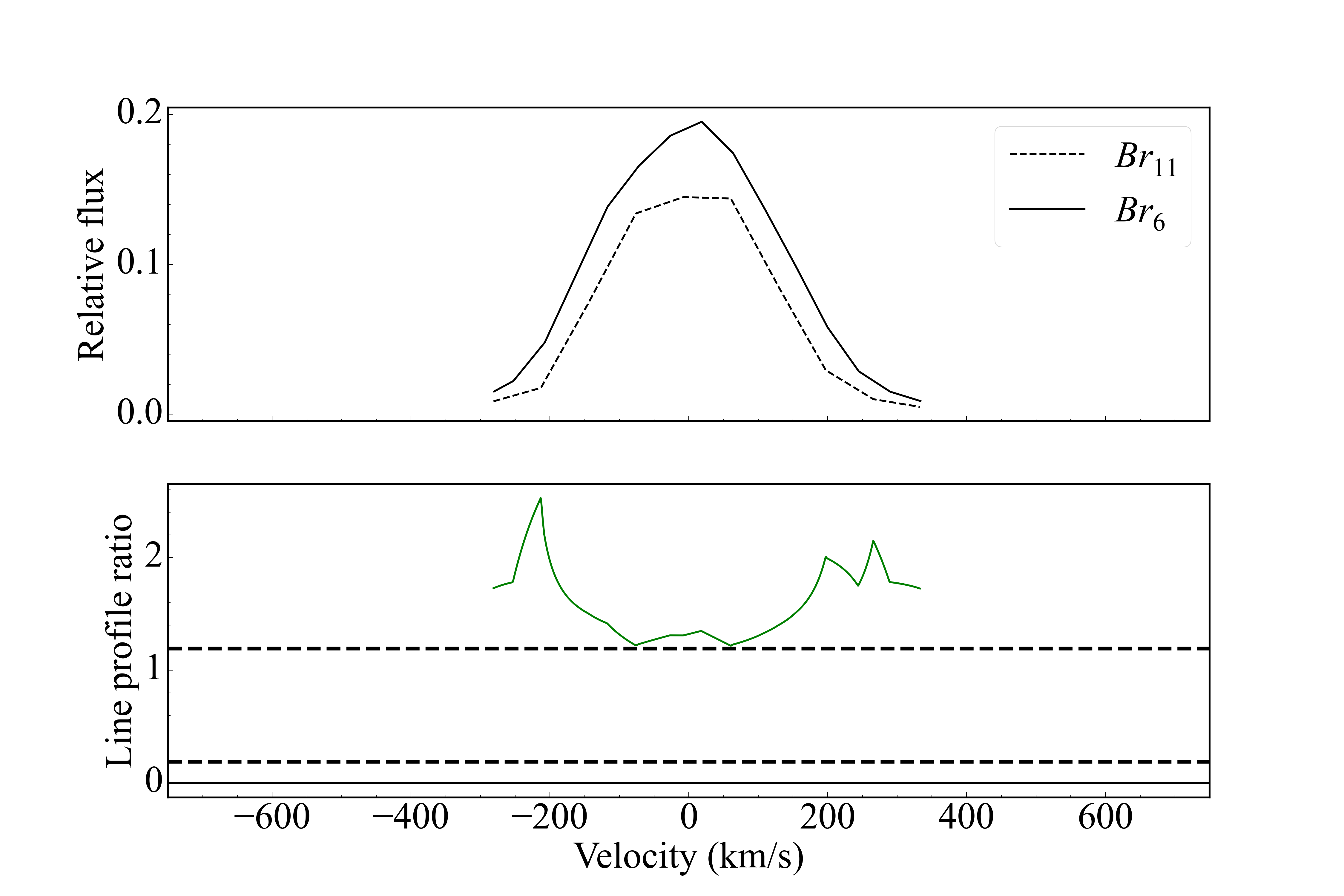
Figure 7: The line profiles $Br_{10}$ and $Br_{6}$ are shown as the solid and dashed black lines respectively. The green solid line shows the line profile ratio $\frac{Br_{10}}{Br_{6}}$.

7.2 Magnetospheric accretion?

The trends seen for TMC1A in terms of kinematics and optical depth are in total contrast to what we observed towards our sources in NGC 3603. Thus, we now consider the accretion scenario as the dominant line emission mechanism for the sources in NGC 3603. In this scenario, the high excitation lines should come preferentially from gas in the accretion flow close to the stellar surface. Here the conditions are preferable for high excitation line emission, as the gas is strongly irradiated by the star and the temperature is significantly higher than at the disk surface (Lima et al. 2010). This gas would move with high velocity, as it has been in near free-fall from the disk surface, and hence has experienced significant acceleration. The low excitation lines should come preferentially from gas at the base of the accretion flow on the disk surface. Here the temperature and irradiation are still sufficient to produce low excitation emission lines, and due to the funnel like geometry of the accretion flow the effective emitting area is larger at the base of the flow compared to just before it hits the stellar surface (e.g. Muzerolle et al. 1998a). This gas would move with a lower velocity as it has yet to experience much acceleration. In this picture, the high excitation lines should display broad profiles, as they come from the highest velocity gas, while the low excitation lines should display narrow profiles, as they come from the lower velocity gas. This is consistent with the emission line profiles that we have measured across three spectral series, for over $15$ hydrogen emission lines for source 238, as well as for the other four sources in this sample.
The fastest moving gas in an accretion flow should also be the most optically thick, as the density of the gas in the accretion flow increases as it approaches the central star. Again, this is consistent with the line profile ratios measured for source $238$ and the others. Based on the combination of line kinematics and optical depth diagrams, we favour magnetospheric accretion as the dominant source of line emission over an accelerating stellar/disk wind for our sources. This claim is bolstered by the fact that none of the typical outflow/jet tracers are present in our spectra such as $H_{2}$, which may suggest a lack of any substantial outflow.

7.3 The magnetospheric accretion paradigm in Herbig AeBe stars

The observed Paschen, Brackett, and Pfund lines originating from the magnetospheric accretion flow is a somewhat unexpected result. It is surprising that disk wind signatures are not detected in either the kinematic analysis or from the presence of outflow signatures/species. Tambovtseva et al. (2016) performed Non-LTE modelling to investigate whether accretion or winds were the dominant emission mechanism for $Br_{7}$ from Herbig AeBe stars, concluding that disk winds do indeed dominate. This was supported by a subsequent spectro-interferometric observational study of MWC 120 by Kreplin et al. (2018), who concluded again that $Br_{7}$ is formed predominantly in an extended wind around the star, not the compact magnetosphere. Kraus et al. (2008) employed spectro-interferometry to try and spatially resolve the emission region of $Br_{7}$. They found that of the five sources observed, only one, source HD98922, displayed compact $Br_{7}$ emission, consistent with an origin from a magnetospheric accretion flow.

The origin of hydrogen emission lines from Herbig AeBe stars is not definitively known, and likely depends on multiple parameters including the age, mass, and accretion rate of the central source. We are not aware of any other studies in the literature that have investigated the kinematic properties of hydrogen emission lines systematically as we have presented here, and suggest that this approach could be helpful in distinguishing between different emission line mechanisms. In the next section we explore other mechanisms not yet discussed that could also explain the kinematic measurements that have been made.

7.4 Alternative line emission mechanisms

We have focused on accretion and magneto-centrifugal star/disk winds to try and explain the hydrogen emission lines observed towards our Herbig AeBe stars. There are, however, alternative mechanisms that could potentially explain the kinematic and optical depth results that have been presented so far. They include:

1. Line driven stellar winds.

2. Hot gaseous inner disk.

3. Internal/external photoevaporative winds.

4. Boundary layer accretion

7.4.1 Line-driven stellar wind

Line driven stellar winds are common around massive stars, whose stellar luminosity exceeds the Eddington limit (Abbott 1982). Here stellar photons impart enough momentum to gas on the stellar surface to overcome the gravitational potential of the star, driving a decelerating wind. A decelerating wind could qualitatively match the kinematic results presented. However, although our stars are more massive and hotter than CTTS, their luminosities are still well below the Eddington limit, and hence line driven winds are not expected around our sources.

7.4.2 Hot inner gaseous disk.

The hot inner gaseous disk may contribute towards the observed hydrogen emission lines. In their seminal work Muzerolle et al. (2004) showed that the inner disk is expected to become an important contributor of emission for mass accretion rates of $\geq 10^{-7}M_{\odot}$yr^-1, and all Herbig AeBe stars considered here have accretion rates above this level. The inner disk as the dominant source of emission is also supported by the presence of $CO$ bandhead emission detected towards three of the five sources (see figure 1), which likely arises from the warm inner disk (e.g. Ilee et al. 2013). The detection of $CO$ bandhead emission suggests that there is still ample gas in the inner disk around the star. If the hydrogen lines were formed in the inner disk, rotational broadening would likely be the dominant line broadening mechanism, since it is the only mechanism capable of producing the FWHMs that we have measured. However, rotational broadening produces a characteristic double-peaked profile in emission lines and even with the moderate spectral resolution of NIRSpec double-peaked profiles should be detected, even at low inclinations.
We created a simple toy model of $Br_{7}$ emission from the inner disk to demonstrate this. Taking the stellar parameters for source 238 from section 5, we modelled a disk in Keplerian rotation around a star with $M_{*}=7M_{\odot}$ and $R_{*}=12R_{\odot}$. The disk inner radius $R_{inner}$ was set to $2R_{*}$, and the outer radius $R_{outer}$ was set to $1AU$, equivalent to $18R_{*}$, with 100 steps between the two. The Keplerian velocity field was used to calculate the Doppler shift experienced by the line for each step in radius. We modelled the $Br_{7}$ emission line as an unresolved Gaussian (FWHM = 50 km s^-1). A Doppler shift was applied to the Gaussian for each step in radius and theresulting Gaussians were summed together, producing the final emission line profile, normalised to its peak intensity. The resulting line profile was double peaked. We then downgraded the double peaked profile to the spectral resolution of NIRSpec at the wavelength of $Br_{7}$ and also injected Gaussian noise into the line, at the level of $2\%$ (this is the noise level measured in the actual spectrum of source 238). The noisier, lower resolution line profile still exhibits clear double peaked emission line profiles down to inclinations of $20\deg$. Below this inclination, the double peaked profile disappears and the resulting FWHM reduces to $\sim 100$ km s^-1. In figure 8, the profiles of $Br_{7}$ are shown at inclination angles of $10^{\circ}$, $30^{\circ}$, and $70^{\circ}$, respectively.

Figure 8: The line profile of $Br_{7}$ if it were to originate in a keplerian rotating inner disk. Inclination angles are $10^{\circ}$, $30^{\circ}$, and $70^{\circ}$.

A similar result was also found by Wilson et al. (2022), who computed rotationally broadened emission line profiles for $Br_{7}$ for different rates of rotation and inclinations. They showed that for rotational velocities of $\sim 130$ km s^-1, which is typical for Herbig AeBe stars (Böhm & Catala 1995), the peak-to-peak separation of double-peaked $Br_{7}$ is $\sim 100$ km s^-1 for a viewing inclination of $20^{\circ}$, which would be resolved at NIRSpec’s resolution. Therefore, based on the lack of double peaked emission lines in our spectra, we can confidently rule out emission from the inner disk as the dominant line emission mechanism.

7.4.3 Internal photoevaporative wind.

X-ray and far-ultraviolet (FUV) radiation from the central star can drive thermal, decelerating winds from the disk surface (Owen et al. 2012). These winds can produce hydrogen emission lines that could in principle display the same kinematic trends that we have measured. Ercolano & Owen (2010) computed theoretical line luminosities for many hydrogen recombination lines forming in a photoevaporative wind. For $Br_{7}$, the line luminosity $\frac{L(Br_{7})}{L_{\odot}}$ ranges from $3.05\times 10^{-9}$ erg s^-1 to $1.26\times 10^{-7}$ erg s^-1, for X-ray luminosities $L_{X}$ of $10^{29.3}$ erg s^-1 to $10^{30.3}$ erg s^-1, respectively. These calculations were carried out for CTTS. X-ray luminosities are generally higher for Herbig AeBe stars compared to CTTS, with $L_{X}$ up to $\sim 10^{32}$ erg s^-1 (Zinnecker & Preibisch 1994; Hamaguchi et al. 2005). This would likely lead to larger internal photoevaporative $Br_{7}$ line luminosities. However, these values are still $4-6$ orders of magnitude lower than the line luminosities measured for $Br_{7}$ in our sample. As such, we do not expect that internal photoevaporative winds could dominate the hydrogen line emission for our sources.

7.4.4 External photoevaporative wind.

Since our sources are located in a massive star forming region, external photoevaporation could contribute towards the hydrogen line emission. The massive stars of spectral type O and B at the centre of NGC 3603 irradiate our sources, which can result in a thermally driven cocoon of gas and dust escaping the protoplanetary disk, with an ionisation front around the source resulting from extreme-ultraviolet photons. This cocoon morphology is seen commonly around the PMS stars in Orion known as proplyds (e.g. Ricci et al. 2008). At a distance of $7.2$ kpc, it is not possible to spatially resolve these sources with current facilities, and so it is not obvious whether they possess this cocoon morphology or ionisation front. However, in the case of Orion, where the detection of these features is unambiguous, the hydrogen emission lines from the ionisation front resemble the nebular emission lines, with narrow line profiles (FWHM $\leq 50$ km s^-1). Furthermore, our nebular subtraction has removed any contribution from the ionisation front thanks to the He I scaling method, as the He I emission line strength would have a contribution from both the extended nebular gas as well as the ionisation front. By removing the He I emission, we have removed the contribution of both the nebular emission and any possible ionisation front emission. Based on the broad lines that we measure from our sources, and the subtraction method that we have developed and employed, an externally driven photoevaporative wind cannot be the dominant emission line mechanism in this case.

7.4.5 Boundary-layer accretion.

An alternative accretion mechanism that has been invoked for Herbig AeBe stars is boundary layer accretion. In this scenario, the magnetic field from the star is either entirely absent or is too weak to truncate the protoplanetary disk. The inner disk connects to the stellar surface via the so-called boundary layer. Disk material must reduce its Keplerian velocity to match the stellar rotational velocity. This reduction in velocity, and hence kinetic energy, is converted into radiation producing the observed accretion luminosity (Mendigutía 2020; Wichittanakom et al. 2020). Given that material must decelerate in order to be accreted, with the highest excitation gas then moving at the slowest velocity, the observed kinematic trends cannot be explained with a boundary layer accretion scenario.

7.5 Stark broadening

Up to now, we have assumed that the dominant line broadening mechanism is Doppler broadening, due to the high velocity bulk motion of the gas. This is often invoked to explain the line widths for CTTS and Herbig AeBe stars, as the velocities from infalling and outflowing material match the line widths well (e.g. Muzerolle et al. 2004). In some cases, line widths have been measured that are too broad to be consistent with Doppler broadening. Muzerolle et al. (1998a) suggest that Stark broadening could explain the high velocity wings observed towards $H_{\alpha}$, extending out as far as $\pm 500$ km s^-1. None of the lines in our sample exhibit such broad wings, with the broadest lines having wings out to $\pm 300$ km s^-1. Since these line widths can be easily explained with Doppler broadening, we do not necessarily need to invoke another broadening mechanism, but we felt that a short discussion was warranted because as previous studies have suggested that Stark broadening could be important for Brackett lines (Bunn et al. 1995; Lumsden et al. 2012). For instance, Wilson et al. (2022) computed Stark broadened emission line profiles for $H_{\alpha}$, $Pa_{5}$, $Pa_{6}$ and $Br_{7}$ and found that, while the effect was significant for $H_{\alpha}$, the NIR lines were negligibly affected. Muzerolle et al. (1998a) reached a similar result, finding that Stark broadening can impact $H_{\alpha}$ significantly for high densities $n_{H}\geq 10^{12}cm^{-3}$ and temperatures $T\sim 10000$K, but the effect drops off quickly, with $H_{\beta}$ experiencing $50\%$ less broadening compared to $H_{\alpha}$. Based on these results, as well as the lack of extremely high velocity line wings in our observations, we do not expect that Stark broadening contributes significantly to our line widths.

8 Conclusions

We have presented JWST NIRSpec spectra of five intermediate mass sources located in the massive star forming region NGC 3603, three of which are Herbig Ae stars. Their spectra exhibit many recombination lines, mostly from H I, and lack any detectable absorption lines from their underlying photospheres. Three of the five sources exhibit CO bandhead emission. We have performed a kinematic analysis on the multiple series of hydrogen emission lines to try and constrain where the line emission originates. Based on the FWHM and optical depth of the spectrally resolved emission lines, we favour an origin in the magnetospheric accretion flow, rather than in a magneto-centrifugal wind. This result provides new observational support to the existence of a magnetically driven accretion mechanism around Herbig Ae stars, which can dominate the line emission from these sources. With a small sample size of five, it is unwise to draw generalised conclusions from these sources alone. As more of these higher mass sources are observed with NIRSpec in the coming years, it will be possible to test the magnetospheric paradigm kinematically with a more statistically robust sample.

Appendix A FWHM diagrams

Figure 9: FWHM of each hydrogen emission line. (Top left) source 185. (Bottom left) source 251. (Top right) source 469. (Bottom right) source 823.

Appendix B MUSE Spectra best fits

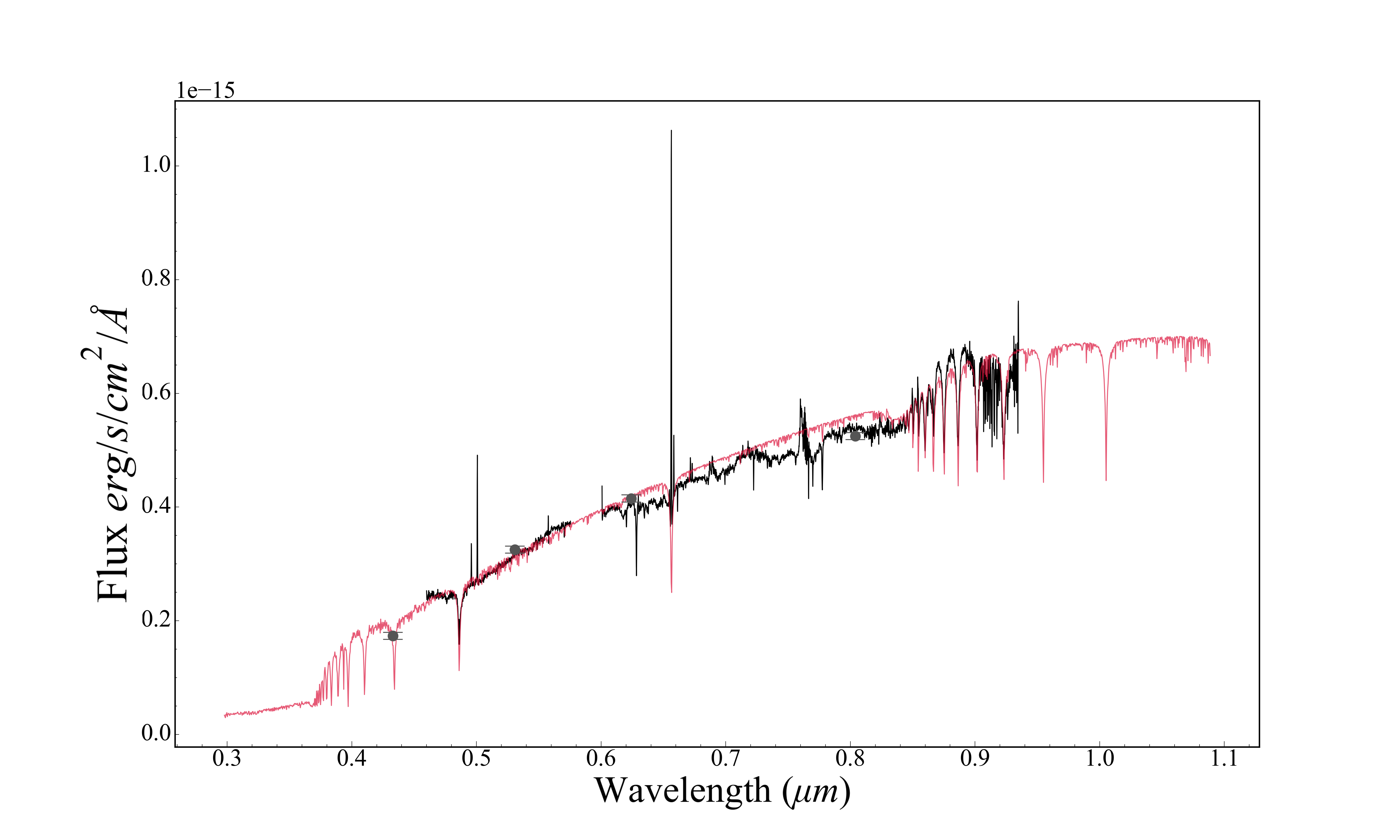
(a) Best fitting optical model spectrum for source $152$ based on it’s MUSE spectrum. (Black) MUSE source spectrum. (Red) best fitting model spectrum. (Grey) HST photometry.

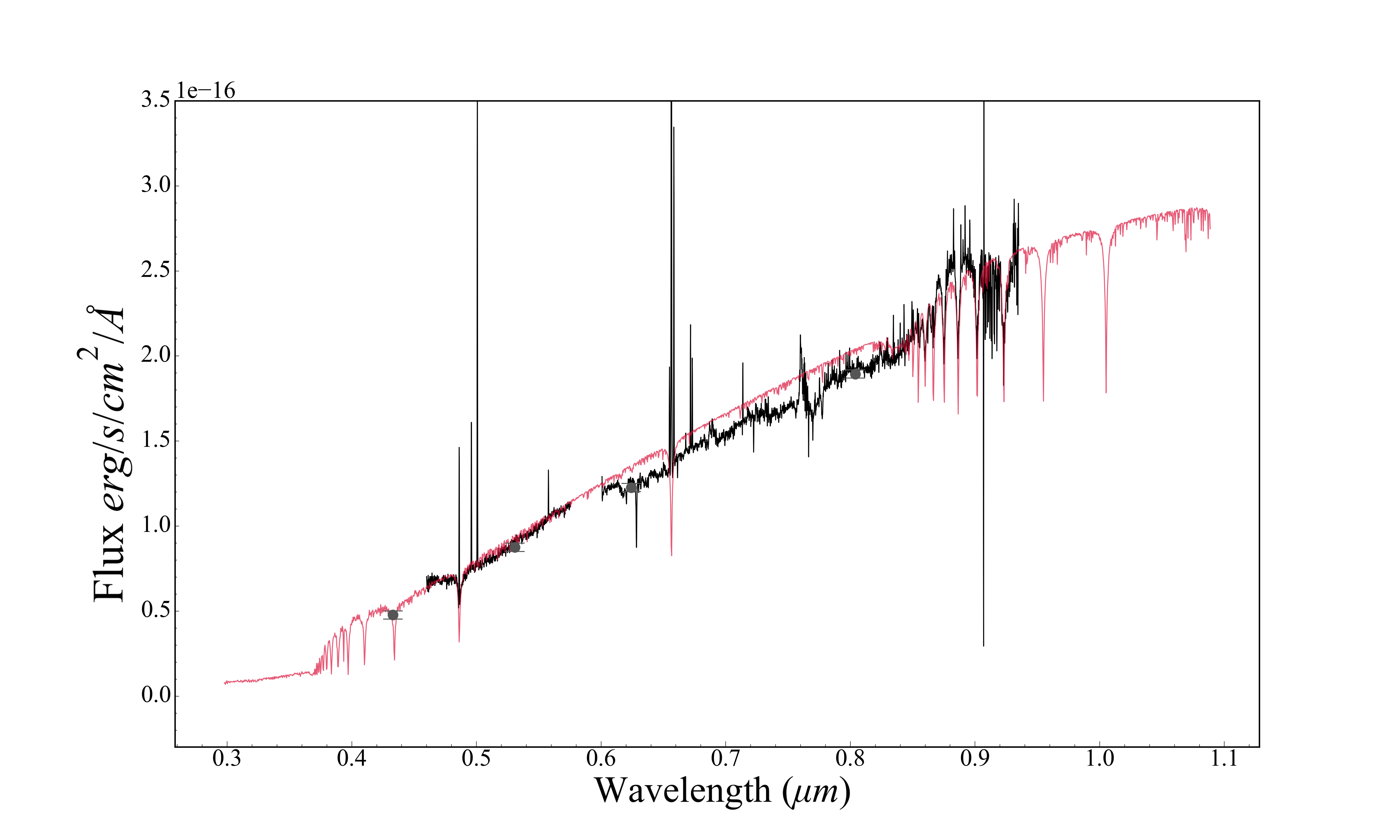
(b) As before for source $354$.

References

- Abbott (1982) Abbott, D. C. 1982, Astrophysical Journal, Part 1, vol. 259, Aug. 1, 1982, p. 282-301., 259, 282
- Alcalá et al. (2017) Alcalá, J., Manara, C., Natta, A., et al. 2017, Astronomy & Astrophysics, 600, A20
- Alcalá et al. (2014) Alcalá, J., Natta, A., Manara, C., et al. 2014, Astronomy & Astrophysics, 561, A2
- Alves de Oliveira et al. (2018) Alves de Oliveira, C., Luetzgendorf, N., Ferruit, P., & Rawle, T. 2018
- Baker & Menzel (1938) Baker, J. G. & Menzel, D. H. 1938, Astrophysical Journal, vol. 88, p. 52, 88, 52
- Bell et al. (2013) Bell, C. P., Naylor, T., Mayne, N., Jeffries, R., & Littlefair, S. 2013, Monthly Notices of the Royal Astronomical Society, 434, 806
- Blandford & Payne (1982) Blandford, R. D. & Payne, D. 1982, Monthly Notices of the Royal Astronomical Society, 199, 883
- Böhm & Catala (1995) Böhm, T. & Catala, C. 1995, Astronomy and Astrophysics, v. 301, p. 155, 301, 155
- Bouvier et al. (2007) Bouvier, J., Alencar, S., Boutelier, T., et al. 2007, Astronomy & Astrophysics, 463, 1017
- Bunn et al. (1995) Bunn, J., Hoare, M., & Drew, J. 1995, Monthly Notices of the Royal Astronomical Society, 272, 346
- Cauley & Johns-Krull (2015) Cauley, P. W. & Johns-Krull, C. M. 2015, The Astrophysical Journal, 810, 5
- de Graaff et al. (2024) de Graaff, A., Rix, H.-W., Carniani, S., et al. 2024, Astronomy & Astrophysics, 684, A87
- Drew et al. (2019) Drew, J., Monguió, M., & Wright, N. 2019, Monthly Notices of the Royal Astronomical Society, 486, 1034
- Ercolano & Owen (2010) Ercolano, B. & Owen, J. E. 2010, Monthly Notices of the Royal Astronomical Society, 406, 1553
- Ferruit et al. (2022) Ferruit, P., Jakobsen, P., Giardino, G., et al. 2022, Astronomy & Astrophysics, 661, A81
- Frank et al. (2014) Frank, A., Ray, T., Cabrit, S., et al. 2014, Protostars and planets VI, 451
- Gullbring et al. (1998) Gullbring, E., Hartmann, L., Briceno, C., & Calvet, N. 1998, The Astrophysical Journal, 492, 323
- Hamaguchi et al. (2005) Hamaguchi, K., Yamauchi, S., & Koyama, K. 2005, The Astrophysical Journal, 618, 360
- Harsono et al. (2023) Harsono, D., Bjerkeli, P., Ramsey, J., et al. 2023, The Astrophysical Journal Letters, 951, L32
- Hartmann et al. (2016) Hartmann, L., Herczeg, G., & Calvet, N. 2016, Annual Review of Astronomy and Astrophysics, 54, 135
- Herczeg & Hillenbrand (2008) Herczeg, G. J. & Hillenbrand, L. A. 2008, The Astrophysical Journal, 681, 594
- Horne (1986) Horne, K. 1986, PASP, 98, 609
- Ilee et al. (2013) Ilee, J., Wheelwright, H., Oudmaijer, R., et al. 2013, Monthly Notices of the Royal Astronomical Society, 429, 2960
- Johns-Krull (2007) Johns-Krull, C. M. 2007, The Astrophysical Journal, 664, 975
- Kageyama & Sato (1997) Kageyama, A. & Sato, T. 1997, Physical review E, 55, 4617
- Koenigl (1991) Koenigl, A. 1991, Astrophysical Journal, Part 2-Letters (ISSN 0004-637X), vol. 370, March 20, 1991, p. L39-L43. Research supported by Rockwell International Corp. and Illinois Space Institute., 370, L39
- Kraus et al. (2008) Kraus, S., Hofmann, K.-H., Benisty, M., et al. 2008, Astronomy & Astrophysics, 489, 1157
- Kreplin et al. (2018) Kreplin, A., Tambovtseva, L., Grinin, V., et al. 2018, Monthly Notices of the Royal Astronomical Society, 476, 4520
- Kuncarayakti et al. (2016) Kuncarayakti, H., Galbany, L., Anderson, J., Krühler, T., & Hamuy, M. 2016, Astronomy & Astrophysics, 593, A78
- Kurosawa et al. (2006) Kurosawa, R., Harries, T. J., & Symington, N. H. 2006, Monthly Notices of the Royal Astronomical Society, 370, 580
- Lima et al. (2010) Lima, G., Alencar, S., Calvet, N., Hartmann, L., & Muzerolle, J. 2010, Astronomy & Astrophysics, 522, A104
- Lumsden et al. (2012) Lumsden, S., Wheelwright, H., Hoare, M., Oudmaijer, R., & Drew, J. 2012, Monthly Notices of the Royal Astronomical Society, 424, 1088
- Mendigutía (2020) Mendigutía, I. 2020, Galaxies, 8, 39
- Muzerolle et al. (1998a) Muzerolle, J., Calvet, N., & Hartmann, L. 1998a, The Astrophysical Journal, 492, 743
- Muzerolle et al. (2004) Muzerolle, J., D’Alessio, P., Calvet, N., & Hartmann, L. 2004, The Astrophysical Journal, 617, 406
- Muzerolle et al. (1998b) Muzerolle, J., Hartmann, L., & Calvet, N. 1998b, The Astronomical Journal, 116, 2965
- Nisini et al. (2004) Nisini, B., Antoniucci, S., & Giannini, T. 2004, Astronomy & Astrophysics, 421, 187
- Owen et al. (2012) Owen, J. E., Clarke, C. J., & Ercolano, B. 2012, Monthly Notices of the Royal Astronomical Society, 422, 1880
- Reipurth & Bally (2001) Reipurth, B. & Bally, J. 2001, Annual Review of Astronomy and Astrophysics, 39, 403
- Ricci et al. (2008) Ricci, L., Robberto, M., & Soderblom, D. R. 2008, The Astronomical Journal, 136, 2136
- Richardson et al. (2024) Richardson, T., Ginsburg, A., Indebetouw, R., & Robitaille, T. P. 2024, The Astrophysical Journal, 961, 188
- Robitaille et al. (2007) Robitaille, T. P., Whitney, B. A., Indebetouw, R., & Wood, K. 2007, The Astrophysical Journal Supplement Series, 169, 328
- Rogers et al. (2024a) Rogers, C., de Marchi, G., & Brandl, B. 2024a, Astronomy & Astrophysics, 684, L8
- Rogers et al. (2024b) Rogers, C., de Marchi, G., & Brandl, B. 2024b, Externally irradiated young stars in NGC 3603. A JWST NIRSpec catalogue of pre-main-sequence stars in a massive star formation region
- Storey & Hummer (1995) Storey, P. & Hummer, D. 1995, Monthly Notices of the Royal Astronomical Society, 272, 41
- Tabone et al. (2022) Tabone, B., Rosotti, G. P., Lodato, G., et al. 2022, Monthly Notices of the Royal Astronomical Society: Letters, 512, L74
- Tambovtseva et al. (2016) Tambovtseva, L., Grinin, V., & Weigelt, G. 2016, Astronomy & Astrophysics, 590, A97
- Vioque et al. (2022) Vioque, M., Oudmaijer, R. D., Wichittanakom, C., et al. 2022, The Astrophysical Journal, 930, 39
- Wichittanakom et al. (2020) Wichittanakom, C., Oudmaijer, R., Fairlamb, J., et al. 2020, Monthly Notices of the Royal Astronomical Society, 493, 234
- Wilson et al. (2022) Wilson, T. J., Matt, S., Harries, T., & Herczeg, G. 2022, Monthly Notices of the Royal Astronomical Society, 514, 2162
- Zinnecker & Preibisch (1994) Zinnecker, H. & Preibisch, T. 1994, Astronomy and Astrophysics (ISSN 0004-6361), vol. 292, no. 1, p. 152-164, 292, 152