Neural Embedded Mixed-Integer Optimization for Location-Routing Problems

Abstract

We present a novel framework that combines machine learning with mixed-integer optimization to solve the Capacitated Location-Routing Problem (CLRP). The CLRP is a classical yet NP-hard problem that integrates strategic facility location with operational vehicle routing decisions, aiming to simultaneously minimize both fixed and variable costs. The proposed method first trains a permutationally invariant neural network that approximates the vehicle routing cost for serving any arbitrary subset of customers by any candidate facility. The trained neural network is then used as a surrogate within a mixed-integer optimization problem, which is reformulated and solved using off-the-shelf solvers. The framework is simple, scalable, and requires no routing-specific knowledge or parameter tuning. Computational experiments on large-scale benchmark instances confirm the effectiveness of our approach. Using only 10,000 training samples generated by an off-the-shelf vehicle routing heuristic and a one-time training cost of approximately 2 wall-clock hours, the method provides location-allocation decisions that are within 1% of the best-known solutions for large problems in less than 5 seconds on average. The findings suggest that the neural-embedded framework can be a viable method for tackling integrated location and routing problems at scale. Our code and data are publicly available.

Keywords: location-routing, vehicle routing, mixed-integer optimization, neural networks

1 Introduction

The Location-Routing Problem (LRP) involves determining where to open facilities (or depots) to serve a given set of geographically distributed customers, as well as identifying the vehicle routes that should be constructed to serve those customers from the opened facilities. In contrast to the classical Facility Location Problem (FLP) [24, 34], the LRP arises in applications where customers are served by vehicles operating on less-than-truckload routes. Consequently, the cost of any candidate location decision must be evaluated by solving a Vehicle Routing Problem (VRP) [57] for each opened facility. The LRP thus generalizes both the FLP and the VRP, making it NP-hard in general. The Capacitated LRP (CLRP) refers to the simplest variant of the LRP in which both facilities and vehicles have limited capacities, and the objective is to minimize the total cost of facility operations and routing while ensuring that all customer demands are satisfied without exceeding these capacities [52, 3].

A natural strategy to solve the CLRP is to make the location and routing decisions independently of each other. This is partly justified in light of the fact that facility location is a strategic decision, whereas vehicle routing is operational. In many applications, vehicle routes are often redesigned on a daily basis once the facilities are established. However, choosing facility locations without taking into account their economic impacts on routing may result in highly suboptimal solutions, as the possible configurations of feasible vehicle routes are strongly influenced by the locations of open facilities. Any initial savings in fixed facility setup costs may not be able to compensate for large losses in distribution in the long run [51, 3]. Indeed, since distribution is a repetitive activity, any additional routing costs for having chosen a poor facility location will be incurred on a regular basis, and over time, these accumulated costs may exceed savings in setup costs.

The need to address both decisions simultaneously has led to an active area of research in developing new models, solution methods, and applications, as witnessed by the large number of surveys published on the subject [40, 19, 52, 3, 38]. Variants of the CLRP can be broadly classified as either discrete or continuous, depending on whether the customer and facility locations are situated on predetermined discrete points or in continuous space. Within the former category, which is the focus of our work, existing solution methods can be further classified as either exact or heuristic. Exact approaches include compact mixed-integer programming (MIP) formulations [15], branch-and-cut techniques [6, 15], branch-and-price methods [1, 8], and extended MIP formulations based on set partitioning [5, 16]. Although exact methods can provide mathematical guarantees of suboptimality, they are limited in terms of scalability, being unable to address instances containing more than 100 customers or 10 facilities. In contrast, heuristic methods can provide solutions to large-scale instances at the expense of losing optimality certificates.

A key drawback of existing heuristics is the complexity of their implementations. Indeed, even conceptually simple algorithms such as [36] require deep knowledge of advanced metaheuristic techniques and routing-specific neighborhood operators that can entail significant implementation time and effort. In addition, most heuristics require a significant amount of parameter tuning and may not be able to readily accommodate side constraints, such as customer-depot incompatibilities or heterogeneous vehicle fleets.

Likewise, a key challenge in existing MIP-based exact approaches is to address the routing constraints for each of the opened facilities, which themselves are a priori unknown. Specifically, these constraints must ensure that there are no closed tours visiting only customers (also known as sub-tours), that each route is connected to exactly one facility, and that there are no paths connecting two different facilities. These constraints make the VRP a notoriously difficult problem in its own right and further complicate the solution of the LRP.

To address these challenges, we propose a new approach that formulates an easy-to-solve MIP model, in which the vehicle routing cost associated with each opened facility is approximated using a sparse neural network surrogate. Our approach is termed Neural Embedded Optimization for Location-Routing Problems (NEO-LRP) and leverages the key property that the optimal vehicle routing cost is a set function that is permutation-invariant to the ordering of its customers. The neural network surrogate consists of feed-forward rectified linear units (ReLU) that enables its embedding within a MIP using binary variables and linear constraints. When the network is sparse, the resulting neural embedded model can be quickly solved using off-the-shelf MIP solvers.

A distinctive feature of our method is its modularity with respect to the problem size and side constraints. In particular, a single pre-trained model can be used to tackle problems consisting of varying numbers of customers and facility locations, as well as side constraints such as customer incompatibilities and depot-specific assignment rules, all without requiring deep routing-specific knowledge, parameter tuning, or significant implementation effort. We caution, however, that this modularity comes at the price of an inability to compute the actual vehicle routes; indeed, NEO-LRP only provides a set of locations where facilities should be opened along with the allocations of customers to those facilities. As we have mentioned previously, however, this price is not too steep since the actual vehicle routes can be readily computed a posteriori using any available (exact or heuristic) VRP solver. Our specific contributions are as follows:

1. We propose NEO-LRP, a new solution framework for integrated location and routing problems, that consists of first approximating the vehicle routing cost associated with each opened facility using a permutation-invariant and sparse neural network, and then embedding this network within an easy-to-solve MIP model.

2. We provide generic data collection procedures for training the NEO-LRP surrogate as well as pre-trained models that can be used out-of-the-box and embedded within MIP models to obtain cost-efficient location-allocation decisions for CLRP instances of any size.

3. We perform detailed experimental analyses to elucidate the impact of various components of our framework, including choice of sampling method, sample requirements for training, choice of exact versus heuristic VRP solvers for generating labeled training data, and the use of single pre-trained versus instance-specific neural surrogates.

4. We experimentally compare NEO-LRP with existing state-of-the-art baselines on literature benchmarks in terms of solution quality and computation time.

Our paper capitalizes on recent developments in the MIP representation of trained neural networks [56, 25, 27, 13]. To the best of our knowledge, ours is the first approach to employ a neural-embedded MIP framework for solving integrated location and routing problems. A preliminary version of this paper appeared as an extended conference abstract [32]. This version did not include any detailed experimental analyses, relying on a single (and suboptimal) sampling method to train the neural surrogate. In contrast, this paper provides the most comprehensive results to-date, presenting extensive analyses of sampling methods, training sample requirements, routing solvers for labeled data, and pre-trained versus instance-specific neural surrogates.

The remainder of the paper is organized as follows. Section 2 provides an overview of the relevant literature; Section 3 introduces the problem definition and notation; Section 4 presents the main idea and ingredients of NEO-LRP; Section 5 presents computational experiments and their findings; finally, Section 6 concludes the paper with discussions and key takeaways.

2 Literature Review

The LRP has been extensively studied for several decades with numerous comprehensive surveys and literature reviews devoted to the subject [37, 19, 48, 17, 2, 52, 38, 39, 40]. Among the various variants of the LRP, the CLRP is the most commonly studied variant. In this section, we briefly review the different exact and heuristic methods that have been developed to solve the CLRP, including those based on machine learning techniques. We refer the reader to the aforementioned surveys for detailed reviews.

2.1 Exact Methods

Exact methods for solving the CLRP aim to find provably optimal solutions but are generally limited to small and medium-sized (up to $100$ customers) instances due to their computational complexity. These methods typically employ techniques such as branch(-price)-and-cut. For example, [8, 1] develop branch-and-price algorithms to solve variants of the LRP with additional constraints on the maximum length of each route and with capacity restrictions, respectively. Similarly, [6] propose a branch-and-cut method that uses binary variables to determine which facilities to open and which arcs to traverse using a vehicle flow formulation. A computational comparison of various vehicle flow formulations can be found in [15], who find that three-index formulations can offer computational advantages over their two-index counterparts. In contrast to branch-and-cut methods, the work of [5] develops a set partitioning model and an exact solution strategy that incorporates lower bounds from solving a relaxed CLRP and the linear programming relaxation of a Multi-Depot Capacitated Vehicle Routing Problem (MDCVRP). Finally, a solution strategy that combines techniques from both two-index vehicle flow and set partitioning ideas is presented in [16]. Although all of these exact methods provide optimal solutions and valuable insights for small-to-medium sized CLRP instances, their high computational needs limit their ability to address large-scale problems.

2.2 Heuristic Methods

Common heuristic methods for the CLRP include simulated annealing (SA), local and tabu search algorithms, population-based algorithms, and savings and insertion methods. For example, [47] develop a method that constructs an initial feasible solution using a greedy heuristic that is then improved by solving the MDCVRP using a guided tabu search that penalizes infeasible solutions. Similarly, [46] employ a Greedy Randomized Adaptive Search Procedure (GRASP) combined with savings-based heuristics to generate initial solutions that are further refined using local search techniques such as insertion, swap, and 2-opt moves. A more recent method [36] integrates GRASP with Variable Neighborhood Search (VNS) instead. The GRASP provides a diverse set of high-quality initial solutions, while VNS refines them by systematically exploring various neighborhood structures. This method is a representative state-of-the-art baseline against which we compare the performance of our proposed NEO-LRP method. Other works [14, 11, 50, 55, 53] explore solving the FLP first and then constructing vehicle routes based on those location-allocation decisions; we choose a representative baseline from this class of methods as well. Methods based on savings and insertion can be found in [31, 46, 30]. These aim to reduce the total distance traveled by iteratively inserting or merging customers into a set of initial routes. In contrast, memetic algorithms [45, 20, 18, 21], which are variants of genetic algorithms, construct a single vehicle tour for each facility that is then iteratively improved and made feasible using crossover and repair operations of appropriately defined ‘chromosomes’. A similar two-phase method can be found in [23], where a giant tour serving all customers is initially constructed and then split according to vehicle capacities, resulting in customer-to-facility allocations that are then individually optimized by solving a Traveling Salesman Problem (TSP). Other heuristics attempt to incorporate mathematical programming techniques. For example, [4] attempt to solve the CLRP using an algorithm called Partial Optimization Metaheuristic Under Special Intensification Conditions, which involves solving the TSP on clusters of customers, opening a facility for each cluster, and greedily merging them to improve the overall solution. In another example, [41] develop a mixed-integer programming formulation for the nested CLRP and decompose it using Lagrangian relaxation methods.

2.3 Machine Learning Methods

The use of machine learning for discrete optimization and algorithmic decision-making has been gaining significant attention in recent years. Our work specifically falls within the broader category of machine learning methods for combinatorial optimization [12, 7, 33]. A recent review of machine learning methods to solve routing problems can be found in [9]. Of particular relevance to our work, however, are those approaches that employ some form of machine learning to build surrogate models or tackle nested optimization tasks [35, 43]. For example, [59] suggest the use of a neural network for approximating TSP tour lengths; the trained network is then used to estimate routing costs within a genetic algorithm (GA). Along similar lines, [54] solve the CLRP by training a graph neural network (GNN) to approximate routing costs and integrating its predictions within a tailored GA.

Both of the aforementioned approaches leverage neural network predictions within heuristics, specifically genetic algorithms, to guide the solution process. Although integrating trained neural networks within heuristics like GA can be beneficial, the algorithms may lack modularity, requiring significant routing-specific knowledge especially in incorporating additional constraints, while also relying heavily on parameter tuning. In contrast, we propose a simple MIP-based framework that can be readily solved by off-the-shelf MIP solvers while also accommodating side constraints. Moreover, the method uses a simple feed-forward permutation-invariant neural network that does not require large amounts of training data. Our method thus strikes a good balance between modeling flexibility, solution quality and computational efficiency.

3 Problem Definition and Notation

The CLRP can be defined on a graph $G$ with node set $V=I\cup J$ and arc set $A$. Here, $I$ and $J$ denote the set of depot and customer locations, respectively, and $A=\{(i,j):i,j\in V,i\neq j\}\setminus(I\times I)$. Each customer node $j\in J$ features coordinates $(u_{j},v_{j})$ and demand $d_{j}$. Each depot node $i\in I$ features coordinates $(u^{0}_{i},v^{0}_{i})$, maximum capacity $C_{i}$, and fixed cost $f_{i}$. An unlimited homogeneous fleet of vehicles can be made available at each depot location. Each of these vehicles has a finite capacity $Q$ and its use incurs a fixed cost $F$ in addition to a variable cost $c_{ij}$ whenever it travels along arc $(i,j)\in A$. We assume that $c_{ij}$ is proportional to the Euclidean (or some other norm-induced) distance between the individual coordinates of $i$ and $j$.

A CLRP solution, $\left(I_{o},\{J_{i}\}_{i\in I_{o}},\{R_{i}\}_{i\in I_{o}}\right)$, consists of a set of opened depots $I_{o}\subseteq I$, a corresponding set of customers $J_{i}\subseteq J$ allocated to each open depot $i\in I_{o}$, and a set of vehicle routes $R_{i}$ that originate at depot node $i\in I_{o}$ and serve the customers in $J_{i}$. The collection $R_{i}=\{r_{ik}:k\in\{1,2,\ldots,K_{i}\}\}$ consists of $K_{i}$ vehicle routes (i.e., simple cycles in $G$) each of which starts and ends at $i\in I_{o}$ without visiting other depots in $I\setminus\{i\}$, and which partition the set $J_{i}$. If we let $d_{r}$ denote the total demand of customers visited on route $r$, then The route set $R_{i}$ is feasible only if the total demand served by each route $r\in R_{i}$ is less than the vehicle capacity $Q$. The solution $\left(I_{o},\{J_{i}\}_{i\in I_{o}},\{R_{i}\}_{i\in I_{o}}\right)$ is feasible only if each route set $R_{i}$ is feasible, the collection $\{J_{i}\}_{i\in I_{o}}$ partitions the set $J$ of all customers, and the capacity of each opened depot is not exceeded: $\sum_{j\in J_{i}}d_{j}\leq C_{i}$ for all $i\in I_{o}$.

The cost of a feasible solution is given by the sum of fixed depot opening costs and vehicle routing costs, the latter itself being the sum of vehicle usage costs and variable transport costs:

$$\sum_{i\in I_{o}}f_{i}+\sum_{i\in I_{o}}FK_{i}+\sum_{i\in I_{o}}\sum_{r\in R_{i}}\sum_{(i,j)\in r}c_{ij}.$$ (1)

The goal of the CLRP is to find a minimum-cost feasible solution.

For convenience, we define $g_{i}:\{0,1\}^{J}\to\mathbb{R}$ to be the function that maps an arbitrary subset of customers $S\subseteq J$ to the optimal vehicle routing cost of serving $S$ from an arbitrary depot $i\in I$. Specifically, $g_{i}(S)$ denotes the optimal cost of the induced VRP defined on the subgraph of $G$ with depot at node $i$, customer set $S$, and a homogeneous fleet of vehicles each of capacity $Q$ and fixed usage cost $F$. Using this notation, observe that the cost (1) of a CLRP solution, $\left(I_{o},\{J_{i}\}_{i\in I_{o}},\{R_{i}\}_{i\in I_{o}}\right)$, where the route sets $R_{i}$ are optimal for the VRP instance induced by customers $J_{i}$ and depot $i\in I_{o}$, can also be equivalently written as

$$\sum_{i\in I_{o}}f_{i}+\sum_{i\in I_{o}}g_{i}(J_{i}),\text{ where }g_{i}(J_{i})=FK_{i}+\sum_{r\in R_{i}}\sum_{(i,j)\in r}c_{ij}.$$ (2)

An illustrative example explaining the key notation is shown in Figure 1.

Figure 1: An illustrative example of a CLRP solution. Depots and customers are depicted by square and circular nodes, respectively. The set of open depots is $I_{o}=\{2,3,4\}$. Each open depot $i\in I_{o}$ serves a set of customers $J_{i}$, indicated by the enclosures. The vehicle routes $R_{i}$ for each depot are shown as paths connecting the depot to its assigned customers and returning to the depot. For example, depot 2 serves customers $J_{2}=\{a,b\}$ with one route: $2\rightarrow a\rightarrow b\rightarrow 2$.

4 Neural Embedded Optimization for Location-Routing Problems

We begin by presenting an exact formulation of the CLRP to help explain our approach. Let binary variables $y_{i}$ and $x_{ij}$ indicate whether depot $i\in I$ is opened and whether customer $j\in J$ is served by depot $i$, respectively. Using these variables, the CLRP can be formulated as follows:

$$\mathop{\mathrm{minimize}}_{(x,y)\in X}h(x,y),$$ (3)

where the set $X$ of feasible location-allocation decisions is given by:

$$X=\left\{(x,y):\begin{aligned} &x_{ij}\leq y_{i},&\quad\forall i\in I,\;j\in J&\quad\\ &\sum_{i\in I}x_{ij}=1,&\quad\forall j\in J&\quad\\ &\sum_{j\in J}d_{j}x_{ij}\leq C_{i},&\quad\forall i\in I&\quad\\ &x_{ij}\in\{0,1\},&\quad\forall i\in I,\;j\in J&\quad\\ &y_{i}\in\{0,1\},&\quad\forall i\in I&\quad\end{aligned}\right\}.$$ (4)

Following (2), the objective function $h$ can be defined as:

$$h(x,y)=\sum_{i\in I}f_{i}y_{i}+\sum_{i\in I}g_{i}(J_{i}(x)),$$ (5)

where $J_{i}(x)$ is the set of customers allocated to depot $i$ that depends only on the assignment variables $x$. In particular, $J_{i}(x)=\{j\in J:x_{ij}=1\}$. Note that the constraint, $x_{ij}\leq y_{i}$, ensures that customers can only be assigned to a depot if that depot is open. The constraint, $\sum_{i\in I}x_{ij}=1$, ensures that customer $j\in J$ is assigned to exactly one depot. Finally, the constraint, $\sum_{j\in J}d_{j}x_{ij}\leq C_{i}$, ensures that the total demand assigned to depot $i\in I$ does not exceed its capacity.

4.1 Neural Surrogate Modeling

Observe that calculating $g_{i}(J_{i}(x))$ is computationally complex as it involves the modeling and solution of a VRP instance defined by depot node $i\in I$ and customers $J_{i}(x)$ that are decision-dependent and hence, a priori unknown. We propose to replace $g_{i}$ with a neural network surrogate that takes an arbitrary subset of customers $S\subseteq J$ as input and returns (an approximation of) the optimal vehicle routing cost for serving $S$ from depot $i\in I$ as output. Central to our approach is the observation that each $g_{i}$ is a function that operates on sets, which allows us to design a customized neural network architecture for $g_{i}$. We begin by presenting an exact representation result, which establishes that each $g_{i}$ can be represented using a common Deep Sets architecture [61] that is independent of the depot node $i\in I$.

Theorem 1 (Depot-independent sum-decomposition of $g_{i}$).

Let $P>0$ denote any fixed constant. Define the normalized feature vector $s_{ij}\coloneqq(P^{-1}(u_{j}-u_{i}^{0}),P^{-1}(v_{j}-v_{i}^{0}),Q^{-1}d_{j})$ for all $i\in I$ and $j\in J$. Then, the following statements are true.

1. There exist $L\in\mathbb{N}$ and functions $\phi:\mathbb{R}^{3}\to\mathbb{R}^{L}$ and $\rho:\mathbb{R}^{L}\to\mathbb{R}$ such that

   $$g_{i}(S)=\rho\left(\sum_{j\in S}\phi(s_{ij})\right)\text{ for all }S\subseteq J\text{ and }i\in I.$$

2. If $(x,y)\in X$, then

   $$g_{i}(J_{i}(x))=\rho\left(\sum_{j\in J}\phi(s_{ij})x_{ij}\right)\text{ for all }i\in I.$$

Proof.

Let $D=(u_{i}^{0},v_{i}^{0},\{u_{j},v_{j},d_{j}\}_{j\in S},Q,F)$ denote the data parameterizing any arbitrary VRP instance that may arise as part of a candidate location-allocation decision. Here, $(u_{i}^{0},v_{i}^{0})$ denotes the coordinates of depot node $i\in I$, whereas $S\subseteq J$ denotes any arbitrary set of customers with $j\in S$ having coordinates $(u_{j},v_{j})$ and demand $d_{j}$, and finally, $Q$ and $F$ denote the vehicle capacity and usage costs, respectively.

Observe that the optimal cost of the VRP instance $D$ is equal to $g_{i}(S)$ by definition. Also, since the travel costs $c_{ij}$ depend only on the (norm-induced) distance between the individual coordinates of $i$ and $j$, it follows that the optimal cost of the VRP instance $D$ is also equal to the optimal cost of the VRP instance parameterized by data $(0,0,(s_{ij})_{j\in S},1,P^{-1}F)$ multiplied by $P^{-1}$. Let now $\gamma:\{0,1\}^{J}\to\mathbb{R}$ denote the function that maps $S\subseteq J$ to the optimal cost of the VRP instance, $(0,0,(s_{ij})_{j\in S},1,P^{-1}F)$. Since $s_{ij}\in\mathbb{R}^{3}$, it follows from [60, Theorem 2.8] that there exist $L\in\mathbb{N}$ and functions $\phi:\mathbb{R}^{3}\to\mathbb{R}^{L}$ and $\rho:\mathbb{R}^{L}\to\mathbb{R}$ such that $\gamma(S)=\rho\big{(}\sum_{j\in S}\phi(s_{ij})\big{)}$ for all $S\subseteq J$. The first part of the theorem now follows since we have established that $\gamma(S)=P^{-1}g_{i}(S)$.

The second part follows by setting $S=J_{i}(x)$ to obtain $g_{i}(J_{i}(x))=\rho\big{(}\sum_{j\in J_{i}(x)}\phi(s_{ij})\big{)}.$ Using the definition of $J_{i}(x)$ along with $x_{ij}\in\{0,1\}$ simplifies it to $\rho\big{(}\sum_{j\in J}\phi(s_{ij})x_{ij}\big{)}$. ∎

Theorem 1 suggests that a common $\phi$ and $\rho$ can be used to decompose functions $g_{i}$ for all $i\in I$. In fact, its proof suggests a deeper result that one can in fact attempt to approximate the optimal cost of any arbitrary VRP instance (not necessarily one that is induced by the CLRP instance) using the functions $\phi$ and $\rho$, as long as its features are appropriately normalized. In particular, the coordinates must be transformed so that the depot is centered at $(0,0)$ and the customer demands must be normalized by the vehicle capacity.

However, although the theorem ensures the existence of such functions, it does not provide an explicit method for constructing them. To achieve this, we approximate the functions $\phi$ and $\rho$ with feedforward neural networks, denoted henceforth as $\hat{\phi}$ and $\hat{\rho}$, respectively. Indeed, $\hat{\phi}$ can then be interpreted as a feature extractor that maps the individual customer-level features to an $L$-dimensional latent space and $\hat{\rho}$ can then be interpreted as a regressor.

4.2 Overall Framework and Data Collection for Training

It will be helpful to recall the notation that we introduced in the proof of Theorem 1. Let $D=(u^{0},v^{0},\{u_{j},v_{j},d_{j}\}_{j\in S},Q,F)$ denote the data parameterizing any arbitrary VRP instance with depot located at $(u^{0},v^{0})$, customer set $S$ such that each $j\in S$ has coordinates $(u_{j},v_{j})$ and demand $d_{j}$, which are served by a homogeneous vehicle fleet of capacity $Q$ and per-vehicle usage cost $F$. Let $\nu(D)$ denote the optimal cost of the VRP instance $D$.

The proposed NEO-LRP framework is shown in Figure 2. We first generate a number of VRP instances $D$ using different sampling methods and calculate their costs $\nu(D)$, which we describe in Section 4.4. The training dataset thus consists of input-output pairs $\left(D,\;\nu(D)\right)$. Each input is processed to calculate the normalized feature vectors of the customers $S$. In particular, for each customer $j\in S$, we calculate the normalized feature vector $\sigma_{j}=\left(P^{-1}(u_{j}-u^{0}),\;P^{-1}(v_{j}-v^{0}),\;Q^{-1}d_{j}\right)$, where $P$ is calculated as the maximum range of customer coordinates after centering the depot at $(0,0)$, which also ensures $\sigma_{j}\in[-1,1]^{3}$. Note that we use a different symbol that is subscripted only by $j$, namely $\sigma_{j}$ instead of $s_{ij}$ that is used in Theorem 1, to explicitly highlight that our framework can also be trained using VRP instances that are not necessarily generated from the given CLRP instance (where the depots are always located at $i\in I$).

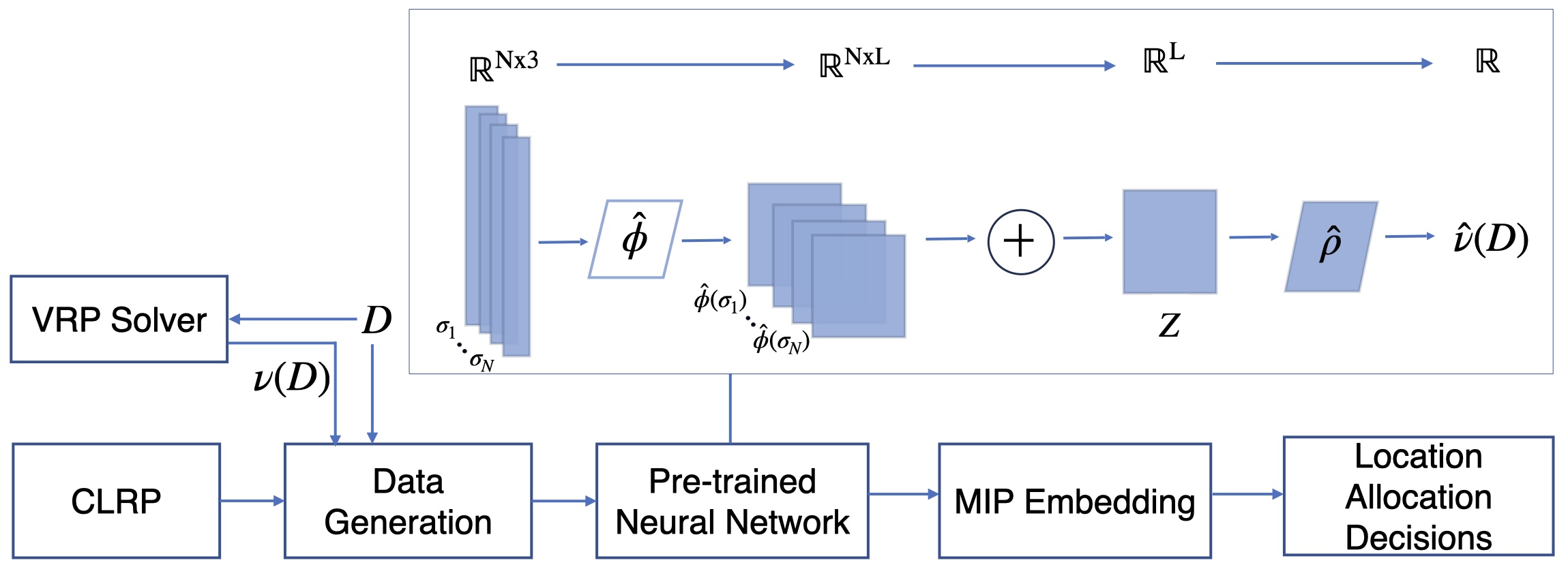
Figure 2: The NEO-LRP framework for solving the CLRP.

In the training phase, NEO-LRP then embeds each individual customer-level feature vector, $\sigma_{j}$, into some $L$-dimensional latent space. This is done by passing each individual feature vector independently through the feature extractor network $\hat{\phi}$, and then aggregating the resulting $|S|$ (denoted as $N$ in Figure 2) latent space features, to produce a single aggregated latent vector $Z$ . This final embedding is then passed through a ReLU feedforward network $\hat{\rho}$ to predict normalized output. In our implementation, $\hat{\phi}$ consists of ReLU-activated layers except for the linear output layer, while $\hat{\rho}$ is entirely composed of ReLU-activated layers including the final output layer.

A key advantage of the architecture is that it can be used to process customer sets $S$ of arbitrary size beyond those that may have been seen during training. Moreover, the feature extractor network $\hat{\phi}$, can be quite complex and does not even have to be ReLU-activated as only the regressor network $\hat{\rho}$ is embedded in the MIP model. This embedding is described in the next section.

4.3 MIP Representation of Neural Surrogate

The MIP model for the neural embedded CLRP can be described as follows.

$$\mathop{\mathrm{minimize}}_{x,y,\gamma,\theta}\;\;\, \sum_{i\in I}\left(f_{i}y_{i}+\gamma_{i}\right)$$ (6)

$$\mathrm{subject\ to}\;\; (x,y)\in X,$$

$$\theta_{il}=\sum_{j\in J}\hat{\phi}_{l}(s_{ij})x_{ij} \forall l\in[L],\;\;i\in I,$$ (7)

$$y_{i}=0\implies\gamma_{i}=0 \;\;\forall i\in I,$$ (8)

$$y_{i}=1\implies\gamma_{i}=\hat{\rho}(\theta_{i1},\dots,\theta_{iL}) \;\;\forall i\in I.$$ (9)

Constraints (7) define the input layer based on Theorem 1. Specifically, $\hat{\phi}_{l}(s_{ij})$ is the $l^{\text{th}}$ component of the $L$-dimensional latent embedding of the feature vector of the customer $j\in J$ normalized with respect to the depot $i\in I$. These latent vectors are pre-computed prior to building the model. The normalized feature vectors $s_{ij}$ and the latent dimension $L$ are also defined in Theorem 1. Constraints (8)–(9) enforce the output of the neural network in the objective function only if depot $i\in I$ is opened and ignore the corresponding output otherwise. These indicator constraints can be reformulated as linear constraints using big-M constants [10]. The right-hand side of the implication constraint (9), namely $\gamma_{i}=\hat{\rho}(\theta_{i1},\dots,\theta_{iL})$, is a neural network constraint. Since $\hat{\rho}$ is a trained feedforward ReLU network, this constraint can be equivalently represented as mixed-integer linear constraints [25]. A complete MIP formulation of the neural embedded CLRP, including an explicit representation of the neural network constraints, can be found in Appendix A.

The embedded MIP model introduces $|I|n$ new binary variables in addition to the location-allocation decisions from (4), where $n$ is the number of hidden units in the trained $\hat{\rho}$ network. Although this number may seem large, our empirical findings indicate that the architecture of the $\hat{\rho}$ neural network can be controlled to make the resulting model easier to solve than traditional MIP-based methods for the CLRP. Specifically, if $K$ is the number of hidden layers and $n_{k}$ is the number of ReLU-activated units in layer $k$, then $n=\sum_{k=1}^{K}n_{k}$. The computational complexity of the MIP can then be directly managed by tuning $K$ and $n_{k}$ during hyperparameter optimization.

4.3.1 Addition of Constraints

A key advantage of the MIP representation is its ability to seamlessly incorporate additional constraints. This flexibility allows the model to handle practical considerations that may be otherwise challenging to address using traditional heuristics designed to optimize over trained neural networks [54, 59]. Below, we briefly describe two examples of constraints that are straightforward to accommodate within the NEO-LRP framework, but may be difficult to handle within traditional heuristics, entailing adjustments and careful enforcement during solution construction or repair.

Incompatibility Constraints Between Customers.

Specific incompatibility or service requirements can prevent certain pairs of customers from being served by the same depot. If $\mathcal{C}\subseteq J\times J$ denotes the set of conflicting customer pairs, then the following constraint can ensure that the customers $j$ and $j^{\prime}$ in $\mathcal{C}$ are not both assigned to the same depot.

$$x_{ij}+x_{ij^{\prime}}\leq 1,\quad\forall(j,j^{\prime})\in\mathcal{C},\;\forall i\in I.$$ (10)

Depot-Specific Assignment Constraints.

Specific customers may only be served by a subset of depots due to operational constraints or agreements. For example, the following constraint can enforce this restriction,

$$x_{ij}=0,\quad\forall i\in I\setminus I_{j},\;j\in J,$$ (11)

where $I_{j}\subseteq I$ is the set of depots allowed to serve customer $j$. This ensures that customer $j$ is assigned only to permissible depots.

4.3.2 Obtaining the Final Routes

The NEO-LRP model (3)–(5) only focuses on determining location-allocation decisions, namely identifying which depots to open (indicated by $y_{i}$), and deciding which customers to assign to these depots (indicated by $x_{ij}$). The neural network surrogate, $\hat{g}_{i}$, approximates the routing cost for assigning a certain subset of customers to depot $i\in I$, thus enabling the MIP solver to efficiently explore the solution space without explicitly calculating any vehicle routes during the solution process. The actual vehicle routes (and true routing costs) can be calculated a posteriori after obtaining a solution of the neural embedded MIP model (6)–(9) and obtaining the location-allocation decisions $(\hat{x},\hat{y})$. Specifically, we extract the subset of customers assigned to each depot $i\in I$, namely $J_{i}(\hat{x})=\{j\in J:\hat{x}_{ij}=1\}$, and then solve the corresponding VRP instance for that depot using an exact VRP solver to determine the true routing cost, $g_{i}(J_{i}(\hat{x}))$, and the optimal vehicle routes associated with that depot. This allows us to calculate the complete CLRP solution and its total cost based on the location-allocation decision obtained by NEO-LRP.

4.4 Data Generation and Model Training

A guiding principle in our data generation procedure is to enable the use of a single pre-trained model that can generalize to input data $D$ of varying numbers of customers and across different depots. To that end, we develop a dataset of input-output pairs $(D,\nu(D))$ by exploring three sampling schemes: Generic VRP Sampling (GVS), Random Subsampling under Capacity Constraints (RSCC), and Proximity-Based Subsampling under Capacity Constraints (PSCC).

• In GVS, we generate VRP instances following the methodology proposed in [58, 49]. The number of customers $N$ is varied in the range $\{1,2,\ldots,100\}$. Similarly, we vary depot positions (random, centered, cornered), customer positions (random, clustered, random-clustered), demand types (various distributions), and average route sizes (from very short to ultra-long) to create a wide range of VRP instances that capture different spatial distributions and demand patterns. We refer the reader to [58, 49] for details. We emphasize that the VRP instances generated using GVS are completely independent of the given CLRP instance and of any distribution from which the given instance may have been drawn.

• In RSCC, we generate VRP instances by subsampling a depot and customer subsets from a given benchmark dataset of CLRP instances. In doing so, we ensure that the total customer demand in each subset does not exceed the capacity of the selected depot. In summary, given a CLRP instance, we randomly select a subset $S\subseteq J$ of customers, such that $|S|=N$ and $N$ is drawn uniformly from $\{1,2,\dots,|J|\}$. A depot $i\in I$ is then selected uniformly at random. We compute the total demand $d_{\mathrm{total}}=\sum_{j\in S}d_{j}$ and check if the capacity constraint $d_{\text{total}}\leq C_{i}$ is satisfied and create a VRP instance with customer set $S$ and depot $i$ if that happens to be the case. A detailed description of the method is given in Appendix B.

• The PSCC method builds upon RSCC by incorporating spatial proximity between depots and customers while still subsampling from the benchmark dataset of CLRP instances. Starting with a CLRP instance, we randomly select a subset $S\subseteq J$ of customers, such that $|S|=N$ and $N$ is drawn uniformly from $\{1,2,\dots,|J|\}$. After computing the total demand $d_{\text{total}}=\sum_{j\in S}d_{j}$, we identify the set of feasible depots $I^{\prime}=\{i\in I:d_{\text{total}}\leq C_{i}\}$. We then select the feasible depot $i^{*}=\arg\min_{i\in I^{\prime}}\sum_{j\in S}c_{ij}$ that minimizes the total distance to the customers in $S$, and form a VRP instance with customer set $S$ and depot $i^{*}$. A detailed description of the method is given in Appendix B.

Each sampling strategy can generate a comprehensive dataset covering various scenarios in terms of customer distribution, demand patterns, and depot assignments. Each VRP instance $D$ in the dataset is solved using an exact or heuristic VRP solver to obtain the label $\nu(D)$, representing its vehicle routing cost. The dataset is finally split into training, validation, and testing sets.

We note that the generated dataset can be quite heterogeneous in terms of the number of customers $N$ in each VRP instance. However, as mentioned in Section 4.1, our neural architecture model naturally allows the processing of inputs of arbitrary size. In actual implementation, this is achieved by first identifying the largest-sized VRP instance across the entire dataset, say with $N_{\max}$ customers. The customer-level features of every other instance are then uniformly padded to have the same length as $N_{\max}$. This allows batch-transformation of this variable-sized dataset via $\hat{\phi}$ into appropriate latent vectors.

4.5 Sparsity Control, Hyperparameter Optimization and Loss Function

The MIP model in Section 4.3 introduces $|I|$ binary variables for each neuron in the regressor network $\hat{\rho}$. Therefore, it is important to explicitly control the number of neurons in the $\hat{\rho}$ network. Although this can be achieved using sparsity control methods such as pruning, we used the strategy of simply restricting the neural network to just one hidden layer. Moreover, as the input of the $\hat{\rho}$ network is equal to the latent dimension $L$, we also explicitly controlled $L$ during hyperparameter optimization. In contrast, the $\hat{\phi}$ network can be quite complex and can have multiple hidden layers. During hyperparameter optimization, 50 random configurations of the neural architecture are evaluated to identify the best network configuration. The range of hyperparameters used is given in Appendix C. We employ mean squared error (MSE) loss for training.

5 Experimental Results and Discussion

All experiments were conducted with an Intel Xeon CPU 6226R and Nvidia Tesla P100-PCIE-12GB GPU, which was primarily utilized for training. We use Gurobi 10.0.3 [29] as the MIP solver, the Gurobi machine learning package [28] for implementing neural network constraints, and Pytorch 2.1.0 [42] for supervised learning tasks. For generating the labels in our dataset, we use the heuristic VRP solver provided by OR-Tools [26] (except in Section 5.5.3). For computing the actual vehicle routes a posteriori as described in Section 4.3.2, we use VRPSolverEasy [22], an exact branch-price-and-cut solver. Our codes, including pre-trained models, are available at https://github.com/Subramanyam-Lab/NEO-LRP.

5.1 Benchmark Instances

The CLRP benchmarks from [44], commonly known as the Prodhon set of instances, are used for the computations. This benchmark set consists of 30 instances ranging in size from 20 customers and 5 depots to 200 customers and 10 depots. All the instances have vehicle capacities of either 70 or 150. The instances are also constrained in terms of depot capacities, and the benchmark set comprises clustered instances as well as those with randomly distributed customers.

5.2 Baselines

We evaluated the performance of our proposed method, NEO-LRP, by comparing it in terms of objective value and computation time against two baselines. The first baseline is a recently proposed state-of-the-art heuristic specifically designed for the CLRP, known as GRASP/VNS [36]. This tailored heuristic combines a Greedy Randomized Adaptive Search Procedure (GRASP) with Variable Neighborhood Search (VNS) to determine the optimal depot locations and associated vehicle routes, considering both depot and vehicle capacities. Unlike GRASP/VNS, our NEO-LRP framework focuses on generating optimal location-allocation decisions without explicitly providing the detailed vehicle routes. NEO-LRP determines which depots to open and assigns customers to these depots, effectively solving only the location-allocation aspects of the problem. The actual vehicle routes are determined a posteriori using an exact VRP Solver [22] We also compared NEO-LRP against a classical model, denoted FLP-VRP. The model is identical to our CLRP formulation given by equations (5)–(4), except for a modification in the objective function. Specifically, the objective function of the FLP model is simplified to account only for the fixed depot opening costs and the direct transportation costs from depots to customers, without considering the vehicle routing costs and constraints. The modified objective function used by FLP-VRP is $h(x,y)=\sum_{i\in I}f_{i}y_{i}+\sum_{i\in I}\sum_{j\in J}c_{ij}x_{ij}$. The final routes are calculated using the procedure described in Section 4.3.2.

5.3 Evaluation Metrics

Optimization Gap with respect to Best Known Solution.

This metric quantifies the relative difference in the objective function value between the solution obtained by a given method and the best known solution (BKS). Let $(x,y)$ denote a candidate solution and let $(x^{*},y^{*})$ denote the reference (possibly optimal) BKS. Then, this metric is defined as:

$$E^{\text{gap}}_{\text{BKS}}=\frac{\left|h(x,y)-h(x^{*},y^{*})\right|}{h(x^{*},y^{*})}$$

Here, $h(x,y)$ is the true objective function given in (5).

Prediction Error of Neural Network.

This metric measures the accuracy of the neural network in approximating the functions $g_{i}$ for all depots $i\in I$ at the solution $(\hat{x},\hat{y})$ determined by NEO-LRP. It is defined as the relative error in the actual and predicted cost over all depots:

$$E^{\text{pred}}=\dfrac{\left|\sum_{i\in I}g_{i}(J_{i}(\hat{x}))-\sum_{i\in I}\hat{g}_{i}(J_{i}(\hat{x}))\hat{y}_{i}\right|}{\sum_{i\in I}g_{i}(J_{i}(\hat{x}))}$$

Mean Absolute Percentage Error on Training and Testing Data.

To evaluate the regression performance of our neural network surrogate model during training and testing, we also compute the Mean Absolute Percentage Error (MAPE) over the respective datasets.

5.4 Comparison with Baselines

In this section, we compare the results of NEO-LRP with GRASP/VNS and FLP-VRP, across the instances in the benchmark set consisting of 20, 50, 100 and 200 customers. Table 1 lists each instance and its corresponding best known solution (BKS) taken from [36]. Since NEO-LRP incorporates supervised machine learning, it incurs a one-time computational cost for data generation and neural network training. For comparisons with baseline methods, we generated 10,000 unique VRP instances across all 30 CLRP instances using the RSCC data sampling method. These samples were divided into training and validation sets with a 90-10 split, we also sample 10,000 more instances for testing purposes. Data sampling took approximately $T_{\text{sampling}}=3\text{ min}$, due to parallelization over $400$ CPU cores. Solving the 20,000 VRP instances using the heuristic solver with a 30-second time limit per instance required a total of approximately $T_{\text{solving}}=25$ min. Neural network training, including hyperparameter optimization over 61 evaluations with 10 parallel workers on 1 GPU, took $T_{\text{training}}=1.6\text{ hours}$. Testing time was $T_{\text{testing}}=14\text{ sec}$. The total computational time was approximately $T_{\text{one-time}}=2.1$ wall-clock hours. Once trained, the neural network models $\hat{\phi}$ and $\hat{\rho}$ can be utilized out-of-the-box without incurring any additional costs.

In the case of NEO-LRP and FLP-VRP, we first determine the optimal location-allocation decisions by solving their respective MIP models. As described in Section 4.3.2, we then compute the actual vehicle routes a posteriori using an exact VRP solver [22] to obtain the true routing costs, ensuring that the final objective values reflect the true transportation costs. We calculate the gap between the total cost of the best solution obtained using this approach and the BKS, which is then reported in the respective columns titled $E^{\text{gap}}_{\text{BKS}}$. For each of these methods, we report both the time required for location-allocation decisions ($T_{\text{LA}}$) and the total computational time including routing ($T_{\text{total}}$), where both gaps and times are averaged over five runs. In contrast, GRASP/VNS simultaneously determines both location and routing decisions. We take the total computational times ($T_{\text{total}}$) and solution gaps as reported in [36], which are also averaged over five runs. We note that the computation times of GRASP/VNS were obtained using an Intel Xeon E5 processor, and may not be directly comparable with those of NEO-LRP and FLP.

Table 1: Performance versus baselines on all benchmarks instances (averaged over five runs).

		NEO-LRP			FLP-VRP			GRASP/VNS
Instance	BKS	$E^{\text{gap}}_{\text{BKS}}$(%)	$T_{\text{LA}}$ (s)	$T_{\text{total}}$ (s)	$E^{\text{gap}}_{\text{BKS}}$(%)	$T_{\text{LA}}$ (s)	$T_{\text{total}}$ (s)	$E^{\text{gap}}_{\text{BKS}}$(%)	$T_{\text{total}}$ (s)
20-5-1a	54,793	3.24	0.24	0.40	4.38	0.03	0.22	0.08	0.78
20-5-1b	39,104	3.65	0.22	0.27	6.30	0.01	0.07	0.00	0.67
20-5-2a	48,908	3.22	0.26	0.39	0.58	0.10	0.16	0.00	0.76
20-5-2b	37,542	7.16	0.17	0.27	14.59	0.06	0.12	0.00	0.65
Average		4.32	0.22	0.33	6.46	0.05	0.14	0.02	0.71
50-5-1a	90,111	1.63	0.24	1.05	2.94	0.01	0.22	0.00	7.95
50-5-1b	63,242	3.83	0.17	2.07	11.66	0.01	0.93	0.00	8.59
50-5-2a	88,293	3.98	0.56	1.80	4.50	0.77	1.33	0.35	8.52
50-5-2b	67,308	5.68	0.49	1.21	7.46	0.77	2.10	0.54	9.18
50-5-2bbis	51,822	3.76	0.67	0.96	3.92	0.23	1.58	0.02	8.98
50-5-2bis	84,055	1.47	0.50	1.36	1.47	0.13	0.94	0.00	7.90
50-5-3a	86,203	2.82	0.27	3.42	10.48	0.05	1.05	0.19	7.78
50-5-3b	61,830	6.25	0.48	1.43	24.08	0.05	0.30	0.00	7.59
Average		3.68	0.42	1.66	8.31	0.26	1.06	0.14	8.31
100-5-1a	274,814	1.41	1.39	17.86	1.28	1.11	13.21	0.44	70.15
100-5-1b	213,568	1.25	2.19	43.58	1.22	1.12	7.13	0.38	70.81
100-5-2a	193,671	0.43	0.22	8.13	0.43	0.08	6.16	0.23	82.00
100-5-2b	157,095	0.73	0.30	52.20	0.73	0.08	53.74	0.07	61.93
100-5-3a	200,079	1.48	0.70	19.81	0.76	0.48	3.20	0.24	64.37
100-5-3b	152,441	2.26	0.56	34.64	2.08	0.49	12.43	1.03	57.29
100-10-1a	287,661	3.81	3.15	20.84	2.48	11.74	22.39	0.61	78.81
100-10-1b	230,989	3.23	2.74	6.24	5.13	11.76	14.41	1.19	87.95
100-10-2a	243,590	1.68	1.92	17.26	1.84	2.23	6.95	2.06	75.65
100-10-2b	203,988	2.12	2.93	6.71	2.52	2.25	6.55	1.23	67.50
100-10-3a	250,882	0.98	1.52	13.13	0.98	8.91	13.27	3.83	71.87
100-10-3b	203,114	1.83	1.60	10.10	2.13	8.93	21.31	5.53	79.76
Average		1.77	1.60	20.88	1.80	4.10	15.06	1.40	72.34
200-10-1a	474,850	0.83	3.51	63.34	1.95	3.51	143.22	3.16	752.03
200-10-1b	375,177	0.56	4.16	963.63	2.87	3.51	68.41	2.74	735.75
200-10-2a	448,077	0.47	3.39	682.98	0.34	0.48	130.44	0.38	642.16
200-10-2b	373,696	0.30	2.91	98.69	0.30	0.48	49.01	0.23	683.19
200-10-3a	469,433	0.80	3.04	57.17	0.90	1.14	29.47	0.48	661.82
200-10-3b	362,320	1.85	4.10	722.45	6.12	1.15	374.98	0.45	818.25
Average		0.80	3.52	431.38	2.08	1.71	132.59	1.24	715.53

Table 1 shows that, despite their simplicity, both NEO-LRP and FLP-VRP provide location-allocation decisions that are on average within 5% of the BKS across all instances. Specifically, NEO-LRP achieves an average gap of 4.32% for the 20-customer instances, 3.68% for the 50-customer instances, 1.77% for the 100-customer instances and 0.80% for the 200-customer instances. This demonstrates a consistent improvement in solution quality as the problem size increases, hinting that our single pre-trained model may perform better on the larger instances.

Table 1 also highlights significant trade-offs between solution quality and computational time. GRASP/VNS achieves the smallest average gaps across all instance sizes (e.g., 0.14% for the 50-customer instances and 1.40% for the 100-customer instances), except for the 200-customer instances where NEO-LRP achieves a better gap of 0.80% compared to GRASP/VNS’s 1.24%. In terms of computational efficiency, NEO-LRP is consistently faster than GRASP/VNS, being 3.5 times faster for 100-customer instances and 1.7 times faster for 200-customer instances. Most notably, NEO-LRP can obtain high-quality location-allocation decisions extremely quickly, requiring only 1.6 seconds on average for 100-customer instances and 3.5 seconds for 200-customer instances, not including the routing phase.

Although FLP-VRP provides results close to NEO-LRP in terms of solution quality for smaller instances, its performance becomes less competitive as the instance size grows, with higher computational times particularly for larger instances. The trade-offs between solution quality and computational time vary significantly with problem size. For small instances (20-50 customers), GRASP/VNS clearly dominates with near-optimal solutions (gaps of 0.02% and 0.14% respectively) with minimal time. For medium-sized instances (100 customers), GRASP/VNS achieves slightly better solutions (1.40% gap) but at significantly higher computational cost, while for large instances (200 customers), NEO-LRP dominates in both solution quality (0.80% gap versus 1.24%) and computational efficiency. Overall, NEO-LRP emerges as a particularly effective method for large-scale problems, striking a good balance between solution quality and computational efficiency.

5.5 Ablation Studies

We perform detailed experimental analyses to understand the impact of various components of our framework, including the choice of sampling method, sample requirements for training, choice of vehicle routing solvers for generating labeled training data, as well as the use of single pre-trained versus instance-specific neural surrogates. All results are averaged over 5 runs.

5.5.1 Effect of Different Sampling Methods

For each sampling method–Generic VRP Sampling (GVS), Random Subsampling under Capacity Constraints (RSCC), and Proximity-based Subsampling under Capacity Constraints (PSCC)–we generate 10,000 VRP instances. Of these, 90% are used for training, while the remaining 10% are used for validation during hyperparameter optimization. In addition, a separate test set of 10,000 unique VRP instances is sampled to evaluate the trained network. We solve each VRP instance $D$ using a heuristic routing solver [26] with a 30-second time limit to compute the label $\nu(D)$.

We observe that the neural networks $\hat{\phi}$ and $\hat{\rho}$ trained using the RSCC sampling method achieve the lowest median gap $E^{\text{gap}}_{\text{BKS}}$ of 1.84%, compared to GVS at 4.29% and PSCC at 2.79%. To further understand the performance, we analyze how each sampling method influences the prediction error $E^{\text{pred}}$ and test error $E^{\text{test}}$, and their relationship with the total transportation cost.

Recall that the prediction error $E^{\text{pred}}$ measures how well the neural networks approximate the total transportation cost. On the other hand, the test error $E^{\text{test}}$ evaluates the performance of the trained neural networks on test instances sampled using the same method as the training data. These test instances represent subsets of customers but may not fully reflect the actual customer assignments $J_{i}({x})$ that are encountered during optimization. Sampling methods influence the model’s ability to generalize to these optimization assignments.

Figure 3: Comparison of sampling methods on (a) $E^{\text{test}}$, (b) $E^{\text{pred}}$, (c) $E^{\text{gap}}_{\text{BKS}}$

The GVS sampling method generates instances inspired by [58, 49] and aims to create diverse spatial and demand distributions of customer sets $S$. This diversity allows GVS to achieve a relatively low median $E^{\text{test}}$ of 2.87%. However, the median $E^{\text{pred}}$ is much higher at 58.31%, indicating poor generalization to the customer assignments $J_{i}(x)$ encountered during optimization. We believe that this discrepancy arises because, although the training and test instances share the same distribution, the actual assignments $J_{i}(x)$ during optimization may not be representative of this distribution. Therefore, we see that neural networks trained with GVS struggle to accurately approximate $g_{i}(J_{i}(x))$. Similar observations has also been reported previously in [54].

In contrast, the RSCC method directly subsamples random customer subsets $S$ from CLRP instances. We believe that this alignment between the training data and the customer assignments $J_{i}(x)$ during optimization results in a lower median $E^{\text{pred}}$ of 9.64%, which directly translates into the lowest median $E^{\text{gap}}_{\text{BKS}}$ of 1.84%. PSCC is similar to RSCC except that it incorporates spatial proximity constraints, achieving slightly higher median $E^{\text{pred}}$ (12%) and median $E^{\text{gap}}_{\text{BKS}}$ (2.79%). We believe that proximity constraints may reduce the diversity of training samples, limiting the neural network’s ability to generalize compared to RSCC.

Despite the significance of $E^{\text{pred}}$ as a performance indicator, it is important to note that even when $E^{\text{pred}}$ is high the corresponding optimization gap $E^{\text{gap}}_{\text{BKS}}$ remains relatively small (see Figure 3). This can be attributed to the solution selection mechanism in NEO-LRP. While the neural surrogate may have prediction errors it still effectively guides the search toward promising regions of the solution space. NEO-LRP uses the neural surrogate predictions to explore the solution space and computes the true cost by solving the corresponding VRP only for the final best solution. The final verification approach means that although the neural surrogate predictions may have errors (as shown by $E^{\text{pred}}$ particularly for GVS) it is still capable of identifying high-quality solutions when evaluated exactly as measured by $E^{\text{gap}}_{\text{BKS}}$. The neural surrogate effectively guides the search for feasible solutions while the exact computation of transportation costs for the best identified solution enables accurate final evaluation. Consequently, a high $E^{\text{pred}}$ does not adversely affect the optimization gap $E^{\text{gap}}_{\text{BKS}}$ as one might expect.

5.5.2 Effect of Sample Size

We study the effect of sample size on the performance of NEO-LRP by varying the number of VRP instances used to train the neural networks $\hat{\phi}$ and $\hat{\rho}$. The RSCC sampling method is used to generate training and validation datasets of sizes 100, 1000, 10,000, 100,000, while keeping the test set fixed at 10,000 instances. We use a heuristic solver [26] to compute the true labels. The data is split into training and validation sets using a 90-10 split. We then train neural networks and solve the embedded model and finally evaluate the solutions using the metrics $E^{\text{gap}}_{\text{BKS}}$, $E^{\text{pred}}$, and $E^{\text{test}}$.

The results are summarized in Figure 4. We observe that as the training sample size $N_{train}$ increases, both the test error $E^{\text{test}}$ and the prediction error $E^{\text{pred}}$ decrease, indicating improved neural network performance on unseen data. Specifically, the median $E^{\text{test}}$ decreases from 11.37% to 3.74%, and median $E^{\text{pred}}$ decreases from 12.11% to 7.40% when $N_{train}$ increases from 100 to 100,000. However, the median $E^{\text{gap}}_{\text{BKS}}$ remains relatively constant across different sample sizes, fluctuating only slightly around 1.77%. This observation suggests that increasing the training sample size has a limited effect on the final solution quality in terms of the optimization gap $E^{\text{gap}}_{\text{BKS}}$. The decrease in $E^{\text{test}}$ and $E^{\text{pred}}$ with larger training datasets is expected, as more data enables the neural networks to learn better representations and generalize effectively to unseen instances.

Figure 4: Effect of sample size on (a) $E^{\text{test}}$, (b) $E^{\text{pred}}$, (c) $E^{\text{gap}}_{\text{BKS}}$.

5.5.3 Effect of Routing Solver

We study the effect of the solver used to generate the target label and its effect on $E^{\text{gap}}_{\text{BKS}}$. To examine this, we use the RSCC method to generate a total of 10,000 VRP training and validation instances along with a separate test set of 10,000 instances. If we denote the target label generated by a heuristic solver as $\nu^{\text{heuristic}}(D)$, and the target label generated by an exact solver as $\nu^{\text{exact}}(D)$. Each VRP instance is solved using a heuristic solver [26] with a time limit of 30 seconds to compute $\nu^{\text{heuristic}}(D)$ and an exact solver [22] with a time limit of 1800 seconds to compute $\nu^{\text{exact}}(D)$. To quantify the difference between these two solvers, we define the label gap ($E^{\text{label}}$) as the percentage discrepancy between the heuristic and exact solvers for the same VRP instance $D$ as follows:

$$E^{\text{label}}=\frac{|\nu^{\text{exact}}(D)-\nu^{\text{heuristic}}(D)|}{\nu^{\text{exact}}(D)}\times 100\%.$$

After solving the 20,000 VRP instances (training, validation, and test), we observe that $E^{\text{label}}$ remained below 5% for more than 99% of the instances, with only four instances exceeding 5% (see Figure 5). We found that the exact solver was efficient, taking an average of 6.29 seconds to solve each instance, though with a standard deviation of 62.58 seconds. In contrast, the heuristic solver required an average of 29.3 seconds per instance with a lower standard deviation of 4.53 seconds. The total time required by the exact solver was less than that of the heuristic solver. We also observe that the choice of solver had a minimal effect on the time required to train the neural network. The model trained using heuristically generated labels completed training in 1.6 hours, whereas the model using exactly generated labels $\nu^{\text{exact}}(D)$ required only slightly longer time at 1.8 hours.

We observe that the solver choice has minimal impact on the framework’s performance in terms of $E^{\text{gap}}_{\text{BKS}}$. Using exact label generation, NEO-LRP achieves a median $E^{\text{gap}}_{\text{BKS}}$ of 1.24%, whereas median $E^{\text{gap}}_{\text{BKS}}$ is 1.84% when we use heuristic solvers. Our findings suggest that while both approaches are viable, we recommend using the exact solver for VRP instances with fewer customers, whereas the heuristic solver may be more appropriate for handling larger instances.

Figure 5: Comparison of exact versus heuristic VRP solvers: (a) Solver time (s) , (b) $E^{\text{gap}}_{\text{BKS}}$, (c) Histogram of $E^{\text{label}}$(%) across 0–5% (as only 4 instances exceed 5%).

5.5.4 Effect of Problem Size

We examine the effect of problem size on the performance of NEO-LRP, considering problem sizes with 20, 50, 100, and 200 customers. Using each of the sampling methods (GVS, RSCC, and PSCC), we generate a total of 10,000 VRP instances, which are then split into training and testing sets with a 90-10 split. Three separate neural networks are trained on the heterogeneous dataset generated by each sampling method. Each model is then embedded within the optimization framework and solved using off-the-shelf solver [29]. The results are presented in Figure 6.

We observe that as the problem size increases $E^{\text{gap}}_{\text{BKS}}$ decreases for all three sampling methods. This indicates that, regardless of the sampling method, the trained neural networks perform better as the problem size grows. This trend suggests that the NEO-LRP framework is capable of performing better with larger problem instances, even though the models are trained on a small fixed heterogenous dataset of 10,000 instances. The observed reduction in $E^{\text{gap}}_{\text{BKS}}$ as the problem size increases supports our hypothesis that a single neural network, when trained on a sufficiently diverse dataset, performs better on larger problem instances. This behavior is consistent across all three sampling methods, with each benefiting from the larger problem sizes. Our results demonstrate NEO-LRP’s ability to identify high-quality solutions improves as the size of instances increases.

Figure 6: Effect of problem size (the $x$-axis represents the number of customers in the instance).

5.5.5 Single versus Customized Neural Networks

We study the effect of using a single neural network trained on a heterogeneous dataset across all benchmark instances compared to using customized neural networks for each specific instance.

Single Neural Network.

We sample 10,000 VRP instances using RSCC across all the benchmark instances and train a single neural network on this dataset. Each neural network is trained on a 90-10 split of the sampled instances.

Customized Neural Networks.

For each of the individual benchmark instances, we sample 10,000 instances specifically for that problem and train a unique neural network for each benchmark instance. This results in 30 distinct pairs of $\hat{\phi}$ and $\hat{\rho}$ respectively, one for each of the 30 benchmark instances. Each neural network is trained on a 90-10 split of the sampled instances.

The results are presented in Table 2. Perhaps counterintuitively, we observe that using a single neural network provides comparable, and in some cases better, performance than using customized neural networks. For the 20-customer instances, the average optimization gap $E^{\text{gap}}_{\text{BKS}}$ is 4.32% for the single neural network and 3.27% for the customized networks. For the 50-customer instances, the single neural network achieves an average gap of 3.68%, while the customized networks have a slightly better average of 3.14%. For the 100-customer instances, the single neural network achieves an average gap of 1.77%, while the customized networks have a comparable average of 1.54%. However, for larger instances with 200 customers, the single neural network outperforms the customized networks. Specifically, for the 200-customer instances, the average optimization gap is 0.80% with the single network compared to 1.21% with customized networks.

Table 2: Results comparing the effect of single vs customized neural networks

		Single			Customized
Instance	BKS	$E^{\mathrm{gap}}_{\mathrm{BKS}}$	$T_{\mathrm{LA}}$	$T_{\mathrm{total}}$	$E^{\mathrm{gap}}_{\mathrm{BKS}}$	$T_{\mathrm{LA}}$	$T_{\mathrm{total}}$
20-5-1a	54,793	3.24	0.24	0.40	3.24	0.27	0.40
20-5-1b	39,104	3.65	0.22	0.27	6.48	3.63	3.71
20-5-2a	48,908	3.22	0.26	0.39	3.22	0.19	0.31
20-5-2b	37,542	7.16	0.17	0.27	0.13	3.89	3.97
Average		4.32	0.22	0.33	3.27	1.99	2.10
50-5-1a	90,111	1.63	0.24	1.05	0.26	0.20	0.41
50-5-1b	63,242	3.83	0.17	2.07	1.18	0.44	6.01
50-5-2a	88,293	3.98	0.56	1.80	4.50	0.13	1.08
50-5-2b	67,308	5.68	0.49	1.21	5.17	0.27	1.70
50-5-2bbis	51,822	3.76	0.67	0.96	4.79	0.41	1.66
50-5-2bis	84,055	1.47	0.50	1.36	2.67	0.46	1.30
50-5-3a	86,203	2.82	0.27	3.42	1.43	0.26	0.93
50-5-3b	61,830	6.25	0.48	1.43	5.10	0.59	1.19
Average		3.68	0.42	1.66	3.14	0.35	1.78
100-5-1a	274,814	1.41	1.39	17.86	1.25	1.99	11.20
100-5-1b	213,568	1.25	2.19	43.58	1.38	0.98	12.74
100-5-2a	193,671	0.43	0.22	8.13	0.43	0.62	7.75
100-5-2b	157,095	0.73	0.30	52.20	0.73	0.51	49.20
100-5-3a	200,079	1.48	0.70	19.81	1.07	0.74	9.21
100-5-3b	152,441	2.26	0.56	34.64	0.71	2.42	5.57
100-10-1a	287,661	3.81	3.15	20.84	2.16	24.25	35.32
100-10-1b	230,989	3.23	2.74	6.24	4.64	40.32	45.26
100-10-2a	243,590	1.68	1.92	17.26	1.15	8.98	20.02
100-10-2b	203,988	2.12	2.93	6.71	2.22	11.39	13.45
100-10-3a	250,882	0.98	1.52	13.13	0.61	10.81	21.02
100-10-3b	203,114	1.83	1.60	10.10	2.13	2.84	24.28
Average		1.77	1.60	20.88	1.54	8.82	21.25
200-10-1a	474,850	0.83	3.51	63.34	1.74	27.52	774.19
200-10-1b	375,177	0.56	4.16	963.63	0.93	17.15	71.63
200-10-2a	448,077	0.47	3.39	682.98	0.26	5.67	640.65
200-10-2b	373,696	0.30	2.91	98.69	0.66	22.16	88.44
200-10-3a	469,433	0.80	3.04	57.17	0.96	16.53	339.41
200-10-3b	362, 320	1.85	4.10	722.45	2.72	15.85	36.60
Average		0.80	3.52	431.38	1.21	17.48	325.15

In terms of computation time, the single neural network consistently requires less $T_{\text{LA}}$ than the customized networks across all instance sizes. This difference becomes more pronounced as the problem size increases. For the 100-customer instances, the single network requires only 1.60 seconds compared to 8.82 seconds for customized networks, and for 200-customer instances, the difference is even more substantial (3.52 seconds versus 17.48 seconds). When considering the total computational time including routing ($T_{\text{total}}$), both approaches show comparable performance. For 100-customer instances, both methods require similar time (20.88 seconds versus 21.25 seconds), while for 200-customer instances, the total times are 431.38 seconds and 325.15 seconds respectively. This suggests that while the single network is significantly more efficient in making location-allocation decisions, the routing phase dominates the overall computational effort, resulting in comparable total solution times between the approaches.

However, the training time for the neural networks differs significantly between the two approaches. Training the single neural network on one GPU with 10 workers took approximately 1.6 hours. In contrast, training all 30 customized neural networks took a total of 35.5 hours, utilizing 2 GPUs and 10 workers. This highlights a substantial reduction in training time when using a single neural network.

These results highlight several key insights. First, a single neural network trained on a diverse dataset generalizes well across different problem instances, even outperforming instance-specific models for larger problems. This suggests that NEO-LRP’s neural surrogate effectively captures the underlying structure of the problem and enables it to make better predictions across a variety of instances. Second, the use of a single neural network significantly reduces computational overhead and makes the approach more scalable and practical. We observe that the NEO-LRP framework demonstrates strong generalization capabilities with a single pre-trained neural network achieving high-quality solutions with lower computational effort compared to customized neural networks.

6 Conclusion

Our paper offers a fresh approach to combine machine learning with integer programming to solve location-routing problems. The proposed model, NEO-LRP, is a generic solution framework that first approximates the (difficult-to-compute) vehicle routing cost associated with each open facility using a sparse neural surrogate and then embeds this surrogate into an easy-to-solve MIP model. A key benefit of our model is that it can avoid potentially costly, time consuming, and complex implementations that are typical of the state-of-the-art heuristics while also being able to generalize to problems with other types of side constraints. Our experiments showed that NEO-LRP can achieve high-quality solutions quickly, especially for larger instances. In terms of the future work, our methodology can be extended in several directions. While the current neural network training focuses on minimizing test error, incorporating a ranking-preserving loss function could help identify promising solutions that might be overestimated and prematurely discarded during the neural-embedded optimization. This approach would ensure the correct ordering of solution costs even when absolute predictions are not highly accurate. Another promising direction is to investigate the potential of the method in addressing other applications, involving integrated planning and scheduling decisions.

7 Acknowledgments

We acknowledge support from the United States Department of Energy, award number DE-SC0023361. Computations for this research were performed on the Pennsylvania State University’s Institute for Computational and Data Sciences’ Roar supercomputer.

Appendix

Appendix A Neural Embedded MIP Formulation

We provide here the complete MIP formulation for the neural embedded CLRP. This model builds upon the formulation originally proposed in [25] for embedding a trained neural network within a MIP. Suppose that the trained $\hat{\rho}$ network contains $K$ hidden layers, numbered $1$ to $K$, and layer $k\in[K]\coloneqq\{1,2,\ldots,K\}$ contains $n_{k}$ ReLU-activated units (i.e., neurons), numbered $1$ to $n_{k}$. For ease of notation, let $k=0$ denote the input layer, so that $n_{0}\coloneqq L$ (the latent dimension from Theorem 1) and $k=K+1$ denote the output layer. Let $w^{k-1}_{\ell m}$ be the weight of the output from neuron $\ell$ in layer $k-1$ that feeds into neuron $m\in[n_{k}]\coloneqq\{1,2,\ldots,n_{k}\}$ in layer $k$, whose bias we denote as $b_{m}^{k}$. For each $i\in I$, we use continuous non-negative variables $\theta_{im}^{k}$ and slack variable $\nu_{im}^{k}$ to encode the output of unit $m$ in layer $k$. The binary variable $z_{im}^{k}$ indicates if the neuron is active; that is, if $\theta_{im}^{k}\geq 0$ and $\nu_{im}^{k}=0$. The complete MIP model can be described as follows:

$$\mathop{\mathrm{minimize}}_{x,y,z,\gamma,\theta,\nu}\;\;\, \sum_{i\in I}\left(f_{i}y_{i}+\gamma_{i}\right)$$ (12)

$$\mathrm{subject\ to}\;\; (x,y)\in X,$$

$$\theta^{0}_{il}=\sum_{j\in J}\hat{\phi}_{l}(s_{ij})x_{ij} \forall l\in[n_{0}],\;\;i\in I,$$ (13)

$$\sum_{\ell=1}^{n_{k-1}}w_{\ell m}^{k-1}\theta^{k-1}_{im}+b_{m}^{k}=\theta_{im}^{k}-\nu_{im}^{k} \forall m\in[n_{k}],\;k\in[K],\;\;i\in I,$$ (14)

$$z_{im}^{k}=1\implies\nu_{im}^{k}=0 \forall m\in[n_{k}],\;k\in[K],\;\;i\in I,$$ (15)

$$z_{im}^{k}=0\implies\theta_{im}^{k}=0 \forall m\in[n_{k}],\;k\in[K],\;\;i\in I,$$ (16)

$$y_{i}=1\implies\gamma_{i}=\sum_{\ell=1}^{n_{K}}w_{\ell m}^{K}\theta^{K}_{im}+b_{m}^{K+1} \forall i\in I,$$ (17)

$$y_{i}=0\implies\gamma_{i}=0 \forall i\in I,$$ (18)

$$z_{im}^{k}\in\{0,1\},\;\theta_{im}^{k}\geq 0,\;\nu_{im}^{k}\geq 0 \forall m\in[n_{k}],\;k\in[K],\;\;i\in I.$$ (19)

Constraints (13) define the input layer based on the embedding from Theorem 1. Constraints (14)–(16) enforce the desired ReLU-activated output from each hidden layer $k$. Constraints (17)–(18) enforce the output of the neural network in the objective function only when depot $i\in I$ is opened, and ignore the corresponding output otherwise. We note that the indicator constraints (15)–(18) can be reformulated as linear constraints [10].

Appendix B Sampling Schemes

Algorithm 1 Random Subsampling under Capacity Constraints (RSCC)

0: Dataset $D_{\text{LRP}}$ of CLRP instances, desired number $N_{\mathrm{data}}$ of VRP instances.

0: Generated dataset of VRP instances, $D_{\text{VRP}}$.

1: Initialize $D_{\text{VRP}}\leftarrow\emptyset$

2: while $|D_{\text{VRP}}|<N_{\text{data}}$ do

3:  Select $\left(I,J,\{C_{i}\}_{i\in I},\{(u_{i}^{0},v_{i}^{0})\}_{i\in I},\{(u_{j},v_{j},d_{j})\}_{j\in J},Q,F\right)\in D_{\text{LRP}}$ uniformly at random

4:  Choose $N\in\{1,2,\dots,|J|\}$ uniformly at random

5:  Sample a subset $S\subseteq J$ with $|S|=N$ uniformly at random

6:  Select a depot $i\in I$ uniformly at random

7:  Compute total demand $d_{\text{total}}=\sum_{j\in S}d_{j}$

8:  if $d_{\text{total}}\leq C_{i}$ then

9:   Define VRP instance $D=\left(u_{i}^{0},v_{i}^{0},\{(u_{j},v_{j},d_{j})\}_{j\in S},Q,F\right)$

10:   if $D\notin D_{\text{VRP}}$ then

11:    $D_{\text{VRP}}\leftarrow D_{\text{VRP}}\cup\{D\}$

12:   end if

13:  end if

14: end while

Algorithm 2 Proximity-Based Subsampling under Capacity Constraints (PSCC)

0: Dataset $D_{\text{LRP}}$ of CLRP instances, desired number $N_{\mathrm{data}}$ of VRP instances.

0: Generated dataset of VRP instances, $D_{\text{VRP}}$.

1: Initialize $D_{\text{VRP}}\leftarrow\emptyset$

2: while $|D_{\text{VRP}}|<N_{\mathrm{data}}$ do

3:  Select $\left(I,J,\{C_{i}\}_{i\in I},\{(u_{i}^{0},v_{i}^{0})\}_{i\in I},\{(u_{j},v_{j},d_{j})\}_{j\in J},Q,F\right)\in D_{\text{LRP}}$ uniformly at random

4:  Choose $N\in\{1,2,\dots,|J|\}$ uniformly at random

5:  Sample a subset $S\subseteq J$ with $|S|=N$ uniformly at random

6:  Compute total demand $d_{\text{total}}=\sum_{j\in S}d_{j}$

7:  Let $I^{\prime}=\{i\in I:d_{\text{total}}\leq C_{i}\}$

8:  if  $I^{\prime}\neq\emptyset$  then

9:   Select $i^{*}\in\arg\min_{i\in I^{\prime}}\left\{\sum_{j\in S}c_{ij}\right\}$

10:   Define VRP instance $D=\left(u_{i^{*}}^{0},v_{i^{*}}^{0},\{(u_{j},v_{j},d_{j})\}_{j\in S},Q,F\right)$

11:   if $D\notin D_{\text{VRP}}$ then

12:    $D_{\text{VRP}}\leftarrow D_{\text{VRP}}\cup\{D\}$

13:   end if

14:  end if

15: end while

Appendix C Hyperparameters

Table 3: Neural Network Hyperparameters and their Ranges

Hyperparameter	Range
Latent space dimension	{4, 6, 8}
Number of hidden layers in $\hat{\phi}$	{2, 3, 4, 5, 6}
Number of hidden layers in $\hat{\rho}$	{1}
Neurons per layer in $\hat{\phi}$	{32, 64, 128, 256, 512, 1024, 2048}
Neurons per layer in $\hat{\rho}$	{4, 6, 8}
Early stopping patience	{15, 20}
Batch size	{32}
Learning rate	{0.001}
Number of epochs	{50, 100, 200, 400, 600, 800, 1000}
Optimizer	Adam
Loss function	MSE
Activation function	ReLU

References

- [1] Akca, Z., Berger, R., Ralphs, T.: A branch-and-price algorithm for combined location and routing problems under capacity restrictions. In: Operations research and cyber-infrastructure. pp. 309–330. Springer (2009)
- [2] Albareda-Sambola, M., Rodríguez-Pereira, J.: Location-routing and location-arc routing. Location science pp. 431–451 (2019)
- [3] Albareda-Sambola, M., Rodríguez-Pereira, J.: Location-Routing and Location-Arc Routing. In: Laporte, G., Nickel, S., Saldanha-da Gama, F. (eds.) Location Science, pp. 431–451. Springer, Cham, Switzerland, 2 edn. (2020)
- [4] Alvim, A.C., Taillard, É.D.: Popmusic for the world location-routing problem. EURO Journal on Transportation and Logistics 2(3), 231–254 (2013)
- [5] Baldacci, R., Mingozzi, A., Wolfler Calvo, R.: An exact method for the capacitated location-routing problem. Operations research 59(5), 1284–1296 (2011)
- [6] Belenguer, J.M., Benavent, E., Prins, C., Prodhon, C., Calvo, R.W.: A branch-and-cut method for the capacitated location-routing problem. Computers & Operations Research 38(6), 931–941 (2011)
- [7] Bengio, Y., Lodi, A., Prouvost, A.: Machine learning for combinatorial optimization: a methodological tour d’horizon. European Journal of Operational Research 290(2), 405–421 (2021)
- [8] Berger, R.T., Coullard, C.R., Daskin, M.S.: Location-routing problems with distance constraints. Transportation Science 41(1), 29–43 (2007)
- [9] Bogyrbayeva, A., Meraliyev, M., Mustakhov, T., Dauletbayev, B.: Learning to solve vehicle routing problems: A survey. arXiv preprint arXiv:2205.02453 (2022)
- [10] Bonami, P., Lodi, A., Tramontani, A., Wiese, S.: On mathematical programming with indicator constraints. Mathematical programming 151, 191–223 (2015)
- [11] Bouhafs, L., Hajjam, A., Koukam, A.: A combination of simulated annealing and ant colony system for the capacitated location-routing problem. In: Knowledge-Based Intelligent Information and Engineering Systems: 10th International Conference, KES 2006, Bournemouth, UK, October 9-11, 2006. Proceedings, Part I 10. pp. 409–416. Springer (2006)
- [12] Cappart, Q., Chételat, D., Khalil, E.B., Lodi, A., Morris, C., Veličković, P.: Combinatorial optimization and reasoning with graph neural networks. Journal of Machine Learning Research 24(130), 1–61 (2023)
- [13] Ceccon, F., Jalving, J., Haddad, J., Thebelt, A., Tsay, C., Laird, C.D., Misener, R.: Omlt: Optimization & machine learning toolkit. The Journal of Machine Learning Research 23(1), 15829–15836 (2022)
- [14] Chan, Y., Baker, S.F.: The multiple depot, multiple traveling salesmen facility-location problem: Vehicle range, service frequency, and heuristic implementations. Mathematical and Computer Modelling 41(8-9), 1035–1053 (2005)
- [15] Contardo, C., Cordeau, J.F., Gendron, B.: A computational comparison of flow formulations for the capacitated location-routing problem. Discrete Optimization 10(4), 263–295 (2013)
- [16] Contardo, C., Cordeau, J.F., Gendron, B.: An exact algorithm based on cut-and-column generation for the capacitated location-routing problem. INFORMS Journal on Computing 26(1), 88–102 (2014)
- [17] Cuda, R., Guastaroba, G., Speranza, M.G.: A survey on two-echelon routing problems. Computers & Operations Research 55, 185–199 (2015)
- [18] Derbel, H., Jarboui, B., Hanafi, S., Chabchoub, H.: Genetic algorithm with iterated local search for solving a location-routing problem. Expert Systems with Applications 39(3), 2865–2871 (2012)
- [19] Drexl, M., Schneider, M.: A survey of variants and extensions of the location-routing problem. European journal of operational research 241(2), 283–308 (2015)
- [20] Duhamel, C., Lacomme, P., Prins, C., Prodhon, C.: A memetic approach for the capacitated location routing problem. In: Proceedings of the 9th EU/Meeting on Metaheuristics for Logistics and Vehicle Routing, Troyes, France. vol. 38, p. 39 (2008)
- [21] Duhamel, C., Lacomme, P., Prins, C., Prodhon, C.: A grasp els approach for the capacitated location-routing problem. Computers & Operations Research 37(11), 1912–1923 (2010)
- [22] Errami, N., Queiroga, E., Sadykov, R., Uchoa, E.: Vrpsolvereasy: a python library for the exact solution of a rich vehicle routing problem. INFORMS Journal on Computing 36(4), 956–965 (2024)
- [23] Escobar, J.W., Linfati, R., Toth, P.: A two-phase hybrid heuristic algorithm for the capacitated location-routing problem. Computers & Operations Research 40(1), 70–79 (2013)
- [24] Farahani, R.Z., Hekmatfar, M.: Facility location: concepts, models, algorithms and case studies. Springer Science & Business Media (2009)
- [25] Fischetti, M., Jo, J.: Deep neural networks and mixed integer linear optimization. Constraints 23(3), 296–309 (2018)
- [26] Furnon, V., Perron, L.: Or-tools routing library, https://developers.google.com/optimization/routing/
- [27] Grimstad, B., Andersson, H.: Relu networks as surrogate models in mixed-integer linear programs. Computers & Chemical Engineering 131, 106580 (2019)
- [28] Gurobi Optimization, L.: gurobi-machinelearning: A python package for mixed-integer programming formulations of trained machine learning models (2024), https://github.com/Gurobi/gurobi-machinelearning, python package for embedding trained ML models in MIP optimization
- [29] Gurobi Optimization, LLC: Gurobi optimizer reference manual. Online (2021), https://www.gurobi.com
- [30] Jabal-Ameli, M., Aryanezhad, M., Ghaffari-Nasab, N.: A variable neighborhood descent based heuristic to solve the capacitated location-routing problem. International Journal of Industrial Engineering Computations 2(1), 141–154 (2011)
- [31] Jarboui, B., Derbel, H., Hanafi, S., Mladenović, N.: Variable neighborhood search for location routing. Computers & Operations Research 40(1), 47–57 (2013)
- [32] Kaleem, W., Ayala, H., Subramanyam, A.: Neural embedded optimization for integrated location and routing problems. In: IISE Annual Conference. Proceedings. pp. 1–6. Institute of Industrial and Systems Engineers (IISE) (2024)
- [33] Khalil, E., Dai, H., Zhang, Y., Dilkina, B., Song, L.: Learning combinatorial optimization algorithms over graphs. In: Advances in Neural Information Processing Systems. vol. 30. Curran Associates, Inc. (2017)
- [34] Laporte, G., Nickel, S., Saldanha-da Gama, F.: Location Science. Springer, Cham, Switzerland, 2 edn. (2020)
- [35] Larsen, E., Frejinger, E., Gendron, B., Lodi, A.: Fast continuous and integer l-shaped heuristics through supervised learning. INFORMS Journal on Computing (2023)
- [36] Löffler, M., Bartolini, E., Schneider, M.: A conceptually simple algorithm for the capacitated location-routing problem. EURO Journal on Computational Optimization 11, 100063 (2023)
- [37] Lopes, R.B., Ferreira, C., Santos, B.S., Barreto, S.: A taxonomical analysis, current methods and objectives on location-routing problems. International transactions in operational research 20(6), 795–822 (2013)
- [38] Mara, S.T.W., Kuo, R., Asih, A.M.S.: Location-routing problem: a classification of recent research. International Transactions in Operational Research 28(6), 2941–2983 (2021)
- [39] Min, H., Jayaraman, V., Srivastava, R.: Combined location-routing problems: A synthesis and future research directions. European Journal of Operational Research 108(1), 1–15 (1998)
- [40] Nagy, G., Salhi, S.: Location-routing: Issues, models and methods. European journal of operational research 177(2), 649–672 (2007)
- [41] Özyurt, Z., Aksen, D.: Solving the multi-depot location-routing problem with lagrangian relaxation. Extending the horizons: Advances in computing, optimization, and decision technologies pp. 125–144 (2007)
- [42] Paszke, A., Gross, S., Massa, F., Lerer, A., Bradbury, J., Chanan, G., Killeen, T., Lin, Z., Gimelshein, N., Antiga, L., et al.: Pytorch: An imperative style, high-performance deep learning library. Advances in neural information processing systems 32 (2019)
- [43] Patel, R.M., Dumouchelle, J., Khalil, E., Bodur, M.: Neur2sp: Neural two-stage stochastic programming. In: Advances in Neural Information Processing Systems. vol. 35, pp. 23992–24005. Curran Associates, Inc. (2022)
- [44] Prins, C., Prodhon, C., Calvo, R.W.: Nouveaux algorithmes pour le problème de localisation et routage avec contraintes de capacité. In: MOSIM’04 (4ème Conf. Francophone de Modélisation et Simulation) (2004)
- [45] Prins, C., Prodhon, C., Calvo, R.W.: A memetic algorithm with population management (ma— pm) for the capacitated location-routing problem. In: European Conference on Evolutionary Computation in Combinatorial Optimization. pp. 183–194. Springer (2006)
- [46] Prins, C., Prodhon, C., Calvo, R.W.: Solving the capacitated location-routing problem by a grasp complemented by a learning process and a path relinking. 4or 4, 221–238 (2006)
- [47] Prins, C., Prodhon, C., Ruiz, A., Soriano, P., Wolfler Calvo, R.: Solving the capacitated location-routing problem by a cooperative lagrangean relaxation-granular tabu search heuristic. Transportation science 41(4), 470–483 (2007)
- [48] Prodhon, C., Prins, C.: A survey of recent research on location-routing problems. European journal of operational research 238(1), 1–17 (2014)
- [49] Queiroga, E., Sadykov, R., Uchoa, E., Vidal, T.: 10,000 optimal cvrp solutions for testing machine learning based heuristics. In: AAAI-22 workshop on machine learning for operations research (ML4OR) (2021)
- [50] Sahraeian, R., Nadizadeh, A.: Using greedy clustering method to solve capacitated location-routing problem. In: XIII Congreso de Ingeniería de Organización. pp. 1721–1729 (2009)
- [51] Salhi, S., Rand, G.K.: The effect of ignoring routes when locating depots. European journal of operational research 39(2), 150–156 (1989)
- [52] Schneider, M., Drexl, M.: A survey of the standard location-routing problem. Annals of Operations Research 259, 389–414 (2017)
- [53] Schneider, M., Löffler, M.: Large composite neighborhoods for the capacitated location-routing problem. Transportation Science 53(1), 301–318 (2019)
- [54] Sobhanan, A., Park, J., Park, J., Kwon, C.: Genetic algorithms with neural cost predictor for solving hierarchical vehicle routing problems. Transportation Science (2024)
- [55] Ting, C.J., Chen, C.H.: A multiple ant colony optimization algorithm for the capacitated location routing problem. International journal of production economics 141(1), 34–44 (2013)
- [56] Tjeng, V., Xiao, K., Tedrake, R.: Evaluating robustness of neural networks with mixed integer programming. arXiv preprint arXiv:1711.07356 (2017)
- [57] Toth, P., Vigo, D.: Vehicle routing: problems, methods, and applications. SIAM (2014)
- [58] Uchoa, E., Pecin, D., Pessoa, A., Poggi, M., Vidal, T., Subramanian, A.: New benchmark instances for the capacitated vehicle routing problem. European Journal of Operational Research 257(3), 845–858 (2017)
- [59] Varol, T., Özener, O.Ö., Albey, E.: Neural network estimators for optimal tour lengths of traveling salesperson problem instances with arbitrary node distributions. Transportation Science 58(1), 45–66 (2024)
- [60] Wagstaff, E., Fuchs, F., Engelcke, M., Posner, I., Osborne, M.A.: On the limitations of representing functions on sets. In: International Conference on Machine Learning. pp. 6487–6494. PMLR (2019)
- [61] Zaheer, M., Kottur, S., Ravanbhakhsh, S., Póczos, B., Salakhutdinov, R., Smola, A.J.: Deep sets. In: Proceedings of the 31st International Conference on Neural Information Processing Systems. pp. 3394–3404 (2017)