Probing massive neutrinos and modified gravity with redshift-space morphologies and anisotropies of large-scale structure

Abstract

Strong degeneracy exists between some modified gravity (MG) models and massive neutrinos because the enhanced structure growth produced by modified gravity can be suppressed due to the free-streaming massive neutrinos. Previous works showed this degeneracy can be broken with non-Gaussian or velocity information. Therefore in this work, we focus on the large-scale structure (LSS) in redshift space and investigate for the first time the possibility of using the non-Gaussian information and velocity information captured by the 3D scalar Minkowski functionals (MFs) and the 3D Minkowski tensors (MTs) to break this degeneracy. Based on the Quijote and Quijote-MG simulations, we find the imprints on redshift space LSS left by the Hu-Sawicki $f(R)$ gravity can be discriminated from those left by massive neutrinos with these statistics. With the Fisher information formalism, we first show how the MTs extract information with their perpendicular and parallel elements for both low- and high-density regions; then we compare constraints from the power spectrum monopole and MFs in real space with those in redshift space, and investigate how the constraining power is further improved with anisotropies captured by the quadrupole and hexadecapole of the power spectrum and the MTs; finally, we combine the power spectrum multipoles with MFs plus MTs and find the constraints from the power spectrum multipoles on $\Omega_{\mathrm{m}},h,\sigma_{8}$, $M_{\nu}$, and $f_{R_{0}}$ can be improved, because they are complemented with non-Gaussian information, by a factor of 3.4, 3.0, 3.3, 3.3, and 1.9 on small scales ($k_{\rm{max}}=0.5~{}h\rm{Mpc}^{-1},\ R_{G}=5~{}h^{-1}\rm{Mpc}$), and 2.8, 2.2, 3.4, 3.4, and 1.5 on large scales ($k_{\rm{max}}=0.25~{}h\rm{Mpc}^{-1},\ R_{G}=10~{}h^{-1}\rm{Mpc}$).

1 Introduction

The concordance $\Lambda$ cold dark matter ($\Lambda$CDM) model has been used to explain the observed Universe during the past $\sim 30$ years, which uses General Relativity (GR) to describe gravitational interaction [1, 2, 3, 4, 5]. However, modifications to GR have been considered to explain the late-time acceleration (see [6] for a current modified gravity constraint from DESI [7]), such as the Hu-Sawicki f(R) gravity model [8]. A key feature of f(R) gravity is that the growth of cosmic structure is enhanced in a scale-dependent way, which can be utilized to probe departures from general relativity. However, the structure growth can be suppressed by free-streaming neutrinos [9, 10, 11], whose mass is observed to be non-zero [12, 13, 14, 15]. A strong degeneracy is reported between modified gravity and massive neutrinos in [16, 17], which is found to exist in three traditional statistics of LSS [18]: the power spectrum, the halo mass function, and the halo bias. The authors of [19] took a closer look at the halo mass function and concluded this degeneracy is a limiting factor for the current telescopes.

Alternative statistics can be used to explore unique imprints left on LSS by each model and discriminate the f(R) gravity and massive neutrinos. Based on the DUSTGRAIN-pathfinder N-body simulations, which have implemented simultaneously the effects of f(R) gravity and massive neutrinos, weak lensing tomographic information captured by the power spectrum and one-point statistics at multiple redshifts was found to be very promising in distinguishing some of these degenerate non-standard models from $\Lambda$CDM [20]. This work is followed by a series of papers: [21] investigated various higher-order statistics of the weak-lensing signal to break degeneracies between massive neutrinos and MG; [22] found that the enhancement in the void density profiles can be almost completely overridden by massive neutrinos, but the void size function at high redshifts and for large voids may be effective in disentangling the degeneracy; [23] detected the difference between models with degenerate traditional statistics of LSS using the turnaround radii of dark matter halos; the intrinsic shape alignments of massive halos were found to differ substantially for these models [24]; the drifting coefficient of the field cluster mass function can discriminate with high statistical significance the degenerate models [25].

On the other hand, the information on structure growth embedded in redshift-space distortions (RSD) [26], if fully exploited, could help break the degeneracy between MG parameters and neutrino masses. Based on N-body simulations with either f(R) gravity or GR and with massive neutrinos, [27] studied both the velocity divergence power spectrum and velocity dispersion inside clusters and found the velocity information is powerful in distinguishing massive neutrinos from modified gravity. This work is closely followed by [28], where the RSD information was extracted with the multipole moments of the two-point correlation function, and a Bayesian analysis based on mock halo catalogs showed this anisotropic information is effective in disentangling degeneracies. Almost at the same time, [29] modeled the effects of both MG and massive neutrinos on real- and redshift-space power spectra with standard perturbation theory, they found that the velocity information contained in the quadrupole of the redshift-space power spectrum is sufficient to distinguish GR with light neutrinos and f(R) with heavy neutrinos.

In this work, for the first time, we try to quantitatively answer how the non-Gaussian information captured by the morphological properties of LSS, which are fully characterized by 4 Minkowski functionals (MFs) [30], and the anisotropic information in redshift space extracted by the generalization of Minkowski functionals to Minkowski tensors (MTs)[31, 32] help break the f(R) gravity and massive neutrinos degeneracy and tighten constraints on the f(R) parameter, neutrino masses and other cosmological parameters.

According to Hadwidger’s theorem [33], for a pattern in n-dimensional space, its morphological properties (defined as those satisfying motional-invariance and additivity) can be fully described by (n+1) Minkowski functionals . In 3D, the 4 MFs are, respectively, the pattern’s volume, surface area, integrated mean curvature, and Euler characteristic (or genus). The MFs can principally probe all orders of statistics [30, 34]. Since their introduction into cosmology by [30] in the 1990s, they have been applied to examine the Gaussianity of primordial perturbations [see e.g., 35, 36, 37, 38], to test theories of gravity [see e.g., 39, 40], to probe the reionization epoch [e.g. 41, 42], and to investigate neutrino mass in addition to several other interesting topics [43, 44, 45, 46]. In particular, the strong constraining power of MFs on modified gravity was first reported and interpreted in [39]; then [47] quantified the information about f(R) gravity encoded in the MFs by performing a Fisher forecast based on the dark matter and dark matter halo field using N-body simulation; [48] showed the Minkowski functionals of LSS can reveal the imprints of massive neutrinos on LSS, provide important complementary information to two-point statistics, and significantly improve constraints on $M_{\nu}$; [49] took a step forward and applied the statistics to mock galaxies in redshift space, strong constraining power was reported on $M_{\nu}$ together with other cosmological parameters from the MFs of the redshift-space galaxy distribution for the first time.

The effect of redshift space distortion on the MFs was first studied in [50], where they found that these statistics in redshift space have the same shape as in real space, the redshift space distortion only affects amplitudes of these statistics in the Gaussian limit. The non-Gaussian RSD effect was studied in [36], where new prospects were also explored to utilize the anisotropies induced by RSD for the extraction of velocity information. This idea was closely followed in a series of works [51, 52, 53], where the impact of RSD on the tensor Minkowski functionals was investigated in details, and it was shown the Minkowski tensors are sensitive to global anisotropic signals present within a field, which can be used to place constraints on the redshift-space distortion parameter $\beta=f/b$ ($f$ is the linear growth rate and $b$ is the linear bias). A new statistic with a very close relation to Minkowski functionals was derived in [54] for stronger constraining power on $\beta$.

For the first time, in this work, we examine whether the distinct imprints on the morphological properties of LSS left by f(R) gravity and massive neutrinos can be detected by the MFs at the same time. Then we utilize the MTs to further extract the anisotropies introduced by RSD. Distinct signatures of f(R) gravity and massive neutrinos on these statistics are obtained, and then used to place constraints on the present-day value of the background scalar field $f_{R_{0}}$, the neutrino mass sum $M_{\nu}$, and other cosmological parameters. We also quantify the information content on these parameters from the power spectrum in real- and redshift-spaces, and compare their differences, as well as examine how its quadrupole and hexadecapole help break the degeneracy and improve parameter constraints. The monopole, quadrupole, and hexadecapole of the power spectrum are also considered as a benchmark to quantify the constraining power of different statistics and the efficiency of the 3D MTs in capturing velocity information. The combination of these statistics is shown to be a promising probe of the f(R) parameter, neutrino mass, and other cosmological parameters.

This paper is organized as follows. In Section 2, we present the Quijote and Quijote-MG simulation suite. We then describe the statistics used in this work in Section 3. The Fisher information matrix formalism used to calculate parameter constraints is given in Section 4, and the forecasted results are presented in Section 5. Section 6 discusses the results obtained and makes a comparison with previous works. Finally, we conclude in Section 7. In the Appendices A, B, C, we discuss some subtleties of our forecast, and present a more conservative result in Appendix D.

2 The Quijote and Quijote-MG simulations

Our analysis is based on the Quijote [55] and Quijote-MG [56] (modified gravity simulations for the Hu & Sawicki f(R) model [8]) sets of simulations, which are run using the TreePM+SPH code GADGET-III [57] and MG-GADGET[58], respectively. In a cosmological volume of $1\left(h^{-1}\mathrm{Gpc}\right)^{3}$, $512^{3}$ CDM particles (plus $512^{3}$ neutrino particles for cosmologies with massive neutrinos) are evolved from redshift $z=127$ to $z=0$. For cosmologies with massive neutrinos and/or modified gravity, and their fiducial counterparts, the initial conditions (ICs) are generated employing the Zel’dovich approximation; while for all other cosmologies used in this work, the initial conditions are generated using second-order perturbation theory (2LPT) instead.

The fiducial model has the cosmological parameter values set to be in good agreement with the Planck constraints [3]: the matter density parameter $\Omega_{\mathrm{m}}=0.3175$, the baryon density parameter $\Omega_{\mathrm{b}}=0.049$, the dimensionless Hubble constant $h=0.6711$, the spectral index $n_{s}=0.9624$, the root-mean-square amplitude of the linear matter fluctuations at $8h^{-1}\rm{Mpc}$ $\sigma_{8}=0.834$, the sum of neutrino masses $M_{\nu}=0.0$ eV, the present background value of scalar degree of freedom for Hu & Sawicki f(R) model $f_{R_{0}}=0$, and the dark energy state parameter $w=-1$. For the fiducial model, 15000 realizations are run for the accurate estimate of covariance matrices, while for the fiducial model with Zel’dovich ICs, the four models with modified gravity, the three models with massive neutrinos, and the models where only one of the parameters $\Omega_{m},\Omega_{b},h,n_{s},\sigma_{8}$ varies at a time, 500 realizations are run to precisely estimate the derivatives w.r.t. these parameters. Specifications of the simulations used in this work can be found in Table 1, only the snapshots at $z=0$ are analyzed.

Name	$f_{R_{0}}$	$M_{\nu}$	$\Omega_{m}$	$\Omega_{b}$	$h$	$n_{s}$	$\sigma_{8}$	ICs
Fiducial	0.0	0.0	0.3175	0.049	0.6711	0.9624	0.834	2LPT
Fiducial ZA	0.0	0.0	0.3175	0.049	0.6711	0.9624	0.834	Zel’dovich
$f_{R}^{+}$	$-5\times 10^{-7}$	0.0	0.3175	0.049	0.6711	0.9624	0.834	Zel’dovich
$f_{R}^{++}$	$-5\times 10^{-6}$	0.0	0.3175	0.049	0.6711	0.9624	0.834	Zel’dovich
$f_{R}^{+++}$	$-5\times 10^{-5}$	0.0	0.3175	0.049	0.6711	0.9624	0.834	Zel’dovich
$f_{R}^{++++}$	$-5\times 10^{-4}$	0.0	0.3175	0.049	0.6711	0.9624	0.834	Zel’dovich
$M_{\nu}^{+}$	0.0	0.1	0.3175	0.049	0.6711	0.9624	0.834	Zel’dovich
$M_{\nu}^{++}$	0.0	0.2	0.3175	0.049	0.6711	0.9624	0.834	Zel’dovich
$M_{\nu}^{+++}$	0.0	0.4	0.3175	0.049	0.6711	0.9624	0.834	Zel’dovich
$\Omega_{m}^{+}$	0.0	0.0	0.3275	0.049	0.6711	0.9624	0.834	2LPT
$\Omega_{m}^{-}$	0.0	0.0	0.3075	0.049	0.6711	0.9624	0.834	2LPT
$\Omega_{b}^{++}$	0.0	0.0	0.3175	0.051	0.6711	0.9624	0.834	2LPT
$\Omega_{b}^{--}$	0.0	0.0	0.3175	0.047	0.6711	0.9624	0.834	2LPT
$h^{+}$	0.0	0.0	0.3175	0.049	0.6911	0.9624	0.834	2LPT
$h^{-}$	0.0	0.0	0.3175	0.049	0.6511	0.9624	0.834	2LPT
$n_{s}^{+}$	0.0	0.0	0.3175	0.049	0.6711	0.9824	0.834	2LPT
$n_{s}^{-}$	0.0	0.0	0.3175	0.049	0.6711	0.9424	0.834	2LPT
$\sigma_{8}^{+}$	0.0	0.0	0.3175	0.049	0.6711	0.9624	0.849	2LPT
$\sigma_{8}^{-}$	0.0	0.0	0.3175	0.049	0.6711	0.9624	0.819	2LPT

Table 1: The subsets of the Quijote simulation suites used in this work. 5000 fiducial simulations of the Quijote suite are used for estimating the covariance matrices, and 500 simulations each for 14 different cosmologies are used for calculating derivatives of observables with respect to cosmological parameters.

3 Statistics in redshift space

For each simulation, redshift-space distortions are applied along the z-axis, thus, the position of a particle in redshift space is given by

$$\boldsymbol{s}=\boldsymbol{r}+u_{z}\hat{z},$$ (3.1)

where $\boldsymbol{r}$ is the position in real space and $u_{z}=\boldsymbol{v}\cdot\hat{z}/aH(a)$, $\boldsymbol{v}$ is the peculiar velocity and $H(a)$ is the Hubble parameter as a function of the scale factor $a$. The fully non-linear expression for the Fourier transform of the density contrast in redshift space is [59]

$$\hat{\delta}_{s}(\boldsymbol{k})=\int\frac{\mathrm{d}^{3}\boldsymbol{r}}{(2\pi)^{3}}\mathrm{e}^{-\mathrm{i}\boldsymbol{k}\cdot\boldsymbol{r}}\mathrm{e}^{\mathrm{i}fk_{z}v_{z}(\boldsymbol{r})}\left[\delta^{(r)}(\boldsymbol{r})+f\nabla_{z}v_{z}(\boldsymbol{r})\right],$$ (3.2)

where $v_{z}=\boldsymbol{v}\cdot\hat{z}$ and $\delta^{(r)}(\boldsymbol{r})$ is the density contrast in real space. In this work, we will use both the multipoles of the power spectrum and the MFs plus MTs to extract cosmological information embedded in the redshift-space CDM particle field.

3.1 The multipoles of the power spectrum

To see how density and velocity information are captured by the multipoles of the power spectrum, let’s take a look at the model proposed by [60],

$$P^{s}(k,\mu)=\left(P_{\delta\delta}(k)+2\mu^{2}P_{\delta\theta}(k)+\mu^{4}P_{\theta\theta}(k)\right)\times\mathrm{e}^{-\left(k\mu\sigma_{v}\right)^{2}}$$ (3.3)

where $\mu$ is the cosine of the angle between the wave vector $\boldsymbol{k}$ and the line of sight (LoS), $\theta=\Delta\cdot\boldsymbol{u}$, $P_{\delta\delta}(k)$, $P_{\theta\theta}(k)$, and $P_{\theta\delta}(k)$ are the density auto-power spectrum, velocity divergence auto-power spectrum, velocity divergence and density cross-power spectrum, and $\sigma_{v}$ is the 1D linear velocity dispersion given by

$$\sigma_{v}^{2}=\frac{1}{3}\int\frac{P_{\theta\theta}(k)}{k^{2}}\mathrm{~{}d}^{3}k.$$ (3.4)

The 2D power spectrum can be decomposed into multipole moments by

$$P_{l}^{s}(k)=\frac{2l+1}{2}\int_{-1}^{1}P(k,\mu)L_{l}(\mu)\mathrm{d}\mu,$$ (3.5)

$L_{l}(\mu)$ is the Legendre polynomial. We measure the monopole, quadrupole, and hexadecapole of the power spectrum using the routines provided in the Python package Pylians [61]. These multipoles are estimated up to $k_{\rm{max}}=0.5~{}h\rm{Mpc}^{-1}$, with bins of size $k_{f}=2\pi/L$ ($L$ is the box size of the simulation, $L=1000h^{-1}\rm{Mpc}$). We choose to only include k-modes up to $k_{\rm{max}}=0.5~{}h\rm{Mpc}^{-1}$, for these modes the difference is smaller than $1\%$ between the power spectrum of higher resolution simulations ($1024^{3}$ particles in a box of $1(h^{-1}\rm{Gpc})^{3}$) and that of simulations ($512^{3}$ particles in a box of $1(h^{-1}\rm{Gpc})^{3}$) used in this work.

3.2 The Minkowski functionals and tensors

For a body $K$ embedded in Euclidean space $\mathbb{R}^{3}$ and bounded by a sufficiently smooth surface $\partial K$, its Minkowski functionals are defined as

$$W_{0}(K)=\int_{K}dV,$$ (3.6)

and

$$W_{\nu}(K)=\frac{1}{3}\int_{\partial K}G_{\nu}dA,$$ (3.7)

where $\nu=1,\ 2,\ 3$, $G_{1}=1$, the mean curvature $G_{2}=(k_{1}+k_{2})/2$, and the Gaussian curvature $G_{3}=k_{1}k_{2}$; $k_{1}$ and $k_{2}$ are the principal curvatures of $\partial K$, $dV$ and $dA$ are the infinitesimal volume and area element. In this work, the body $K$ is defined as the set of all points with overdensity larger than the threshold $\delta$. As can be seen from Eq 3.2, the velocity field introduces anisotropies to the overdensity field in redshift space. However, the integral 3.6 or 3.7 collects contributions from the infinitesimal volume or area element in an angle-independent way, this means anisotropies introduced by RSD can be buried when adding up contributions that involve the LoS direction and those that involve directions orthogonal to the LoS [36, 62]. To help understand the lost information in the MFs, let’s take an ellipsoid with semiaxes $(a,b,c)$ as a toy model for the excursion set. In real space, $a=b=c$, the ellipsoid becomes a spheroid. In redshift space, the longest semiaxis aligns along the LoS when the Fingers of God (FoG) effect [63] dominates while its direction is perpendicular to the LoS when the Kaiser effect [64] dominates. The MFs can measure the change in the volume, surface area, and integrated mean curvature between the spheroid in real space and the ellipsoid in redshift space, but they can not tell the difference between the ellipsoid with the direction of its major axis parallel with or perpendicular to the LoS. This motivates us to explore their generalization to tensorial quantities, the Minkowski tensors.

The Minkowski tensors are generated by symmetric tensor products of position vectors $\mathbf{r}$ and normal vectors $\mathbf{n}$ of $\partial K$, those of rank 2 are defined as

$$W^{2,0}_{0}(K)=\int_{K}\mathbf{r}^{2}dV,$$ (3.8)

and

$$W^{l,m}_{\nu}(K)=\frac{1}{3}\int_{\partial K}G_{\nu}\mathbf{r}^{l}\mathbf{n}^{m}dA,$$ (3.9)

with $(l,m)=(2,0),\ (1,1)$ or $(0,2)$, the corresponding tensor (or dyadic) products are: $\mathbf{r}^{2}:=\mathbf{r}\otimes\mathbf{r}$, $\mathbf{r}\mathbf{n}:=\mathbf{r}\otimes\mathbf{n}$, and $\mathbf{n}^{2}:=\mathbf{n}\otimes\mathbf{n}$, respectively. The $(i,j)$ element of the tensor product is $(\mathbf{r}\otimes\mathbf{n})_{ij}:=\mathbf{r}_{i}\mathbf{n}_{j}$, where $i,\ j$ subscripts run over a Cartesian $(x_{1},\ x_{2},\ x_{3})$ or equally $(x,y,z)$ coordinate system. In this work, we only study the translation invariant tensors $W^{0,2}_{1}$ and $W^{0,2}_{2}$, because they remain unchanged under translations and rotations [32], thus their measurement does not depend on the choice of coordinates.

The $(i,j)$ component of $W^{0,2}_{1}$ and $W^{0,2}_{2}$ is given as

$$(W^{0,2}_{1})_{i,j}=\frac{1}{3}\int_{\partial K}n_{i}n_{j}dA,$$ (3.10)

and

$$(W^{0,2}_{2})_{i,j}=\frac{1}{3}\int_{\partial K}G_{2}n_{i}n_{j}dA.$$ (3.11)

For an isotropic field, the diagonal components of MTs $(i,j)=(1,1),\ (2,2),\ (3,3)$ should be statistically the same, and the off-diagonal elements should be consistent with zero. While for a linearly redshift-space-distorted Gaussian random field, [52] derived the ensemble expectation values for the perpendicular and parallel components of both $W^{0,2}_{1}$ and $W^{0,2}_{2}$. Take the prediction of $W^{0,2}_{1}$ as an example,

$$(W^{0,2}_{1})_{11}\propto\frac{\sigma_{1\perp}}{\sigma}\left[\frac{\left(2\lambda^{2}-1\right)\cosh^{-1}\left(2\lambda^{2}-1\right)}{\left(\lambda^{2}-1\right)^{3/2}}-\frac{2\lambda}{\lambda^{2}-1}\right],$$ (3.12)

while

$$(W^{0,2}_{1})_{33}\propto\frac{\sigma_{1\perp}}{\sigma}\left(\frac{\lambda^{2}}{\lambda^{2}-1}\right)\left(\lambda-\frac{\cosh^{-1}\lambda}{\sqrt{\lambda^{2}-1}}\right),$$ (3.13)

and $\lambda=\sigma_{1\|}^{2}/\sigma_{1\perp}^{2}$ is a function of the redshift space distortion parameter $\beta=f/b$. The two equations give us some insights into where the constraining power of the MTs on parameters related to RSD comes from. The non-Gaussian RSD effect on the perpendicular and parallel components of the MTs has not been investigated yet in the literature.

To measure the three-dimensional Minkowski tensors, we first apply redshift space distortion along the z-axis and then interpolate the positions of CDM particles onto a grid with $N_{grid}=512$ using the cloud-in-cell (‘CIC’) mass assignment scheme. The density field is then transformed to the density contrast field with $\delta(\boldsymbol{r})=(\rho(\boldsymbol{r})-\bar{\rho})/\bar{\rho}$. Hereafter, the word “density” will refer to density contrast most of the time. We smooth the density field via the Fourier-space convolution of the density field with a Gaussian kernel

$$W(\vec{x},R_{G})=\frac{1}{(2\pi)^{3/2}R_{G}^{3}}\exp\left(-\frac{\vec{x}\cdot\vec{x}}{2R_{G}^{2}}\right)$$ (3.14)

to suppress shot noise and increase the smoothness of the field using the routines provided by the package Pylians. Two different smoothing scales, $R_{G}=5,\ 10h^{-1}\rm{Mpc}$, are used to probe multi-scale structures. We then generate the bounding surface of an excursion set using the numerical algorithm described in Appendix A of [51]. Although the precision of statistics calculated based on the isodensity contours generated with this method is much higher than those based on the surface of voxels, there still exist discretization errors in these iso-density surfaces. This topic is also discussed in the same Appendix, where we can find in Figure 13 that the relative error in both $W_{1}^{0,2}$ and $W_{2}^{0,2}$ is smaller than $1\%$ when $R_{G}>2.5\ l_{grid}$. Since the grid size $l_{grid}=1000/512h^{-1}\rm{Mpc}$ in this work, both the two smoothing scales $R_{G}=5,\ 10h^{-1}\rm{Mpc}$ satisfy this criteria. The Minkowski tensors of these isodensity surfaces are measured using the program karambola [31, 32]. We have slightly modified it for the measurement of Minkowski tensors with the periodic boundary condition.

We note that the spatial densities of both the Minkowski functionals and Minkowski tensors instead of themselves are used in this work, that is, we divide the four MFs and MTs with the volume of the simulation box. This is done by convention because it enables the direct comparison between the statistics measured for different volumes. Thus $W_{0}$ refers to the volume fraction, while $W_{1}$, $W_{2}$, $W_{3}$, and $W_{1,2}^{0,2}$ are the surface area, the integrated mean curvature, the Euler characteristic, and the Minkowski tensors per unit volume, respectively.

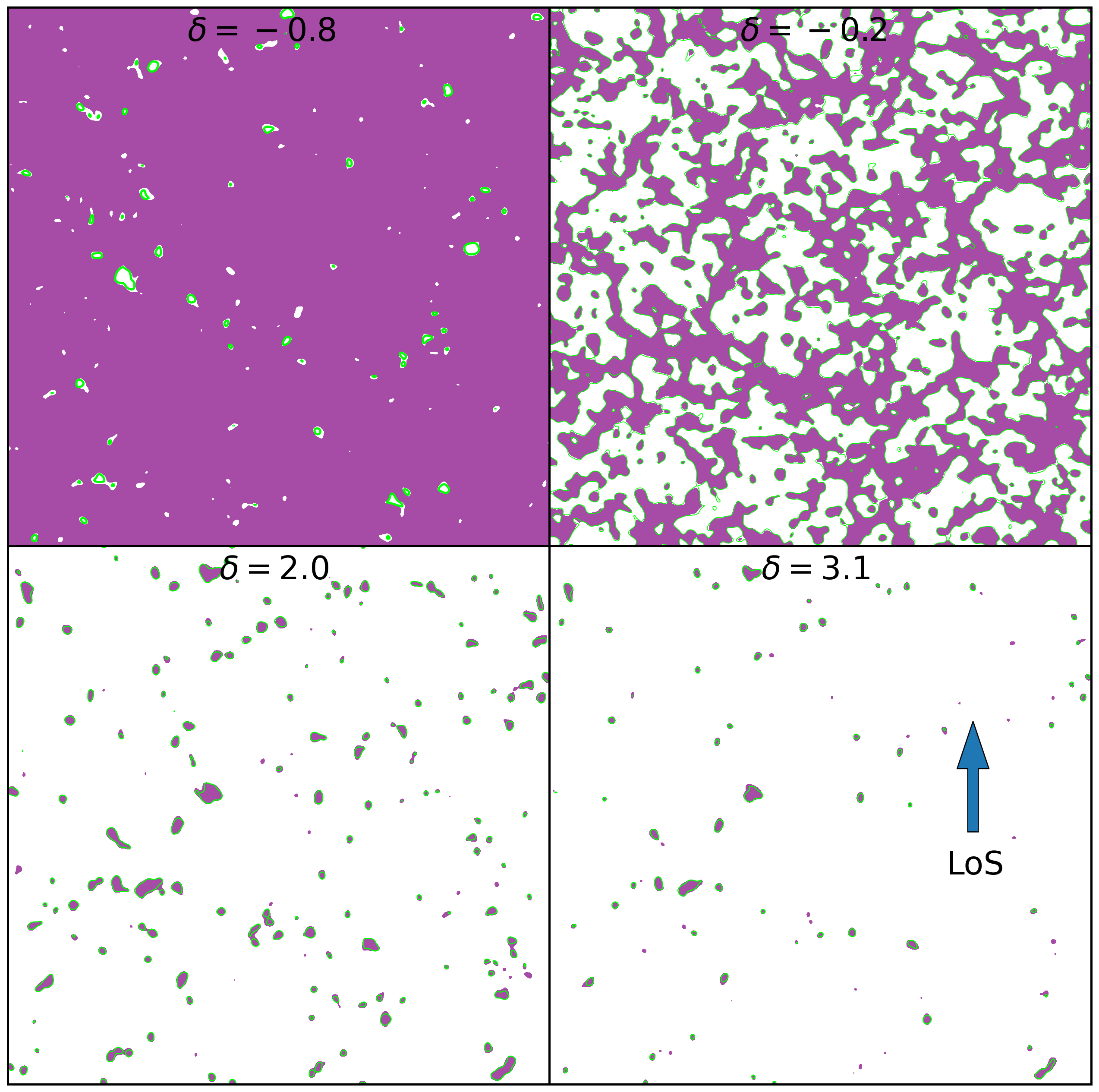
Figure 1: For 2D slices (thickness $2h^{-1}\rm Mpc$) of the redshift space 3D density field smoothed with $R_{G}=5h^{-1}\rm{Mpc}$, the 2D isodensity contours in a region of $1000\times 1000\ (h^{-1}\rm{Mpc})^{2}$ at the fiducial cosmology are plotted in green lines while the 2D excursion sets at the $f_{R}^{++++}$ cosmology are shown with purple regions. From the top left to bottom right, the four panels display plots for $\delta=-0.8,\ -0.2,\ 2.0,\$ and 3.1, respectively. The dominant structure in the four panels is thus voids, filaments, regions around clusters, and clusters.

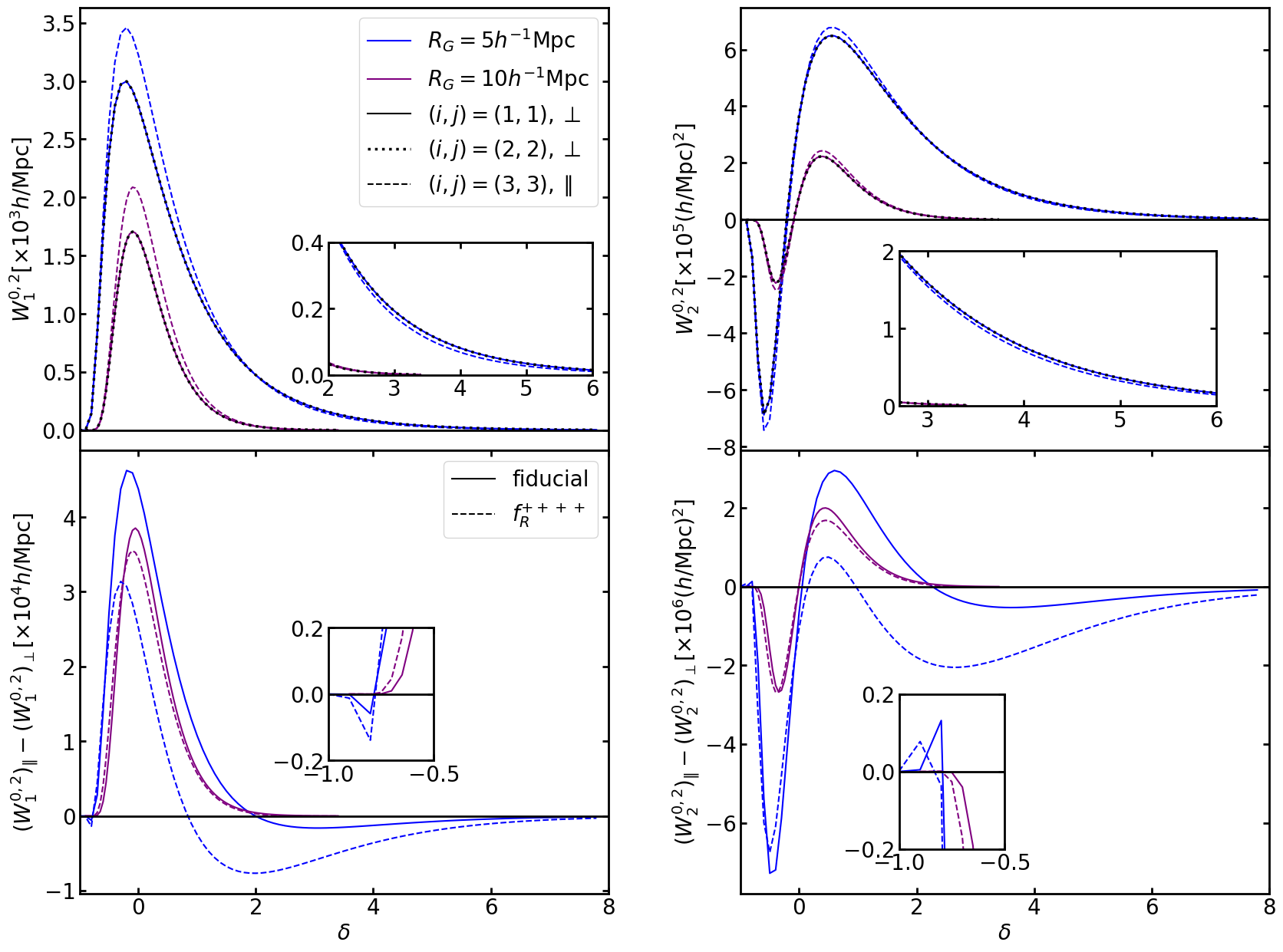
Figure 2: Top left panel: The perpendicular (solid and dotted lines, denoted as $(i,j)=(1,1),\ \perp$ and $(i,j)=(2,2),\ \perp$) and parallel component (dashed lines $(i,j)=(3,3),\ \parallel$) of $W_{1}^{0,2}$ are shown as functions of density threshold $\delta$. Blue for $R_{G}=5h^{-1}\rm{Mpc}$ and purple for $R_{G}=10h^{-1}\rm{Mpc}$. All curves in black are for $(i,j)=(2,2)$. The MTs are averaged over 5000 realizations at fiducial cosmology. Top right panel: Same as the top left panel, but for $W_{2}^{0,2}$. Bottom left panel: $(W_{1}^{0,2})_{\|}-(W_{1}^{0,2})_{\perp}$ for both fiducial (solid lines) and $f_{R}^{++++}$ (dashed lines) cosmology. The curves for $R_{G}=5,\ 10\ h^{-1}\rm{Mpc}$ are also plotted in blue and purple, respectively. Bottom right panel: Same as the bottom left panel, but for $W_{2}^{0,2}$.

To help understand the morphological and anisotropic information captured in the MTs, we plot in figure 1 both the 2D isodensity contour at the fiducial cosmology and the excursion set at the $f_{R}^{++++}$ cosmology for $\delta=-0.8$ (top left), $\delta=-0.2$ (top right), $\delta=2.0$ (bottom left), and $\delta=3.1$ (bottom right). These contours and regions are constructed from the redshift space density field smoothed with $R_{G}=5h^{-1}\rm{Mpc}$ and RSD applied along the vertical direction. The 3D MTs $W_{1}^{0,2}$ and $W_{2}^{0,2}$ are plotted in the left and right columes of figure 2, respectively. The three components of MTs are displayed in the first row, while the difference between the parallel and perpendicular elements is shown in the second row for both the fiducial and $f_{R}^{++++}$ cosmology. The overall shape of $W_{1}^{0,2}$ and $W_{2}^{0,2}$ follows that of $W_{1}$ and $W_{2}$, respectively, which measure the surface area and the mean curvature integral on the surface of the excursion set. Their amplitudes are larger when smaller smoothing scales are used because there are more details (thus more area elements) on the isodensity surfaces. For $W_{1}^{0,2}$, it can be understood why its value first increases with $\delta$, then peaks at $\delta\sim-0.2$, and finally decreases with $\delta$ by comparing the excursion sets shown in figure 2 at the four different thresholds. While for $W_{2}^{0,2}$, the mean curvature is negative for concave voids but positive for convex high-density regions and the transition from negative to positive happens in the intermediate density range.

Since we have applied the redshift space distortions along the z-axis, the line-of-sight component $(i,j)=(3,3)$ is different from the perpendicular $(i,j)=(1,1),\ (2,2)$ components, this can be seen for both $W^{0,2}_{1}$ and $W^{0,2}_{2}$. In addition, since $W_{1,2}=(W^{0,2}_{1,2})_{1,1}+(W^{0,2}_{1,2})_{2,2}+(W^{0,2}_{1,2})_{3,3}$, there exists overlapped information in the MFs $W_{1,2}$ and the MTs $W^{0,2}_{1,2}$. Thus we will only perform Fisher matrix analysis for either $W_{0}+W_{1}+W_{2}+W_{3}$ or $W_{0}+W_{1}^{0,2}+W_{2}^{0,2}+W_{3}$. On the other hand, $(W^{0,2}_{1,2})_{1,1}$ is statistically equal to $(W^{0,2}_{1,2})_{2,2}$ and they are statistically independent, their average $(W^{0,2}_{1,2})_{\perp}=((W^{0,2}_{1,2})_{1,1}+(W^{0,2}_{1,2})_{2,2})/2$ will have smaller uncertainty and will be used in the following Fisher matrix analysis, where the MTs will be composed of $(W_{1,2}^{0,2})_{\perp}=((W^{0,2}_{1,2})_{1,1}+(W^{0,2}_{1,2})_{2,2})/2$ and $(W_{1,2}^{0,2})_{\|}=(W_{1,2}^{0,2})_{3,3}$.

We can compare the RSD effects on LSS between the fiducial and $f_{R}^{++++}$ cosmology in both figure 1 and figure 2. For $\delta=-0.8$, voids (or more precisely, central regions of voids) are delineated by the contours and excursion sets. A slightly larger number of voids in both the fiducial and $f_{R}^{++++}$ cosmology appear elongated along the line of sight (LoS) in redshift space. This means the normal vector for the infinitesimal area elements of voids is more likely to be perpendicular to the LoS. That is, the integrant $n_{i}n_{j}$ in Eq 3.10 for $i=j=1$ or $i=j=2$ is larger than for $i=j=3$ most of the time when integrating over the surface of voids. On the other hand, the sign of $W_{2}^{0,2}$ is negative for voids. Therefore, $(W_{1}^{0,2})_{\|}-(W_{1}^{0,2})_{\perp}<0$ and $(W_{2}^{0,2})_{\|}-(W_{2}^{0,2})_{\perp}>0$, and can be seen in figure 2, although it is a very small signal. We can understand why voids are elongated in redshift space: since the surrounding CDM particles are moving out of these low-density regions; the particles farther from us are moving away from us, so they appear farther than they actually are; similarly, particles close to us are moving toward us, so they appear closer than they actually are [66, 67].

For $\delta=-0.2$, the cosmic structure is dominated by complicated filaments and it is thus hard to find out whether the filaments are squashed due to the Kaiser effect [64] or not. However, the bottom left panel of figure 2 tells us these structures are less flattened in the $f_{R}^{++++}$ than those in the fiducial cosmology. Many supporting examples can be easily found in the top right panel of figure 1, where the 2D isodensity contours at the fiducial cosmology appear more flattened along the LoS than the excursion sets at the $f_{R}^{++++}$ cosmology.

The Kaiser and FoG effects are competing against each other for intermediate density thresholds. For $\delta=2.0$, the FoG effect has already dominated on LSS for the $f_{R}^{++++}$ cosmology, while the two effects are equally strong in the fiducial cosmology. Therefore, we can see most of the high-density regions shown in the bottom left panel of figure 1 are elongated along the LoS in the $f_{R}^{++++}$ cosmology. However, these structures are either less stretched along the LoS or split into smaller and more isotropic islands in the fiducial cosmology. For $\delta=2.0$, the FoG effect finally wins and dominates in both the $f_{R}^{++++}$ and fiducial cosmology. And we can see the high-density regions are more elongated for $f_{R}^{++++}$ cosmology, this is because the fifth force makes the particles move faster, increasing the velocity dispersion and causing a stronger FoG effect compared to GR [68].

4 Fisher matrix formalism

We use the Fisher information matrix [69, 70] to quantify the constraining power of the statistics considered in this work on the cosmological parameters, which is defined as

$$F_{\alpha\beta}=\left\langle-\frac{\partial^{2}\ln\mathcal{L}}{\partial\theta_{\alpha}\partial\theta_{\beta}}\right\rangle,$$ (4.1)

where the likelihood $\mathcal{L}$ is assumed to be Gaussian. We will check in Appendix A the likelihood for all statistics and their combinations studied in this work can indeed be approximated by Gaussian. To avoid introducing artificial information, the covariance matrix of the observables $\boldsymbol{C}$ is assumed to be parameter-independent [71]. The Fisher matrix can then be written as

$$F^{stand}_{\alpha\beta}=\frac{\partial\boldsymbol{\mu}}{\partial\theta_{\alpha}}^{\mathrm{T}}\boldsymbol{C}^{-1}\frac{\partial\boldsymbol{\mu}}{\partial\theta_{\beta}},$$ (4.2)

where $\boldsymbol{\mu}$ is the theoretical mean for the data vector. It can be the power spectrum, MFs, MTs, and the combination of these statistics. $\boldsymbol{C}^{-1}$ is the inverse of the covariance matrix. To differentiate this estimator from the other two estimators that will be introduced in the following, we will call it the standard estimator of the Fisher matrix.

Recently, [72] finds the statistical noise in the numerical derivatives of observables can bias the Fisher forecast and underestimate the marginalized errors, the bias will be larger when higher-order forward differentiation schemes are used to estimate derivatives w.r.t. parameters like $M_{\nu}$. However, if we first compress the observables with the optimal compression scheme [73]

$$t_{\alpha}=\boldsymbol{\mu}_{\alpha}^{\mathrm{T}}\boldsymbol{C}^{-1}(\boldsymbol{d}-\boldsymbol{\mu}),\ \boldsymbol{\mu}_{\alpha}\equiv\frac{\partial\boldsymbol{\mu}}{\partial\theta_{\alpha}},$$ (4.3)

where $\boldsymbol{d}$ is the observable measured from a realization of simulations, and calculate the Fisher matrix for the compressed observable using the same equation as Eq 4.2, but replace the derivatives and covariance matrix with those for the compressed observable, then the Fisher matrix will be oppositely biased and overestimate the marginalized errors [74]. This new estimator is denoted with $F^{comp}$ and we will call it the compressed estimator hereafter, we will follow [74] and combine it with the standard estimator to give less biased (if not unbiased) forecasts

$$F^{comb}_{\alpha\beta}=G(F^{stand}_{\alpha\beta},F^{comp}_{\alpha\beta}),$$ (4.4)

where $G(A,B)$ is the geometric mean of matrix A and B, defined as

$$G(A,B)=A^{1/2}(A^{-1/2}BA^{-1/2})^{1/2}A^{1/2}.$$ (4.5)

Our Fisher matrix forecasts are all calculated with the combined estimator , we will present a comparison of the forecasts from the standard, compressed, combined estimator and use it as an additional convergence test in Appendix B.

4.1 Derivatives

For cosmological parameters, except the $f(R)$ parameter $f_{R_{0}}$ and the sum of neutrino masses $M_{\nu}$, the derivatives are estimated as

$$\frac{\partial\boldsymbol{\mu}}{\partial\theta_{\alpha}}\simeq\frac{\boldsymbol{\mu}(\theta_{\alpha}^{+})-\boldsymbol{\mu}(\theta_{\alpha}^{-})}{\theta_{\alpha}^{+}-\theta_{\alpha}^{-}},$$ (4.6)

where $\boldsymbol{\mu}(\theta_{\alpha}^{+})$ and $\boldsymbol{\mu}(\theta_{\alpha}^{-})$ are estimated as the average of observables from 500 realizations at $\theta_{\alpha}^{+}$ and $\theta_{\alpha}^{-}$, respectively. Since the values of $f_{R_{0}}$ are not distributed equally in both linear and log, we first perform the following change of variables: $f_{R_{0}}$ to $|f_{R_{0}}|^{\lg 2}$, so that the values of $f_{R_{0}}=0,\ -5\times 10^{-7},\ -5\times 10^{-6},\ -5\times 10^{-5},\ -5\times 10^{-4}$ map to $|f_{R_{0}}|^{\lg 2}=0,\ 0.0127,\ 0.0254,\ 0.0507,\ 0.101$. $f_{R_{0}}$ will still be used to refer to $|f_{R_{0}}|^{\lg 2}$ hereafter. Then the derivatives w.r.t. $f_{R_{0}}$ is estimated as

$$\frac{\partial\boldsymbol{\mu}}{\partial f_{R_{0}}}=\frac{\boldsymbol{\mu}(8df_{R_{0}})-12\boldsymbol{\mu}(4df_{R_{0}})+32\boldsymbol{\mu}(2df_{R_{0}})-21\boldsymbol{\mu}(\theta^{ZA}_{fid})}{12df_{R_{0}}},$$ (4.7)

where $df_{R_{0}}=0.0127$, and $\boldsymbol{\mu}(8df_{R_{0}})$, $\boldsymbol{\mu}(4df_{R_{0}})$, $\boldsymbol{\mu}(2df_{R_{0}})$, and $\boldsymbol{\mu}(\theta^{ZA}_{fid})$ are estimated with 500 realizations for model $f_{R}^{++++}$, $f_{R}^{+++}$, $f_{R}^{++}$, and Fiducial ZA, respectively. We don’t use simulations for $f_{R}^{+}$ because it is so close to fiducial cosmology that the difference in statistics between $f_{R}^{+}$ and GR will be dominated by noise [75]. For $M_{\nu}$, the derivative is constructed with

$$\frac{\partial\boldsymbol{\mu}}{\partial M_{\nu}}=\frac{\boldsymbol{\mu}\left(4dM_{\nu}\right)-\boldsymbol{\mu}\left(\theta_{fid}^{ZA}\right)}{4dM_{\nu}},$$ (4.8)

where $dM_{\nu}=0.1$eV, $\boldsymbol{\mu}(4dM_{\nu})$ and $\boldsymbol{\mu}(\theta_{fid}^{ZA})$ are estimated as the average of observables from 500 realizations at the $M_{\nu}=0.4eV$ cosmologies, and the fiducial cosmology with Zeldovich ICs, respectively. We choose this estimator because the noise in it is smaller than a similar estimator to Eq 4.7, which will give us a more convergent Fisher forecast [72]. We will discuss this in detail in Appendix B.

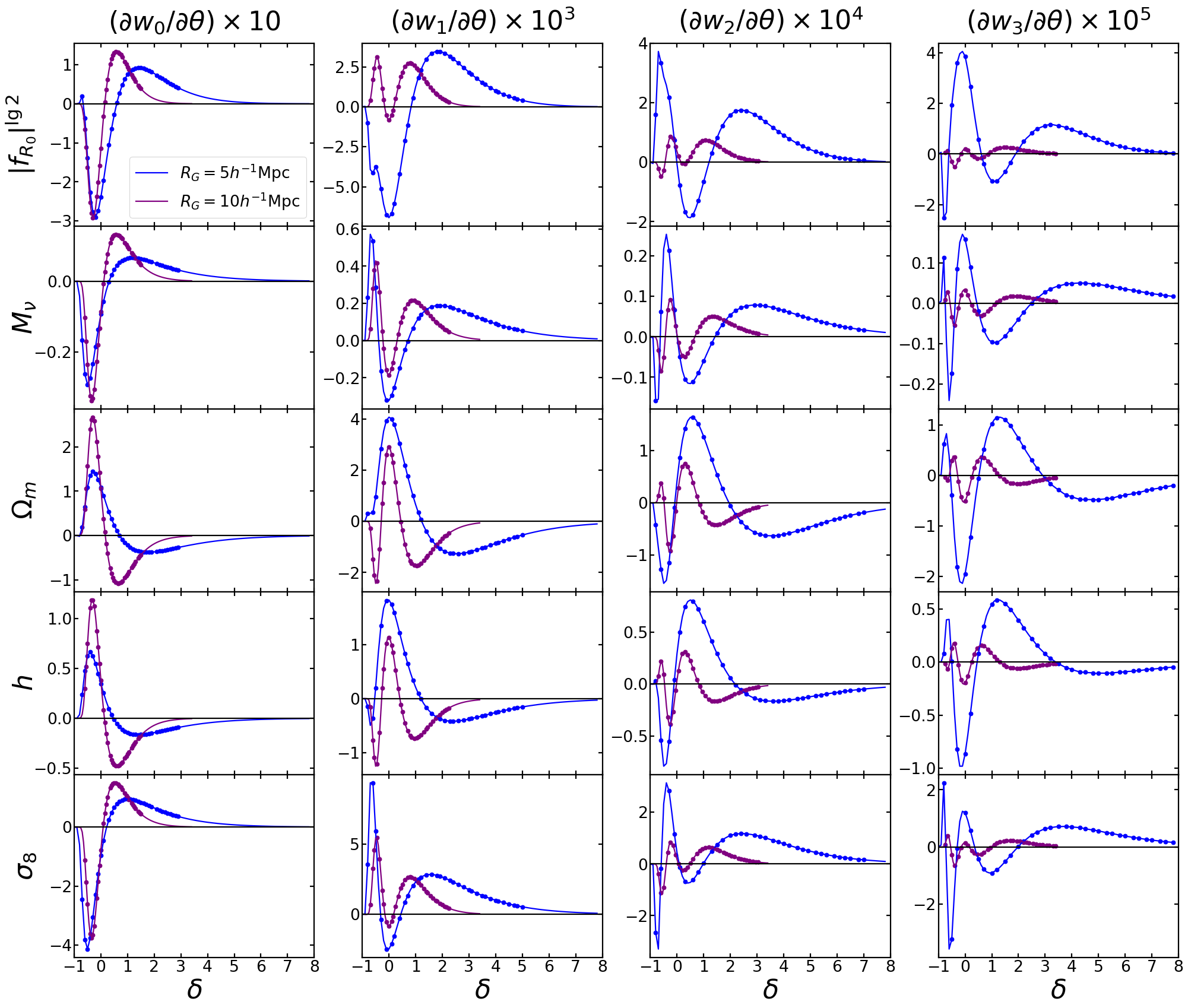
Figure 3: The numerical derivatives of the four 3D MFs w.r.t. the five cosmological parameters. The curves for $R_{G}=5,\ 10h^{-1}\rm{Mpc}$ are plotted in blue and purple. The dots plotted on the curves denote the data points that will be used in the Fisher forecast.

Figure 4: The numerical derivatives of the $(1,1)$ and $(3,3)$ components of the two 3D MTs $W_{1}^{0,2}$ (the first two columns) and $W_{2}^{0,2}$ (the last two columns) w.r.t. the five cosmological parameters. The curves for $R_{G}=5,\ 10h^{-1}\rm{Mpc}$ are plotted in blue and purple. The dots plotted on the curves denote the data points that will be used in the Fisher forecast. We note there also exists an evident difference between the $\perp$ and $\|$ components of both $\partial W^{0,2}_{1}/\partial\theta$ and $\partial W^{0,2}_{2}/\partial\theta$ for $|f_{R_{0}}|^{\lg 2}$.

For the data vector of the MFs and MTs, the thresholds are chosen based on the average statistics of 5000 fiducial simulations with the same binning scheme as that used in our previous work [49]: $N_{b}$ evenly spaced threshold bins are taken for $W_{0}$ in the range between $\delta_{0.01}$ to $\delta_{0.99}$, where the thresholds $\delta_{0.01}$ and $\delta_{0.99}$ correspond to the area (volume) fraction of 0.01 and 0.99, respectively. For other MFs and MTs, we first find the lower end of thresholds approximately corresponding to $1\%$ of the maximum of the statistics, $\delta_{low}$; and then find the higher end of thresholds where the curve is close to $1\%$ of the maximum of the statistics as well, $\delta_{high}$. Finally, $N_{b}$ evenly spaced threshold bins are taken in the range between $\delta_{low}$ to $\delta_{high}$. This threshold binning scheme tries to cover the variation range for each order of the statistics as extensively as possible while avoiding including the bins susceptible to noises and systematics.

For each of the monopole, quadrupole, and hexadecapole of the power spectrum, 80 wavenumber bins are used, up to $k_{\rm max}=0.5~{}h\rm{Mpc}^{-1}$. The size of each bin is $2\pi/L$, where $L=1h^{-1}\rm Gpc$ is the size of the simulation box.

In figure 3, we show the derivatives of the MFs w.r.t. the five cosmological parameters for two different smoothing scales $R_{G}=$ 5 (blue), 10 (purple) $h^{-1}\rm{Mpc}$. The data points chosen using the threshold binning scheme described above are marked with dots. It seems the curves in the low-density range are sparsely sampled with these points, but we find there is only a small change in the Fisher forecast when we increase the number of points in the low-density range. Since we explained in detail how the derivatives of the MFs change with the smoothing scale $R_{G}$ in [49], we will not repeat it here and only point out there are less distinct features in the derivatives for $R_{G}=10h^{-1}\rm{Mpc}$ than $R_{G}=5h^{-1}\rm{Mpc}$ because important structure information is smeared out when using the larger smoothing scale. Focus on the curves for $R_{G}=5h^{-1}\rm{Mpc}$, we find $\partial W_{i}/\partial\theta$ for $|f_{R_{0}}|^{\lg 2}$ is quite different from that for $M_{\nu}$ and the difference is most conspicuous for low-density thresholds: compared to $\partial W_{i}/\partial\theta$ for $M_{\nu}$, there is an extra peak on $\partial W_{0}/\partial\theta$ for $f_{R_{0}}$; a small wiggle rather than a peak lies on the left slope of the big valley of $\partial W_{1}/\partial\theta$; a small valley and a small peak are missing for $\partial W_{2}/\partial\theta$ and $\partial W_{3}/\partial\theta$, respectively. The overall shape of $\partial W_{i}/\partial\theta$ for $\Omega_{m}$ is close to that for $h$, but the difference in $\partial W_{1}/\partial\theta$ for low-density threshold can be easily detected by human eyes. The derivatives for $M_{\nu}$ and $\sigma_{8}$ are most similar, only varied height, depth, width, and position of peaks and valleys can be found by careful comparison. The strong degeneracy between $M_{\nu}$ and $\sigma_{8}$ will be broken when information from the total matter field is included [48, 76, 77, 78]. This degeneracy exists in both MFs and MTs for the CDM particle field, more convergent Fisher forecast results will be obtained if it is broken, as will be discussed in Appendix B.

Besides the morphological information captured in the MFs, we also plot the derivatives of the perpendicular and parallel components of $W^{0,2}_{1}$ and $W^{0,2}_{2}$ in figure 4, where we can directly see the anisotropic information contained in the MTs. The most important feature is a clear difference in $\partial(W^{0,2}_{1,2})_{\perp}/\partial\theta$ and $\partial(W^{0,2}_{1,2})_{\|}/\partial\theta$. The difference is largest for the derivative w.r.t. $|f_{R_{0}}|^{\lg 2}$, and second largest for $\Omega_{m}$, this is reasonable because the two parameters are most directly related to the growth rate of structure $f$, which is the MTs are sensitive to. The difference also means distinct information is embedded in the perpendicular and parallel elements of the MTs. We can expect that the parameter degeneracies will be broken by the combination of the $(W^{0,2}_{1,2})_{\perp}$ and $(W^{0,2}_{1,2})_{\|}$.

Similar to what has been found in the MFs, there are many characteristic signals in the derivatives of the MTs w.r.t. $|f_{R_{0}}|^{\lg 2}$, which are distinguished from those w.r.t. $M_{\nu}$. The curve for $\Omega_{m}$ shares a similar shape with that for $h$ in the high-density threshold range, but the difference in the derivatives for the very low-density range breaks the degeneracy between the two parameters. Unfortunately, this feature is smeared out when $R_{G}=10h^{-1}\rm{Mpc}$, which leads to a larger $\Omega_{m}-h$ degeneracy. We can find a consistent enhancement of the $\Omega_{m}-h$ degeneracy in the MTs from $R_{G}=5h^{-1}\rm{Mpc}$ to $R_{G}=10h^{-1}\rm{Mpc}$ in the contours plotted in Section 5.3. The strong degeneracy between $M_{\nu}$ and $\sigma_{8}$ still exists in the MTs, their derivatives only differ in the position, width, and amplitude of peaks and valleys on the curves.

4.2 Covariance matrix

We estimate the covariance matrices with 5000 fiducial simulations, which are found to be enough for converged parameter constraints in Appendix B. Due to uncertainties in the estimated covariance matrix $\hat{\mathbf{C}}$, the inverse of $\hat{\mathbf{C}}$ is not an unbiased estimator for $\mathbf{C}^{-1}$. Following [79], we remove the bias in $\hat{\mathbf{C}}^{-1}$ by

$$\mathbf{C}^{-1}=\frac{n-p-2}{n-1}\hat{\mathbf{C}}^{-1},$$ (4.9)

where p is the number of observables in the data vector, and n is the number of simulations used to estimate $\mathbf{C}$.

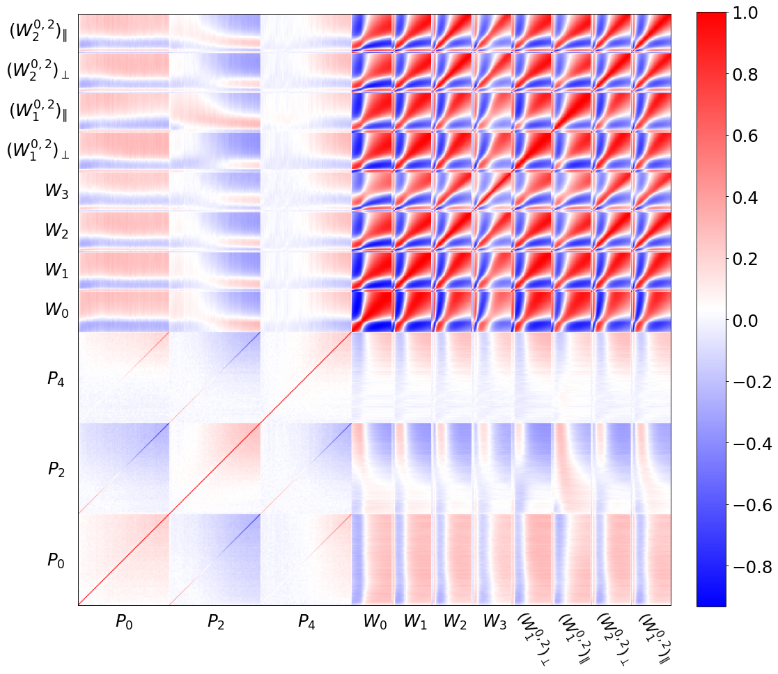
Figure 5: Correlation matrix of the monopole, quadrupole, and hexadecapole of the power spectrum ($P_{0},\ P_{2},\ P_{4}$), MFs ($W_{0},\ W_{1},\ W_{2},\ W_{3}$), and MTs ($W^{0,2}_{1},\ W^{0,2}_{2}$). For $P_{0},\ P_{2},\ P_{4}$, 80 wavenumber bins are used, up to $k_{\rm{max}}=0.5~{}h\mathrm{Mpc}^{-1}$. Only the MFs and MTs for $R_{G}=5h^{-1}\mathrm{Mpc}$ are included because they are very similar for $R_{G}=10h^{-1}\mathrm{Mpc}$. 35 threshold bins are taken for each order of MFs and each element of MTs. Bin values increase from left to right for each statistic. The correlation matrix is estimated using 5000 realizations of the fiducial model.

In figure 5, we show the correlation matrices of the data vector that combines the power spectrum ($P_{0}+P_{2}+P_{4}$), MFs ($W_{0},\ W_{1},\ W_{2},\ W_{3}$), and MTs ($W_{1}^{0,2},W_{2}^{0,2}$). For the power spectrum, 80 wavenumbers are used for each multipole, up to $k_{\rm max}=0.5h\ Mpc^{-1}$. For the MFs and MTs, 35 threshold bins are taken for each order of $W_{i}$, and each of $(W^{0,2}_{1})_{\perp}$, $(W^{0,2}_{1})_{\|}$, $(W^{0,2}_{2})_{\perp}$, $(W^{0,2}_{2})_{\|}$. Because there exists overlapped information in the MFs $W_{1,2}$ and the MTs $W^{0,2}_{1,2}$, we will only perform Fisher matrix analysis for either $W_{0}+W_{1}+W_{2}+W_{3}$ or $W_{0}+W_{1}^{0,2}+W_{2}^{0,2}+W_{3}$, a total of 140 or 210 bins will be used, respectively.

The correlation matrix of the power spectrum is shown in the left-bottom corner of figure 5. The auto-correlation of each multipole of the power spectrum has a simple structure: cross-correlation between different wavenumbers is weak on large scales (small $k$-bins, bottom left), but gradually strengthens on smaller scales. We can see a similar cross-correlation between the monopole and quadrupole to that between the quadrupole and the hexadecapole: the correlation is strong between multipoles in the same $k$-bin, and it is positive for small $k$-bins but negative for large $k$-bins; the correlation is weak and mainly negative between multipoles in varied $k$-bins. A weak cross-correlation can be seen between the monopole and the hexadecapole, it is close to zero for small $k$-bins and becomes positive for large $k$-bins. The small overall correlations between the power spectrum and the Minkowski statistics indicate that the Minkowski statistics can provide complementary information. The correlation matrix of the Minkowski statistics exhibits a much richer structure. The correlations between $W_{1,2}$ and $W_{1,2}^{0,2}$ as well as between perpendicular and parallel components of $W_{1,2}^{0,2}$ can be easily understood according to Eq 3.10 and Eq 3.11 ; while the correlation between $W_{1}^{0,2}$ and $W_{2}^{0,2}$ is quite similar to that between $W_{1}$ and $W_{2}$. Other correlations between the MFs with different threshold bins and orders are described in detail in our previous works [48, 49], thus are not given here.

When the Fisher matrix is calculated using the simulation-based method, a large number of simulations are needed for an accurate estimate of both the derivatives and covariance matrix to obtain converged parameter constraints [80, 81, 82]. In Appendix B, we will discuss this issue in more detail.

5 Results

We will first study how the anisotropic information is gathered in the Minkowski tensors in section 5.1, then investigate how the anisotropies captured by quadrupole and hexadecapole ($P_{2,4}$) of the power spectrum as well as by the MTs $W^{0,2}_{1,2}$ help break parameter degeneracies and tighten constraints in section 5.2, finally compare the power spectrum with the MFs plus MTs and discuss how their combination can improve constraints on modified gravity, massive neutrinos, and other parameters in section 5.3.

5.1 Information in the Minkowski tensors

Figure 6: Parameter constraints for $R_{G}=5h^{-1}\rm{Mpc}$ from the perpendicular ($(W_{1}^{0,2})_{\perp}+(W_{2}^{0,2})_{\perp}$, blue), parallel ($(W_{1}^{0,2})_{\|}+(W_{2}^{0,2})_{\|}$, red) component of MTs, and their combination ($W_{1}^{0,2}+W_{2}^{0,2}$, green). The contours for high- and low-density thresholds are plotted with solid and dashed lines.

In section 3.2, we have discussed the effect of RSD on isodensity contours for different thresholds. Three kinds of characteristic imprints of RSD on LSS are seen for $R_{G}=5h^{-1}\rm{Mpc}$: a slightly larger number of voids are elongated along LoS for very low-density thresholds; the more complicated contours are squashed along LoS due to the Kaiser effect for intermediate thresholds; and the FoG effect is seen for large thresholds where the high-density regions are also elongated along LoS. In contrast, the LSS is dominated by the Kaiser effect in the whole threshold range for $R_{G}=10h^{-1}\rm{Mpc}$. Therefore, we will only present results for $R_{G}=5h^{-1}\rm{Mpc}$ in this section, because we want to compare the information content of the MTs dominated by the Kaiser effect with that dominated by the FoG effect . The Kaiser effect captured by the MTs on linear scales is studied in [52, 53], where they found it is sensitive to the linear growth rate of the LSS, as shown in Eq 3.12 and Eq 3.13. The information content in the MTs from the small-scale FoG effect is investigated and compared with that from the Kaiser effect in this work for the first time. We note that the information from the small-scale FoG effect is discussed in [83] with the 2-point correlation function. The RSD effect in different density environments is also studied in [84].

For a fair comparison, 15 evenly spaced threshold bins are taken in the range between $\delta_{low}$ and $\delta=2$ for “low-density thresholds”, while 15 threshold bins are also evenly taken from $\delta>2$ to $\delta_{high}$ for “high-density thresholds”. $\delta_{low}$ and $\delta_{high}$ is the same as the threshold binning scheme described in Section 4.1, while $\delta=2$ is where the sign of $(W_{1}^{0,2})_{\|}-(W_{1}^{0,2})_{\perp}$ changes at the fiducial cosmology, it is also where the dominated RSD effect transits from the Kaiser effect to the FoG effect.

Due to the anisotropies introduced by RSD, distinct information is captured by $(W_{i}^{0,2})_{\perp}$ and $(W_{i}^{0,2})_{\|}$, this can be seen for both high- and low-density thresholds in figure 6. The perpendicular and parallel elements of MTs show varied sensitivity to the same parameter and different parameter degeneracy for the same parameter pair. Tighter constraints can thus be obtained by the combination of $(W_{i}^{0,2})_{\perp}$ and $(W_{i}^{0,2})_{\|}$. We note the perpendicular MTs always give tighter constraints on all parameters than the parallel ones for the low-density thresholds, this is mainly due to smaller uncertainty in $(W^{0,2}_{1,2})_{\perp}$. As has been explained in Section 3.2, it is the average of the first two statistically independent elements of the MTs: $(W^{0,2}_{1,2})_{\perp}=((W^{0,2}_{1,2})_{1,1}+(W^{0,2}_{1,2})_{2,2})/2$. However, smaller statistical noise doesn’t always mean smaller marginalized errors on cosmological parameters. Even with larger variance, $(W^{0,2}_{1,2})_{\|}$ beats $(W^{0,2}_{1,2})_{\perp}$ at the constraint on $\sigma_{8}$ for high-density thresholds where the FoG effect dominates.

On the other hand, more distinct and complementary information is embedded in the MTs of low and high-density thresholds. For each of $(W_{i}^{0,2})_{\perp}$, $(W_{i}^{0,2})_{\|}$, and their combination, nearly all constraints obtained from statistics of the low thresholds are stronger than those from high-density thresholds. The constraint of $(W_{i}^{0,2})_{\perp}$ on $|f_{R_{0}}|^{\lg 2}$ is the only exception, for which the constraints from the low and high thresholds are comparable to each other. It is expected that statistics of low-density regions are sensitive to $f_{R_{0}}$ due to the smaller screening effect in low-density regions [85, 22, 86]. The comparable constraining power on the f(R) parameter of $(W_{i}^{0,2})_{\perp}$ for low and high thresholds may indicate rich information about $f_{R_{0}}$ can also be found from intermediate- and high-density regions. The constraint on $M_{\nu}$ is consistent with [78], where they found void size function has stronger constraining power on $M_{\nu}$ than the halo mass function. This can be understood because the effect of massive neutrinos on the LSS is strongest in low-density regions [87, 88].

To summarize, complementary information is found in the perpendicular and parallel elements of the MTs as well as in the MTs for low- and high-density thresholds. The combination of them will provide the MFs with anisotropic information, and help tighten constraints on the f(R) parameter and other parameters.

5.2 Information in real- and redshift-space

Figure 7: Parameter constraint contours from the isotropic statistics and the combination of isotropic and anisotropic statistics on large scales ($k_{\rm{max}}=0.25~{}h\rm{Mpc}^{-1},\ R_{G}=10~{}h^{-1}\rm{Mpc}$, the first row) and small scales ($k_{\rm{max}}=0.5~{}h\rm{Mpc}^{-1},\ R_{G}=5~{}h^{-1}\rm{Mpc}$, the second row). Results for $P_{0}$ and $W_{0}+W_{1}+W_{2}+W_{3}$ of real space field are shown with grey and blue filled ellipses, while results for statistics in redshift space are plotted with lines: dotted, dashed, and solid black lines for $P_{0}$, $P_{0,2}$, and $P_{0,2,4}$, dotted and dashed cyan lines for $W_{0}+W_{1}+W_{2}+W_{3}$ and $W_{0}+W^{0,2}_{1}+W^{0,2}_{2}+W_{3}$.

For cosmological models with different values of neutrino masses and modified gravity parameters, those with a comparable matter power spectrum at a given time can have different growth rates [27, 29]. Motivated by this finding, we will compare the sensitivity of statistics in real space with that in redshift space and investigate how the constraining power on the f(R) parameter, neutrino mass, and other parameters is strengthened when anisotropic information is included. We note that the Fisher forecast present in figure 7 and discussed in this section is performed for the four parameters $\{|f_{R_{0}}|^{\lg 2},M_{\nu},\Omega_{m},\sigma_{8}\}$, the value of $h$ is fixed because the strong degeneracy between $h$ and $\Omega_{m}$ in the real-space MFs makes us fail to get a very converged Fisher forecast for the full five parameters. The relation between parameter degeneracies in the statistic and the convergence of its Fisher forecast will be discussed in Appendix B.

As can be seen in figure 7, strong degeneracies exist in the real space power spectrum monopole ($P_{0}$ r-space) between $|f_{R_{0}}|^{\lg 2}$ and $\{M_{\nu},\Omega_{m},\sigma_{8}\}$ for both large (weakly non-linear) and small (non-linear) scales. These degeneracies are only slightly weakened on large scales but significantly reduced on small scales in the redshift-space power spectrum monopole ($P_{0}$). Therefore, we observe comparable constraints from $P_{0}$ in real- and redshift-space on large scales but much tighter constraints from $P_{0}$ in redshift space than real space, on small scales.

There is a different story for the MFs. Similar parameter degeneracies and constraints are obtained from the MFs in real- and redshift-space for both large and small scales. However, this is only true when the Fisher forecast is performed for $\{|f_{R_{0}}|^{\lg 2},M_{\nu},\Omega_{m},\sigma_{8}\}$. Extra information is indeed captured by the MFs in redshift-space so that the degeneracy between $\Omega_{m}$ and $h$ is broken, that is why we can obtain converged Fisher matrix forecasts for the full five parameters when we focus on statistics in redshift space.

When anisotropic information contained in $P_{2}$ and $P_{4}$ is added, we can see the parameter degeneracies are gradually reduced, and parameter constraints are improved. The anisotropic information in $P_{2}$ is important for all parameters on large scales but only important for the f(R) parameter and $\Omega_{m}$ on small scales. Anisotropies captured by $P_{4}$ are only helpful for $|f_{R_{0}}|^{\lg 2}$ and $\Omega_{m}$ on both large and small scales.

The anisotropic information captured by the MTs can only slightly help improve sensitivity to $|f_{R_{0}}|^{\lg 2}$ and $\Omega_{m}$ on both large and small scales. There are three possible explanations for this: first, the MFs already contain considerable non-Gaussian information related to the growth rate so that only a small part of information leaks into anisotropic information; second, the MTs used in this work only capture a small part of anisotropies, we need other independent rank-2 MTs or even higher rank MTs to extract more anisotropies [89]; third, a large part of anisotropies in the redshift space are smeared out by the Gaussian window function, this can be directly seen in figure 1, where the RSD effect is barely perceptible by human eyes.

5.3 Comparison and combination of the power spectrum and MTs

Figure 8: Parameter constraint contours from the power spectrum $P_{0,2,4}$ (black), the MTs $W_{0}+W^{0,2}_{1}+W^{0,2}_{2}+W_{3}$ (blue), and the combination of the power spectrum and MTs $P_{0,2,4}+W_{0}+W^{0,2}_{1}+W^{0,2}_{2}+W_{3}$ (green). Results for small scales ($k_{\rm max}=0.5~{}h\rm{Mpc}^{-1},\ R_{G}=5~{}h^{-1}\rm{Mpc}$) and large scales ($k_{\rm max}=0.25~{}h\rm{Mpc}^{-1},\ R_{G}=10~{}h^{-1}\rm{Mpc}$) are plotted in solid and dashed lines, respectively.

Statistic	$P_{0,2,4}$	$W_{0}+W^{0,2}_{1,2}+W_{3}$	$P_{0,2,4}+W_{0}+W^{0,2}_{1,2}+W_{3}$	$P_{0,2,4}$	$W_{0}+W^{0,2}_{1,2}+W_{3}$	$P_{0,2,4}+W_{0}+W^{0,2}_{1,2}+W_{3}$
Scale	$k_{\rm max}=0.5~{}h\rm{Mpc}^{-1},\ R_{G}=5~{}h^{-1}\rm{Mpc}$			$k_{\rm max}=0.25~{}h\rm{Mpc}^{-1},\ R_{G}=10h^{-1}\rm{Mpc}$
$\Omega_{m}$	0.014	0.005	0.004	0.022	0.016	0.008
$h$	0.032	0.016	0.011	0.049	0.053	0.022
$\sigma_{8}$	0.032	0.011	0.010	0.043	0.016	0.013
$M_{\nu}$	0.572	0.185	0.171	0.766	0.276	0.223
$|f_{R_{0}}|^{\lg 2}$	0.0009	0.0008	0.0005	0.0040	0.0036	0.0026

Table 2: Marginalized parameter constraints for statistics on small scales (the first three columns, $k_{\rm max}=0.5~{}h\rm{Mpc}^{-1},\ R_{G}=5~{}h^{-1}\rm{Mpc}$) and large scales (the last three columns, $k_{\rm max}=0.25~{}h\rm{Mpc}^{-1},\ R_{G}=10~{}h^{-1}\rm{Mpc}$), from the power spectrum $P_{0,2,4}$ (first and forth columns), the MTs $W_{0}+W^{0,2}_{1,2}+W_{3}$ (second and fifth columns), and the combination of power spectrum and MTs $P_{0,2,4}+W_{0}+W^{0,2}_{1,2}+W_{3}$ (third and last columns).

Statistic	$P_{0,2,4}/(W_{0}+W^{0,2}_{1,2}+W_{3})$	$P_{0,2,4}/(P_{0,2,4}+W_{0}+W^{0,2}_{1,2}+W_{3})$	$P_{0,2,4}/(W_{0}+W^{0,2}_{1,2}+W_{3})$	$P_{0,2,4}/(P_{0,2,4}+W_{0}+W^{0,2}_{1,2}+W_{3})$
Scale	$k_{\rm max}=0.5~{}h\rm{Mpc}^{-1},\ R_{G}=5~{}h^{-1}\rm{Mpc}$		$k_{\rm max}=0.25~{}h\rm{Mpc}^{-1},\ R_{G}=10~{}h^{-1}\rm{Mpc}$
$\Omega_{m}$	2.6	3.4	1.4	2.8
$h$	2.0	3.0	0.9	2.2
$\sigma_{8}$	3.0	3.3	2.7	3.4
$M_{\nu}$	3.1	3.3	2.8	3.4
$|f_{R_{0}}|^{\lg 2}$	1.0	1.9	1.1	1.5

Table 3: Marginalized parameter constraint improvements for the power spectrum on small scales (the first two columns, $k_{\rm max}=0.5~{}h\rm{Mpc}^{-1},\ R_{G}=5~{}h^{-1}\rm{Mpc}$) and large scales (the last two columns, $k_{\rm max}=0.25~{}h\rm{Mpc}^{-1},\ R_{G}=10~{}h^{-1}\rm{Mpc}$), from the MTs $W_{0}+W^{0,2}_{1,2}+W_{3}$ (first and third columns), and the combination of power spectrum and MTs $P_{0,2,4}+W_{0}+W^{0,2}_{1,2}+W_{3}$ (second and last columns).

We have shown the improvement from MTs is not effective for MFs. In this section, we will focus on how the non-Gaussian information from the MTs (“MTs” will refer to $W_{0}+W_{1}^{0,2}+W_{2}^{0,2}+W_{3}$ hereafter in this section) helps break the degeneracies between $|f_{R_{0}}|^{\lg 2}$ and $M_{\nu}$ and between other parameter pairs on both large and small scales. The marginalized $68\%$ Fisher matrix confidence contours from the power spectrum multipoles ($P_{0,2,4}$), MTs ($W_{0}+W_{1}^{0,2}+W_{2}^{0,2}+W_{3}$), combination of power spectrum and MTs ($P_{0,2,4}+W_{0}+W_{1}^{0,2}+W_{2}^{0,2}+W_{3}$) on large ($k_{\rm max}=0.25~{}h\rm{Mpc}^{-1},\ R_{G}=10~{}h^{-1}\rm{Mpc}$) and small ($k_{\rm max}=0.5~{}h\rm{Mpc}^{-1},\ R_{G}=5~{}h^{-1}\rm{Mpc}$) scales are shown in figure 8. The corresponding parameter constraints from these statistics on the two scales are also listed in table 2. For a better comparison, the ratio of constraints from the power spectrum to those from the MTs as well as to those from the combination $P_{0,2,4}+W_{0}+W_{1}^{0,2}+W_{2}^{0,2}+W_{3}$ is present in table 3, also for both the small and large scales.

Before comparing the constraining power of the power spectrum and MTs, we shall clarify that there is no exact correspondence between the smoothing scale used for the MTs and the $k_{\rm max}$ choice for the power spectrum. In practice, the smallest smoothing scale $R_{G}=5~{}h^{-1}\rm{Mpc}$ is the scale where we believe the algorithm used to measure the MTs is accurate enough (see Section 3.2 for a more detailed explanation). We also note that whether the modes $k>0.5~{}h\rm{Mpc}^{-1}$ are included or not only make a $0\%$, $1\%$, $2\%$, and $3\%$ difference in the amplitude of the $W_{0}$, $W_{1}$, $W_{2}$, and $W_{3}$ for $R_{G}=5~{}h^{-1}\rm{Mpc}$. This indicates the information in the MTs may be indeed dominated by modes $k\leq 0.5~{}h\rm{Mpc}^{-1}$. A fairer comparison between constraints from the power spectrum and the MTs could be made if we also implemented a sharp k-filter on top of the Gaussian smoothing following [75]. The sharp k-filter can lead to a slight increase in the errors. Therefore, we may slightly overestimate the improvements in parameter constraints of the power spectrum from the MTs or their combination.

On large scales, the constraints from $P_{0,2,4}$ on $\Omega_{m}$, $h$, and $|f_{R_{0}}|^{\lg 2}$ are comparable with those from the MTs, and the MTs have stronger constraining power on $M_{\nu}$ and $\sigma_{8}$. The overall smaller degeneracies among all parameters (it is hard to see whether the degeneracy between $M_{\nu}$ and $\sigma_{8}$ become weaker or not for the MTs in figure 8, but we find the correlation coefficient between $M_{\nu}$ and $\sigma_{8}$ is -0.997 for $P_{0,2,4}$ and -0.958 for the MTs) in the MTs significantly help tighten parameter constraints from $P_{0,2,4}$ by a factor of 2.8, 2.2, 3.4, 3.4, and 1.5 for $\Omega_{m}$, $h$, $\sigma_{8}$, $M_{\nu}$, $|f_{R_{0}}|^{\lg 2}$, when combining $P_{0,2,4}$ and the MTs.

On small scales, the velocity information captured by $P_{0,2,4}$ breaks the degeneracy between the f(R) parameter and other parameters. A comparable constraint on $|f_{R_{0}}|^{\lg 2}$ with that from the MTs can thus be achieved with the power spectrum alone. However, strong degeneracies still exist in the power spectrum among $\Omega_{m}$, $h$, $\sigma_{8}$, and $M_{\nu}$. The degeneracies in the MTs among all parameters are smaller than those in $P_{0,2,4}$, which is the same as what is found on large scales. Non-Gaussian information captured by the MTs is more sensitive to the four parameters apart from $|f_{R_{0}}|^{\lg 2}$, and 2.6, 2.0, 3.0, and 3.1 times tighter constraints are obtained from the MTs alone than those from the power spectrum. The high sensitivity of the MTs to the four parameters, together with the different degeneracies among parameters in the MTs from those in $P_{0,2,4}$, are why a factor of 3.4, 3.0, 3.3, 3.3, and 1.9 of improvement in the power spectrum constraints on $\Omega_{m}$, $h$, $\sigma_{8}$, $M_{\nu}$, and $|f_{R_{0}}|^{\lg 2}$ is achieved by the combination of $P_{0,2,4}$ and the MTs.

Focusing on the f(R) parameter and neutrino mass, first on large scales, the MTs help break the $|f_{R_{0}}|^{\lg 2}-M_{\nu}$ degeneracy existing in the $P_{0,2,4}$ but its constraint on $|f_{R_{0}}|^{\lg 2}$ is moderately improved by a factor of 1.5 by the combination of the power spectrum and MTs. This improvement is smaller than that on small scales, where the constraint of $P_{0,2,4}$ on $|f_{R_{0}}|^{\lg 2}$ is improved by a factor of 1.9 because more non-Gaussian information is contained in the MTs on small scales than on large scales. We have shown that the distinct imprints left on the LSS by f(R) gravity in [39] and by massive neutrinos in [48] can be captured by the MFs on small scales. By the measurement of MFs at multiple density thresholds, the effect of f(R) gravity and massive neutrinos on voids, filaments, and high-density regions is detected by the MFs, and thus by the MTs.

6 Discussions

Also based on the Quijote and Quijote-MG simulations, [75] conducted Fisher forecasts using the WST coefficients and the power spectrum in real space at $z=0$. The Fisher analysis is performed for $\{\Omega_{m},\ \Omega_{b},\ h,\ n_{s},\ \sigma_{8},\ M_{\nu},\ |f_{R_{0}}|^{\lg 2}\}$, therefore the comparison between results present in this work and that work may not be fair because the degeneracies between $\Omega_{m},\ h,\ \sigma_{8},\ M_{\nu},\ |f_{R_{0}}|^{\lg 2}$ and $\Omega_{b},\ n_{s}$ are not included in this work. We find tighter constraints on $|f_{R_{0}}|^{\lg 2}$ from the power spectrum multipoles and MTs in redshift space compared with that from the power spectrum monopole and WST coefficients. This is expected because the velocity information captured by the power spectrum multipoles and MTs helps increase their sensitivity to the f(R) parameter. In addition, the degeneracies between $f_{R_{0}}$ and $\Omega_{b},\ n_{s}$ may also weaken the constraints on the f(R) parameter obtained from the WST coefficients.

The idea of using kinematic information to break the degeneracy between $M_{\nu}$ and $f_{R_{0}}$ was first proposed in [27], they found the kinematic information related to both the growth rate on large scales and the virial velocities inside of collapsed structures are well suited to constrain deviations from general relativity without being affected by the effect of massive neutrinos. This is consistent with our findings in Section 5.1, we find both the anisotropic information captured by the MTs of low-density regions, where the Kaiser effect dominates, and that captured by the MTs of high-density regions, where the FoG effect dominates, are sensitive to the f(R) parameter in the presence of massive neutrinos. Following this idea, [29, 28] investigated the possibility of breaking the degeneracy between massive neutrinos and f(R) gravity model using RSD with the monopole and quadrupole of 2-point statistics in redshift space. We have discussed this topic in Section 5.2 and found the degeneracy between $M_{\nu}$ and $f_{R_{0}}$ can be reduced even with the monopole of power spectrum alone in redshift space, the degeneracy can be broken further when the quadrupole is included, and there still exists extra information about $f_{R_{0}}$ in the hexadecapole. In addition, the anisotropies captured by the MTs can improve the constraining power of the MFs on the f(R) parameter.

Alternative statistics apart from the power spectrum and two-point correlation functions of particles, halos, or galaxies are also explored for 3D LSS [85, 22, 25, 23, 24, 90]. However, a direct comparison between their results and ours is difficult because none of them has derived a constraint on $M_{\nu}$ and $f_{R_{0}}$ at the same time. Section 5.3 has quantified the improvement from non-Gaussian information captured by the MTs for both non-linear and quasi-linear scales. We find the non-Gaussian information is important to constrain $M_{\nu}$ and $f_{R_{0}}$ at the same time on these scales.

7 Conclusions

We are at the beginning of the Stage-IV era of precision cosmology, the current and upcoming cosmological observations of the cosmic large-scale structure of the Universe may enable the detection of massive neutrinos and modifications of the gravity model at the same time. In this work, we investigate the possibility of tightly constraining the mass sum of neutrinos and the f(R) gravity model simultaneously with the structure and velocity information extracted using the power spectrum multipoles and Minkowski tensors.

As the first application of the tensor Minkowski functionals in cosmology on fully non-linear scales, we first describe and interpret in detail how the effect of redshift-space distortions on low, intermediate, and high-density regions is captured by the 3D MTs; then the influence of $f_{R_{0}}$, $M_{\nu}$, and other cosmological parameters on the MTs are compared and the non-degenerate imprints of $f_{R_{0}}$ and $M_{\nu}$ are found on the MTs; finally, to analyze the information embedded in the MTs, we quantify the information content in the perpendicular and parallel element of the MTs for both low and high-density regions with the Fisher information formalism, which helps us understand how the anisotropic information dominated by the Kaiser and FoG effect can put constraints on $f_{R_{0}}$ and $M_{\nu}$ and other cosmological parameters.

Motivated by previous works, we also study how the velocity information helps break the degeneracy between $f_{R_{0}}$ and $M_{\nu}$. The velocity information is added into the CDM field by the redshift-space distortion, which is then measured by all of the statistics used in this work. The power spectrum monopole, although as an isotropic statistic, can still detect the effect of RSD and thus extract a part of velocity information. Therefore, we see the $f_{R_{0}}$ and $M_{\nu}$ degeneracy is already reduced in the redshift space power spectrum monopole. However, the constraining power of the MFs mainly comes from the captured non-Gaussianities, no significant difference in the sensitivity to $f_{R_{0}}$ and $M_{\nu}$ is seen between real- and redshift-space. With the quadrupole and hexadecapole of the power spectrum and the MTs, more velocity information is extracted and stronger constraints are obtained, especially for the f(R) parameter.

To extend our previous works, we do a comparison between constraints from the power spectrum and the MTs instead of the MFs alone and investigate how the combination of the power spectrum and the MTs helps improve the constraints from $P_{0,2,4}$. We find that the non-Gaussian information indeed is helpful to break the $f_{R_{0}}$ and $M_{\nu}$ degeneracy, which is consistent with other works based on other non-Gaussian statistics. The MTs, similar to what has been found for the MFs [62, 48, 49], can provide complementary information for the power spectrum and tighten the constraints significantly for all of the parameters considered in this work on both quasi- and non-linear scales.

Tighter constraints can be obtained if we extend our analysis to smaller scales, as indicated by Figure 7 of [75]. However, we choose only to include k-modes up to $k_{\rm{max}}=0.5~{}h\rm{Mpc}^{-1}$, considering the finite resolution of simulations used in this work. For the MTs, the smoothing scale should be at least larger than the average distance between particles [91, 92, 93, 46], which is about $2h^{-1}\rm{Mpc}$ for the simulations used here. On the other hand, the smoothing scale $R_{G}=5h^{-1}\rm{Mpc}$ is the smallest scale we can use to get rid of the discretization error of iso-density contour generation algorithm used in this work [51]. A finer density field is required if we want to extend the analysis to scales smaller than $R_{G}=5h^{-1}\rm{Mpc}$ and extend the analysis to higher-rank Minkowski tensors capable of extracting more anisotropic information. However, the computation time will exceed what we can afford for such an analysis. Better results can also be calculated by combining the MTs with different smoothing scales, we don’t discuss it in this work because it is already studied in our previous work [48, 49]. A more interesting extension of this work will be to combine statistics at different redshift because it has been found in previous works [22, 28] that the degeneracy between massive neutrinos and the f(R) gravity may be more easily disentangled at higher redshifts.

The reliability of the Fisher forecast depends on both the Gaussianity of the likelihood of the statistics and the convergence of results w.r.t. the noise in the derivatives and covariance matrix as well as the inherent error in the numerical differentiation methods. We have discussed these topics in Appendices A, B, C and showed our analysis presented in this work has passed all of these tests. A more conservative result which has the best convergence is presented and discussed in Appendices D.

In reality, the observed galaxy positions are distorted by their peculiar velocities along LoS and the LoS vector varies at different points in space. This differs from the plane-parallel approximation used in this work when applying the RSD in the simulations, where a common LoS vector is shared at each point in the field. However, the effect of RSD on the MTs beyond the plane-parallel approximation is discussed only on linear and quasi-linear scales in [53]. Besides the RSD effect, the Alcock-Paczynski (AP) distortions, the complicated geometry, and other systematics of galaxy surveys can introduce extra anisotropies into the field. In addition, the model of the halo-galaxy connection and the emulation of their dependence on both cosmological and halo-galaxy connection parameters should also be taken into consideration in order to apply the MTs to galaxy catalogs from spectroscopic surveys. We leave the investigation for these topics to future work.

Appendix A Gaussianity test

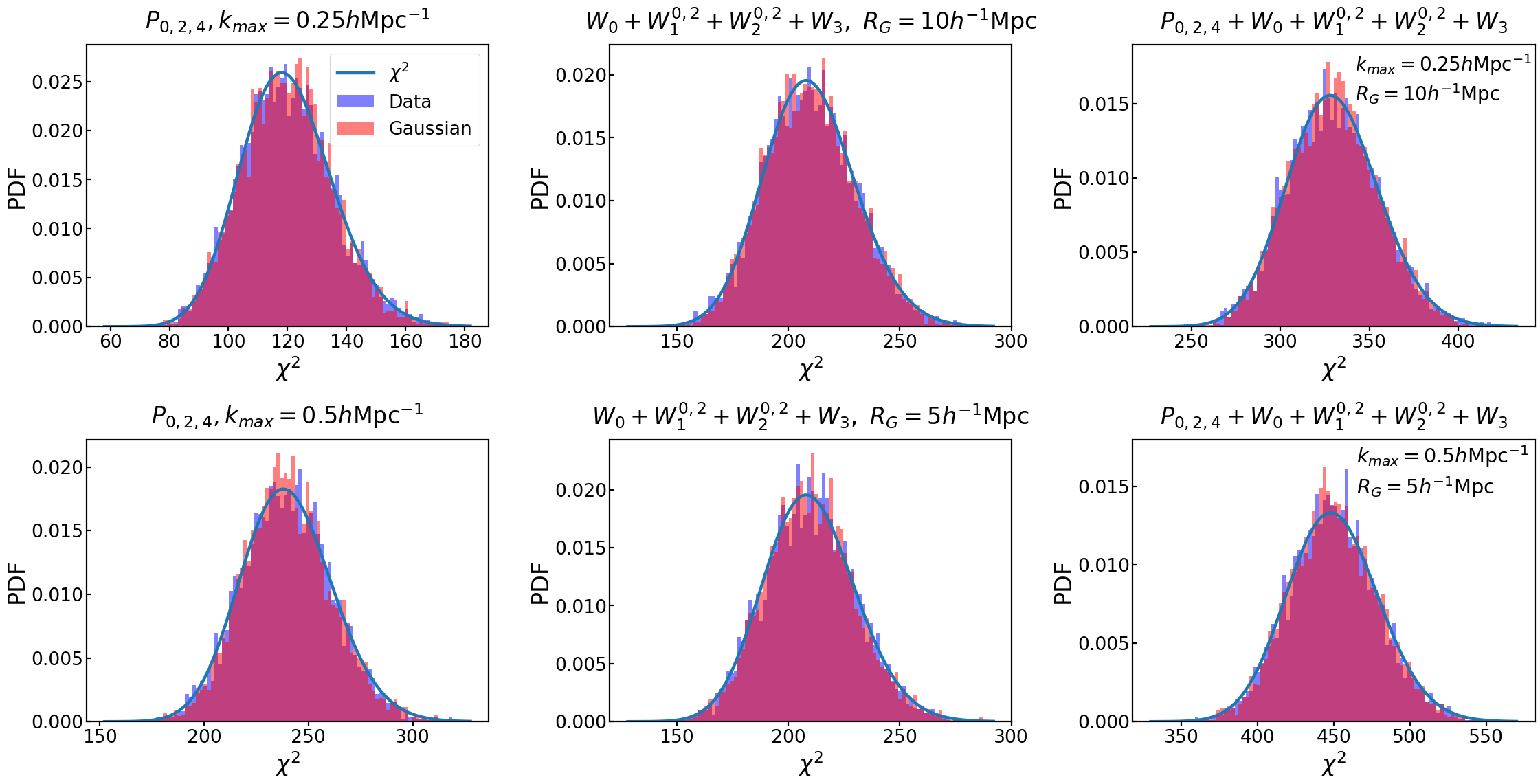
Figure 9: A qualitative assessment of the Gaussianity of the likelihood for the power spectrum multipoles ($P_{0,2,4}$, first column), the MTs ($W_{0}+W_{1}^{0,2}+W_{2}^{0,2}+W_{3}$, second column), and their combination ($P_{0,2,4}+W_{0}+W_{1}^{0,2}+W_{2}^{0,2}+W_{3}$, third column) for large ($k_{\rm{max}}=0.25~{}h\rm{Mpc}^{-1}$, $R_{G}=10~{}h^{-1}\rm{Mpc}$, first row) and small ($k_{\rm{max}}=0.5~{}h\rm{Mpc}^{-1}$, $R_{G}=5~{}h^{-1}\rm{Mpc}$, second row) scales. The histograms of the $\chi^{2}$ values measured from the Quijote simulations are drawn in blue, while those of the $\chi^{2}$ values measured from a multivariate Gaussian distribution with the same mean and covariance as the Quijote simulations are shown in red. The solid lines show theoretical $\chi^{2}$ distributions with degrees of freedom equal to the length of observables.

It was reported in [94] that non-Gaussianities in the likelihood of statistics might lead to artificially tight bounds on the cosmological parameters using the Fisher matrix formalism. To access the Gaussianity of the likelihood of the statistics used in this work, we follow the analysis performed in [95, 96] and check that the likelihood of these statistics can be approximated by the multivariate Gaussian. Since we have 5000 fiducial simulations, we can obtain 5000 $\chi^{2}$ values for each of the statistics by

$$\chi^{2}_{i}=(\boldsymbol{d_{i}}-\boldsymbol{\mu})^{T}C^{-1}(\boldsymbol{d_{i}}-\boldsymbol{\mu}),$$ (A.1)

where $\boldsymbol{d_{i}}$ is the data vector of the summary statistics for the $i$-th simulation, $\boldsymbol{\mu}$ and $C$ is the mean and the covariance matrix of the data vector estimated from the 5000 simulations.

If the assumption of Gaussian likelihood holds, the $\chi^{2}$ values are expected to follow a $\chi^{2}$ distribution with degrees of freedom equal to the length of the data vector. In figure 9, we plot the histogram (in blue) of the $\chi^{2}$ values measured from the Quijote simulations and compare it with the theoretical $\chi^{2}$ distribution curve for each of the summary statistics and their combination. Due to the existence of fluctuations in the histogram, the curve may not exactly agree with the histogram, even for a sample strictly following the $\chi^{2}$ distribution. To visualize the amplitude of the fluctuations around the theoretical $\chi^{2}$ distribution curve and use it as a ruler to help assess the Gaussianity of the data vectors, we create 5000 multivariate Gaussian distributed data vectors with the same mean and covariance matrix as those estimated from the fiducial simulations. We then obtain 5000 $\chi^{2}$ values for the multivariate Gaussian distributed data vectors and also plot a histogram (in red) for them in figure 9. As seen in this figure, the histogram of $\chi^{2}$ values for all statistics is very close to that for the Gaussian distributed data vectors and agrees well with the theoretical $\chi^{2}$ distribution curve. This indicates that the likelihood of the power spectrum, MTs, and their combination on both small and large scales can be well modeled as Gaussian.

Appendix B Convergence w.r.t. noise in derivatives and covariance matrix

Figure 10: The “Fisher correlation matrix” calculated using $P_{0,2,4}$ with $k_{\rm{max}}=0.25~{}h\rm{Mpc}^{-1}$ (top left panel) and $k_{\rm{max}}=0.5~{}h\rm{Mpc}^{-1}$ (bottom left panel) as well as using $W_{0}+W_{1}^{0,2}+W_{2}^{0,2}+W_{3}$ with $R_{G}=10h^{-1}\rm{Mpc}$ (top right panel) and $R_{G}=5h^{-1}\rm{Mpc}$ (bottom right panel) for $\Omega_{m}$, $\Omega_{b}$, $h$, $n_{s}$, $\sigma_{8}$, $M_{\nu}$ and $f_{R_{0}}$.

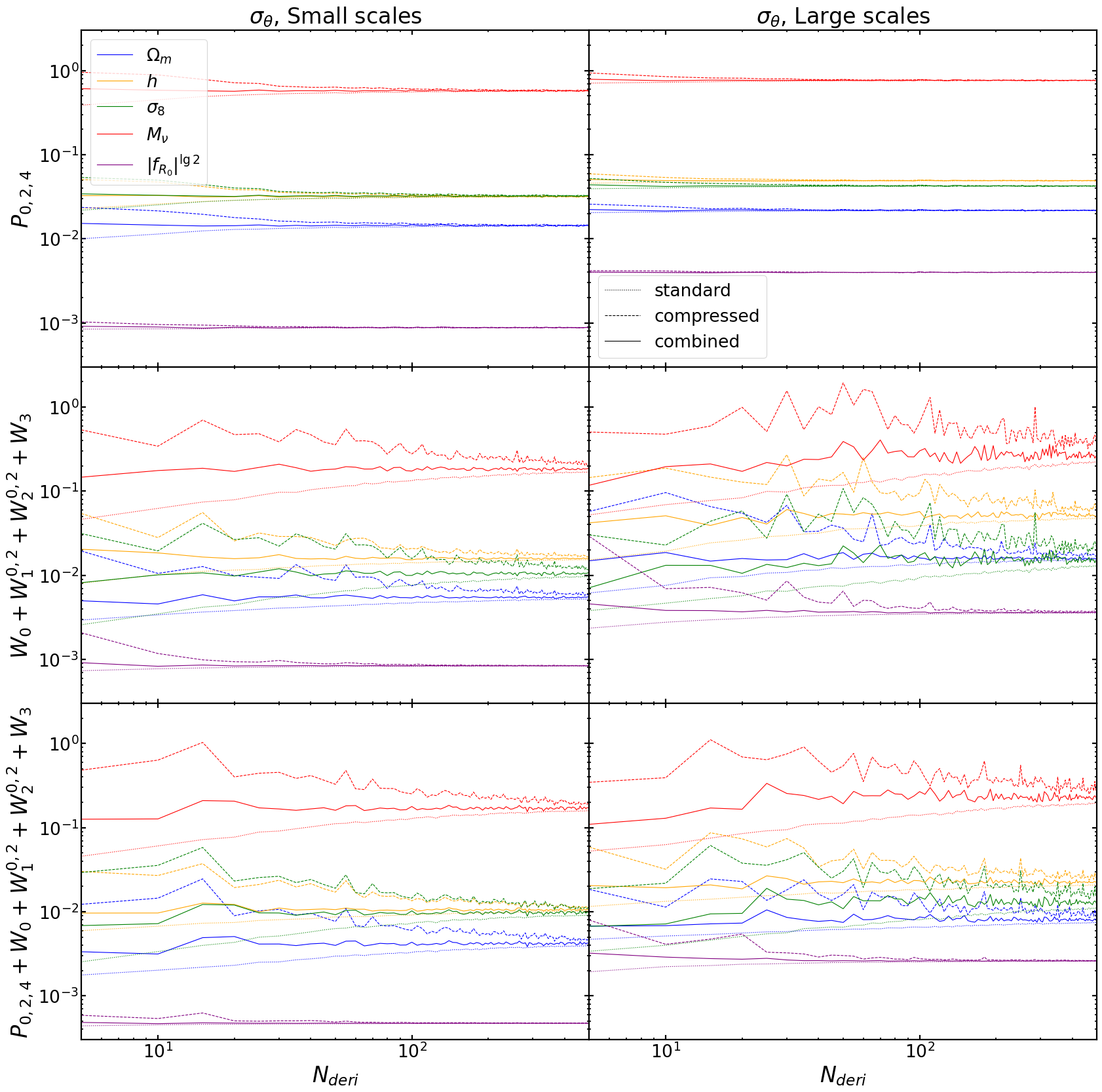
Figure 11: Convergence of the marginalized errors from the power spectrum multipoles ($P_{0,2,4}$, first row), the MTs ($W_{0}+W^{0,2}_{1}+W^{0,2}_{1}+W_{3}$, second row), and their combination ($P_{0,2,4}+W_{0}+W^{0,2}_{1}+W^{0,2}_{1}+W_{3}$, third row) on $\Omega_{m}$, $h$, $\sigma_{8}$, $M_{\nu}$ and $f_{R_{0}}$ (blue, orange, green, red, purple) for both small ($k_{\rm{max}}=0.5~{}h\rm{Mpc}^{-1},\ R_{G}=5~{}h^{-1}\rm{Mpc}$, left column) and large ($k_{\rm{max}}=0.25~{}h\rm{Mpc}^{-1},\ R_{G}=10~{}h^{-1}\rm{Mpc}$, right column) scales. The Fisher forecasts are obtained with derivatives estimated from $N_{deri}$ simulations using the standard, compressed, and combined estimator (dotted, dashed, and solid lines). These forecasts are all based on covariance matrices estimated with $N_{cov}=5000$ simulations.

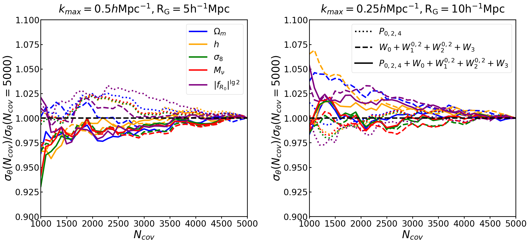
Figure 12: Convergence of the marginalized errors from the power spectrum multipoles ($P_{0,2,4}$, dotted lines), the MTs ($W_{0}+W^{0,2}_{1}+W^{0,2}_{2}+W_{3}$, dashed lines), and their combination ($P_{0,2,4}+W_{0}+W^{0,2}_{1}+W^{0,2}_{2}+W_{3}$, solid lines) on $\Omega_{m}$, $h$, $\sigma_{8}$, $M_{\nu}$ and $f_{R_{0}}$ (in blue, orange, green, red, purple), for both small ($k_{\rm{max}}=0.5~{}h\rm{Mpc}^{-1},\ R_{G}=5~{}h^{-1}\rm{Mpc}$, left column) and large ($k_{\rm{max}}=0.25~{}h\rm{Mpc}^{-1},\ R_{G}=10~{}h^{-1}\rm{Mpc}$, right column) scales. $\sigma_{\theta}(N_{cov})/\sigma_{\theta}(N_{cov}=5000)$ is the ratio of Fisher forecasts obtained with covariance matrices estimated from $N_{cov}$ simulations to those obtained with covariance matrices estimated from $N_{cov}=5000$ simulations. These forecasts are based on derivatives estimated with $N_{deri}=500$ simulations. The horizontal dashed lines correspond to $\sigma_{\theta}(N_{cov})/\sigma_{\theta}(N_{cov}=5000)=1$.

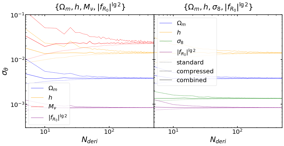
Figure 13: Convergence of the marginalized errors from the MTs ($W_{0}+W^{0,2}_{1}+W^{0,2}_{1}+W_{3}$) when the Fisher analysis is performed for $\{\Omega_{m},\ h,\ M_{\nu},\ f_{R_{0}}^{\lg 2}\}$ (left column) and $\{\Omega_{m},\ h,\ \sigma_{8},\ f_{R_{0}}^{\lg 2}\}$ (right column). The Fisher forecasts are obtained with derivatives estimated from $N_{deri}$ simulations using the standard, compressed, and combined estimator (dotted, dashed, and solid lines). These forecasts are all based on covariance matrices estimated with $N_{cov}=5000$ simulations.

The Fisher matrix forecast, as a computationally efficient and reliable tool, has been widely used in cosmology to estimate the precision with which model parameters can be measured [97, 98, 99, 100]. It can be simply calculated for a set of observables, if both the covariance matrix of these observables and derivatives of each observable w.r.t. parameters are known. However, the noise and bias in both the covariance matrix and derivatives can be propagated into the Fisher matrix, leading to unreliable and biased forecasts [101, 102, 74, 72]. Here in this appendix, we will explain in which situation the Fisher forecasts are most prone to noise, and convergence tests will be done to show why our forecast is converged and reliable.

With the Fisher matrix, the marginalized parameter constraints are given by

$$\sigma_{\alpha}=\sqrt{(F^{-1})_{\alpha\alpha}}.$$ (B.1)

Let us write the Fisher matrix as the following block matrix structure

$$\left[F_{\alpha\beta}\right]=\left[\begin{array}[]{ll}F_{\mu\nu}&F_{\mu b}\\ F_{a\nu}&F_{ab}\end{array}\right],$$ (B.2)

the determinant of the Fisher matrix is then given by

$$\det(F_{\alpha\beta})=\det(F_{\mu\nu})\det(F_{ab}-F_{a\nu}F^{-1}_{\nu\mu}F_{\mu b}).$$ (B.3)

When the matrix block $F_{\mu\nu}$ is calculated for two strongly degenerate parameters like $\sigma_{8}$ and $M_{\nu}$, $\det(F_{\mu\nu})$ will be very close to zero, and the determinant of the full Fisher matrix $\det(F_{\alpha\beta})$ will also approach zero. Since the parameter covariance matrix is obtained by inverting the Fisher matrix; thus, small uncertainties in the Fisher matrix may result in much larger deviations in the parameter covariance matrix. The degeneracies can be detected in advance with the “Fisher correlation matrix”

$$f_{\alpha\beta}=F_{\alpha\beta}/\sqrt{F_{\alpha\alpha}F_{\beta\beta}}.$$ (B.4)

If the non-diagonal element of $f_{\alpha\beta}$ is close to -1 or 1, it indicates the degeneracy between the two corresponding parameters may lead to an amplification of error for the inverse of the Fisher matrix. In Figure 10, we show the Fisher correlation matrix for both the power spectrum and MTs on both large and small scales. Strong degeneracies can be seen in all of the four panels among $\Omega_{b}$, $h$, and $n_{s}$, as well as between $\sigma_{8}$ and $M_{\nu}$. To get a convergent and reliable Fisher forecast, we have to fix two of the three parameters $\Omega_{b}$, $h$, and $n_{s}$ and use Eq 4.8 for the estimate of derivatives w.r.t. $M_{\nu}$ instead of the higher order numerical differentiation schemes to reduce the influence of the derivative noise [72].

The uncertainties of the Fisher matrix stem from the noises existing in both the estimated derivatives and covariance matrix. We will check how the marginalized errors vary when increasing the number of simulations used to estimate the derivatives $N_{\rm deri}$ in figure 11 and the covariance matrix $N_{\rm cov}$ in figure 12. For the convergence w.r.t. $N_{deri}$, we compare the forecasts calculated with the standard, compressed, and combined estimator described in Section 4 for the five parameters $\Omega_{m}$, $h$, $\sigma_{8}$, $M_{\nu}$, and $|f_{R_{0}}|^{\lg 2}$ on both small and large scales. For $P_{0,2,4}$, the results from the three estimators agree with each other very well on both small and large scales when $N_{deri}>100$. On the other hand, for the same estimator, the forecasts calculated with different $N_{deri}$ agree with each other as well. Therefore, figure 11 provides a dual convergence check for the Fisher matrix analysis. For $W_{0}+W_{1}^{0,2}+W_{2}^{0,2}+W_{3}$, differences can be seen even for $N_{deri}=500$ in the constraints on the four parameters except $|f_{R_{0}}|^{\lg 2}$ from the three estimators, but the constraints from the standard and compressed estimator provide an approximate lower and upper bound for the forecasts [74]. In addition, the constraints from the combined estimator for different $N_{deri}$ agree with each other when $N_{deri}>100$, even though there exist some fluctuations for $h$, $\sigma_{8}$ and $M_{\nu}$ in the constraints on large scales. For the combination of the power spectrum and MTs, the convergence is dominated by that of the MTs, we thus see very similar convergence curves to those of the MTs.

A great convergence with respect to $N_{cov}$ can be seen in figure 12, the ratio $\sigma_{\theta}(N_{cov})/\sigma_{\theta}(N_{cov}=5000)$ is smaller than $7.5\%$ ($2.5\%$) for both statistics and their combination on both small and large scales for all parameters when $N_{cov}>1000$ ($N_{cov}>3000$).

As shown in figure 10, both the degeneracy among $\Omega_{b}$, $h$ and $n_{s}$ and between $\sigma_{8}$ and $M_{\nu}$ are a potential source of instability when inverting the Fisher matrix to get parameter constraints. And we have shown in figure 11 if we rest the degeneracy among $\Omega_{b}$, $h$ and $n_{s}$ by fixing $\Omega_{b}$ and $n_{s}$ and only including $h$ in the Fisher analysis, we can already get converged forecasts for all cases considered in this work. In figure 13, we further rest the degeneracy between $\sigma_{8}$ and $M_{\nu}$ and only perform the Fisher analysis for either $\{\Omega_{m},\ h,\ M_{\nu},\ |f_{R_{0}}|^{\lg 2}\}$ or $\{\Omega_{m},\ h,\ \sigma_{8},\ |f_{R_{0}}|^{\lg 2}\}$ with the MTs. We find the results from the three estimators agree with each other well when $N_{deri}>300$ for the two Fisher analyses performed. For the left panel, the derivative w.r.t. $M_{\nu}$ is estimated with the highest order of differentiation scheme, and converged results can still be obtained even though the highest order estimator of the $M_{\nu}$ derivative is most prone to noise.

Appendix C Convergence w.r.t. inherent error of numerical differentiation methods

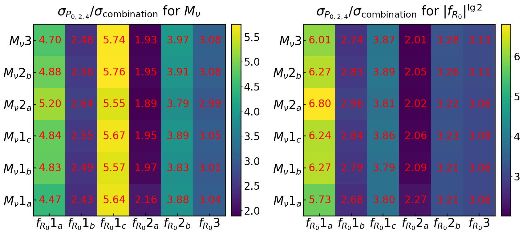
Figure 14: Improvement in parameter constraints of $P_{0,2,4}$ from the combination of $P_{0,2,4}$ and MTs for $M_{\nu}$ (left panel) and $|f_{R_{0}}|^{\lg 2}$ (right panel). The constraint improvements are plotted as a function of the estimator type of the $f_{R_{0}}$ (x-axis) and $M_{\nu}$ (y-axis) derivatives.

Two different kinds of errors exist in the estimate of derivatives with cosmological simulations: the first one comes from the cosmic variance, which is the fluctuations of observables among different realizations of the simulations; the second one is the inherent error of the numerical differentiation methods, it depends on the step size and the order of the differentiation method. We have discussed the first kind of error in the AppendixB and will investigate the second kind here.

Because the $f_{R}^{+}$ model is so close to fiducial cosmology that the difference in statistics between $f_{R}^{+}$ and GR will be dominated by noise, we won’t use it for the estimate of derivatives w.r.t. $f_{R_{0}}$. With the simulations list in Table 1, we can estimate the derivatives w.r.t. $f_{R_{0}}$ with:

$$f_{R_{0}}1_{a}:\frac{\partial\boldsymbol{\mu}}{\partial f_{R_{0}}}=\frac{\boldsymbol{\mu}(8df_{R_{0}})-\boldsymbol{\mu}(\theta^{ZA}_{fid})}{8df_{R_{0}}},$$ (C.1)

$$f_{R_{0}}1_{b}:\frac{\partial\boldsymbol{\mu}}{\partial f_{R_{0}}}=\frac{\boldsymbol{\mu}(4df_{R_{0}})-\boldsymbol{\mu}(\theta^{ZA}_{fid})}{4df_{R_{0}}},$$ (C.2)

$$f_{R_{0}}1_{c}:\frac{\partial\boldsymbol{\mu}}{\partial f_{R_{0}}}=\frac{\boldsymbol{\mu}(2df_{R_{0}})-\boldsymbol{\mu}(\theta^{ZA}_{fid})}{2df_{R_{0}}},$$ (C.3)

$$f_{R_{0}}2_{a}:\frac{\partial\boldsymbol{\mu}}{\partial f_{R_{0}}}=\frac{-\boldsymbol{\mu}(8df_{R_{0}})+4\boldsymbol{\mu}(4df_{R_{0}})-3\boldsymbol{\mu}(\theta^{ZA}_{fid})}{8df_{R_{0}}},$$ (C.4)

$$f_{R_{0}}2_{b}:\frac{\partial\boldsymbol{\mu}}{\partial f_{R_{0}}}=\frac{-\boldsymbol{\mu}(4df_{R_{0}})+4\boldsymbol{\mu}(2df_{R_{0}})-3\boldsymbol{\mu}(\theta^{ZA}_{fid})}{4df_{R_{0}}},$$ (C.5)

$$f_{R_{0}}3:\frac{\partial\boldsymbol{\mu}}{\partial f_{R_{0}}}=\frac{\boldsymbol{\mu}(8df_{R_{0}})-12\boldsymbol{\mu}(4df_{R_{0}})+32\boldsymbol{\mu}(2df_{R_{0}})-21\boldsymbol{\mu}(\theta^{ZA}_{fid})}{12df_{R_{0}}},$$ (C.6)

where $df_{R_{0}}=0.0127$, and $\boldsymbol{\mu}(8df_{R_{0}})$, $\boldsymbol{\mu}(4df_{R_{0}})$, $\boldsymbol{\mu}(2df_{R_{0}})$, and $\boldsymbol{\mu}(\theta^{ZA}_{fid})$ are estimated with 500 realizations for model $f_{R}^{++++}$, $f_{R}^{+++}$, $f_{R}^{++}$, and Fiducial ZA, respectively. The derivatives w.r.t. $M_{\nu}$ can be similarly estimated with the equations listed above, but to differentiate them from those for $f_{R_{0}}$, we label them with $M_{\nu}1_{a}$, $M_{\nu}1_{b}$, $M_{\nu}1_{c}$, $M_{\nu}2_{a}$, $M_{\nu}2_{b}$, and $M_{\nu}3$, respectively.

In figure 14, we compare the improvements in constraints of $P_{0,2,4}$ from the combination of $P_{0,2,4}$ and MTs on both $M_{\nu}$ and $f_{R_{0}}$ when the $M_{\nu}$ and $f_{R_{0}}$ derivatives are calculated with different estimators. For both $M_{\nu}$ and $f_{R_{0}}$, the variation of methods for the $M_{\nu}$ derivatives only mildly change the results, but the improvements differ significantly when changing the schemes for the $f_{R_{0}}$ derivatives. However, if we only focus on the results when the calculation of the $f_{R_{0}}$ derivatives excludes simulations at the $f_{R}^{++}$ cosmology, that is, compare the results for $f_{R_{0}}1_{a}$, $f_{R_{0}}1_{b}$, and $f_{R_{0}}2_{a}$, we can find the results converged to those for $f_{R_{0}}2_{a}$. On the other hand, a convergence trend can also be found focusing on results for $f_{R_{0}}1_{c}$, $f_{R_{0}}2_{b}$, and $f_{R_{0}}3$, where simulations at the $f_{R}^{++}$ cosmology are included. We choose to trust the Fisher forecasts calculated with the derivative estimator $f_{R_{0}}3$ because it has the smallest step size and the highest order, which means it is supposed to have the smallest inherent error existing in the numerical differentiation methods.

Appendix D A more conservative result

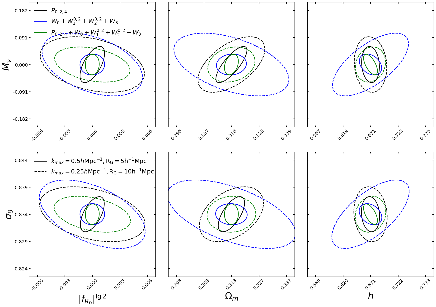
Figure 15: Parameter constraint contours for $\{\Omega_{m},\ h,\ M_{\nu},\ |f_{R_{0}}|^{\lg 2}\}$ (first row) and $\{\Omega_{m},\ h,\ \sigma_{8},\ |f_{R_{0}}|^{\lg 2}\}$ (second row). Results for the power spectrum $P_{0,2,4}$, the MTs $W_{0}+W^{0,2}_{1}+W^{0,2}_{2}+W_{3}$, and the combination of power spectrum and MTs $P_{0,2,4}+W_{0}+W^{0,2}_{1}+W^{0,2}_{2}+W_{3}$ are plotted with black, blue, and green lines, respectively. Solid and dashed lines for small scales ($k_{\rm{max}}=0.5~{}h\rm{Mpc}^{-1},R_{G}=5~{}h^{-1}\rm{Mpc}$) and large scales ($k_{\rm{max}}=0.25~{}h\rm{Mpc}^{-1},R_{G}=10~{}h^{-1}\rm{Mpc}$).

The strong degeneracy between $\sigma_{8}$ and $M_{\nu}$ can make the Fisher matrix ill-conditioned and the noise in the derivatives and covariance matrix may be significantly amplified. Although we have done the convergence tests in Appendix B to show converged results can be obtained even when the $\sigma_{8}$ and $M_{\nu}$ degeneracy is included in the Fisher matrix analysis, we will still present a more conservative Fisher forecast in this appendix.

In figure 15, we provide the parameter confidence contours when the Fisher matrix analysis is done for either $\{\Omega_{m},\ h,\ M_{\nu},\ |f_{R_{0}}|^{\lg 2}\}$ or $\{\Omega_{m},\ h,\ \sigma_{8},\ |f_{R_{0}}|^{\lg 2}\}$. In the first case, constraints from the MTs are weaker on $\Omega_{m}$, $h$, and $M_{\nu}$, but stronger on $|f_{R_{0}}|^{\lg 2}$ than those from $P_{0,2,4}$ on large scales. The constraining power of the MTs is only slightly weaker on $h$ than $P_{0,2,4}$ on small scales. In the second case, smaller errors can be seen from $P_{0,2,4}$ on all the four parameters on large scales; but the MTs are more sensitive to $\sigma_{8}$ and $|f_{R_{0}}|^{\lg 2}$ on small scales. No matter in which case, on which scale, complementary information can be found from the MTs to $P_{0,2,4}$. Degeneracies are broken and tighter constraints are obtained with the combination of the power spectrum and MTs.

Comparing figure 15 with figure 8, we find the constraining power of $P_{0,2,4}$ is mainly limited by the $\sigma_{8}$ and $M_{\nu}$ degeneracy, and much tighter constraints could be obtained if the degeneracy is broken. The small-scale MTs are very sensitive to $M_{\nu}$ and $\sigma_{8}$, and tight constraints can be obtained no matter the degeneracy between $M_{\nu}$ and $\sigma_{8}$ is on or off. They are also sensitive to $|f_{R_{0}}|^{\lg 2}$, so tighter or comparable constraints can be derived in general from the MTs compared with those from $P_{0,2,4}$.

References

- [1] D. N. Spergel, L. Verde, H. V. Peiris, E. Komatsu, M. R. Nolta, C. L. Bennett et al., First-Year Wilkinson Microwave Anisotropy Probe (WMAP) Observations: Determination of Cosmological Parameters, ApJS 148 (2003) 175 [astro-ph/0302209].
- [2] G. Hinshaw, D. Larson, E. Komatsu, D. N. Spergel, C. L. Bennett, J. Dunkley et al., Nine-year Wilkinson Microwave Anisotropy Probe (WMAP) Observations: Cosmological Parameter Results, ApJS 208 (2013) 19 [1212.5226].
- [3] Planck Collaboration, N. Aghanim, Y. Akrami, M. Ashdown, J. Aumont, C. Baccigalupi et al., Planck 2018 results. VI. Cosmological parameters, A&A 641 (2020) A6 [1807.06209].
- [4] S. Alam, M. Aubert, S. Avila, C. Balland, J. E. Bautista, M. A. Bershady et al., Completed SDSS-IV extended Baryon Oscillation Spectroscopic Survey: Cosmological implications from two decades of spectroscopic surveys at the Apache Point Observatory, Phys. Rev. D 103 (2021) 083533 [2007.08991].
- [5] T. M. C. Abbott, M. Aguena, A. Alarcon, S. Allam, O. Alves, A. Amon et al., Dark Energy Survey Year 3 results: Cosmological constraints from galaxy clustering and weak lensing, Phys. Rev. D 105 (2022) 023520 [2105.13549].
- [6] M. Ishak, J. Pan, R. Calderon, K. Lodha, G. Valogiannis, A. Aviles et al., Modified Gravity Constraints from the Full Shape Modeling of Clustering Measurements from DESI 2024, arXiv e-prints (2024) arXiv:2411.12026 [2411.12026].
- [7] DESI Collaboration, A. Aghamousa, J. Aguilar, S. Ahlen, S. Alam, L. E. Allen et al., The DESI Experiment Part I: Science,Targeting, and Survey Design, arXiv e-prints (2016) arXiv:1611.00036 [1611.00036].
- [8] W. Hu and I. Sawicki, Models of f(R) cosmic acceleration that evade solar system tests, Phys. Rev. D 76 (2007) 064004 [0705.1158].
- [9] J. Lesgourgues and S. Pastor, Massive neutrinos and cosmology, Phys. Rep. 429 (2006) 307 [astro-ph/0603494].
- [10] Y. Y. Y. Wong, Neutrino Mass in Cosmology: Status and Prospects, Annual Review of Nuclear and Particle Science 61 (2011) 69 [1111.1436].
- [11] F. Marulli, C. Carbone, M. Viel, L. Moscardini and A. Cimatti, Effects of massive neutrinos on the large-scale structure of the Universe, Monthly Notices of the Royal Astronomical Society 418 (2011) 346 [https://academic.oup.com/mnras/article-pdf/418/1/346/2839351/mnras0418-0346.pdf].
- [12] Super-Kamiokande Collaboration collaboration, Evidence for oscillation of atmospheric neutrinos, Phys. Rev. Lett. 81 (1998) 1562.
- [13] SNO Collaboration collaboration, Direct evidence for neutrino flavor transformation from neutral-current interactions in the sudbury neutrino observatory, Phys. Rev. Lett. 89 (2002) 011301.
- [14] KamLAND Collaboration collaboration, Measurement of neutrino oscillation with kamland: Evidence of spectral distortion, Phys. Rev. Lett. 94 (2005) 081801.
- [15] MINOS Collaboration collaboration, Measurement of neutrino oscillations with the minos detectors in the numi beam, Phys. Rev. Lett. 101 (2008) 131802.
- [16] J.-h. He, Weighing neutrinos in gravity, Phys. Rev. D 88 (2013) 103523.
- [17] H. Motohashi, A. A. Starobinsky and J. Yokoyama, Cosmology based on gravity admits 1 ev sterile neutrinos, Phys. Rev. Lett. 110 (2013) 121302.
- [18] M. Baldi, F. Villaescusa-Navarro, M. Viel, E. Puchwein, V. Springel and L. Moscardini, Cosmic degeneracies – I. Joint N-body simulations of modified gravity and massive neutrinos, Monthly Notices of the Royal Astronomical Society 440 (2014) 75 [https://academic.oup.com/mnras/article-pdf/440/1/75/9380024/stu259.pdf].
- [19] S. Hagstotz, M. Costanzi, M. Baldi and J. Weller, Joint halo-mass function for modified gravity and massive neutrinos - I. Simulations and cosmological forecasts, MNRAS 486 (2019) 3927 [1806.07400].
- [20] C. Giocoli, M. Baldi and L. Moscardini, Weak lensing light-cones in modified gravity simulations with and without massive neutrinos, Monthly Notices of the Royal Astronomical Society 481 (2018) 2813 [https://academic.oup.com/mnras/article-pdf/481/2/2813/25813034/sty2465.pdf].
- [21] A. Peel, V. Pettorino, C. Giocoli, J.-L. Starck and M. Baldi, Breaking degeneracies in modified gravity with higher (than 2nd) order weak-lensing statistics, A&A 619 (2018) A38 [1805.05146].
- [22] S. Contarini, F. Marulli, L. Moscardini, A. Veropalumbo, C. Giocoli and M. Baldi, Cosmic voids in modified gravity models with massive neutrinos, Monthly Notices of the Royal Astronomical Society 504 (2021) 5021 [https://academic.oup.com/mnras/article-pdf/504/4/5021/37951986/stab1112.pdf].
- [23] J. Lee and M. Baldi, Combined effects of f(r) gravity and massive neutrinos on the turnaround radii of dark matter halos, The Astrophysical Journal 938 (2022) 137.
- [24] J. Lee, S. Ryu and M. Baldi, Disentangling modified gravity and massive neutrinos with intrinsic shape alignments of massive halos, The Astrophysical Journal 945 (2023) 15.
- [25] S. Ryu, J. Lee and M. Baldi, Breaking the Dark Degeneracy with the Drifting Coefficient of the Field Cluster Mass Function, ApJ 904 (2020) 93 [2008.12212].
- [26] A. J. S. Hamilton, Linear Redshift Distortions: a Review, in The Evolving Universe, D. Hamilton, ed., vol. 231 of Astrophysics and Space Science Library, p. 185, Jan., 1998, astro-ph/9708102, DOI.
- [27] S. Hagstotz, M. Gronke, D. F. Mota and M. Baldi, Breaking cosmic degeneracies: Disentangling neutrinos and modified gravity with kinematic information, A&A 629 (2019) A46 [1902.01868].
- [28] J. E. García-Farieta, F. Marulli, A. Veropalumbo, L. Moscardini, R. A. Casas-Miranda, C. Giocoli et al., Clustering and redshift-space distortions in modified gravity models with massive neutrinos, Monthly Notices of the Royal Astronomical Society 488 (2019) 1987 [https://academic.oup.com/mnras/article-pdf/488/2/1987/28954662/stz1850.pdf].
- [29] B. S. Wright, K. Koyama, H. A. Winther and G.-B. Zhao, Investigating the degeneracy between modified gravity and massive neutrinos with redshift-space distortions, Journal of Cosmology and Astroparticle Physics 2019 (2019) 040.
- [30] K. R. Mecke, T. Buchert and H. Wagner, Robust morphological measures for large-scale structure in the Universe, A&A 288 (1994) 697 [astro-ph/9312028].
- [31] G. E. Schröder-Turk, W. Mickel, S. C. Kapfer, M. A. Klatt, F. M. Schaller, M. J. Hoffmann et al., Minkowski tensor shape analysis of cellular, granular and porous structures, Advanced Materials 23 (2011) 2535.
- [32] G. E. Schröder-Turk, W. Mickel, S. C. Kapfer, F. M. Schaller, B. Breidenbach, D. Hug et al., Minkowski tensors of anisotropic spatial structure, New Journal of Physics 15 (2013) 083028 [1009.2340].
- [33] H. Hadwiger, Vorlesungen Über Inhalt, Oberfläche und Isoperimetrie. Springer Berlin Heidelberg, 1957, 10.1007/978-3-642-94702-5.
- [34] J. Schmalzing, S. Gottlöber, A. A. Klypin and A. V. Kravtsov, Quantifying the evolution of higher order clustering, Monthly Notices of the Royal Astronomical Society 309 (1999) 1007 [https://academic.oup.com/mnras/article-pdf/309/4/1007/3785859/309-4-1007.pdf].
- [35] G. Pratten and D. Munshi, Non-Gaussianity in large-scale structure and Minkowski functionals, Monthly Notices of the Royal Astronomical Society 423 (2012) 3209 [https://academic.oup.com/mnras/article-pdf/423/4/3209/4885960/mnras0423-3209.pdf].
- [36] S. Codis, C. Pichon, D. Pogosyan, F. Bernardeau and T. Matsubara, Non-Gaussian Minkowski functionals and extrema counts in redshift space, MNRAS 435 (2013) 531 [1305.7402].
- [37] C. Hikage, E. Komatsu and T. Matsubara, Primordial Non-Gaussianity and Analytical Formula for Minkowski Functionals of the Cosmic Microwave Background and Large-Scale Structure, ApJ 653 (2006) 11 [astro-ph/0607284].
- [38] W. Fang, A. Becker, D. Huterer and E. A. Lim, Joint Minkowski functionals and bispectrum constraints on non-Gaussianity in the cosmic microwave background, Phys. Rev. D 88 (2013) 041302 [1303.4381].
- [39] W. Fang, B. Li and G.-B. Zhao, New Probe of Departures from General Relativity Using Minkowski Functionals, Phys. Rev. Lett. 118 (2017) 181301 [1704.02325].
- [40] M. Shirasaki, T. Nishimichi, B. Li and Y. Higuchi, The imprint of f(R) gravity on weak gravitational lensing - II. Information content in cosmic shear statistics, MNRAS 466 (2017) 2402 [1610.03600].
- [41] L. Gleser, A. Nusser, B. Ciardi and V. Desjacques, The morphology of cosmological reionization by means of Minkowski functionals, MNRAS 370 (2006) 1329 [astro-ph/0602616].
- [42] Z. Chen, Y. Xu, Y. Wang and X. Chen, Stages of Reionization as Revealed by the Minkowski Functionals, ApJ 885 (2019) 23 [1812.10333].
- [43] J. Sato, M. Takada, Y. P. Jing and T. Futamase, Implication of M through the Morphological Analysis of Weak Lensing Fields, ApJ 551 (2001) L5 [astro-ph/0104015].
- [44] C. Beisbart, R. Valdarnini and T. Buchert, The morphological and dynamical evolution of simulated galaxy clusters, A&A 379 (2001) 412 [astro-ph/0109459].
- [45] J. M. Kratochvil, E. A. Lim, S. Wang, Z. Haiman, M. May and K. Huffenberger, Probing cosmology with weak lensing Minkowski functionals, Phys. Rev. D 85 (2012) 103513 [1109.6334].
- [46] C. Park, J. Kim and I. Gott, J. Richard, Effects of Gravitational Evolution, Biasing, and Redshift Space Distortion on Topology, ApJ 633 (2005) 1 [astro-ph/0503584].
- [47] A. Jiang, W. Liu, B. Li, C. Barrera-Hinojosa, Y. Zhang and W. Fang, Minkowski Functionals of Large-Scale Structure as a Probe of Modified Gravity, arXiv e-prints (2023) arXiv:2305.04520 [2305.04520].
- [48] W. Liu, A. Jiang and W. Fang, Probing massive neutrinos with the Minkowski functionals of large-scale structure, J. Cosmology Astropart. Phys. 2022 (2022) 045 [2204.02945].
- [49] W. Liu, A. Jiang and W. Fang, Probing massive neutrinos with the Minkowski functionals of the galaxy distribution, J. Cosmology Astropart. Phys. 2023 (2023) 037 [2302.08162].
- [50] T. Matsubara, Statistics of Isodensity Contours in Redshift Space, ApJ 457 (1996) 13 [astro-ph/9501055].
- [51] S. Appleby, P. Chingangbam, C. Park, K. P. Yogendran and P. K. Joby, Minkowski Tensors in Three Dimensions: Probing the Anisotropy Generated by Redshift Space Distortion, ApJ 863 (2018) 200 [1805.08752].
- [52] S. Appleby, J. P. Kochappan, P. Chingangbam and C. Park, Ensemble Average of Three-dimensional Minkowski Tensors of a Gaussian Random Field in Redshift Space, ApJ 887 (2019) 128 [1908.02440].
- [53] S. Appleby, J. P. Kochappan, P. Chingangbam and C. Park, Minkowski Tensors in Redshift Space – Beyond the Plane Parallel Approximation, arXiv e-prints (2022) arXiv:2208.10164 [2208.10164].
- [54] M. H. Jalali Kanafi and S. M. S. Movahed, Probing the anisotropy and non-Gaussianity in redshift space through the derivative of excursion set moments, arXiv e-prints (2023) arXiv:2308.03086 [2308.03086].
- [55] F. Villaescusa-Navarro, C. Hahn, E. Massara, A. Banerjee, A. M. Delgado, D. K. Ramanah et al., The Quijote Simulations, ApJS 250 (2020) 2 [1909.05273].
- [56] M. Baldi and F. Villaescusa-Navarro, The Quijote-MG Simulations, in preparation (2024) .
- [57] V. Springel, The cosmological simulation code gadget-2, Monthly Notices of the Royal Astronomical Society 364 (2005) 1105 [https://academic.oup.com/mnras/article-pdf/364/4/1105/18657201/364-4-1105.pdf].
- [58] E. Puchwein, M. Baldi and V. Springel, Modified-Gravity-GADGET: a new code for cosmological hydrodynamical simulations of modified gravity models, MNRAS 436 (2013) 348 [1305.2418].
- [59] R. Scoccimarro, H. M. P. Couchman and J. A. Frieman, The Bispectrum as a Signature of Gravitational Instability in Redshift Space, ApJ 517 (1999) 531 [astro-ph/9808305].
- [60] R. Scoccimarro, Redshift-space distortions, pairwise velocities, and nonlinearities, Phys. Rev. D 70 (2004) 083007.
- [61] F. Villaescusa-Navarro, “Pylians: Python libraries for the analysis of numerical simulations.” Astrophysics Source Code Library, record ascl:1811.008, Nov., 2018.
- [62] A. Jiang, W. Liu, W. Fang and W. Zhao, The effects of peculiar velocities on the morphological properties of large scale structures, arXiv e-prints (2021) arXiv:2108.03851 [2108.03851].
- [63] J. C. Jackson, A critique of Rees’s theory of primordial gravitational radiation, MNRAS 156 (1972) 1P [0810.3908].
- [64] N. Kaiser, Clustering in real space and in redshift space, MNRAS 227 (1987) 1.
- [65] F. Villaescusa-Navarro, Pylians: Python libraries for the analysis of numerical simulations, .
- [66] C. M. Correa et al., Redshift-space effects in voids and their impact on cosmological tests. Part I: the void size function, MNRAS 500 (2021) 911 [2007.12064].
- [67] M. Shoji and J. Lee, Voids in Redshift Space, arXiv e-prints (2012) arXiv:1203.0869 [1203.0869].
- [68] E. Jennings, C. M. Baugh, B. Li, G.-B. Zhao and K. Koyama, Redshift space distortions in f(R) gravity, Mon. Not. Roy. Astron. Soc. 425 (2012) 2128 [1205.2698].
- [69] R. A. Fisher, The use of multiple measurements in taxonomic problems, Annals of eugenics 7 (1936) 179.
- [70] M. Tegmark, A. N. Taylor and A. F. Heavens, Karhunen-loeve eigenvalue problems in cosmology: How should we tackle large data sets?, The Astrophysical Journal 480 (1997) 22.
- [71] J. Carron, On the assumption of Gaussianity for cosmological two-point statistics and parameter dependent covariance matrices, A&A 551 (2013) A88 [1204.4724].
- [72] C. Wilson and R. bean, Fisher’s Mirage: Noise Tightening of Cosmological Constraints in Simulation-Based Inference, arXiv e-prints (2024) arXiv:2406.06067 [2406.06067].
- [73] J. Alsing and B. Wandelt, Generalized massive optimal data compression, MNRAS 476 (2018) L60 [1712.00012].
- [74] W. R. Coulton and B. D. Wandelt, How to estimate Fisher information matrices from simulations, arXiv e-prints (2023) arXiv:2305.08994 [2305.08994].
- [75] G. Valogiannis, F. Villaescusa-Navarro and M. Baldi, Towards unveiling the large-scale nature of gravity with the wavelet scattering transform, arXiv e-prints (2024) arXiv:2407.18647 [2407.18647].
- [76] E. Massara, F. Villaescusa-Navarro, S. Ho, N. Dalal and D. N. Spergel, Using the Marked Power Spectrum to Detect the Signature of Neutrinos in Large-Scale Structure, Phys. Rev. Lett. 126 (2021) 011301 [2001.11024].
- [77] G. Valogiannis and C. Dvorkin, Towards an Optimal Estimation of Cosmological Parameters with the Wavelet Scattering Transform, arXiv e-prints (2021) arXiv:2108.07821 [2108.07821].
- [78] A. E. Bayer, F. Villaescusa-Navarro, E. Massara, J. Liu, D. N. Spergel, L. Verde et al., Detecting Neutrino Mass by Combining Matter Clustering, Halos, and Voids, ApJ 919 (2021) 24 [2102.05049].
- [79] J. Hartlap, P. Simon and P. Schneider, Why your model parameter confidences might be too optimistic. unbiased estimation of the inverse covariance matrix, Astronomy & Astrophysics 464 (2007) 399.
- [80] N. Bhandari, C. D. Leonard, M. M. Rau and R. Mandelbaum, Fisher Matrix Stability, arXiv e-prints (2021) arXiv:2101.00298 [2101.00298].
- [81] C. Hahn, F. Villaescusa-Navarro, E. Castorina and R. Scoccimarro, Constraining Mν with the bispectrum. Part I. Breaking parameter degeneracies, J. Cosmology Astropart. Phys. 2020 (2020) 040 [1909.11107].
- [82] W. R. Coulton, F. Villaescusa-Navarro, D. Jamieson, M. Baldi, G. Jung, D. Karagiannis et al., Quijote-PNG: Simulations of primordial non-Gaussianity and the information content of the matter field power spectrum and bispectrum, arXiv e-prints (2022) arXiv:2206.01619 [2206.01619].
- [83] M. Tonegawa, C. Park, Y. Zheng, H. Park, S. E. Hong, H. S. Hwang et al., Cosmological Information from the Small-scale Redshift-space Distortion, ApJ 897 (2020) 17 [2005.12159].
- [84] E. Paillas, Y.-C. Cai, N. Padilla and A. G. Sánchez, Redshift-space distortions with split densities, MNRAS 505 (2021) 5731 [2101.09854].
- [85] G. Valogiannis and R. Bean, Beyond : Tailoring marked statistics to reveal modified gravity, Phys. Rev. D 97 (2018) 023535 [1708.05652].
- [86] S. Shao, B. Li, M. Cautun, H. Wang and J. Wang, Screening maps of the local universe i – methodology, Monthly Notices of the Royal Astronomical Society 489 (2019) 4912–4925.
- [87] E. Massara, F. Villaescusa-Navarro, M. Viel and P. Sutter, Voids in massive neutrino cosmologies, Journal of Cosmology and Astroparticle Physics 2015 (2015) 018–018.
- [88] C. D. Kreisch, A. Pisani, C. Carbone, J. Liu, A. J. Hawken, E. Massara et al., Massive neutrinos leave fingerprints on cosmic voids, Monthly Notices of the Royal Astronomical Society 488 (2019) 4413–4426.
- [89] M. A. Klatt, M. Hörmann and K. Mecke, Characterization of anisotropic Gaussian random fields by Minkowski tensors, Journal of Statistical Mechanics: Theory and Experiment 2022 (2022) 043301 [2111.13349].
- [90] R. Mauland, Ø. Elgarøy, D. F. Mota and H. A. Winther, The void-galaxy cross-correlation function with massive neutrinos and modified gravity, A&A 674 (2023) A185 [2303.05820].
- [91] M. S. Vogeley, C. Park, M. J. Geller, J. P. Huchra and I. Gott, J. Richard, Topological Analysis of the CfA Redshift Survey, ApJ 420 (1994) 525.
- [92] I. Gott, J. Richard, J. Miller, T. X. Thuan, S. E. Schneider, D. H. Weinberg, C. Gammie et al., The Topology of Large-Scale Structure. III. Analysis of Observations, ApJ 340 (1989) 625.
- [93] C. Hikage, J. Schmalzing, T. Buchert, Y. Suto, I. Kayo, A. Taruya et al., Minkowski functionals of sdss galaxies i: analysis of excursion sets, Publications of the Astronomical Society of Japan 55 (2003) 911.
- [94] C. F. Park, E. Allys, F. Villaescusa-Navarro and D. P. Finkbeiner, Quantification of high dimensional non-Gaussianities and its implication to Fisher analysis in cosmology, arXiv e-prints (2022) arXiv:2204.05435 [2204.05435].
- [95] O. Friedrich, F. Andrade-Oliveira, H. Camacho, O. Alves, R. Rosenfeld, J. Sanchez et al., Dark Energy Survey year 3 results: covariance modelling and its impact on parameter estimation and quality of fit, Monthly Notices of the Royal Astronomical Society 508 (2021) 3125 [https://academic.oup.com/mnras/article-pdf/508/3/3125/40736161/stab2384.pdf].
- [96] E. Paillas, C. Cuesta-Lazaro, P. Zarrouk, Y.-C. Cai, W. J. Percival, S. Nadathur et al., Constraining CDM with density-split clustering, arXiv e-prints (2022) arXiv:2209.04310 [2209.04310].
- [97] Euclid Collaboration, V. Ajani, M. Baldi, A. Barthelemy, A. Boyle, P. Burger et al., Euclid preparation. XXVIII. Forecasts for ten different higher-order weak lensing statistics, A&A 675 (2023) A120 [2301.12890].
- [98] B. Joachimi and S. L. Bridle, Simultaneous measurement of cosmology and intrinsic alignments using joint cosmic shear and galaxy number density correlations, A&A 523 (2010) A1 [0911.2454].
- [99] A. Bailoni, A. Spurio Mancini and L. Amendola, Improving Fisher matrix forecasts for galaxy surveys: window function, bin cross-correlation and bin redshift uncertainty, Monthly Notices of the Royal Astronomical Society 470 (2017) 688 [https://academic.oup.com/mnras/article-pdf/470/1/688/17845475/stx1209.pdf].
- [100] W. R. Coulton, F. Villaescusa-Navarro, D. Jamieson, M. Baldi, G. Jung, D. Karagiannis et al., Quijote-PNG: The Information Content of the Halo Power Spectrum and Bispectrum, ApJ 943 (2023) 178 [2206.15450].
- [101] A. Taylor, B. Joachimi and T. Kitching, Putting the precision in precision cosmology: How accurate should your data covariance matrix be?, Monthly Notices of the Royal Astronomical Society 432 (2013) 1928 [https://academic.oup.com/mnras/article-pdf/432/3/1928/12612680/stt270.pdf].
- [102] S. Dodelson and M. D. Schneider, The effect of covariance estimator error on cosmological parameter constraints, Phys. Rev. D 88 (2013) 063537.