Solving a global optimal problem requires only two-armed slot machine

Abstract

For a general purpose optimization problem over a finite rectangle region, this paper pioneers a unified slot machine framework for global optimization by transforming the search for global optimizer(s) to the optimal strategy formulation of a bandit process in infinite policy sets and proves that two-armed bandit is enough. By leveraging the strategic bandit process-driven optimization framework, we introduce a new Strategic Monte Carlo Optimization (SMCO) algorithm that coordinate-wisely generates points from multiple paired distributions and can be implemented parallel for high-dimensional continuous functions. Our SMCO algorithm, equipped with tree search that broadens the optimal policy search space of slot machine for attaining the global optimizer(s) of a multi-modal function, facilitates fast learning via trial and error. We provide a strategic law of large numbers for nonlinear expectations in bandit settings, and establish that our SMCO algorithm converges to global optimizer(s) almost surely. Unlike the standard gradient descent ascent (GDA) that uses a one-leg walk to climb the mountain and is sensitive to starting points and step sizes, our SMCO algorithm takes a two-leg walk to the peak by using the two-sided sampling from the paired distributions and is not sensitive to initial point selection or step size constraints. Numerical studies demonstrate that the new SMCO algorithm outperforms GDA, particle swarm optimization and simulated annealing in both convergence accuracy and speed. Our SMCO algorithm should be extremely useful for finding optimal tuning parameters in many large scale complex optimization problems.

Keywords: General purpose optimization; Strategic sampling; Monte Carlo; Nonlinear expectation; Two-armed bandit; Strategic limit theorem

1 Introduction

It has been a notoriously difficult task to develop computationally fast algorithms for finding global optimizer(s) of high-dimensional and potentially multi-modal continuous functions, which is known as the “curse of optimality”. This work aims to develop a general optimization method to address the challenges of global optimization in high-dimensional, model-free scenarios, even in the absence of full gradient information.

Recently, bandit processes, a simplified model of reinforcement learning, have shown significant success in optimization by employing random strategy with exploration, because this exploration expands the search space, enhances flexibility, and supports learning through trial and error.

Motivated by the flexibility of bandit process in randomly exploring the unknown optimizer, this work pioneers a unified slot machine framework for global optimization by transforming the optimizer search of general purpose optimization in a finite rectangle region to the optimal strategy formulation of the bandit process in infinite policy sets, and the unified framework proves that only two-armed bandit is enough to construct the framework well. The unified bandit framework for optimization provides distinct advantages over classical bandit processes, such as Monte Carlo methods and gradient descent-specific techniques. Unlike traditional bandit problems, which focus on maximizing cumulative rewards under uncertainty about arm distributions (Robbins, 1952; Agrawal, 1995; Bubeck and Cesa-Bianchi, 2012), this framework assumes the known arm distributions and seeks global optimization. It efficiently navigates the local extrema and ensures faster convergence to the global optimum. In contrast to traditional Monte Carlo sampling, often likened to a single-armed bandit model, the proposed Strategic Monte Carlo Optimization (SMCO) method leverages a two-armed bandit model (Guo and Fu, 2022). SMCO selects between two fixed arms (or $2\times d$ for $d$-dimensional problems) based on the sign changes of the function’s gradient, ensuring quicker convergence to extrema while reverting to standard Monte Carlo sampling when the arms coincide. Unlike gradient descent methods, which require calculating gradients for iterative updates, SMCO relies on bandit-generated samples, with gradient signs only guiding the selection of arms. This makes SMCO more flexible when gradients are challenging to compute or unavailable. As a result, this framework improves sampling efficiency, balances exploration and exploitation, and offers robustness against local optima in complex, high-dimensional optimization tasks (Guo and Fu, 2022; Gittins et al., 2011; Lai and Robbins, 1985).

We anticipate that this work will advance the theoretical understanding of the connection between classic bandit process or Monte Carlo simulation methods and maximum optimization, and inspire the development of new, more efficient optimization algorithms, because this transformation of global function optimization into a unified bandit framework with the developed SMCO algorithm offers several distinct advantages:

Firstly, the unified bandit framework for optimization facilitates a more adaptive and data-driven approach to optimization by transforming the finite rectangular region-based optimization problem into an infinite strategy set-based policy formulation procedure for attaining the extreme value. Then, it allows the bandit algorithms to design optimal policy based on feedback by evaluating the historically iterative information.

Secondly, the two-armed bandit framework inherently addresses the exploration-exploitation trade-off and facilitates the extending use of two-armed bandit process designing all kinds of sets of possible strategies to attain the global optimization, such as random strategies including $\epsilon$-greedy, Softmax, upper confidence bound, Gittin index and some Bayesian methods, or fixed strategies involving playing the arm periodically by following a regular rule.

Moreover, the newly constructed unified $d$ two-armed bandits framework clearly facilitates the developed strategic Monte Caro algorithm, grounded in the proposed strategic law of large numbers and extended by tree search for global optimization. Through two sided sampling from each rectangle region, SMCO shows independence of initial points and stepsizes and rapid convergence to the global optimum position, which looks like twice speed compared with classic gradient descent in the one-dimensional optimization and $2d$ times speed in the $d$ dimensions.

Closely related literature:

(i) Gradient Descent and its variants: Numerous optimization algorithms are based on gradient descent (GD) and stochastic gradient descent (SGD), including sign gradient descent (Moulay et al., 2019; Safaryan et al., 2021) and adaptive gradient (Kingma and Ba, 2014; Hinton et al., 2012; Zeiler, 2012; Reddi et al., 2019). Unlike traditional GD, which adjusts based on gradient magnitude, sign GD focuses solely on the gradient’s sign for updates. Li et al. (2023) showed that sign GD can improve stability and convergence in some cases, but its performance, like traditional GD, remains highly sensitive to the choice of learning rate and initial points. Adaptive gradient methods automatically adjust step sizes using past stochastic gradients, leading to faster convergence and mitigating gradient explosion. However, these methods still face challenges, particularly in high-dimensional settings, where step size determination is complex. Additionally, they are prone to gradient explosion in early training phases (Bengio et al., 1994; Pascanu et al., 2013), causing slow convergence or divergence. Notably, gradient-based methods are limited in addressing the “curse of dimensionality” as selecting effective step sizes for high dimensions remains difficult.

(ii) Monte Carlo simulations: Monte Carlo sampling has gained attention in stochastic optimization for dealing with the “optimization curse of dimensionality”, with methods like the Model Reference Adaptive Search (Hu et al., 2007) and AESAMC (Liang, 2011) offering adaptive techniques to reduce local minima risks.

Significance Statement: This work proposes a novel Strategic Monte Carlo Optimization (SMCO) algorithm for global optimization by recasting the problem as a strategy formulation with two-armed bandit. By leveraging the strategic law of large numbers tailored for a bandit framework, we enable an adaptive and data-driven optimization process that converges to a global solution. This paradigm shift offers significant advantages, including dynamic sampling strategies, efficient exploration-exploitation balancing and accessing to the vast array of bandit algorithm advancements. By positioning function optimization within the bandit framework, we unlock new opportunities to harness the rich literature and techniques in bandit algorithms to tackle complex optimization challenges. Numerical studies illustrate the fast convergence of our SMCO with tree search to global maximizer(s) for multi-dimensional, multi-modal, non-concave functions.

Outline of the Paper: Section 2 re-frames the global optimization of a general continuous objective function as a bandit problem. We first present a simple bandit problem example to illustrate our novel and straightforward Strategic Monte Carlo Optimization (SMCO) method. We illuminate two pivotal nonlinear laws of large numbers about the bandit problem, underlining the virtually assured convergence of our SMCO method. We then implement SMCO with tree search to achieve the global maximizer(s) of a general multi-modal continuous function. Section 3 provides numerical comparisons between our SMCO algorithm and existing popular optimization algorithms. Section 4 presents a real data analysis and Section 5 briefly concludes. Section 6 contains all the proofs, technical lemmas and other experimental results.

2 Results

2.1 A Unified Bandit Framework for Optimization

Recalling the classical experimental Monte Carlo method, an important application is the simulation of the definite integral for any $f\in C^{1}(\mathbb{R}^{d})$ over a finite rectangular region $\Gamma$ in $\mathbb{R}^{d}$:

$$\int_{\Gamma}f(x)\,dx.$$

This integral can be approximated by averaging the values of $f$ at uniformly random points within the region. Let $\{\bm{Z}_{i}\in\mathbb{R}^{d}:i=1,\cdots,n\}$ denote a set of independently and identically distributed samples drawn from some distribution over $\Gamma$. For a large $n$, the Monte Carlo estimator for the integral is given by

$$\int_{\Gamma}f(x)\,dx\approx\frac{V_{\Gamma}}{n}\sum_{i=1}^{n}f(\bm{Z}_{i}),\quad P\text{-a.s.},$$

where $V_{\Gamma}$ is the volume of $\Gamma$. In addition to its practical advantages, the Monte Carlo method offers a noteworthy innovation by establishing a connection between deterministic and stochastic mathematics, enabling the calculation of integrals using experimental techniques. Several variance reduction techniques have been developed, including antithetic sampling, stratification, and standard random numbers, which involve strategically sampling the input values (Owen, 2013). For instance, in stratified sampling, Monte Carlo methods can be integrated with reinforcement learning to iteratively select the most promising subdivisions for sampling, similar to the approach used in multi-armed bandit problems (Leprêtre et al., 2017). Another alternative is the Quasi-Monte Carlo methods, which replace pseudo-random sequences with more uniformly distributed sequences, known as quasi-random or low-discrepancy sequences. This approach reduces error and improves convergence (Morokoff, 1995).

Another significant computational problem is determining the extreme values of functions, precisely whether one can compute the optimization problem

$$\sup_{x\in\Gamma}f(x).$$

To our knowledge, there is limited information on how experimental Monte Carlo methods can be applied to such maximum optimization problems, like simple random sampling for definite integral.

The classical Monte Carlo method relies on repeated sampling to obtain independently and identically distributed (IID) samples from a single population. Inspired by the limit theory of bandit problems (see Theorems 2.1 and 2.2 below), we explore an alternative approach that involves two different populations, yielding non-IID samples through an optimal alternating sampling strategy from these two populations. These samples can be used to approximate the extreme value of a function. Given that this approach utilizes a sampling strategy similar to Monte Carlo but with non-IID samples from multiple populations, we refer to it as the strategic Monte Carlo method. Therefore, our results suggest that while the classical Monte Carlo method requires IID samples from a single population for integral problems, the strategic Monte Carlo method necessitates non-IID samples from two populations for optimization problems.

For clarity, we will use a simple bandit problem example to illustrate this method. Suppose that there are $d$ two-armed slot machines (These $d$ slot machines are independent of each other and differ only in the mean value corresponding to their arms). Each machine has two arms with populations $X_{j}$ and $Y_{j}$ and different known means $\overline{\mu}_{j}$ and $\underline{\mu}_{j}$ (without loss generality, we assume $\overline{\mu}_{j}>\underline{\mu}_{j}$), $j=1,\cdots,d$, as shown in Figure 1. One can draw one $d$-dimensional sample from these $d$ slot machines at each round; that is, the $d$ components of the sample come from the $d$ slot machines, and for slot machines, it can come from either arm $X_{j}$ or $Y_{j}$, but not both. If $X_{j}$ and $Y_{j}$ are identical or the slot machines have a single arm, this is the classical LLN model.

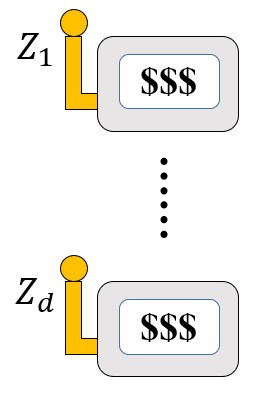
(a)

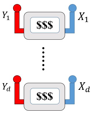
(b)

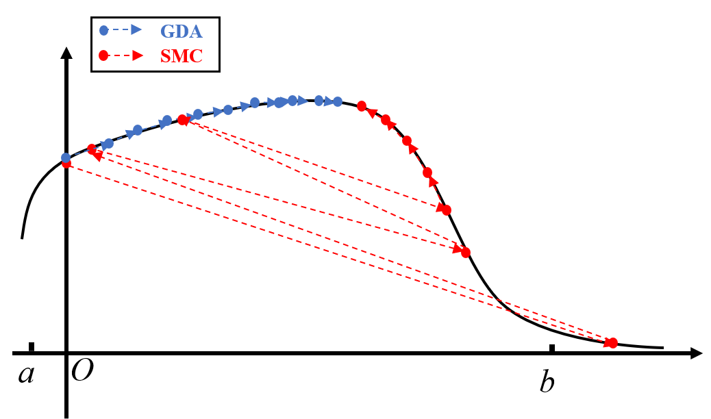
(c)

Figure 1: (a). Classic Monte Carlo sampling from a sequence of one-armed slot machines, whose arm have population $\{Z_{1},\cdots,Z_{d}\}$; (b). Strategic Monte Carlo sampling from a sequence of two-armed slot machines, whose arms populations $\{X_{1},\cdots,X_{d}\}$ and $\{Y_{1},\cdots,Y_{d}\}$; (c) The iterative mechanism for attaining the extreme value by the gradient descent ascent (blue arrow line) and SMCO (red arrow line) under $d=1$, where red points denote the iterative value $S_{m-1}^{\bm{\theta}^{*}}/(m-1)$ for SMCO.

Next, we use $d$ two-armed bandit model to characterize the proposed strategic Monte Carlo’s sampling process by denoting a sampling strategy by $\bm{\theta}=(\bm{\vartheta}_{1},\cdots,\bm{\vartheta}_{i},\cdots)$, where $\bm{\vartheta}_{i}=(\vartheta_{i1},\cdots,\vartheta_{id})$ and $\vartheta_{ij}=1$ (respectively, $\vartheta_{ij}=0$) means the $j{\rm th}$ component of the $i{\rm th}$ sample comes from arm $X_{j}$ with mean $\overline{\mu}_{j}$ (respectively, $Y_{j}$ with mean $\underline{\mu}_{j}$). Let $\{\bm{Z}_{i}^{\bm{\theta}}=(Z_{i1}^{\bm{\theta}},\cdots,Z_{id}^{\bm{\theta}}):i\geq 1\}$ given in [2.2] below be the $d$-dimensional samples obtained with the strategy $\bm{\theta}$. If $\bm{\theta}=(\bm{1},\bm{1},\cdots)$, that is, all samples are obtained from $(X_{1},\cdots,X_{d})$, then, by the classical law of large numbers, we know that the sample means $S_{n}^{\bm{\theta}}/n$ of $\{\bm{Z}_{i}^{\bm{\theta}}\}$ converges to $(\overline{\mu}_{1},\cdots,\overline{\mu}_{d})$, which the mean of $(X_{1},\cdots,X_{d})$, almost surely. However, it is difficult for most strategies to determine whether the sample mean $S_{n}^{\bm{\theta}}/n$ will converge to or might not converge at all. For any continuous real-valued function $f$, thanks to the nonlinear law of large numbers of bandit problems (see Theorem 2.1 below), we can show the limit behavior of $S_{n}^{\bm{\theta}}/n$ as follows:

$$\sup_{x\in\Gamma}f(x)=\lim_{n\to\infty}\sup_{\bm{\theta}\in\Theta}E\left[f\left(\frac{S_{n}^{\bm{\theta}}}{n}\right)\right],$$ [2.1]

where $\Gamma=[\underline{\mu}_{1},\overline{\mu}_{1}]\times\cdots\times[\underline{\mu}_{d},\overline{\mu}_{d}]$, which implies that finite rectangular region $\Gamma$-based optimization problem is transformed into an infinite set $\Theta$-based issue of policy formulation for attaining the extreme value. And $\Theta$ could denote all kinds of sets of possible strategies, including either a random strategy set such as $\epsilon$-greedy, Softmax, upper confidence bound, Gittin index, and some Bayesian methods, or fixed strategies such as playing the arm periodically by following a regular rule. This transformation from optimization problem to strategy development supplies a way to attain global optimality by engaging in the definition of all strategic sets of $\Theta$ because varying kinds of sets of $\Theta$ broadens the search space of optimal policies, provides flexibility, and facilitates learning via trial and error. More importantly, even for certain non-differentiable functions, the proposed strategic Monte Carlo method can still be applied to maximum optimization, as shown in the appendix.

Next, we will show a nonlinear law of large numbers of bandit problem to recast the challenging task of function global optimization into a bandit problem. For convenience, we begin with some basic settings and notations, which will also be applied in the rest of the paper. Let $(\Omega,\mathcal{F},P)$ be a discrete probability space. Consider $d$ two-armed bandit models, for $1\leq j\leq d$, assume that $(X_{j},Y_{j})$ denotes the random reward of one of these $d$ two-armed bandit models. Let $\{X_{i,j}:i\geq 1\}$ and $\{Y_{i,j}:i\geq 1\}$ respectively denote the outcomes from the arm $X_{j}$ and $Y_{j}$ at the $i{\rm th}$ round. A sampling strategy $\bm{\theta}$ is usually defined by a sequence of random vectors $\bm{\theta}=\{\bm{\vartheta}_{1},\cdots,\bm{\vartheta}_{n},\cdots\}$ where $\bm{\vartheta}_{i}=(\vartheta_{i1},\cdots,\vartheta_{id})$ and $\vartheta_{ij}=1$ (respectively, $\vartheta_{ij}=0$) means in the $i{\rm th}$ round we pull the arm $X_{j}$ (respectively, $Y_{j}$) of the $j{\rm th}$ slot machine. Let $\{\bm{Z}_{i}^{\bm{\theta}}=(Z_{i1}^{\bm{\theta}},\cdots,Z_{id}^{\bm{\theta}}):i\geq 1\}$ be a sequence of $d$-dimensional random vectors denote the $i{\rm th}$ reward obtained from these $d$ slot machines related to the strategy $\bm{\theta}$. That is, for $j=1,\cdots,d$,

$$Z_{ij}^{\bm{\theta}}=\left\{\begin{array}[]{ll}X_{i,j},&\text{ if }\ \vartheta_{ij}=1,\\ Y_{i,j},&\text{ if }\ \vartheta_{ij}=0.\end{array}\right.$$ [2.2]

We call a sampling strategy $\bm{\theta}=\{\bm{\vartheta}_{1},\cdots,\bm{\vartheta}_{n},\cdots\}$ admissible if $\bm{\vartheta}_{n}$ is $\mathcal{H}_{n-1}^{\bm{\theta}}$-measurable for all $n\geq 1$, where

$$\mathcal{H}_{n-1}^{\theta}=\sigma\{\bm{Z}_{1}^{\bm{\theta}},\cdots,\bm{Z}_{n-1}^{\bm{\theta}},\bm{\vartheta}_{1},...,\bm{\vartheta}_{n-1}\}\text{ for }n>1\text{, and }\mathcal{H}_{0}^{\bm{\theta}}=\{\emptyset,\Omega\}\text{.}$$

The set $\Theta$ denotes the collection of all admissible sampling strategies. For convenience, we assume that $\{X_{j}:1\leq j\leq d\}$ and $\{Y_{j}:1\leq j\leq d\}$ satisfy that

$$X_{j}=\mu_{X,j}+\xi,\quad Y_{j}=\mu_{Y,j}+\xi,$$ [2.3]

where $\xi$ is a bounded random variable with mean $0,$ variance $\sigma^{2}$ and bounded by $\delta>0$ (That is, $|\xi|<\delta$). Here $\mu_{X,j},\mu_{Y,j}\in\mathbb{R}$ are the means of $\{X_{j}:1\leq j\leq d\}$ and $\{Y_{j}:1\leq j\leq d\}$.

We will focus on the global optimization of a function $f$ on a bounded rectangular region $\Gamma$,

$$\Gamma:=[\underline{\mu}_{1},\overline{\mu}_{1}]\times[\underline{\mu}_{2},\overline{\mu}_{2}]\times\cdots\times[\underline{\mu}_{d},\overline{\mu}_{d}]\subset\mathbb{R}^{d}.$$ [2.4]

For the sake of rigor in the statement and proof of the theorem, we assume that the function $f$ is well-defined on the extension region $\Gamma_{\delta}$ of $\Gamma$,

$$\Gamma_{\delta}:=[\underline{\mu}_{1}-\delta,\overline{\mu}_{1}+\delta]\times[\underline{\mu}_{2}-\delta,\overline{\mu}_{2}+\delta]\times\cdots\times[\underline{\mu}_{d}-\delta,\overline{\mu}_{d}+\delta].$$ [2.5]

where $\delta$ is the bound of $\xi$ in [2.3].

Theorem 2.1 (A Unified Bandit Framework for Optimization).

Let $\Gamma$ and $\Gamma_{\delta}$ be the bounded rectangular regions on $\mathbb{R}^{d}$, given in [2.4] and [2.5]. Let $f$ be any continuous function defined on $\Gamma_{\delta}$ satisfied the growth condition, that is, there exists $p\geq 1$ such that $|f(x)|\leq c(1+\|x\|^{p-1})$, $x\in\Gamma_{\delta}$.Assume that the $d$ two-armed bandit models $\{(X_{j},Y_{j}):1\leq j\leq d\}$ satisfy that $\{\mu_{X,j},\mu_{Y,j}\}=\{\underline{\mu}_{j},\overline{\mu}_{j}\}$ for $1\leq j\leq d$, then the global optimization of $f$ on $\Gamma$ is equivalent to the problem of asymptotically maximizing the “bandit reward” with $f$

$$\sup\limits_{x\in\Gamma}f(x)=\lim\limits_{n\rightarrow\infty}\sup_{\bm{\theta}\in\Theta}E\left[f\left(\frac{S_{n}^{\bm{\theta}}}{n}\right)\right],$$ [2.6]

which can also be characterized by the bandit problem language,

$$\lim\limits_{n\rightarrow\infty}\inf_{\bm{\theta}\in\Theta}R_{f}^{\bm{\theta}}(n)=0,$$ [2.7]

where $R_{f}^{\bm{\theta}}(n)$ is the “averaged regret” with $f$ under $\bm{\theta}$,

$$R_{f}^{\bm{\theta}}(n)=\sup_{x\in\Gamma}f(x)-E\left[f\left(\frac{S_{n}^{\bm{\theta}}}{n}\right)\right].$$

Theorem 2.1 implies that the global optimization problem of the $d$-dimensional function $f$ on region $\Gamma$ now is transformed into $d$ (parallel) two-armed bandit problems. One just needs to find an asymptotically optimal strategy $\bm{\theta}^{*}$ such that

$$\lim\limits_{n\rightarrow\infty}R_{f}^{\bm{\theta}^{*}}(n)=0.$$

When $f(x)=x$, it degenerates to the classical bandit problem.

2.2 Algorithm: Strategic Monte Carlo

For “hill climbing for the blind” we turn to just use the sign information of derivative function by introducing an optimal strategy $\bm{\theta}^{*}$ to attain the local optimality under one kind of set $\Theta$ by just using the sign information of the derivative function in the fixed rectangular region $\Gamma$. In detail, if a strategy $\bm{\theta}^{*}$ can be given to make $f(S_{n}^{\bm{\theta}^{*}}/n)$ converge to one of maximums of $f$, it is also equivalent to giving a strategic Monte Carlo method to approximate the maximum points of the function $f$ on the region $\Gamma.$ With the assumption that the means of these two arms are known, we find that such strategy $\bm{\theta}^{*}=(\bm{\vartheta}_{1}^{*},\cdots,\bm{\vartheta}_{m}^{*},\cdots)$ can be constructed as follows: $\bm{\vartheta}_{m}^{*}=(\vartheta_{m1}^{*},\cdots,\vartheta_{md}^{*})$ and

$$\vartheta_{mj}^{*}=\left\{\begin{array}[]{cc}1,&\text{ if }\partial_{x_{j}}f\left(\frac{S_{m-1}^{\bm{\theta}^{*}}}{m-1}\right)\geq 0,\\ 0,&\text{ if }\partial_{x_{j}}f\left(\frac{S_{m-1}^{\bm{\theta}^{*}}}{m-1}\right)<0.\end{array}\right.$$ [2.10]

Intuitively, suppose the current sample mean is in a region where the function is increasing. In that case, we aim to maximize this sample mean by selecting a sample from a higher-mean arm (population) in the next round. Conversely, if the sample mean is in a region where the function is decreasing, we select from a lower-mean arm. Figure 1(c) shows the different iterative mechanisms for attaining the extreme value by the gradient descent ascent (blue arrow line) and SMCO (red arrow line) respectively. We also demonstrate that under the optimal strategy $\bm{\theta}^{*}$ for a given function $f$, the sample average $S_{n}^{\bm{\theta}^{*}}/n$ converges to the maximum point of $f$. This result constitutes the Strategic Law of Large Numbers for the bandit problem (Theorem 2.2 below). In the one-dimensional setting, our proposed two-armed bandit process devises strategies that combine the two arms with known distributions to identify the maximum value of a non-convex function $f$. This approach differs from the classical two-armed bandit model, which explores optimal arms to achieve the maximum average reward for each arm under a monotonic function $f$ with unknown distributions.

1 Input: Function $f$, Accuracy $\varepsilon$, Sample sums: $S_{1}^{\bm{\theta}}=0\in\mathbb{R}^{d}$.

2 Output: $f\left(\frac{S_{n}^{\bm{\theta}}}{n}\right)$.

3

4for $n=1$ to $\infty$ do

5    for $j=1$ to $d$ do

6      

7      if $\partial_{x_{j}}f\left(\frac{S_{n}^{\bm{\theta}}}{n}\right)\geq 0$ then

8          Draw sample from arm $X_{j}$ (larger mean) ;

9       end if

10      else

11          Draw sample from arm $Y_{j}$ (smaller mean);

12       end if

13      

14      Allocate the current component $Z_{n+1,j}^{\bm{\theta}}$ in [2.2].

15    end for

16   

17   Update $\bm{Z}_{n+1}^{\bm{\theta}}=(Z_{n+1,1}^{\bm{\theta}},\cdots,Z_{n+1,d}^{\bm{\theta}})~,~~S_{n+1}^{\bm{\theta}}=S_{n}^{\bm{\theta}}+\bm{Z}_{n+1}^{\bm{\theta}}$.

18 end for

19end for if $\left|f\left(\frac{S_{n}^{\bm{\theta}}}{n}\right)-f\left(\frac{S_{n+1}^{\bm{\theta}}}{n+1}\right)\right|\leq\varepsilon$.

Algorithm 1 SMCO: Strategic Monte Carlo Optimization

According to the idea in Figure 1, and with the Strategic Law of Large Numbers (Theorem 2.2) providing the theoretical guarantee, for any finite rectangular region $\Gamma$ in $\mathbb{R}^{d}$ and any continuous differential function $f$ on $\Gamma_{\delta}$, one can construct two sequences of populations $\{X_{1},\ldots,X_{d}\}$ and $\{Y_{1},\ldots,Y_{d}\}$ with means $\{\overline{\mu}_{1},\ldots,\overline{\mu}_{d}\}$ and $\{\underline{\mu}_{1},\ldots,\underline{\mu}_{d}\}$, respectively. Applying the optimal strategy $\bm{\theta}^{*}$ defined in Theorem 2.2 to obtain the samples $\{\bm{Z}_{i}^{\bm{\theta}^{*}}:i\geq 1\}$, we have the following, if $f$ has a unique extremum within the region $\Gamma$.

$$\sup_{x\in\Gamma}f(x)\approx f\left(\frac{S_{n}^{\bm{\theta}^{*}}}{n}\right),\quad P\text{-a.s.}.$$

The following theorem establishes the strategic law of large numbers of bandit problems, under the assumption that the means of these $2\times d$ arms are known. This theorem ensures that the sample mean $S_{n}^{\bm{\theta}^{*}}/n$, under the optimal strategy $\bm{\theta}^{*}$, converges to the global maximum point of $f$, if $f$ possesses a unique extremum within the region $\Gamma$, or alternatively, converges to one of the maximum points of $f$ in cases where multiple extrema exist within the region $\Gamma$.

Theorem 2.2 (Consistent Convergence).

Assume that these $2\times d$ arms have known means with $\mu_{X,j}=\overline{\mu}_{j},\mu_{Y,j}=\underline{\mu}_{j}$ for $j=1,\cdots,d$. Let $f$ be a continuous differential function on $\Gamma_{\delta}$, and satisfy

(A.1) : For any $i=1,\cdots,d$, $K_{i}\in\mathbb{N}$ is a fixed number, there exists two sets of points $c_{i}^{1}<\cdots<c_{i}^{K_{i}}\in[\underline{\mu}_{i},\overline{\mu}_{i}]$ and $b_{i}^{1}<\cdots<b_{i}^{K_{i}-1}\in[\underline{\mu}_{i},\overline{\mu}_{i}]$, such that the $i{\rm th}$ component of $f$ is increasing on $(b_{i}^{j-1},c_{i}^{j})$ for $j=1,\cdots,K_{i}$ with $b_{i}^{0}=\underline{\mu}_{i}-\delta$, and decreasing on $[c_{i}^{j},b_{i}^{j})$ for $j=1,\cdots,K_{i}$ with $b_{i}^{K_{i}}=\overline{\mu}_{i}+\delta$, that is, for any fixed $x=(x_{1},\cdots,x_{d})\in\Gamma_{\delta}$, the function $f(x_{1},..,x_{i-1},\cdot,x_{i+1},..,x_{d})$ is increasing on $(b_{i}^{j-1},c_{i}^{j})$ and decreasing on $[c_{i}^{j},b_{i}^{j})$ for $j=1,\cdots,K_{i}$.

(A.2) : For any $j=1,\cdots,d$, $\underline{\mu}_{j}+\delta<c_{j}^{1}$ and $\overline{\mu}_{j}-\delta>c_{j}^{K_{j}}$.

Let $\mathcal{M}$ denote all maximum points of $f$ on $\Gamma$, that is,

$$\mathcal{M}=\left\{(c_{1}^{j_{1}},\cdots,c_{d}^{j_{d}}):1\leq j_{1}\leq K_{1},\cdots,1\leq j_{d}\leq K_{d}\right\}.$$

Consider the strategy $\bm{\theta}^{*}=(\bm{\vartheta}^{*}_{1},\cdots,\bm{\vartheta}_{m}^{*},\cdots)$ where $\bm{\vartheta}_{m}^{*}=(\vartheta^{*}_{m1},\cdots,\vartheta_{md}^{*})$ is defined by

$$\vartheta_{mi}^{*}=\left\{\begin{array}[]{rl}1,&\text{if }\partial_{x_{i}}f\left(\frac{S_{m-1}^{\bm{\theta}^{*}}}{m-1}\right)\geq 0;\\ 0,&\text{otherwise},\end{array}\right.\quad i=1,\cdots,d.$$ [2.11]

Then one have

$$P\left(\lim_{n\to\infty}\frac{S_{n}^{\bm{\theta}^{*}}}{n}\in\mathcal{M}\right)=1.$$ [2.12]

Remark 2.1.

In our model, when these two arms (populations) coincide, our developed nonlinear and strategic law of large numbers (LLN) (Theorems 2.1 and 2.2) degenerates into the classical LLN, which serve as the theoretical foundation for the classical Monte Carlo method. Consequently, at a cursory glance, we can derive the following viewpoints: repeatedly operating a single-armed bandit corresponds to the conclusions drawn from the classical laws of large numbers, and can thus be utilized for simulating the integration of functions. However, strategically operating a two-armed bandit aligns with our proposed strategic laws of large numbers, enabling its application in simulating the extremum of functions.

Remark 2.2.

Here we make an assumption about the smoothness of the function $f$. In fact, the above conclusion can be obtained similarly for continuous function $f$ which is not differentiable. One can just approximate it by a smooth function, for example, $f_{\varepsilon}(x)=\int f(x+\varepsilon y)\phi(y)dy\to f(x),$ as $\varepsilon\to 0$, where $\phi$ is the probability density function of a standard normal distribution. Then, one can simulate the extremes of $f$ by applying the method to $f_{\varepsilon}$ for a small enough $\varepsilon$. In Subsection 2.2.4, we also give another way, which is based on a class of partial differential equations, to construct an optimal strategy to find the maximum value of the not differentiable function.

Inspired by the convergence rate of Peng’s nonlinear law of large numbers under the sublinear expectations (Fang et al, 2019 and Hu et al., 2021), in the last theorem of this subsection, we give the convergence rate of our strategic law of large numbers for bandit problems.

Theorem 2.3 (Convergence Rate).

Let $f$ be a continuous twice-differential function on $\Gamma_{\delta}$, and assume that $f$ has an unique maximum point $x^{*}=(x_{1}^{*},\cdots,x_{d}^{*})$ on $\Gamma$, and further the $i{\rm th}$ component of $f$ is increasing on $(\underline{\mu}_{i}-\delta,x_{i}^{*})$ and decreasing on $[x_{i}^{*},\overline{\mu}_{i}+\delta)$. Then we have,

$$\left|E\left[f\left(\frac{S_{n}^{\bm{\theta}^{*}}}{n}\right)\right]-f(x^{*})\right|\leq\max\left\{\frac{L_{f}\sigma\sqrt{d}}{\sqrt{n}},\frac{K_{f}\left(d\sigma^{2}+\sum_{j=1}^{d}(\overline{\mu}_{j}-\underline{\mu}_{j})^{2}\right)}{n}\right\},$$ [2.13]

where $L_{f}$ is the Lipschitz constant of $f$, $K_{f}=\max_{i,j}\sup_{x\in\Gamma_{\delta}}|\partial_{x_{i}x_{j}}^{2}f(x)|$ and $\sigma^{2}$ is the uniform variances of $\{X_{j}\}$ and $\{Y_{j}\}$ defined in [2.3]. Moreover,

$$E\left[\left\|\frac{S_{n}^{\bm{\theta}^{*}}}{n}-x^{*}\right\|^{2}\right]\leq\frac{d\sigma^{2}+\sum_{j=1}^{d}(\overline{\mu}_{j}-\underline{\mu}_{j})^{2}}{n}.$$ [2.14]

2.3 Strategic Monte Carlo Optimization with Tree Search for Global Optimization

This section introduces a tree search rule for SMCO to attain the global maximum of functions with multiple extrema by using a structure similar to Monte Carlo Tree Search(MCTS), a well-known technique in complex environments like the game of AlphaGo. MCTS has been successfully used in Go, known for its ability to effectively escape local optima and achieve global optimal solutions in complex game environments; see, e.g., Gelly et al. (2006) and Browne et al. (2012). By simulating games and iteratively expanding the search tree, MCTS effectively balances exploration and exploitation, making it a crucial technique for navigating Go’s vast search space and developing optimal strategies even with incomplete information.

In this paper, we apply MCTS to complex function optimization framework, demonstrating its effectiveness beyond traditional optimization methods. Because MCTS explores all kinds of strategy sets $\Theta$ by continually changing the subregions of the whole rectangular region $\Gamma$ during the iterations, meaning that various subregions of $\Gamma$ correspond to the evolving $\Theta$ for ensuring the global optimality. Specifically, our SMCO with Tree Search will explore nodes that enable the SMCO to converge to the global maximum. Figure 2 presents the detailed steps of the SMCO with Tree Search and the role of each step is shown below.

Selection: In each iteration, beginning from the root node $s_{0}$, the best child node is selected and designated as the new parent node. This process continues recursively until a node without children is reached. The selection criterion is based on the node value $Q$ and the number of explorations $N$. The initial node value $Q=Q_{0}$, and $Q_{0}$ is defined as the maximum value of $f(x)$ that converges from the coordinate of that node using the SMCO algorithm. The method of updating the node value can be referred to Algorithm 2. If the parent node is $s$, its best child node is defined as

$$\underset{v\in\text{children of }s}{\text{argmax}}{Q(v)}+C\sqrt{\frac{\log N(s)}{N(v)}},$$ [2.15]

where $C$ denotes exploration weight.

Expansion: If the selected node has been explored at least once, it is expanded to generate new child nodes. The first new child node then undergoes rollout in the next step. If the number of explorations for this child node is zero, it directly proceeds to the rollout step.

Rollout: Performing a rollout on a node involves starting from the coordinates corresponding to the node, using the SMCO algorithm to compute the maximum value, and adding it to the node value.

Backpropagation: Backpropagation updates a node’s value and the number of explorations, then propagates these updates to its parent node, continuing this process until the root node is reached.

Figure 2: The algorithmic flowchart of strategic Monte Carlo Optimization with tree search for finding the global maximum.

Theorem 2.2 implies that SMCO algorithm samples from $n=1$, but if SMCO samples from some $N$, meaning for an ${x}$ and a strategy ${\bm{\theta}}_{N}=(\bm{\vartheta}_{1},\bm{\vartheta}_{2},\ldots,\bm{\vartheta}_{N})$ that satisfies ${S_{N}^{{\bm{\theta}}_{N}}}/{N}={x}$, The conclusion in the Theorem 2.2 still holds. Denoting $\bm{\theta}^{\prime}=(\bm{\vartheta}_{1},\ldots,\bm{\vartheta}_{N},\bm{\vartheta}_{N+1}^{*},\ldots)$, we also have

$$P\left(\lim_{n\to\infty}\frac{S_{n}^{\bm{\theta}^{\prime}}}{n}\in\mathcal{M}\right)=1.$$ [2.16]

The above explanation implies that when MCTS explores a new node, it is guaranteed that the convergence value obtained from that node using the SMCO algorithm must be a maximum value of $f(x)$.

Theorem 2.4 (Global Optimality).

Let $f$ be a continuous differential function on $\Gamma_{\delta}$ and satisfy Conditions (A.1) and (A.2), $s_{i}$ denotes the $i$th node searched in the Monte Carlo tree. Let $T_{n}=\underset{1\leq i\leq n}{\max}Q_{0}(s_{i})$, then we have:

$$P\left(\lim_{n\to\infty}T_{n}=\underset{x\in\Gamma}{\sup}f(x)\right)=1.$$ [2.17]

Remark 2.3.

Theorem 2.4 shows that as the number of explorations increases, the maximum value of $f(x)$ explored will converge to the global maximum value of $f(x)$. It is worth mentioning that for the case where there are multiple global maximum points, SMCO with tree search could search them all by simply recording the convergence coordinates of nodes during the iterations of SMCO algorithm and picking out the coordinates that correspond to the global maximum.

2.4 Strategic Monte Carlo Optimization with Partial Differential Equation for Global Optimization

In general, the function $f$ may not be differentiable or satisfy the assumption (A.1) or (A.2), in which case a sequence of asymptotically optimal strategies can be constructed using partial differential equation (PDE). For any small enough $\epsilon>0$, consider the PDE

$$\left\{\begin{array}[]{l}\displaystyle\partial_{t}u_{\epsilon}(t,x)+\sup_{p\in\Gamma}\left[D_{x}u_{\epsilon}(t,x)\cdot p\right]+\frac{\epsilon^{2}}{2}\textrm{tr}\left[D_{x}^{2}u_{\epsilon}(t,x)\right]=0,\quad(t,x)\in[0,1+\epsilon)\times\mathbb{R}^{d},\\ u_{\epsilon}(1+\epsilon,x)=\hat{f}(x),\end{array}\right.$$ [2.18]

where $\hat{f}$ is an extension of $f$ defined on $\mathbb{R}^{d}$ and $D_{x}u_{\epsilon},D_{x}^{2}u_{\epsilon}$ denote the gradient vector and the Hessian matrix of the function $x\to u_{\epsilon}(t,x)$. Then we will use the sign of the gradient vector $D_{x}u_{\epsilon}$ to construct a sequence of strategies such that $f(S_{n}^{\bm{\theta}}/n)$ approximate $\sup_{x\in\Gamma}f(x)$.

Theorem 2.5.

Let $f$ be a Lipschitz continuous function on $\Gamma_{\delta}$ with Lipschitz constant $L_{f}$, and $\hat{f}$ be a bounded Lipschitz continuous (with Lipschitz constant $L_{f}$) extension of $f$ defined on $\mathbb{R}^{d}$. For any $\epsilon>0$ and $n\in\mathbb{N}$, the strategy $\hat{\bm{\theta}}^{n,\epsilon}=(\hat{\bm{\vartheta}}_{1}^{n,\epsilon},\cdots,\hat{\bm{\vartheta}}_{i}^{n,\epsilon},\cdots)$, where $\hat{\bm{\vartheta}}_{i}^{n,\epsilon}=(\hat{\vartheta}_{i1}^{n,\epsilon},\cdots,\hat{\vartheta}_{id}^{n,\epsilon})$, is defined by

$$\hat{\vartheta}_{ij}^{n,\epsilon}=\left\{\begin{array}[]{cc}1,&\displaystyle\textup{ if }\partial_{x_{j}}u_{\epsilon}\left(\frac{i}{n},\frac{S_{i-1}^{\hat{\bm{\theta}}^{n,\epsilon}}}{n}\right)>0,\\ 0,&\textup{otherwise}.\end{array}\right.,\text{ for }1\leq i\leq n,\text{ and }\hat{\vartheta}_{ij}^{n,\epsilon}=1\text{ for }i>n$$ [2.19]

where $u_{\epsilon}$ is the unique solution of PDE [2.18]. Then $\{\hat{\bm{\theta}}^{n,\epsilon}\}$ is asymptotically $\epsilon$-optimal in the since that

$$\limsup_{n\to\infty}\left|E\left[f\left(\frac{S_{n}^{\hat{\bm{\theta}}^{n,\epsilon}}}{n}\right)\right]-\sup_{x\in\Gamma}f(x)\right|\leq L_{f}\epsilon(2+\sqrt{\epsilon}+\sqrt{1+\epsilon})+C\epsilon^{2},$$ [2.20]

where $C$ is constant depend on $f$.

Remark 2.4.

To construct a sequence of asymptotically $\epsilon$-optimal strategies, we only need to know the sign of each component of the gradient vector $D_{x}u_{\epsilon}$. For some special terminal conditions $\hat{f}$, the sign of the gradient vector $D_{x}u_{\epsilon}$ is easy to known.

For example, when $f$ is differential on $\Gamma_{\delta}$ and only has one extreme $x^{*}=(x_{1}^{*},\cdots,x_{d}^{*})$ (which is the global maximum point) and satisfies condition (A.1) with $K_{i}=1$ for $i=1,\cdots,d$. It can be checked that the sign of the gradient vector $D_{x}u_{\epsilon}$ is same as the sign of the gradient vector $D_{x}f$, that is,

$$\left\{\partial_{x_{j}}u_{\epsilon}\left(\frac{i}{n},\frac{S_{i-1}^{\hat{\bm{\theta}}^{n,\epsilon}}}{n}\right)>0\right\}\text{ is equivalent to }\left\{\partial_{x_{j}}f\left(\frac{S_{i-1}^{\hat{\bm{\theta}}^{n,\epsilon}}}{n}\right)>0\right\}.$$

3 Numerical Comparisons

The following numerical studies compare the performance of our proposed SMCO algorithm to that of several popular metaheuristic optimization methods, including the simulated annealing (SA) of Kirkpatrick et al. (1983) and the particle swarm optimization (PSO) of Eberhart and Kennedy (1995). we check their performances for attaining the global maximum by optimizing deterministic and random functions respectively. The other experimental studies are shown in the appendix through comparing SMCO and GDA’s performance in optimizing deterministic functions and set identification.

3.1 SMCO with tree search: optimizing deterministic functions for global maximum

This part considers various function formations, including different dimensions, single and multi-modal functions, especially the non-convex Rastrigin function with amounts of maximum points.

Case 1 (tall-narrow function): $f(x)=-0.006037x^{6}+0.2125x^{5}-2.946x^{4}+20.26x^{3}-71.23x^{2}+117.0x-63.98$, $x\in[1,10]$.

Case 2 (function with extremely near maxima): $f(x)=\sin(3x)+\sin(5x)-\frac{1}{1+20000x^{2}},x\in[-4,1]$, which combines two sine functions and a polynomial function with two extremely near maxima.

Case 3 (multivariate function): $f(x,y)=6-(x^{2}-2)^{2}-(y^{2}-2)^{2}-\frac{y}{200x+500},x\in[-2,2]$ and $y\in[-2,2]$, which is a multivariate function with two variables.

Case 4 (Rastrigin function): $f(x,y)=20+x^{2}+y^{2}-(10\cos(2\pi x)+10\cos(2\pi y)),x\in[-1.9,1.9]$ and $y\in[-1.9,1.9]$, which is a non-convex function with amounts of maximum points.

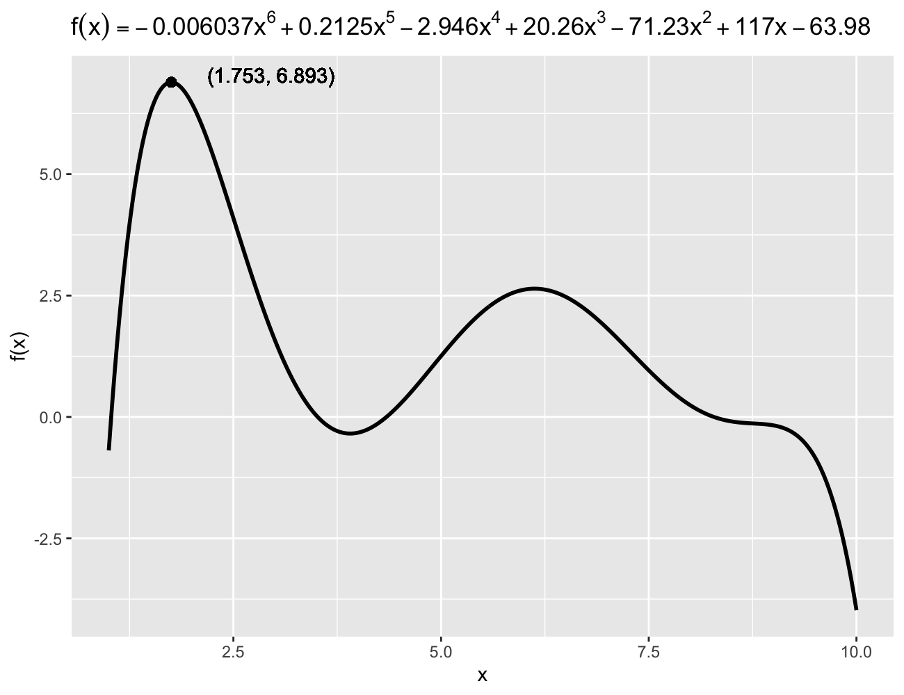
(a)

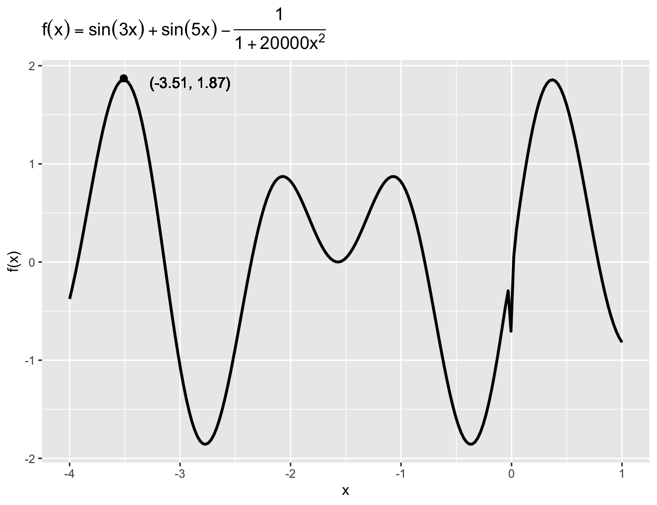
(b)

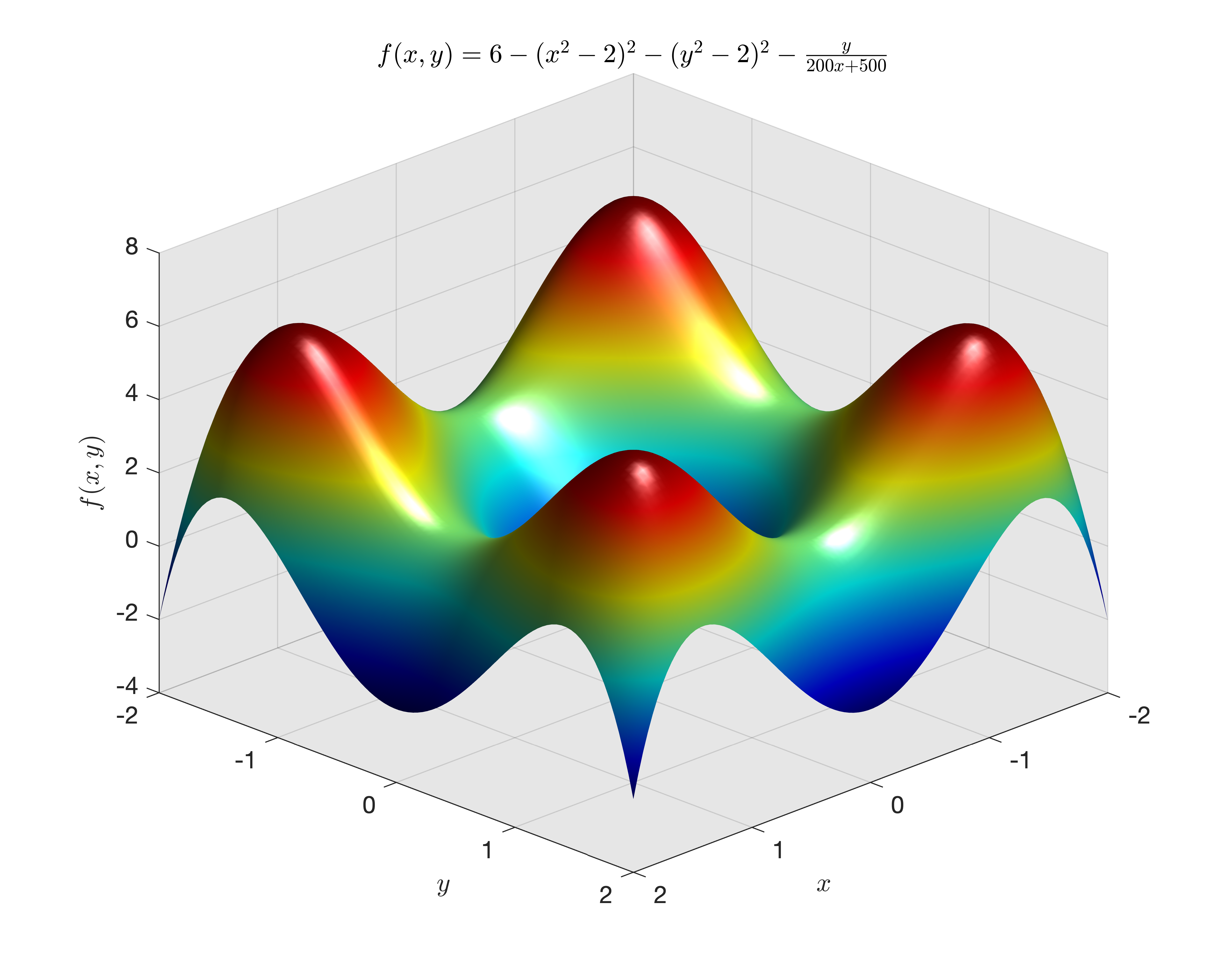
(c)

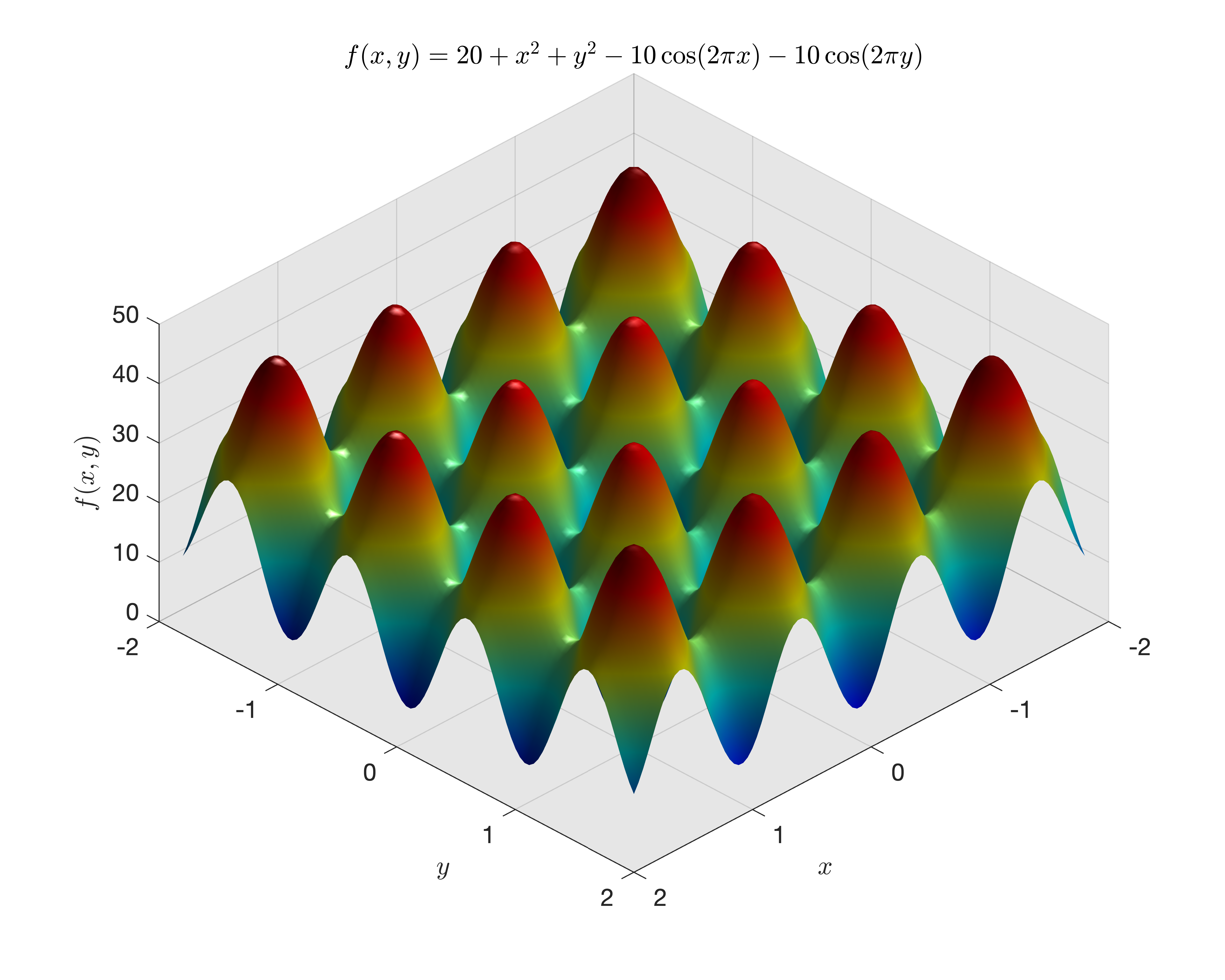
(d)

Figure 3: The function images correspond to the respective of Cases 1-4 in Subsection 3.1.

500 repeated experiments are conducted to identify the global maximum for the considered four functions above under SMCO with tree search, SA, and PSO, $\|x_{m}-x_{m-1}\|<1\times 10^{-7}$ is chosen as the stopping criterion. Given that the performance of SA is affected by the initial temperature $T$ and the performance of PSO is influenced by the number of particles $S$, we considered the initial temperature $T=80$ and $T=100$ for SA, as well as the particle numbers $S=100$ and $S=150$ for PSO in all cases. For SMCO with tree search, we use the number of explorations $N=50$ and the exploration weight $C=5$. The considered evaluation index “Accuracy” denotes the frequency of the convergence point attains the true global maximum among the 500 experimental replicates. Additionally, the average running time$\times 10^{2}$ after all repeated experiments is presented to check their operational efficiency.

All results are documented in Table 1 and imply that SMCO with tree search consistently finds the global maximum with high accuracy. In Case 1, both SMCO with tree search and PSO achieved the global maximum, with SMCO showing a slightly lower running time than PSO and significantly lower running time than SA. SMCO with tree search maintained high accuracy In Case 2 and PSO also performed well with slightly lower accuracy, but SA had lower accuracy and higher running time. For the multivariate function in Case 3, both SMCO with tree search and PSO perform well, which indicates that they pass the performance test, while they have a significant advantage in terms of speed over SA. For the Rastrigin function optimization in Case 4, SMCO with tree search continued to achieve the global maximum with higher accuracy and lower running time. PSO showed relatively reasonable performance, with some variation in accuracy based on the number of particles, whereas SA had the lowest accuracy and highest running time among the methods. Therefore, SMCO with tree search demonstrated high accuracy in finding the global optimal solution and incurred lower time costs.

Noting that the performance of SA algorithm is unsatisfactory for functions with multiple maximums (Case 1) or for functions with multiple similar maximums (Cases 2 and 4). The PSO algorithm demonstrates an advantage over SA algorithm in identifying functions with multiple maximums when there are large differences between them; however, it remains inadequate in distinguishing functions with closely maximums. In contrast, SMCO with tree search could efficiently and accurately identify the global maximum for functions with multiple maximum points, regardless of whether they are similar or not.

Table 1: Accuracy and running time of different optimization methods in finding the global maximum of different functions in Subsection 3.1. SMCO with tree search demonstrated higher accuracy with lower time costs.

Case		Method		Accuracy		Time$\times 10^{2}$
		SMCO with tree search		1.00		1.02
		SA($T=$ 80)		0.99		6.87
Case 1		SA($T=$ 100)		0.98		7.17
		PSO($S=$ 100)		1.00		2.21
		PSO($S=$ 150)		1.00		2.69
		SMCO with tree search		0.97		1.20
		SA($T$= 80)		0.87		6.29
Case 2		SA($T$= 100)		0.83		6.79
		PSO($S$= 100)		0.88		2.07
		PSO($S$= 150)		0.92		2.76
		SMCO with tree search		1.00		3.38
		SA($T$= 80)		0.97		20.35
Case 3		SA($T$= 100)		0.98		20.48
		PSO($S$= 100)		1.00		3.97
		PSO($S$= 150)		1.00		4.62
		SMCO with tree search		0.93		2.85
		SA($T$= 80)		0.65		14.07
Case 4		SA($T$= 100)		0.58		14.48
		PSO($S$= 100)		0.62		4.33
		PSO($S$= 150)		0.68		5.94

3.2 SMCO, PSO and SA: optimizing random functions

In this subsection, we compare the performance of our SMCO in optimizing two random functions to those of the PSO and SA methods.

Example 1 (Likelihood function with few samples): The log-likelihood surface for the Cauchy density function $\beta/\{\pi(\beta^{2}+(Z-x)^{2})\}$ is considerably difficult to optimize when estimating $x$ for some known fixed values of $\beta$ (Brooks and Morgan, 1995), where $Z$ and $x$ denote the random sample and unknown parameter of interest. Let the random samples be generated from $Z_{i}\in\{$-4.20, -2.85, -2.30, -1.02, 0.70, 0.98, 2.72, 3.50$\}$, then the log-likelihood can be written as $N\log\beta-\sum_{i=1}^{N}\log\left\{\beta^{2}+\left(Z_{i}-x\right)^{2}\right\}-N\log\pi$ and the maximum likelihood estimate for $x$ is the minimizer of

$$f(x)=\sum_{i=1}^{N}\log\left\{\beta^{2}+\left(Z_{i}-x\right)^{2}\right\}.$$

Example 2 (Multivariate regression model): We generate data from the linear regression model, $Y_{i}=Z_{i}^{\top}x+\varepsilon_{i},$ $i=1,\ldots,N,$ where $Z_{i}=(Z_{i1},\cdots,Z_{ip})$ is generated from a triple three-variate normal distribution with zero mean vector and covariance element $0.7^{i-j}$, and $\varepsilon_{i}$ is taken from the standard normal distribution. The coefficient estimator maximizes the following negative quadratic loss function:

$$f(x)=-\sum_{i=1}^{N}(Y_{i}-Z_{i}^{\top}x)^{2},p=5,N=20\;{\rm for}\;x=(1,3,1.5,1,-0.8)^{\top},$$

$$f(x)=-\sum_{i=1}^{N}(Y_{i}-Z_{i}^{\top}x)^{2}-N\lambda\|x\|,p=1000,N=200\;{\rm for}\;x=(1,3,1.5,1,-0.8,{\bf 0}_{p-5}^{\top})^{\top}.$$

For Example 1, Figure 4 depicts one thousand iterative points of Cauchy log-likelihood before attaining the global maximum point $(0.73,-5.36)$ under the three optimization algorithms: SA, PSO and our proposed SMCO. The depicted scatterplot of the Cauchy log-likelihood implies that our SMCO delivers faster exploration to reach the maximum point in terms of more accumulated points around the global maximum point. The SA algorithm required 2075.7 milliseconds, PSO took 3250.8 milliseconds, whereas our SMCO method consumed only 20 milliseconds.

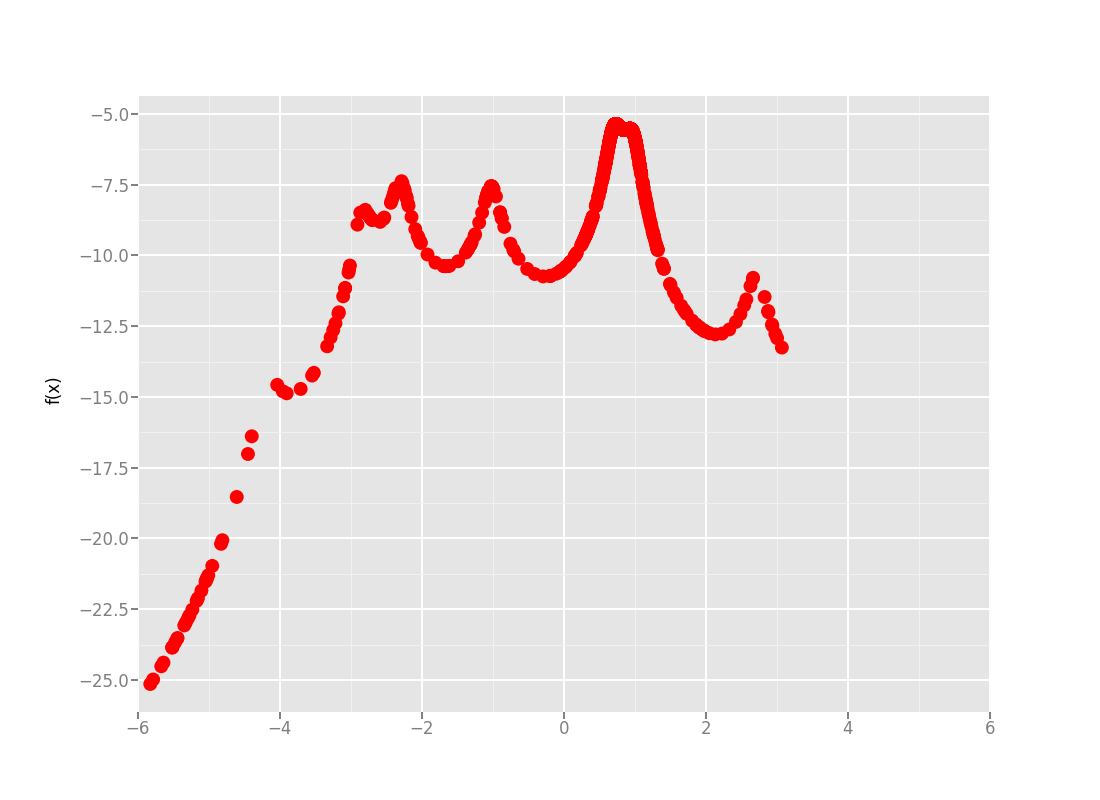
(a)

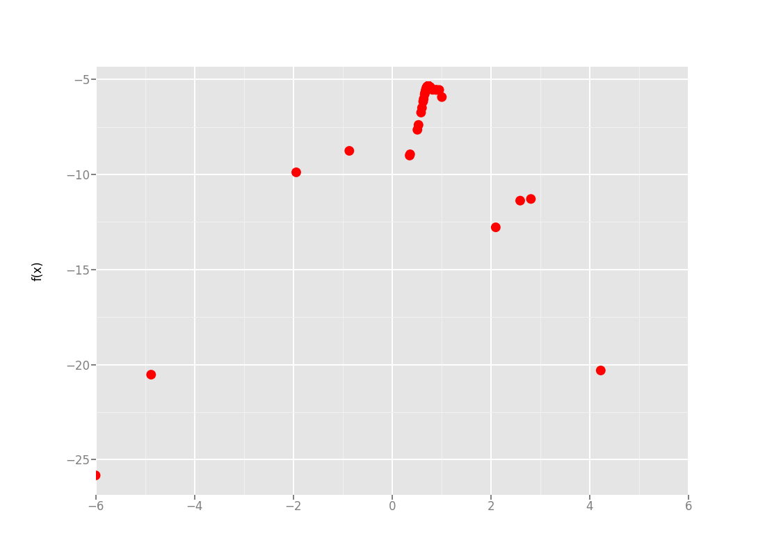
(b)

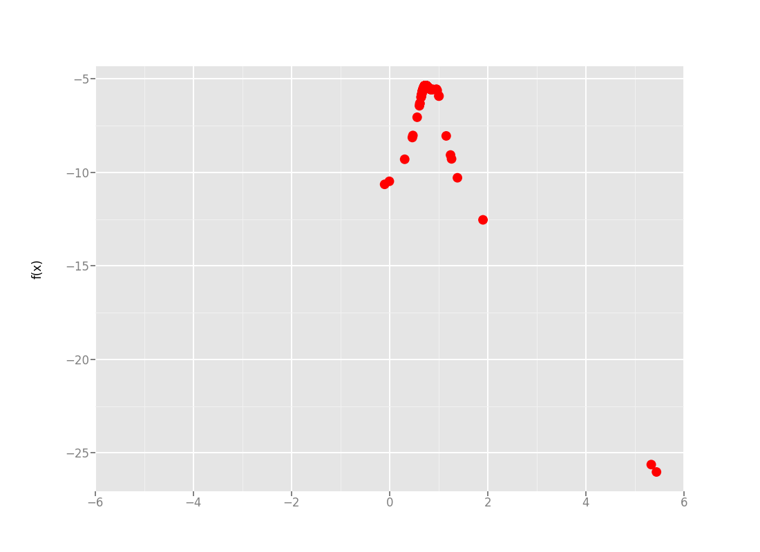
(c)

Figure 4: The iterative point-specific function values of Cauchy log-likelihood before attaining the true maximum solution $x^{*}=0.73$ in Example 1 under SA, PSO, and SMCO algorithms respectively, where the accuracy levels are set as under the accuracy levels $|f(x_{m})-f(x_{m-1})|<10^{-7}$ for the three optimizer.

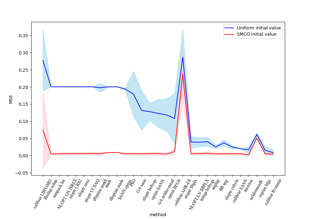
(a)

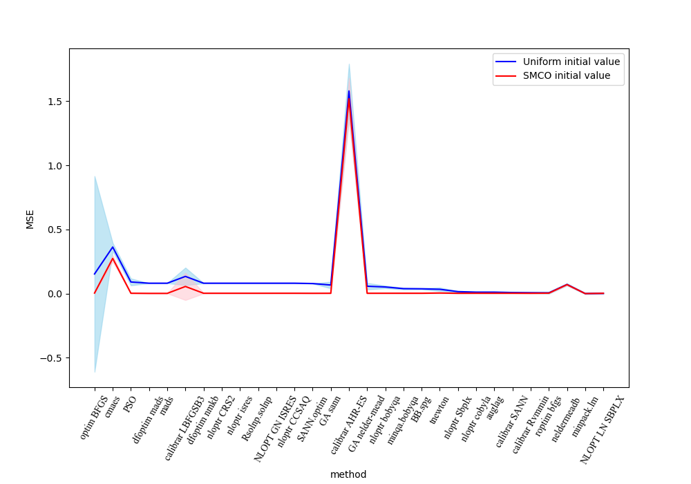
(b)

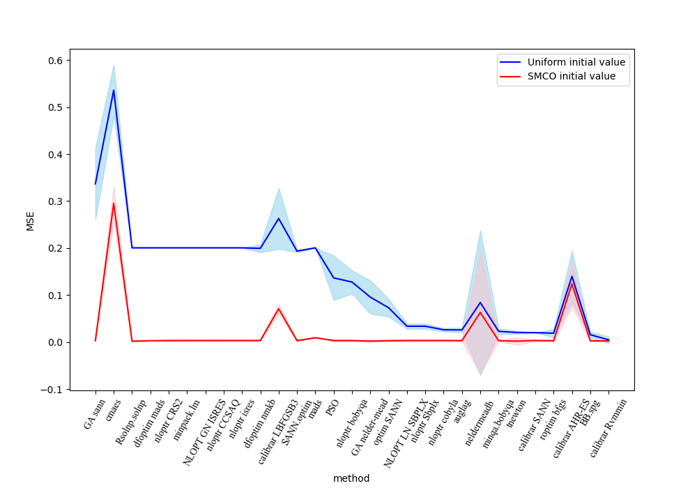
(c)

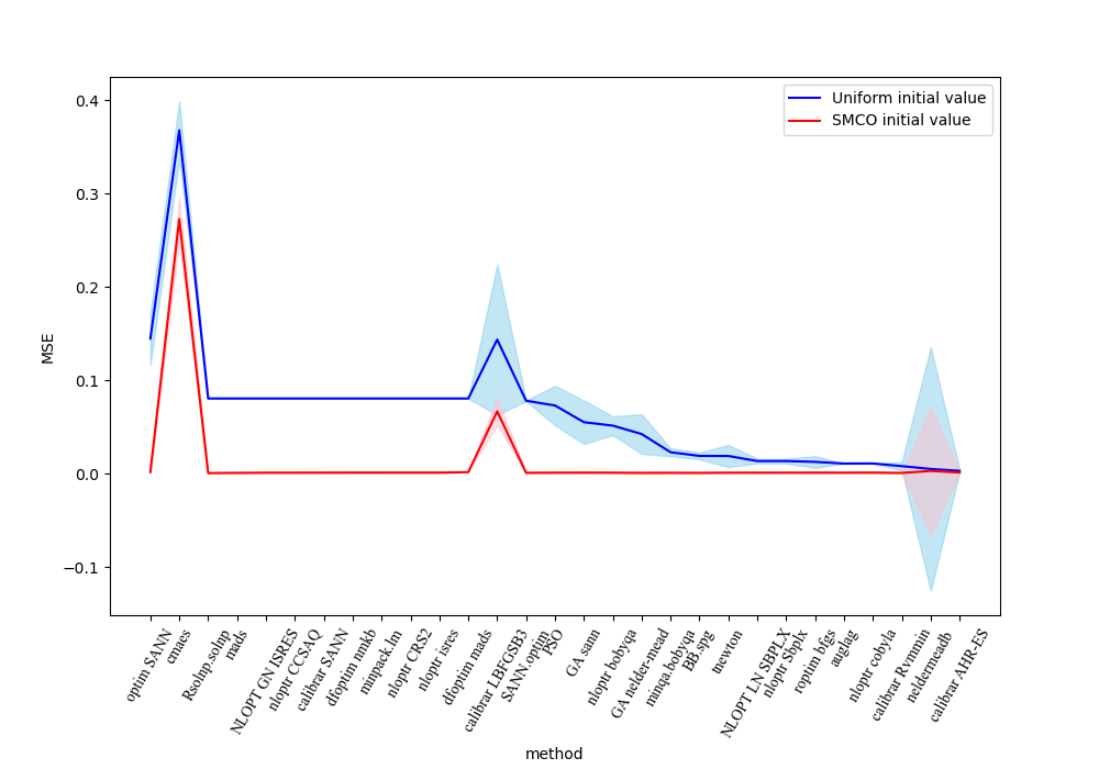
(d)

Figure 14: The means (the lines) and the standard errors (the shadows) of 500 MSEs across 30 optimization methods from https://cran.r-project.org/web/views/Optimization.html by using the iterative value of SMCO optimizer after 20 samplings as the initial value (the red lines and shadows) and uniform initial value vector $(0,\cdots,0)_{p}^{\top}$ (the blue lines and shadows) under four cases of sample sizes and dimensions for Multivariate regression model of Example 2.

For Example 2, Figure 5 presents the boxplots of the 500 mean square errors $\|x_{m}-x^{*}\|^{2}/p$ (MSE) and the running duration (Time) after 500 replicates with the low-dimensional (the left panel) and the high-dimensional (the right panel) regressions by using the PSO, SA, and SMCO algorithms, where the convergence value $x_{m}$ is attained under the accuracy levels $|f(x_{m})-f(x_{m-1})|<10^{-7}$ for the three considered optimization methods with initial value $(0.5,\cdots,0.5)_{p}^{\top}$ for SA, and SMCO algorithms, and the Time value in the high-dimensional case divides the true running duration by 100. Figure 5(a) shows that our SMCO algorithm with the left uniform distributions Unif(-4.5,-4) and right uniform distributions Unif(3.5, 4) for each variable component has the smallest MSE and the fastest running speed in terms of the smallest medians in the low-dimensional regression with left po, and the proposed SMCO optimizer spends a little more running time than SA method but obtains the smallest MSE for the high-dimensional case, as shown in Figure 5(b), where we use the iterative value of SMCO optimizer after 20 samplings, i.e., $x_{20}$ to determine the left uniform distribution Unif($x_{20}$-0.01, $x_{20}$) and right uniform distribution Unif($x_{20}$, $x_{20}$+0.01) for each variable component of the SMCO algorithm. Example 2 also serves to check the improved performance of the other 30 popular optimization methods from https://cran.r-project.org/web/views/Optimization.html by using the iterative value of SMCO optimizer after 20 samplings as the initial value, because the means of 500 MSEs across all optimization methods by using the SMCO initial value are smaller than those are obtained under the uniform initial value vector $(0,\cdots,0)_{p}^{\top}$ with red line being lower than the blue line in Figure 14. Meanwhile, the estimation performance of standard errors are also enhanced by using the SMCO initial values in terms of the narrower red shadow than the blue shadow.

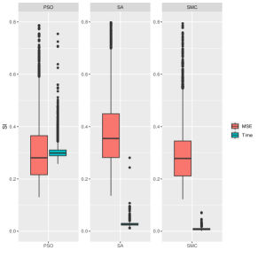
(a)

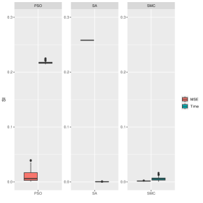
(b)

Figure 5: Boxplots of the mean square errors $\|x_{m}-x^{*}\|^{2}/p$ (MSE) and the running duration (Time) after 500 replicates in Example 2 with the low-dimensional (the left panel) and the high-dimensional (the right panel) regressions by using the PSO, SA, and SMCO algorithms, where the convergence value $x_{m}$ is attained under the accuracy levels $|f(x_{m})-f(x_{m-1})|<10^{-7}$ for the three considered optimization methods and the Time value in the right panel divides the true running duration by 200.

4 Real data analysis

The subjects of this real data were recruited from a community-based cross-sectional study from six communities in Chengdu and Ethics approval was obtained from the Chengdu First People’s Hospital and all participants were provided written informed consent before the questionnaire interviews. A comprehensive questionnaire including information on demographic and socioeconomic characteristics, personal and family medical history, and lifestyle risk factors was administered by trained interviewers. Anthropometric measurements, including height, and weight were taken using calibrated instruments with standard protocols, with participants wearing light clothing and bare feet. Blood samples were collected to test the serum concentrations, including glucose, triglyceride, total cholesterol, creatinine, uric acid, and high-density lipoproteins.

This study takes whether the participant suffers from hypertension or not as the categorical response variable $Y$, which is measured by systolic blood pressure (SBP) and diastolic blood pressure (DBP) with SBP and DBP being determined by using a digital sphygmomanometer (Omron HEM-907, Japan) three times after at least five minutes of rest in a seated position. Meanwhile, five variables including the age of participants ($Z_{1}$), whether suffering from chronic bronchitis or not ($Z_{2}$), serum-lipid including triglyceride (mmol/L, $Z_{3}$), total cholesterol (mmol/L, $Z_{4}$) and uric acid (umol/L, $Z_{5}$) are selected as the important predictors of hypertension by using the classical logistic regression under the significant level $0.1$. Let $Z=(1,Z_{1},\cdots,Z_{5})^{\top}$, this study considers the following objective function:

$$f(x)=-\frac{1}{N}\sum_{i=1}^{N}\left(Y_{i}-\frac{\exp(Z_{i}^{\top}x)}{1+\exp(Z_{i}^{\top}x)}\right)^{2},\;N=855.$$

$\begin{array}[]{lllll}\hline\cr\text{Variable}&\text{Data type }&\text{Value range}&\text{Variable meaning}\\ \hline\cr\text{Response variable}\;Y&\text{Discrete}&\{0,1\}&\text{suffering from hypertension or not}\\ \text{Explanatory variable}\;Z_{1}&\text{Continuous}&[20,98]&\text{the age of participants}\\ \text{Explanatory variable}\;Z_{2}&\text{Discrete}&\{0,1\}&\text{suffering from chronic bronchitis or not }\\ \text{Explanatory variable}\;Z_{3}&\text{Continuous}&[0.1,11.9]&\text{serum-lipid including triglyceride (mmol/L)}\\ \text{Explanatory variable}\;Z_{4}&\text{ Continuous}&[0.6,9.67]&\text{total cholesterol (mmol/L)}\\ \text{Explanatory variable}\;Z_{5}&\text{Continuous}&[3.78,688]&\text{uric acid (umol/L)}\\ \hline\cr\end{array}$

Figure 6 shows the converted function value (CFV) $-f(x_{m})$ across the iterative/sampling number $m$ (the left panel) or the varying accuracy levels $|f(x_{m})-f(x_{m-1})|<\varepsilon$ (the right panel) to stop the algorithms under the considered five optimization methods including SMCO, PSO, SA, SMCO$\_$SA and SMCO$\_$PSO, where SMCO$\_$SA and SMCO$\_$PSO treat the SMCO convergence value as the initial values of SA and PSO, which implies that (1) SMCO can attain the minimum converted function value faster than PSO, SA; (2) the converted function value $-f(x_{m})$ can attain the minimum after 5, 1 and 14 iterative numbers under SMCO, SMCO$\_$SA and SMCO$\_$PSO respectively (see Figure 6(a)); (3) SMCO$\_$SA and SMCO$\_$PSO also outperform the respective methods SA and PSO at the considered accuracy levels (see Figure 6(b)), because treating the SMCO convergence value as the initial value helps SA and PSO attain the minimum of converted function value faster.

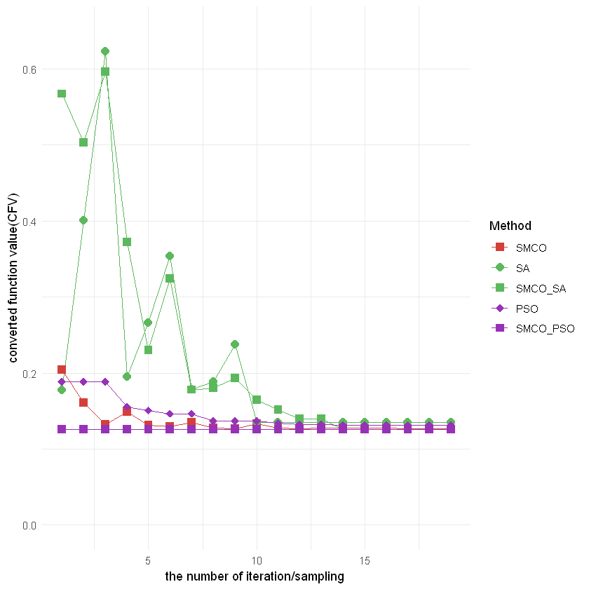
(a)

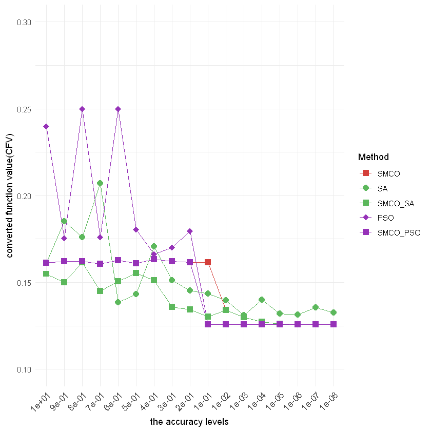
(b)

Figure 6: The converted function value (CFV) $-f(x_{m})$ across the iterative/sampling number $m$ (the left panel) or the varying accuracy levels $|f(x_{m})-f(x_{m-1})|<\varepsilon$ (the right panel) to stop the algorithms under the considered five optimization methods including SMCO, PSO, SA, SMCO$\_$SA and SMCO$\_$PSO, where SMCO$\_$SA and SMCO$\_$PSO treat the SMCO convergence value as the initial values of SA and PSO for the real data.

5 Conclusion

Through constructing a unified two-armed bandit framework for global optimization, this article transforms the optimizer search of general purpose optimization in a finite rectangle region to the optimal strategy formulation of multiple two-armed bandits model in infinite policy sets. By leveraging the strategic bandit process-driven optimization framework, we introduce the strategic Monte Carlo Optimization algorithm, which fills a research gap in the current Monte Carlo experimental design for global optimization of possibly multi-modal functions, which extends the application scope of the classic Monte Carlo algorithms designed for approximating integrals. Many optimization algorithms exist, such as the gradient descent ascent, the Newton-Gauss method, or the truncated Newton method. Not many global optimization algorithms have been shown to converge almost surely to the global solutions for general objective functions yet. Our proposed Strategic Monte Carlo Optimization (SMCO) algorithm with tree search is shown theoretically to attain global solutions faster and more accurately.

The developed SMCO is simple to implement and can readily generalize to higher-dimensional global optimization, which is not sensitive to the initial points and stepsizes. Although this development of a unified two-armed bandit framework for global optimization offers asymptotic convergence guarantees by the developed strategic law of large numbers, the address of finite sample complexity and total computation efforts will be further studied. Futhermore, the simulated results shows our SMCO algorithm has low computational complexity and fewer sampling numbers (corresponding to the iterative numbers), which looks like twice speed compared with classic gradient descent in the one-dimensional optimization and $2d$ times speed in the $d$ dimensions. Then another suggestion is that one could also combine our SMCO and other popular algorithms for various extensions as a quick explorer of initial value for other optimization methods.

Online content

All methods, additional references, nature research reporting summaries, supplementary information, acknowledgments, peer review information, details of author contributions and competing interests, and statements of data and code availability are available online.

Bandit framework for non-differentiable functions

Figure 8 presents two examples of using a bandit framework to optimize non-differentiable functions.

• Example 1: Sum of triangular wave functions. Consider a triangular wave function $f_{1}(x)$ on [0, 1]. Divide $f_{1}(x)$ into 4 parts and reduce its height to 1/2 to obtain function $f_{2}(x)$. Divide $f_{1}(x)$ into $4^{2}$ parts and reduce its height to 1/3 to obtain $f_{3}(x)$ (as shown in Figure 7), and $f_{4}(x)$ and $f_{5}(x)$ have similar generation processes. Finally, add $f_{1}(x),f_{2}(x),\ldots,f_{5}(x)$ together to obtain the function $f(x)$ (as shown in Figure 8(a)). Since $f(x)$ is non-differentiable at many points, traditional derivative-based optimization methods are ineffective, yet strategic Monte Carlo method can still provide an optimal strategy $\bm{\theta}^{*}=(\bm{\vartheta}_{1}^{*},\bm{\vartheta}_{2}^{*},\bm{\vartheta}_{3}^{*},\ldots)$, where $\bm{\vartheta}_{5i+1}^{*}=1,\bm{\vartheta}_{5i+2}^{*}=1,\ldots,\bm{\vartheta}_{5i+4}^{*}=1$ and $\bm{\vartheta}_{5i+5}^{*}=0$ for all $i\in\mathbb{N}$. It means that the optimal strategy $\bm{\theta}^{*}$ has a five-step cycle, where the first four steps in each cycle are sampled from $X_{1}$ and the fifth step is sampled from $Y_{1}$.

  
  

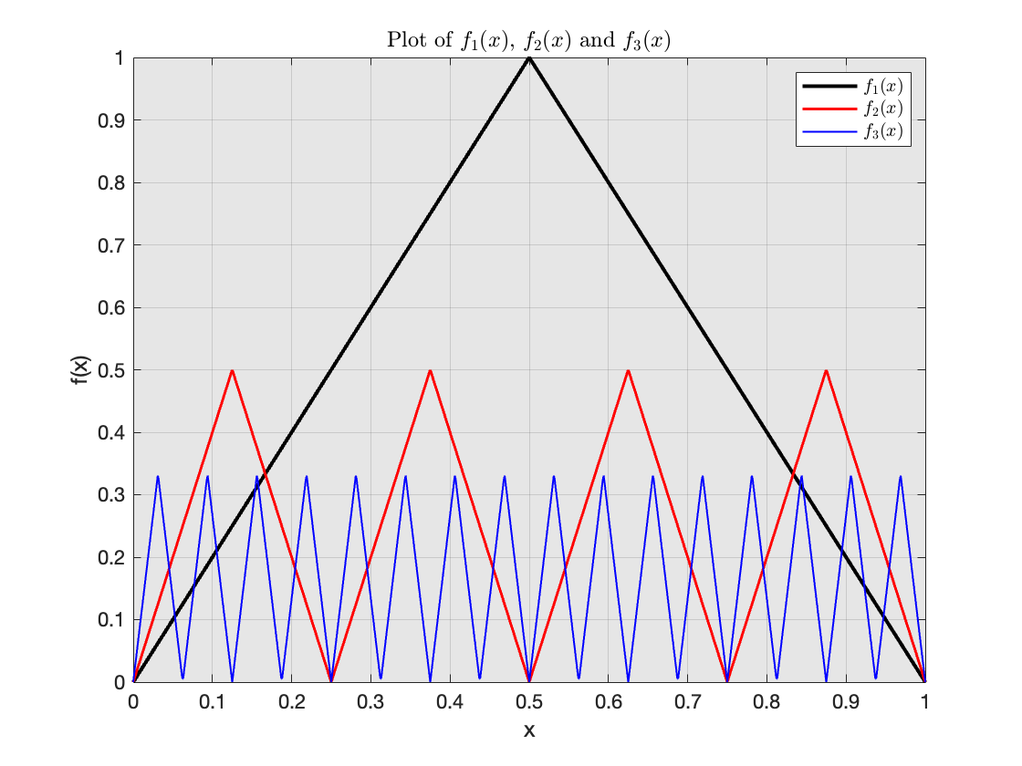
  Figure 7: Plot of function $f_{1}(x),f_{2}(x)$ and $f_{3}(x)$, $f_{4}(x)$ and $f_{5}(x)$ have similar generation processes.

• Example 2: A variant of Weierstrass function. Consider using the strategic Monte Carlo method to optimize a variant of Weierstrass function $f(x)=\sum_{j=1}^{\infty}a^{j}\cos(b^{j}\pi x-1)$ defined on the interval [0, 1]. $f(x)$ is continuous but non-differentiable across its domain. Since the exact function is challenging to graph, we choose $N=100,a=0.75,b=9$, and generate an approximate graph with a horizontal axis interval of $0.002$.

  An optimal random strategy to optimize the global maximum of $f(x)$ can be expressed as $\bm{\theta}^{*}=(\bm{\vartheta}_{1}^{*},\bm{\vartheta}_{2}^{*},\bm{\vartheta}_{3}^{*},\ldots)$, where $\bm{\vartheta}_{i}^{*}$ satisfies:

  $$\bm{\vartheta}_{i}^{*}=\left\{\begin{aligned} 0,\text{ with probability 0.75}\\ 1,\text{ with probability 0.25}\end{aligned}\right.$$

  Then we have $E[\bm{Z}_{i}^{\bm{\theta}^{*}}]=E\left[Y_{1,i}I\{\bm{\vartheta}_{i}^{*}=0\}+X_{1,i}I\{\bm{\vartheta}_{i}^{*}=1\}\right]=0.25$. According to the law of large numbers, we have:

  $$\frac{S_{n}^{\bm{\theta}^{*}}}{n}\rightarrow 0.25,\quad P\text{-a.s., as }n\rightarrow\infty.$$

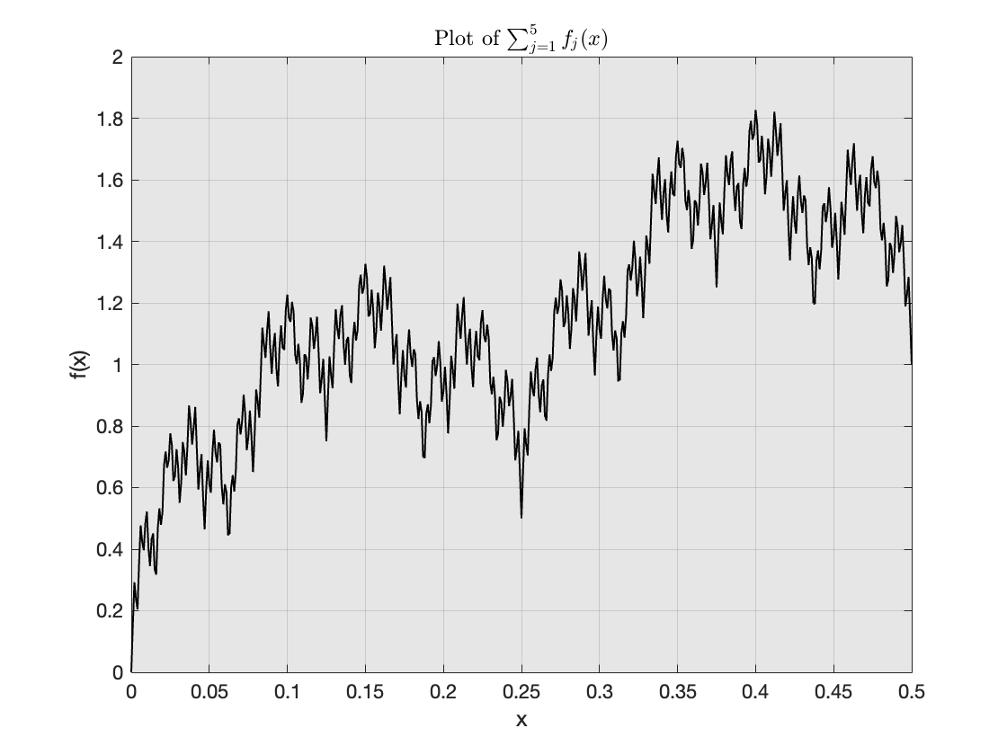
(a)

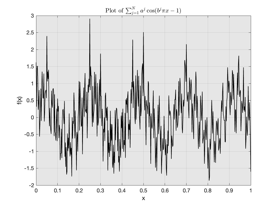
(b)

Figure 8: Two examples of using strategic Monte Carlo method to optimize non-differentiable functions.

Proofs

In this section, we give the proof of the main theorems in Section 2. The Theorem 2.1 can be viewed as a corollary of a general nonlinear limit theorem of Chen, Epstein, and Zhang (2024); we omit its proof here.

Firstly, we present the proof of the strategic law of large numbers (Theorem 2.2). The following lemma can be regarded as a weak form of strategic law for large numbers.

Lemma 5.1.

Let $\varphi\in C_{b}^{3}(\mathbb{R}^{d})$, the space of bounded and three-times continuously differentiable functions with bounded derivatives of all orders less than or equal to three, satisfy the assumptions (A.1) and (A.2) in Theorem 2.2 with $f$ replaced by $\varphi$.

Furthermore, we assume that there exists a constant $L>0$ such that for any $j=1,\cdots,d$, $|X_{j}|<L$ and $|Y_{j}|<L$. Let $N>0$ be the smallest $n$ such that

$$\frac{2L}{n+1}<\min_{1\leq i\leq d}\min_{1\leq j\leq c_{i}^{k_{i}}}\{b_{i}^{j}-c_{i}^{j},c_{i}^{j}-b_{i}^{j-1}\}$$

Consider the strategy $\bm{\theta}^{c}=(\bm{\vartheta}^{c}_{1},\cdots,\bm{\vartheta}_{m}^{c},\cdots)$, where $\bm{\vartheta}_{m}^{c}=(\vartheta^{c}_{m1},\cdots,\vartheta_{md}^{c})$ is defined by

$$\vartheta_{mi}^{c}=\left\{\begin{array}[]{rl}1,&\text{if }\partial_{x_{i}}\varphi\left(\frac{S_{m-1}^{\bm{\theta}^{c}}}{m-1}\right)\geq 0;\\ 0,&\text{otherwise},\end{array}\right.\quad i=1,\cdots,d.$$ [5.1]

Then we have

$$\liminf_{n\to\infty}\left\{E\left[\varphi\left(\frac{S_{n}^{\bm{\theta}^{c}}}{n}\right)\right]-E\left[\sum_{j_{1}=1}^{K_{1}}\cdots\sum_{j_{d}=1}^{K_{d}}\varphi\left(c_{1}^{j_{1}},c_{2}^{j_{2}},\cdots,c_{d}^{j_{d}}\right)I\left\{\frac{S_{N}^{\bm{\theta}^{c}}}{N}\in\Gamma(j_{1},\cdots,j_{d})\right\}\right]\right\}\geq 0,$$ [5.2]

where $\Gamma(j_{1},\cdots,j_{d})=(b_{1}^{j_{1}-1},b_{1}^{j_{1}}]\times\cdots\times(b_{d}^{j_{d}-1},b_{d}^{j_{d}}].$

Proof: For convenience, we only give the proof for the case $d=2$, it can be proved similarly for the general case.

For any large enough $n>N$, it can be checked that

$$E\left[\varphi\left(\frac{S_{n}^{\bm{\theta}^{c}}}{n}\right)\right]-E\left[\sum_{j_{1}=1}^{K_{1}}\sum_{j_{2}=1}^{K_{2}}\varphi\left(c_{1}^{j_{1}},c_{2}^{j_{2}}\right)I\left\{\frac{S_{N}^{\bm{\theta}^{c}}}{N}\in\Gamma(j_{1},j_{2})\right\}\right]$$

$$= \sum_{m=1}^{n}\sum_{j_{1}=1}^{K_{1}}\sum_{j_{2}=1}^{K_{2}}E\left[\left[\varphi\left(\frac{S_{m}^{\bm{\theta}^{c}}}{n}+\frac{n-m}{n}\left(c_{1}^{j_{1}},c_{2}^{j_{2}}\right)\right)\right.\right.$$

$$\hskip 85.35826pt\left.\left.-\varphi\left(\frac{S_{m-1}^{\bm{\theta}^{c}}}{n}+\frac{n-m+1}{n}\left(c_{1}^{j_{1}},c_{2}^{j_{2}}\right)\right)\right]I\left\{\frac{S_{N}^{\bm{\theta}^{c}}}{N}\in\Gamma(j_{1},j_{2})\right\}\right]$$

$$=: \sum_{m=1}^{n}\sum_{j_{1}=1}^{K_{1}}\sum_{j_{2}=1}^{K_{2}}E\left[D_{x}\,\varphi\left(\frac{S_{m-1}^{\bm{\theta}^{c}}}{n}+\frac{n-m+1}{n}\left(c_{1}^{j_{1}},c_{2}^{j_{2}}\right)\right)\cdot\frac{\bm{Z}_{m}^{\bm{\theta}^{c}}-\left(c_{1}^{j_{1}},c_{2}^{j_{2}}\right)}{n}I\left\{\frac{S_{N}^{\bm{\theta}^{c}}}{N}\in\Gamma(j_{1},j_{2})\right\}\right]+R_{n}$$

where $D_{x}\varphi=(\partial_{x_{1}}\varphi,\partial_{x_{2}}\varphi)$ denotes the gradient vector of $\varphi$. It follows from Taylor’s expansion that for any $x,y\in\mathbb{R}^{d}$,

$$\left|\varphi(x+y)-\varphi(x)-D_{x}\,\varphi(x)\cdot y\right|\leq C\|y\|^{2},$$ [5.3]

where $C$ is a constant depend only on the bound of the second derivatives of $\varphi$. For any $1\leq m\leq n,$ taking $x=\frac{S_{m-1}^{\bm{\theta}^{c}}}{n}+\frac{n-m+1}{n}\left(c_{1}^{j_{1}},c_{2}^{j_{2}}\right),y=\frac{\bm{Z}_{m}^{\bm{\theta}^{c}}-\left(c_{1}^{j_{1}},c_{2}^{j_{2}}\right)}{n}$ in [5.3], we obtain

$$|R_{n}|\leq \frac{C}{n^{2}}\sum_{m=1}^{n}\sum_{j_{1}=1}^{K_{1}}\sum_{j_{2}=1}^{K_{2}}E[\|\bm{Z}_{m}^{\bm{\theta}^{c}}\|^{2}+\|\left(c_{1}^{j_{1}},c_{2}^{j_{2}}\right)\|^{2}]\to 0,\text{ as }n\to\infty.$$

On the other hand, for any $N<m\leq n$, if $\frac{S_{N}^{\bm{\theta}^{c}}}{N}\in\Gamma(j_{1},j_{2})$, then one have $\frac{S_{m}^{\bm{\theta}^{c}}}{m}\in\Gamma(j_{1},j_{2})$. Set $\lambda_{n}^{m}=\frac{m-1}{n}$, then

$$E\left[D_{x}\,\varphi\left(\tfrac{S_{m-1}^{\bm{\theta}^{c}}}{n}+\tfrac{n-m+1}{n}\left(c_{1}^{j_{1}},c_{2}^{j_{2}}\right)\right)\cdot\tfrac{\bm{Z}_{m}^{\bm{\theta}^{c}}-\left(c_{1}^{j_{1}},c_{2}^{j_{2}}\right)}{n}I\left\{\tfrac{S_{N}^{\bm{\theta}^{c}}}{N}\in\Gamma(j_{1},j_{2})\right\}\right]$$

$$= \sum_{i=1}^{2}E\left[\partial_{x_{i}}\varphi\left(\tfrac{S_{m-1}^{\bm{\theta}^{c}}}{n}+\tfrac{n-m+1}{n}\left(c_{1}^{j_{1}},c_{2}^{j_{2}}\right)\right)\tfrac{Z_{mi}^{\bm{\theta}^{c}}-c_{i}^{j_{i}}}{n}I\left\{\tfrac{S_{N}^{\bm{\theta}^{c}}}{N}\in\Gamma(j_{1},j_{2})\right\}\right]$$

$$= \sum_{i=1}^{2}E\left[\partial_{x_{i}}\varphi\left(\lambda_{n}^{m}\tfrac{S_{m-1}^{\bm{\theta}^{c}}}{m-1}+(1-\lambda_{n}^{m})\left(c_{1}^{j_{1}},c_{2}^{j_{2}}\right)\right)\tfrac{X_{m,i}-c_{i}^{j_{i}}}{n}I\left\{\partial_{x_{i}}\varphi\left(\tfrac{S_{m-1}^{\bm{\theta}^{c}}}{m-1}\right)\geq 0\right\}I\left\{\tfrac{S_{N}^{\bm{\theta}^{c}}}{N}\in\Gamma(j_{1},j_{2})\right\}\right]$$

$$+\sum_{i=1}^{2}E\left[\partial_{x_{i}}\varphi\left(\lambda_{n}^{m}\tfrac{S_{m-1}^{\bm{\theta}^{c}}}{m-1}+(1-\lambda_{n}^{m})\left(c_{1}^{j_{1}},c_{2}^{j_{2}}\right)\right)\tfrac{Y_{m,i}-c_{i}^{j_{i}}}{n}I\left\{\partial_{x_{i}}\varphi\left(\tfrac{S_{m-1}^{\bm{\theta}^{c}}}{m-1}\right)<0\right\}I\left\{\tfrac{S_{N}^{\bm{\theta}^{c}}}{N}\in\Gamma(j_{1},j_{2})\right\}\right]$$

$$= \sum_{i=1}^{2}E\left[\partial_{x_{i}}\varphi\left(\lambda_{n}^{m}\tfrac{S_{m-1}^{\bm{\theta}^{c}}}{m-1}+(1-\lambda_{n}^{m})\left(c_{1}^{j_{1}},c_{2}^{j_{2}}\right)\right)\tfrac{\overline{\mu}_{i}-c_{i}^{j_{i}}}{n}I\left\{\partial_{x_{i}}\varphi\left(\tfrac{S_{m-1}^{\bm{\theta}^{c}}}{m-1}\right)\geq 0\right\}I\left\{\tfrac{S_{N}^{\bm{\theta}^{c}}}{N}\in\Gamma(j_{1},j_{2})\right\}\right]$$

$$+\sum_{i=1}^{2}E\left[\partial_{x_{i}}\varphi\left(\lambda_{n}^{m}\tfrac{S_{m-1}^{\bm{\theta}^{c}}}{m-1}+(1-\lambda_{n}^{m})\left(c_{1}^{j_{1}},c_{2}^{j_{2}}\right)\right)\tfrac{\underline{\mu}_{i}-c_{i}^{j_{i}}}{n}I\left\{\partial_{x_{i}}\varphi\left(\tfrac{S_{m-1}^{\bm{\theta}^{c}}}{m-1}\right)<0\right\}I\left\{\tfrac{S_{N}^{\bm{\theta}^{c}}}{N}\in\Gamma(j_{1},j_{2})\right\}\right].$$

Since

$$\left\{\partial_{x_{i}}\varphi\left(x\right)\geq 0,x\in\Gamma(j_{1},j_{2})\right\}=\left\{x=(x_{1},x_{2})\in\Gamma(j_{1},j_{2}):x_{i}\leq c_{i}^{j_{i}}\right\}=:M_{i}^{j_{i}}$$

Then for any $y\in M_{i}^{j_{i}}$ and any $\lambda\in(0,1)$, we have $\lambda y+(1-\lambda)\left(c_{1}^{j_{1}},c_{2}^{j_{2}}\right)\in M_{i}^{j_{i}}$. Therefore we have, for any $j=1,2$,

$$\partial_{x_{i}}\varphi\left(\lambda_{n}^{m}\frac{S_{m-1}^{\bm{\theta}^{c}}}{m-1}+(1-\lambda_{n}^{m})\left(c_{1}^{j_{1}},c_{2}^{j_{2}}\right)\right)I\left\{\partial_{x_{i}}\varphi\left(\tfrac{S_{m-1}^{\bm{\theta}^{c}}}{m-1}\right)\geq 0\right\}I\left\{\tfrac{S_{N}^{\bm{\theta}^{c}}}{N}\in\Gamma(j_{1},j_{2})\right\}\geq 0$$

and similarly,

$$\partial_{x_{i}}\varphi\left(\lambda_{n}^{m}\frac{S_{m-1}^{\bm{\theta}^{c}}}{m-1}+(1-\lambda_{n}^{m})\left(c_{1}^{j_{1}},c_{2}^{j_{2}}\right)\right)I\left\{\partial_{x_{i}}\varphi\left(\tfrac{S_{m-1}^{\bm{\theta}^{c}}}{m-1}\right)<0\right\}I\left\{\tfrac{S_{N}^{\bm{\theta}^{c}}}{N}\in\Gamma(j_{1},j_{2})\right\}\leq 0.$$

And these will lead to, for $N<m\leq n$,

$$E\left[D_{x}\,\varphi\left(\frac{S_{m-1}^{\bm{\theta}^{c}}}{n}+\frac{n-m+1}{n}\left(c_{1}^{j_{1}},c_{2}^{j_{2}}\right)\right)\cdot\frac{\bm{Z}_{m}^{\bm{\theta}^{c}}-\left(c_{1}^{j_{1}},c_{2}^{j_{2}}\right)}{n}I\left\{\tfrac{S_{N}^{\bm{\theta}^{c}}}{N}\in\Gamma(j_{1},j_{2})\right\}\right]\geq 0.$$

That is,

$$\liminf_{n\to\infty}\left\{E\left[\varphi\left(\tfrac{S_{n}^{\bm{\theta}^{c}}}{n}\right)\right]-E\left[\sum_{j_{1}=1}^{K_{1}}\sum_{j_{2}=1}^{K_{2}}\varphi\left(c_{1}^{j_{1}},c_{2}^{j_{2}}\right)I\left\{\tfrac{S_{N}^{\bm{\theta}^{c}}}{N}\in\Gamma(j_{1},j_{2})\right\}\right]\right\}$$

$$\geq \liminf_{n\to\infty}\sum_{m=1}^{n}\sum_{j_{1}=1}^{K_{1}}\sum_{j_{2}=1}^{K_{2}}E\left[D_{x}\,\varphi\left(\tfrac{S_{m-1}^{\bm{\theta}^{c}}}{n}+\tfrac{n-m+1}{n}\left(c_{1}^{j_{1}},c_{2}^{j_{2}}\right)\right)\cdot\tfrac{\bm{Z}_{m}^{\bm{\theta}^{c}}-\left(c_{1}^{j_{1}},c_{2}^{j_{2}}\right)}{n}I\left\{\tfrac{S_{N}^{\bm{\theta}^{c}}}{N}\in\Gamma(j_{1},j_{2})\right\}\right]$$

$$-\lim_{n\to\infty}|R_{n}|$$

$$\geq \liminf_{n\to\infty}\sum_{m=1}^{N}\sum_{j_{1}=1}^{K_{1}}\sum_{j_{2}=1}^{K_{2}}E\left[D_{x}\,\varphi\left(\tfrac{S_{m-1}^{\bm{\theta}^{c}}}{n}+\tfrac{n-m+1}{n}\left(c_{1}^{j_{1}},c_{2}^{j_{2}}\right)\right)\cdot\tfrac{\bm{Z}_{m}^{\bm{\theta}^{c}}-\left(c_{1}^{j_{1}},c_{2}^{j_{2}}\right)}{n}I\left\{\tfrac{S_{N}^{\bm{\theta}^{c}}}{N}\in\Gamma(j_{1},j_{2})\right\}\right]$$

$$+\liminf_{n\to\infty}\sum_{m=N+1}^{n}\sum_{j_{1}=1}^{K_{1}}\sum_{j_{2}=1}^{K_{2}}E\left[D_{x}\,\varphi\left(\tfrac{S_{m-1}^{\bm{\theta}^{c}}}{n}+\tfrac{n-m+1}{n}\left(c_{1}^{j_{1}},c_{2}^{j_{2}}\right)\right)\cdot\tfrac{\bm{Z}_{m}^{\bm{\theta}^{c}}-\left(c_{1}^{j_{1}},c_{2}^{j_{2}}\right)}{n}I\left\{\tfrac{S_{N}^{\bm{\theta}^{c}}}{N}\in\Gamma(j_{1},j_{2})\right\}\right]$$

$$-\lim_{n\to\infty}|R_{n}|$$

$$\geq 0.$$

The proof of Step 2 is completed. $\blacksquare$

Next we give the proof of Theorem 2.2.

Proof of Theorem 2.2: Firstly we prove that, for any $\varepsilon>0$,

$$\lim_{n\to\infty}P\left(\frac{S_{n}^{\bm{\theta}^{*}}}{n}\in\mathcal{M}_{\varepsilon}\right)=1,$$

where

$$\mathcal{M}_{\varepsilon}=\bigcup_{j_{1}=1}^{K_{1}}\cdots\bigcup_{j_{d}=1}^{K_{d}}\left\{(c_{1}^{j_{1}},\cdots,c_{d}^{j_{d}})-\bm{\varepsilon}\leq x\leq(c_{1}^{j_{1}},\cdots,c_{d}^{j_{d}})+\bm{\varepsilon}\right\}$$

and $\bm{\varepsilon}=(\varepsilon,\cdots,\varepsilon)$ is a $d$-dimensional vector. Let $\psi\in C_{b}^{3}(\mathbb{R}^{d})$ satisfy the assumption (A.1) and (A.2). Furthermore suppose that for $x\notin\mathcal{M}_{\varepsilon}$, $\psi(x)\leq 0$, for $x\in\mathcal{M}_{\varepsilon}$, $0\leq\psi(x)\leq 1$ and $\psi(c_{1}^{j_{1}},\cdots,c_{d}^{j_{d}})=1$. Then the strategy $\bm{\theta}^{*}$ [2.11] is same as the strategy $\bm{\theta}^{c}$, which is defined by [5.1] via $\psi$, and we have

$$\lim_{n\to\infty}P\left(\frac{S_{n}^{\bm{\theta}^{*}}}{n}\in\mathcal{M}_{\varepsilon}\right)$$

$$= \lim_{n\to\infty}E\left[I{\left\{\frac{S_{n}^{\bm{\theta}^{*}}}{n}\in\mathcal{M}_{\varepsilon}\right\}}\right]$$

$$\geq \lim_{n\to\infty}E\left[\psi\left(\frac{S_{n}^{\bm{\theta}^{*}}}{n}\right)\right]-1+1$$

$$= \liminf_{n\to\infty}\left\{E\left[\psi\left(\frac{S_{n}^{\bm{\theta}^{*}}}{n}\right)\right]-E\left[\sum_{j_{1}=1}^{K_{1}}\cdots\sum_{j_{d}=1}^{K_{d}}\psi\left(c_{1}^{j_{1}},c_{2}^{j_{2}},\cdots,c_{d}^{j_{d}}\right)I\left\{\frac{S_{N}^{\bm{\theta}^{*}}}{N}\in\Gamma(j_{1},\cdots,j_{d})\right\}\right]\right\}+1$$

$$\geq 1$$

where the last inequality is due to Lemma 5.1. Then we have $S_{n}^{\bm{\theta}^{*}}/n$ converge to one point of $\mathcal{M}$ in probability.

On the other hand, since we suppose that $(\Omega,\mathcal{F},P)$ is a discrete probability space, then we have convergence in probability and convergence almost surely are equivalent. That is, we have [2.12]. $\blacksquare$

Secondly, we give the proof of the convergence rate.

Proof of Theorem 2.3: For any $\bm{\theta}\in\Theta$, set $\tilde{S}_{n}^{\bm{\theta}}=\sum_{i=1}^{n}E\left[\bm{Z}_{i}^{\bm{\theta}}|\mathcal{H}_{i-1}^{\bm{\theta}}\right]$, then we have $\frac{\tilde{S}_{n}^{\bm{\theta}}}{n}\in\Gamma$, $P$-a.s., which implies that

$$E\left[f\left(\frac{S_{n}^{\bm{\theta}^{*}}}{n}\right)\right]-\sup_{x\in\Gamma}f(x)\leq E\left[f\left(\frac{S_{n}^{\bm{\theta}^{*}}}{n}\right)-f\left(\frac{\tilde{S}_{n}^{\bm{\theta}^{*}}}{n}\right)\right]\leq\frac{L_{f}}{n}\left(E\left[\|S_{n}^{\bm{\theta}^{*}}-\tilde{S}_{n}^{\bm{\theta}^{*}}\|^{2}\right]\right)^{\frac{1}{2}}.$$

It can be checked that,

$$E\left[\|S_{n}^{\bm{\theta}^{*}}-\tilde{S}_{n}^{\bm{\theta}^{*}}\|^{2}\right]= \sum_{j=1}^{d}\sum_{i=1}^{n}E\left[(Z_{ij}^{\bm{\theta}^{*}}-E[Z_{ij}^{\bm{\theta}^{*}}|\mathcal{H}_{i-1}^{\bm{\theta}^{*}}])^{2}\right]$$

$$\leq \sum_{j=1}^{d}\sum_{i=1}^{n}\max\{Var(X_{j}),Var({Y_{j}})\}=nd\sigma^{2}.$$

Therefore, we have

$$E\left[f\left(\frac{S_{n}^{\bm{\theta}^{*}}}{n}\right)\right]-f(x^{*})\leq\frac{L_{f}\sigma\sqrt{d}}{\sqrt{n}}.$$

On the other hand,

$$E\left[f\left(\frac{S_{n}^{\bm{\theta}^{*}}}{n}\right)\right]-f(x^{*})$$

$$= \sum_{m=1}^{n}E\left[f\left(\frac{S_{m}^{\bm{\theta}^{*}}}{n}+\frac{(n-m)x^{*}}{n}\right)-f\left(\frac{S_{m-1}^{\bm{\theta}^{*}}}{n}+\frac{(n-m+1)x^{*}}{n}\right)\right]$$

$$\geq \sum_{m=1}^{n}E\left[\frac{Z_{m}^{\bm{\theta}^{*}}-x^{*}}{n}\cdot D_{x}f\left(\frac{S_{m-1}^{\bm{\theta}^{*}}}{n}+\frac{(n-m+1)x^{*}}{n}\right)\right]-\frac{K_{f}}{n^{2}}\sum_{m=1}^{n}E\left[\left\|Z_{m}^{\bm{\theta}^{*}}-x^{*}\right\|^{2}\right]$$

$$\geq -\frac{K_{f}\left[d\sigma^{2}+\sum_{j=1}^{d}(\overline{\mu}_{j}-\underline{\mu}_{j})^{2}\right]}{n}.$$

The last inequality is due to, for any $1\leq m\leq n$, set $\lambda_{n}^{m}=\frac{m-1}{n}$, we have

$$E\left[D_{x}\,f\left(\frac{S_{m-1}^{\bm{\theta}^{*}}}{n}+\frac{n-m+1}{n}x^{*}\right)\cdot\frac{\bm{Z}_{m}^{\bm{\theta}^{*}}-x^{*}}{n}\right]$$

$$= \sum_{j=1}^{d}E\left[\partial_{x_{j}}f\left(\frac{S_{m-1}^{\bm{\theta}^{*}}}{n}+\frac{n-m+1}{n}x^{*}\right)\frac{Z_{mj}^{\bm{\theta}^{*}}-x^{*}_{j}}{n}\right]$$

$$= \sum_{j=1}^{d}E\left[\partial_{x_{j}}f\left(\lambda_{n}^{m}\frac{S_{m-1}^{\bm{\theta}^{*}}}{m-1}+(1-\lambda_{n}^{m})x^{*}\right)\frac{X_{m,j}-x^{*}_{j}}{n}I\left\{\partial_{x_{j}}f\left(\tfrac{S_{m-1}^{\bm{\theta}^{*}}}{m-1}\right)\geq 0\right\}\right]$$

$$+\sum_{j=1}^{d}E\left[\partial_{x_{j}}f\left(\lambda_{n}^{m}\frac{S_{m-1}^{\bm{\theta}^{*}}}{m-1}+(1-\lambda_{n}^{m})x^{*}\right)\frac{Y_{m,j}-x^{*}_{j}}{n}I\left\{\partial_{x_{j}}f\left(\tfrac{S_{m-1}^{\bm{\theta}^{*}}}{m-1}\right)<0\right\}\right]$$

$$= \sum_{j=1}^{d}E\left[\partial_{x_{j}}f\left(\lambda_{n}^{m}\frac{S_{m-1}^{\bm{\theta}^{*}}}{m-1}+(1-\lambda_{n}^{m})x^{*}\right)\frac{\overline{\mu}_{j}-x^{*}_{j}}{n}I\left\{\partial_{x_{j}}f\left(\tfrac{S_{m-1}^{\bm{\theta}^{*}}}{m-1}\right)\geq 0\right\}\right]$$

$$+\sum_{j=1}^{d}E\left[\partial_{x_{j}}f\left(\lambda_{n}^{m}\frac{S_{m-1}^{\bm{\theta}^{*}}}{m-1}+(1-\lambda_{n}^{m})x^{*}\right)\frac{\underline{\mu}_{j}-x^{*}_{j}}{n}I\left\{\partial_{x_{j}}f\left(\tfrac{S_{m-1}^{\bm{\theta}^{*}}}{m-1}\right)<0\right\}\right].$$

Since

$$\left\{\partial_{x_{j}}f\left(x\right)\geq 0\right\}=\left\{x=(x_{1},\cdots,x_{d})\in\Gamma_{\delta}:x_{j}\leq x^{*}_{j}\right\}=:M_{j}$$

Then for any $y\in M_{j}$ and any $\lambda\in(0,1)$, we have $\lambda y+(1-\lambda)x^{*}\in M_{j}$. Therefore we have, for any $j=1,\cdots,d$,

$$\partial_{x_{j}}f\left(\lambda_{n}^{m}\frac{S_{m-1}^{\bm{\theta}^{*}}}{m-1}+(1-\lambda_{n}^{m})x^{*}\right)I\left\{\partial_{x_{j}}f\left(\tfrac{S_{m-1}^{\bm{\theta}^{*}}}{m-1}\right)\geq 0\right\}\geq 0$$

and similarly,

$$\partial_{x_{j}}f\left(\lambda_{n}^{m}\frac{S_{m-1}^{\bm{\theta}^{*}}}{m-1}+(1-\lambda_{n}^{m})x^{*}\right)I\left\{\partial_{x_{j}}f\left(\tfrac{S_{m-1}^{\bm{\theta}^{*}}}{m-1}\right)<0\right\}\leq 0.$$

And these will lead to

$$E\left[D_{x}\,f\left(\frac{S_{m-1}^{\bm{\theta}^{*}}}{n}+\frac{n-m+1}{n}x^{*}\right)\cdot\frac{\bm{Z}_{m}^{\bm{\theta}^{*}}-x^{*}}{n}\right]\geq 0.$$

Therefore, we have

$$\left|E\left[f\left(\frac{S_{n}^{\bm{\theta}^{*}}}{n}\right)\right]-f(x^{*})\right|\leq\max\left\{\frac{L_{f}\sigma\sqrt{d}}{\sqrt{n}},\frac{K_{f}\left(d\sigma^{2}+\sum_{j=1}^{d}(\overline{\mu}_{j}-\underline{\mu}_{j})^{2}\right)}{n}\right\}$$

For any $x\in\mathbb{R}^{d}$, define $\phi(x)=\|x-x^{*}\|^{2}$, therefore we have $\phi(x^{*})=0$ and by Taylor’s formula

$$E\left[\left\|\frac{S_{n}^{\bm{\theta}^{*}}}{n}-x^{*}\right\|^{2}\right]= E\left[\phi\left(\frac{S_{n}^{\bm{\theta}^{*}}}{n}\right)\right]-\phi(x^{*})$$

$$= \sum_{m=1}^{n}E\left[\phi\left(\frac{S_{m}^{\bm{\theta}^{*}}}{n}+\frac{n-m}{n}x^{*}\right)-\phi\left(\frac{S_{m-1}^{\bm{\theta}^{*}}}{n}+\frac{n-m+1}{n}x^{*}\right)\right]$$

$$= \sum_{m=1}^{n}E\left[\frac{Z_{m}^{\bm{\theta}^{*}}-x^{*}}{n}\cdot D_{x}\phi\left(\frac{S_{m-1}^{\bm{\theta}^{*}}}{n}+\frac{(n-m+1)x^{*}}{n}\right)\right]+\frac{1}{n^{2}}\sum_{m=1}^{n}E\left[\left\|Z_{m}^{\bm{\theta}^{*}}-x^{*}\right\|^{2}\right]$$

It can be checked that,

$$E\left[D_{x}\,\phi\left(\frac{S_{m-1}^{\bm{\theta}^{*}}}{n}+\frac{n-m+1}{n}x^{*}\right)\cdot\frac{\bm{Z}_{m}^{\bm{\theta}^{*}}-x^{*}}{n}\right]$$

$$= \sum_{j=1}^{d}E\left[\partial_{x_{j}}\phi\left(\frac{S_{m-1}^{\bm{\theta}^{*}}}{n}+\frac{n-m+1}{n}x^{*}\right)\frac{Z_{mj}^{\bm{\theta}^{*}}-x^{*}_{j}}{n}\right]$$

$$= \sum_{j=1}^{d}E\left[2\left(\frac{\sum_{i=1}^{m-1}Z_{ij}^{\bm{\theta}^{*}}}{n}-\frac{m-1}{n}x^{*}_{j}\right)\frac{Z_{mj}^{\bm{\theta}^{*}}-x^{*}_{j}}{n}\right]$$

$$= \sum_{j=1}^{d}E\left[2\left(\frac{\sum_{i=1}^{m-1}Z_{ij}^{\bm{\theta}^{*}}}{n}-\frac{m-1}{n}x^{*}_{j}\right)\frac{X_{m,j}-x^{*}_{j}}{n}I\left\{\partial_{x_{j}}f\left(\tfrac{S_{m-1}^{\bm{\theta}^{*}}}{m-1}\right)\geq 0\right\}\right]$$

$$+\sum_{j=1}^{d}E\left[2\left(\frac{\sum_{i=1}^{m-1}Z_{ij}^{\bm{\theta}^{*}}}{n}-\frac{m-1}{n}x^{*}_{j}\right)\frac{Y_{m,j}-x^{*}_{j}}{n}I\left\{\partial_{x_{j}}f\left(\tfrac{S_{m-1}^{\bm{\theta}^{*}}}{m-1}\right)<0\right\}\right]$$

$$= \sum_{j=1}^{d}E\left[\frac{2(m-1)}{n}\left(\frac{\sum_{i=1}^{m-1}Z_{ij}^{\bm{\theta}^{*}}}{m-1}-x^{*}_{j}\right)\frac{\overline{\mu}_{j}-x^{*}_{j}}{n}I\left\{\partial_{x_{j}}f\left(\tfrac{S_{m-1}^{\bm{\theta}^{*}}}{m-1}\right)\geq 0\right\}\right]$$

$$+\sum_{j=1}^{d}E\left[\frac{2(m-1)}{n}\left(\frac{\sum_{i=1}^{m-1}Z_{ij}^{\bm{\theta}^{*}}}{m-1}-x^{*}_{j}\right)\frac{\underline{\mu}_{j}-x^{*}_{j}}{n}I\left\{\partial_{x_{j}}f\left(\tfrac{S_{m-1}^{\bm{\theta}^{*}}}{m-1}\right)<0\right\}\right]$$

Since $\underline{\mu}_{j}\leq x_{j}^{*}\leq\overline{\mu}_{j}$ and

$$\left\{\partial_{x_{j}}f\left(x\right)\geq 0\right\}=\left\{x=(x_{1},\cdots,x_{d})\in\Gamma_{\delta}:x_{j}\leq x^{*}_{j}\right\},$$

we have

$$E\left[D_{x}\,\phi\left(\frac{S_{m-1}^{\bm{\theta}^{*}}}{n}+\frac{n-m+1}{n}x^{*}\right)\cdot\frac{\bm{Z}_{m}^{\bm{\theta}^{*}}-x^{*}}{n}\right]\leq 0,$$

and then

$$E\left[\left\|\frac{S_{n}^{\bm{\theta}^{*}}}{n}-x^{*}\right\|^{2}\right]= \sum_{m=1}^{n}E\left[\frac{Z_{m}^{\bm{\theta}^{*}}-x^{*}}{n}\cdot D_{x}\phi\left(\frac{S_{m-1}^{\bm{\theta}^{*}}}{n}+\frac{(n-m+1)x^{*}}{n}\right)\right]+\frac{1}{n^{2}}\sum_{m=1}^{n}E\left[\left\|Z_{m}^{\bm{\theta}^{*}}-x^{*}\right\|^{2}\right]$$

$$\leq \frac{d\sigma^{2}+\sum_{j=1}^{d}(\overline{\mu}_{j}-\underline{\mu}_{j})^{2}}{n}$$

$\blacksquare$

Thirdly, we present the proof of the convergence with tree search.

Proof of Theorem 2.4: The proof can be structured into tree steps.

Step I. We first prove that every node in a Monte Carlo tree will be searched. The proof is given only for one-dimensional function, for the high dimensional functions can be obtained in a similar way. Without loss of generality, assume that $f(x)$ has $k$ maximum points $\{m_{1},\ldots,m_{k}\}$ (If there exists an interval where all the points are maximum points, then take any one of them). Suppose there is a $\mathcal{L}$-layer Monte Carlo tree, and the value of a node is defined in [2.15]. Let $\Delta_{i}=\max\{f(m_{1}),\ldots,f(m_{k})\}-f(m_{i})$ and $\Delta=\max\{f(m_{1}),\ldots,f(m_{k})\}\}-\min\{f(m_{1}),\ldots,f(m_{k})\}\}$. Following proof shows that any node in the Monte Carlo tree will be searched given a sufficiently large number of explorations. Suppose $s$ is a parent node, and $v_{1}$ and $v_{2}$ are child nodes, then $N(v_{i})\geq{C^{2}}/{(\Delta+C)^{2}}\log N(s),i=1,2$, and $C$ denotes exploration weight. Otherwise, if there exists a child node with several explorations less than ${C^{2}}/{(\Delta+C)^{2}}\log N(s)$, without loss of generality, suppose it is node $v_{1}$, then we have:

$$Q(v_{1})+C\sqrt{\frac{\log N(s)}{N(v_{1})}} >Q(v_{1})+\Delta+C$$

$$\Rightarrow Q(v_{1})+C\sqrt{\frac{\log N(s)}{N(v_{1})}} >Q(v_{2})+C$$

$$\Rightarrow Q(v_{1})+C\sqrt{\frac{\log N(s)}{N(v_{1})}} >Q(v_{2})+C\sqrt{\frac{\log N(s)}{N(v_{2})}},$$

which means that node $v_{1}$ will be searched next time until $N(v_{1})$ exceeds ${C^{2}}/{(\Delta+C)^{2}}\log N(s)$. Thus we complete the proof that any node in the Monte Carlo tree will be searched given a sufficiently large number of explorations.

Step II. Suppose $x^{*}$ is one of global maximum points of $f$. Let $\delta_{0}=\frac{1}{2}\underset{1\leq i\leq d}{\min}\underset{1\leq j\leq K_{i}}{\min}\{c_{i}^{j}-b_{i}^{j-1},b_{i}^{j}-c_{i}^{j}\}$, $\delta=\frac{1}{2\sqrt{d}}\delta_{0}$ and $x$ be any point in $B(x^{*},\delta_{0})$, where $B(x^{*},\delta_{0})=\{x\in\mathbb{R}^{d}:\|x-x^{*}\|<\delta_{0}\}$. By the definition of the arms in [2.3], assume that $\underset{1\leq i\leq d}{\max}\{|X_{i}|,|Y_{i}|\}<L$. According to optimal strategy $\bm{\theta}^{*}$, we have:

$$\left\|\frac{S_{n+1}^{\bm{\theta}^{*}}}{n+1}-\frac{S_{n}^{\bm{\theta}^{*}}}{n}\right\| =\frac{1}{n+1}\left\|S_{n+1}^{\bm{\theta}^{*}}-\frac{(n+1)S_{n}^{\bm{\theta}^{*}}}{n}\right\|$$

$$\leq\frac{1}{n+1}\left(\left\|S_{n+1}^{\bm{\theta}^{*}}-S_{n}^{\bm{\theta}^{*}}\right\|+\left\|\frac{S_{n}^{\bm{\theta}^{*}}}{n}\right\|\right)$$

$$\leq\frac{2\sqrt{d}L}{n+1}.$$

This indicates that for each $n\geq N_{1}=\left\lceil\frac{2\sqrt{d}L}{\delta_{0}}\right\rceil$, it follows $\left\|\frac{S_{n+1}^{\bm{\theta}^{*}}}{n+1}-\frac{S_{n}^{\bm{\theta}^{*}}}{n}\right\|<\delta_{0}$, which means that when $n$ is sufficiently large, $S_{n}^{\bm{\theta}^{*}}/n$ will not jump out of $B(x^{*},\delta_{0})$.

Next consider how to find such an $x\in B(x^{*},\delta_{0})$. Without loss of generality, assuming that $x^{*}$ is a rational point and $x^{*}=(x_{1}^{*},\ldots,x_{d}^{*})$. Thus for each $x_{i}^{*}$, there exists a unique $\lambda_{i}$ such that $x_{i}^{*}=\lambda_{i}\underline{\mu}_{i}+(1-\lambda_{i})\overline{\mu}_{i}$, where $\lambda_{i}={q_{i}}/{p_{i}}$ and $q_{i}$ and $p_{i}$ are mutually prime. Let $N=N_{1}\prod\limits_{i=1}^{d}p_{i}$ and it follows that $x_{i}^{*}=[{N\lambda_{i}\underline{\mu}_{i}+N(1-\lambda_{i})\overline{\mu}_{i}]}/{N}$. Thus if the $d$ two-armed slot machines are pulled $N$ times, and the left arm of the $i$th slot machine is pulled $N\lambda_{i}$ times, and the right arm is pulled $N(1-\lambda_{i})$ times, which means that $x=(x_{1},\ldots,x_{d})$ with $x_{i}=\left(\sum\limits_{j=1}^{N\lambda_{i}}Y_{i,j}+\sum\limits_{j=1}^{N(1-\lambda_{i})}X_{i,j}\right)/{N}$. According to the definition of the arms in [2.3] and $\delta=\frac{1}{2\sqrt{d}}\underset{1\leq i\leq d}{\min}\underset{1\leq j\leq K}{\min}\{c_{i}^{j}-b_{i}^{j-1},b_{i}^{j}-c_{i}^{j}\}$, it can be obtained that $x_{i}\in(x_{i}^{*}-\delta,x_{i}^{*}+\delta)$, which in turn has $x\in B(x^{*},\delta_{0})$.

Therefore, with the conclusion of Step II, a strategy $\bm{\theta}_{N}$ can be constructed and satisfy $S_{N}^{\bm{\theta}_{N}}/N\in B(x^{*},\delta_{0})$. The conclusion of Step I ensures that $\bm{\theta}_{N}$ can be searched as well. By $\bm{\theta}^{\prime}=(\bm{\vartheta}_{1},\ldots,\bm{\vartheta}_{N},\bm{\vartheta}_{N+1}^{*},\ldots)$ and Theorem 2.2, it follows:

$$\frac{S_{n}^{\bm{\theta}^{\prime}}}{n}\rightarrow x^{*},\quad P\text{-a.s.},\text{ as }n\to\infty.$$

which is equivalent to:

$$T_{n}\rightarrow\underset{x\in\Gamma}{\sup}f(x),\quad P\text{-a.s.},\text{ as }n\to\infty.$$

$\blacksquare$

Proof of Subsection 2.2.4

Let $\hat{f}$ be a bounded Lipschitz continuous extension of $f$ defined on $\mathbb{R}^{d}$. For any $\epsilon>0$, define

$$u_{\epsilon}(t,x)=\sup_{a\in\mathcal{A}(t,1+\epsilon)}E\left[\hat{f}\left(x+\int_{t}^{1+\epsilon}a_{s}ds+\int_{t}^{1+\epsilon}\epsilon\bm{I}_{d}dB_{s}\right)\right]$$ [5.4]

where $\bm{I}_{d}$ is a $d$-dimensional identity matrix and $(B_{t})$ is a $d$-dimensional Brownian motion and $\mathcal{F}_{t}$ is the natural filtration generated by $(B_{t})$. Let $\mathcal{A}(t,T)$ denote the set of all $\{\mathcal{F}_{s}\}$-adapted measurable processes valued in $\Gamma$. It can be checked that $u_{\epsilon}$ is the unique solution of the HJB-equation [2.18] (Yong and Zhou (1999, Theorem 5.2, Ch. 4)), and has the following properties.

Lemma 5.2.

For any fixed $\epsilon>0$, the functions $\{u_{\epsilon}(t,x)\}_{t\in[0,1]}$ satisfy the following properties:

(1)

$u_{\epsilon}(t,\cdot)\in C_{b}^{2}(\mathbb{R}^{d})$ and each element of the gradient vector and Hessian matrix of $u_{\epsilon}(t,\cdot)$ are uniformly bounded for all $t\in[0,1]$.

(2)

Dynamic programming principle: For any $\gamma\in[0,1+\epsilon-t]$,

$$u_{\epsilon}(t,x)=\sup_{a\in\mathcal{A}(t,t+\delta)}E\left[u_{\epsilon}\left(t+\gamma,x+\int_{t}^{t+\gamma}a_{s}ds+\int_{t}^{t+\gamma}\epsilon\bm{I}_{d}dB_{s}\right)\right],\;x\in\mathbb{R}^{d}.$$

(3)

There exists a constant $C$, depends only on the uniform bound of $D_{x}^{2}\,u_{\epsilon}(t,\cdot)$, such that

$$\limsup\limits_{n\rightarrow\infty}\sum\limits_{m=1}^{n}\sup\limits_{x\in\mathbb{R}^{d}}\left|u_{\epsilon}(\tfrac{m-1}{n},x)-u_{\epsilon}\left(\tfrac{m}{n},x\right)-\sup_{p\in\Gamma}\left[D_{x}u_{\epsilon}\left(\tfrac{m}{n},x\right)\cdot p\right]\right|\leq C\epsilon^{2}.$$

Proof: Since $u_{\epsilon}$ is the solution of the HJB-equation (5.5) (Yong and Zhou (1999, Theorem 5.2, Ch. 4)).

$$\left\{\begin{array}[]{l}\displaystyle\partial_{t}u_{\epsilon}(t,x)+\sup_{p\in\Gamma}\left[D_{x}u_{\epsilon}(t,x)\cdot p\right]+\frac{\epsilon^{2}}{2}\textrm{tr}\left[D_{x}^{2}u_{\epsilon}(t,x)\right]=0,\quad(t,x)\in[0,1+\epsilon)\times\mathbb{R}^{d}\\ u_{\epsilon}(1+\epsilon,x)=\hat{f}(x).\end{array}\right.$$ [5.5]

By Theorem C.4.5 in Peng (2019), $\exists\beta\in(0,1)$ such that

$$\|u_{\epsilon}\|_{C^{1+\beta/2,2+\beta}([0,1]\times\mathbb{R}^{d})}<\infty.$$

Here $\|\cdot\|_{C^{1+\beta/2,2+\beta}([0,1]\times\mathbb{R}^{d})}$ is the Krylov (1987) norm on $C^{1+\beta/2,2+\beta}([0,1]\times\mathbb{R}^{d})$, the set of (continuous and) suitably differentiable functions on $[0,1]\times\mathbb{R}^{d}$.

This proves (1).

(2) follows directly from the classical dynamic programming principle (Yong and Zhou (1999, Theorem 3.3, Ch. 4)).

Prove (3): By Ito’s formula,

$$\sum\limits_{m=1}^{n}\sup\limits_{x\in\mathbb{R}^{d}}\left|u_{\epsilon}(\tfrac{m-1}{n},x)-u_{\epsilon}\left(\tfrac{m}{n},x\right)-\sup_{p\in\Gamma}\left[D_{x}u_{\epsilon}\left(\tfrac{m}{n},x\right)\cdot p\right]\right|$$

$$= \sum_{m=1}^{n}\sup_{x\in\mathbb{R}^{d}}\left|\sup_{a\in\mathcal{A}(\frac{m-1}{n},\frac{m}{n})}\!\!E\left[u_{\epsilon}\left(\frac{m}{n},x+\int_{\frac{m-1}{n}}^{\frac{m}{n}}a_{s}ds+\int_{\frac{m-1}{n}}^{\frac{m}{n}}\epsilon\bm{I}_{d}dB_{s}\right)\right]-u_{\epsilon}\left(\tfrac{m}{n},x\right)-\sup_{p\in\Gamma}\left[D_{x}u_{\epsilon}\left(\tfrac{m}{n},x\right)\cdot p\right]\right|$$

$$= \sum_{m=1}^{n}\sup_{x\in\mathbb{R}^{d}}\left|\sup_{a\in\mathcal{A}(\frac{m-1}{n},\frac{m}{n})}\!\!E\left[\int_{\frac{m-1}{n}}^{\frac{m}{n}}D_{x}u_{\epsilon}\left(\frac{m}{n},x+\int_{\frac{m-1}{n}}^{s}a_{s}ds+\int_{\frac{m-1}{n}}^{\frac{m}{n}}\epsilon\bm{I}_{d}dB_{s}\right)\cdot a_{s}ds\right.\right.$$

$$\hskip 56.9055pt\left.+\frac{\epsilon^{2}}{2}\int_{\frac{m-1}{n}}^{\frac{m}{n}}\textup{tr}\left[D_{x}^{2}u_{\epsilon}\left(\frac{m}{n},x+\int_{\frac{m-1}{n}}^{s}a_{s}ds+\int_{\frac{m-1}{n}}^{s}\epsilon\bm{I}_{d}dB_{s}\right)\right]ds\right]-\sup_{p\in\Gamma}\left[D_{x}u_{\epsilon}\left(\tfrac{m}{n},x\right)\cdot p\right]\Bigg{|}$$

$$\leq \frac{C}{n}\sum_{m=1}^{n}\left|\sup_{a\in\mathcal{A}(\frac{m-1}{n},\frac{m}{n})}\!\!E\left[\sup_{s\in[\frac{m-1}{n},\frac{m}{n}]}\left(\left|\int_{\frac{m-1}{n}}^{s}a_{s}ds\right|+\left|\int_{\frac{m-1}{n}}^{s}\epsilon\bm{I}_{d}dB_{s}\right|\right)\right]\right|+C\epsilon^{2}$$

$$\rightarrow C\epsilon^{2},\ \text{ as }n\rightarrow\infty,$$

where $C$ is a constant that depends only on the uniform bound of $D_{x}^{2}\,u_{\epsilon}(t,\cdot)$.

$\blacksquare$

Lemma 5.3.

For any $1\leq m\leq n$, define a family of functions $\{L_{m,n}\}_{m=1}^{n}$ by

$$L_{m,n}\left(x\right)=u_{\epsilon}\left(\tfrac{m}{n},x\right)+\sup_{p\in\Gamma}\left[D_{x}u_{\epsilon}\left(\tfrac{m}{n},x\right)\cdot p\right].$$

The strategies $\{\hat{\bm{\theta}}^{n,\epsilon}\}_{n\geq 1}$ is defined by (2.19). Then we have,

$$\lim_{n\to\infty}\sum_{m=1}^{n}\left\{E\left[u_{\epsilon}\left(\frac{m}{n},\frac{S_{m}^{\hat{\bm{\theta}}^{n,\epsilon}}}{n}\right)\right]-E\left[L_{m,n}\left(\frac{S_{m-1}^{\hat{\bm{\theta}}^{n,\epsilon}}}{n}\right)\right]\right\}=0.$$ [5.6]

Proof: It is sufficient to prove

$$\lim_{n\to\infty} \sum_{m=1}^{n}E\left[\left|u_{\epsilon}\left(\frac{m}{n},\frac{S_{m}^{\hat{\bm{\theta}}^{n,\epsilon}}}{n}\right)-u_{\epsilon}\left(\frac{m}{n},\frac{S_{m-1}^{\hat{\bm{\theta}}^{n,\epsilon}}}{n}\right)-D_{x}\,u_{\epsilon}\left(\frac{m}{n},\frac{S_{m-1}^{\hat{\bm{\theta}}^{n,\epsilon}}}{n}\right)\cdot\frac{\bm{Z}_{m}^{\hat{\bm{\theta}}^{n,\epsilon}}}{n}\right|\right]=0,$$ [5.7]

and $$\sum_{m=1}^{n}E\left[u_{\epsilon}\left(\frac{m}{n},\frac{S_{m-1}^{\hat{\bm{\theta}}^{n,\epsilon}}}{n}\right)+D_{x}\,u_{\epsilon}\left(\frac{m}{n},\frac{S_{m-1}^{\hat{\bm{\theta}}^{n,\epsilon}}}{n}\right)\cdot\frac{\bm{Z}_{m}^{\hat{\bm{\theta}}^{n,\epsilon}}}{n}-L_{m,n}\left(\frac{S_{m-1}^{\hat{\bm{\theta}}^{n,\epsilon}}}{n}\right)\right]=0.$$ [5.8]

In fact, by (1) of Lemma 5.2, there exists a constant $C>0$ such that

$$\sup\limits_{t\in[0,1]}\sup\limits_{x\in\mathbb{R}^{d}}\sum_{j,k=1}^{d}|\partial_{x_{j}x_{k}}^{2}u_{\epsilon}(t,x)|\leq C.$$

It follows from Taylor’s expansion that for any $x,y\in\mathbb{R}^{d}$, and $t\in[0,1]$,

$$\left|u_{\epsilon}(t,x+y)-u_{\epsilon}(t,x)-D_{x}\,u_{\epsilon}(t,x)\cdot y\right|\leq C\|y\|^{2}.$$ [5.9]

For any $1\leq m\leq n,$ taking $x=\frac{S_{m-1}^{\hat{\bm{\theta}}^{n,\epsilon}}}{n},y=\frac{\bm{Z}_{m}^{\hat{\bm{\theta}}^{n,\epsilon}}}{n}$ in (5.9), we obtain

$$\sum_{m=1}^{n}E\left[\left|u_{\epsilon}\left(\frac{m}{n},\frac{S_{m}^{\hat{\bm{\theta}}^{n,\epsilon}}}{n}\right)-u_{\epsilon}\left(\frac{m}{n},\frac{S_{m-1}^{\hat{\bm{\theta}}^{n,\epsilon}}}{n}\right)-D_{x}\,u_{\epsilon}\left(\frac{m}{n},\frac{S_{m-1}^{\hat{\bm{\theta}}^{n,\epsilon}}}{n}\right)\cdot\frac{\bm{Z}_{m}^{\hat{\bm{\theta}}^{n,\epsilon}}}{n}\right|\right]$$

$$\leq \frac{C}{n^{2}}\sum_{m=1}^{n}E_{P}[|\bm{Z}_{m}^{\hat{\bm{\theta}}^{n,\epsilon}}|^{2}]\to 0,\text{ as }n\to\infty.$$

On the other hand, we have

$$\sum_{m=1}^{n}E\left[u_{\epsilon}\left(\frac{m}{n},\frac{S_{m-1}^{\hat{\bm{\theta}}^{n,\epsilon}}}{n}\right)+D_{x}\,u_{\epsilon}\left(\frac{m}{n},\frac{S_{m-1}^{\hat{\bm{\theta}}^{n,\epsilon}}}{n}\right)\cdot\frac{\bm{Z}_{m}^{\hat{\bm{\theta}}^{n,\epsilon}}}{n}\right]$$

$$= \sum_{m=1}^{n}E\left[u_{\epsilon}\left(\frac{m}{n},\frac{S_{m-1}^{\hat{\bm{\theta}}^{n,\epsilon}}}{n}\right)+\sum_{j=1}^{d}\Bigg{[}\partial_{x_{j}}u_{\epsilon}\left(\frac{m}{n},\frac{S_{m-1}^{\hat{\bm{\theta}}^{n,\epsilon}}}{n}\right)E\left[\frac{X_{m,j}}{n}|\mathcal{H}_{m-1}^{\hat{\bm{\theta}}^{n,\epsilon}}\right]I\left\{\partial_{x_{j}}u_{\epsilon}\left(\frac{m}{n},\frac{S_{m-1}^{\hat{\bm{\theta}}^{n,\epsilon}}}{n}\right)\geq 0\right\}\right.$$

$$\hskip 113.81102pt\left.+\partial_{x_{j}}u_{\epsilon}\left(\frac{m}{n},\frac{S_{m-1}^{\hat{\bm{\theta}}^{n,\epsilon}}}{n}\right)E\left[\frac{Y_{m,j}}{n}|\mathcal{H}_{m-1}^{\hat{\bm{\theta}}^{n,\epsilon}}\right]I\left\{\partial_{x_{j}}u_{\epsilon}\left(\frac{m}{n},\frac{S_{m-1}^{\hat{\bm{\theta}}^{n,\epsilon}}}{n}\right)<0\right\}\Bigg{]}\right]$$

$$= \sum_{m=1}^{n}E\left[u_{\epsilon}\left(\frac{m}{n},\frac{S_{m-1}^{\hat{\bm{\theta}}^{n,\epsilon}}}{n}\right)+\sum_{j=1}^{d}\Bigg{[}\frac{\overline{\mu}_{j}}{n}\partial_{x_{j}}u_{\epsilon}\left(\frac{m}{n},\frac{S_{m-1}^{\hat{\bm{\theta}}^{n,\epsilon}}}{n}\right)I\left\{\partial_{x_{j}}u_{\epsilon}\left(\frac{m}{n},\frac{S_{m-1}^{\hat{\bm{\theta}}^{n,\epsilon}}}{n}\right)\geq 0\right\}\right.$$

$$\hskip 128.0374pt\left.+\frac{\underline{\mu}_{j}}{n}\partial_{x_{j}}u_{\epsilon}\left(\frac{m}{n},\frac{S_{m-1}^{\hat{\bm{\theta}}^{n,\epsilon}}}{n}\right)I\left\{\partial_{x_{j}}u_{\epsilon}\left(\frac{m}{n},\frac{S_{m-1}^{\hat{\bm{\theta}}^{n,\epsilon}}}{n}\right)<0\right\}\Bigg{]}\right]$$

$$= \sum_{m=1}^{n}E\left[L_{m,n}\left(\frac{S_{m-1}^{\hat{\bm{\theta}}^{n,\epsilon}}}{n}\right)\right].$$

Then we have (5.8). $\blacksquare$

Proof of Theorem 2.5: It can be checked that

$$E\left[u_{\epsilon}\left(1,\frac{S_{n}^{\hat{\bm{\theta}}^{n,\epsilon}}}{n}\right)\right]-u_{\epsilon}(0,0)$$

$$= \sum_{m=1}^{n}\left\{E\left[u_{\epsilon}\left(\frac{m}{n},\frac{S_{m}^{\hat{\bm{\theta}}^{n,\epsilon}}}{n}\right)\right]-E\left[u_{\epsilon}\left(\frac{m-1}{n},\frac{S_{m-1}^{\hat{\bm{\theta}}^{n,\epsilon}}}{n}\right)\right]\right\}$$

$$= \sum_{m=1}^{n}\left\{E\left[u_{\epsilon}\left(\frac{m}{n},\frac{S_{m}^{\hat{\bm{\theta}}^{n,\epsilon}}}{n}\right)\right]-E\left[L_{m,n}\left(\frac{S_{m-1}^{\hat{\bm{\theta}}^{n,\epsilon}}}{n}\right)\right]\right\}$$

$$+\sum_{m=1}^{n}\left\{E\left[L_{m,n}\left(\frac{S_{m-1}^{\hat{\bm{\theta}}^{n,\epsilon}}}{n}\right)\right]-E\left[u_{\epsilon}\left(\frac{m-1}{n},\frac{S_{m-1}^{\hat{\bm{\theta}}^{n,\epsilon}}}{n}\right)\right]\right\}$$

$$=: \Delta_{n}^{1}+\Delta_{n}^{2}.$$

By Lemma 5.3, we have $|\Delta_{n}^{1}|\to 0$ as $n\to\infty$. And $\limsup_{n\to\infty}|\Delta_{n}^{2}|\leq C\epsilon^{2}$, where $C$ is a constant depends only on the uniform bound of $D_{x}^{2}\,u_{\epsilon}(t,\cdot)$, follows from Lemma 5.2 (3). Therefore, we have

$$\limsup_{n\to\infty}\left|E\left[u_{\epsilon}\left(1,\frac{S_{n}^{\hat{\bm{\theta}}^{n,\epsilon}}}{n}\right)\right]-u_{\epsilon}(0,0)\right|\leq C\epsilon^{2}.$$ [5.10]

On the other hand, it can be checked that

$$\sup_{x\in\Gamma}f(x)=\sup_{x\in\Gamma}\hat{f}(x)=\sup_{a\in\mathcal{A}(0,1)}E\left[\hat{f}\left(\int_{0}^{1}a_{s}ds\right)\right]$$

Then we have,

$$\left|\sup_{x\in\Gamma}f(x)-u_{\epsilon}(0,0)\right|$$

$$= \left|\sup_{a\in\mathcal{A}(0,1)}E\left[\hat{f}\left(\int_{0}^{1}a_{s}ds\right)\right]-\sup_{a\in\mathcal{A}(0,1+h)}E\left[\hat{f}\left(\int_{0}^{1+\epsilon}a_{s}ds+\epsilon\int_{0}^{1+\epsilon}\bm{I}_{d}dB_{s}\right)\right]\right|$$

$$\leq L_{f}\epsilon(1+\sqrt{1+\epsilon}),$$

where $L_{f}$ is the Lipschitz constant of $\hat{f}$. Combine with (5.10) and Lemma 5.2 (4), we have

$$\limsup_{n\to\infty}\left|E\left[f\left(\frac{S_{n}^{\hat{\bm{\theta}}^{n,\epsilon}}}{n}\right)\right]-\sup_{x\in\Gamma}f(x)\right|$$

$$\leq \limsup_{n\to\infty}\left|E\left[\hat{f}\left(\frac{S_{n}^{\hat{\bm{\theta}}^{n,\epsilon}}}{n}\right)\right]-E\left[u_{\epsilon}\left(1,\frac{S_{n}^{\hat{\bm{\theta}}^{n,\epsilon}}}{n}\right)\right]\right|$$

$$+\limsup_{n\to\infty}\left|E\left[u_{\epsilon}\left(1,\frac{S_{n}^{\hat{\bm{\theta}}^{n,\epsilon}}}{n}\right)\right]-u_{\epsilon}(0,0)\right|+\left|u_{\epsilon}(0,0)-\sup_{x\in\Gamma}f(x)\right|$$

$$\leq L_{f}\epsilon(2+\sqrt{\epsilon}+\sqrt{1+\epsilon})+C\epsilon^{2},$$

Other experiments and algorithms

To further understand the strategic Monte Carlo method, Algorithm 1 illustrates the computation procedure for strategic Monte Carlo to find the maximizer when $f$ has a single optimal solution. In this section, SMCO with tree search for global maximizers is shown in Algorithm 2. Another Algorithm 3 details the procedure for identifying the endpoints of the interval where the optimal solution of $f$ lies, specifically when the optimal solution is an interval $[a,b]$.

5.1 SMCO and GDA: optimizing deterministic functions

In this part, we apply our proposed SMCO and the popular GDA algorithms to maximize several deterministic functions of the following forms.

Case 1 (tall-wide function): $f(x)=-x^{4}+8x^{2}-6x+10$, which is a multi-modal function with the global maximal value attained in a tall-wide region.

Case 2 (tall-narrow function): $f(x)=-0.006037x^{6}+0.2125x^{5}-2.946x^{4}+20.26x^{3}-71.23x^{2}+117.0x-63.98$, which is a multi-modal function with the global maximal value attained in a tall-narrow region.

Case 3 (non-convex function): $f(x)=0.00009140x^{9}+0.00006576x^{8}-0.005902x^{7}-0.001408x^{6}+0.1230x^{5}+0.006842x^{4}-0.9847x^{3}+0.0008607x^{2}+2.494x-0.01048$, which is a non-convex function with three local maxima.

These functions with their global maxima are plotted in Figure 9 below.

(a)

(b)

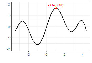
(c)

Figure 9: The function images corresponding to the respective Cases 1-3 of Subsection 5.1 with their global maxima (red points).

We investigate the performance of our SMCO with random sampling points by using two uniform distributions: Unif(-3.16,-3.16+$\alpha$) and Unif(2.37-$\alpha$, 2.37). For comparison, the left and right initial points of GDA are chosen to be -3.16 and 2.37, respectively, with the stepsize $\alpha$ and the iterative points are obtained by

$$x_{j}\leftarrow x_{j}+\alpha f^{\prime}(x_{j}),j=1,\cdots,n.$$ [5.11]

To save space, Figures 10 and 11 below report the comparison for Case 1 function optimization only, as the comparison patterns for other cases are similar. In particular, Figure 10 elucidates the SMCO pattern of alternatively and randomly sampling the points $\{\bm{Z}_{i}^{\bm{\theta}^{*}}:1\leq i\leq n\}$ from the two uniform distributions under $n=20$ and $\alpha=0.006$, which implies that the strategic mean estimator $S_{n}^{\bm{\theta}^{*}}/n$ can attain the global maxima (see Figures 11 below). Figure 10 also shows that, while our SMCO algorithm is robust to the initial values, the track of iterative points of GDA is susceptible to selecting initial values.

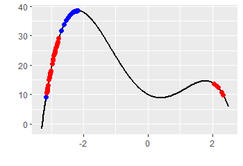
(a)

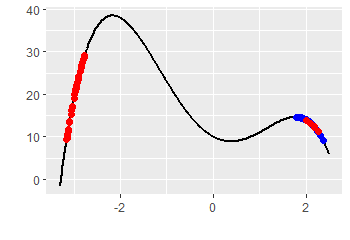
(b)

Figure 10: The randomly sampled points $\bm{Z}_{i}^{\theta^{*}}$ in [2.2] via the developed SMCO (red points), and the iterative points $x_{j}$ in [5.11] by the GDA (blue points) under the left (the left panel) and the right (the right panel) initial points with iterative number $n=20$ and stepsize $\alpha=0.006$ based on the function of Case 1 of Subsection 5.1 after one replicate.

1 Input: Function $f$, Accuracy $\varepsilon$, Min iteration $m$, Max iteration $M$, Exploration weight $C$.

2 Output: Maximum.

3

4Initialize: Generate a tree with only root node $s_{0}$ whose node coordinate $\bm{x}(s_{0})=(\frac{X_{1,1}+Y_{1,1}}{2},\frac{X_{2,1}+Y_{2,1}}{2},\ldots,\frac{X_{d,1}+Y_{d,1}}{2})$, node layer $L(s_{0})=2$ and node exploration $N(s_{0})=0$, $n=0$, Previous maximum = $-\infty$, Maximum = $-\infty$.

5while $(n\leq m)$ or $(n\leq M$ and $\left|\rm{Previous}\ \rm{maximum}-\rm{Maximum}\right|>\varepsilon)$ do

6    $n\leftarrow n+1$

7    Previous maximum $\leftarrow$ Maximum

8    $v\leftarrow$ Selection$(s_{0})$

9    $\rm{Maximum}\leftarrow\max\{Maximum,\text{rollout}$$(v)\}$

10    Backpropagation$(v)$

11 end while

12end

13return Maximum

14 function Expansion$(v)$

15  add two new children $v_{1}^{\prime}$ and $v_{2}^{\prime}$ to $v$

16   with $\bm{x}(v_{1}^{\prime})\leftarrow[L(v)\cdot\bm{x}(v)+(X_{1,N(s_{0})+1}X_{2,N(s_{0})+1},\ldots,X_{d,N(s_{0})+1})]/(L(v)+1)$

17   $\bm{x}(v_{2}^{\prime})\leftarrow[L(v)\cdot\bm{x}(v)+(Y_{1,N(s_{0})+1}Y_{2,N(s_{0})+1},\ldots,Y_{d,N(s_{0})+1})]/(L(v)+1)$

18   $N(v_{1}^{\prime})\leftarrow 0,N(v_{2}^{\prime})\leftarrow 0$

19   $Q(v_{1}^{\prime})\leftarrow 0,Q(v_{2}^{\prime})\leftarrow 0$

20   and $L(v_{1}^{\prime})=L(v_{2}^{\prime})=L(v)+1$

21  return $v_{1}^{\prime}$

22 function Bestchild$(v)$

23  $s\leftarrow\underset{v^{\prime}\in\text{children of }v}{\text{argmax}}{Q(v^{\prime})}+C\sqrt{\frac{\log N(v)}{N(v^{\prime})}}$

24  return $s$

25 function Selection$(v)$

26  while $v$ is not a leaf node do

27   $v\leftarrow\rm{Bestchild}$$(v)$

28  If $N(v)\neq 0$ then

29   $v\leftarrow\rm{Expansion}$$(v)$

30  return $v$

31 function Backpropagation$(v)$

32  $s\leftarrow v$

33  while $v$ is not root node do

34   $N(v)\leftarrow N(v)+1$

35   $Q(v)\leftarrow[(N(v)-1)\cdot Q(v)+\rm{rollout}$$(s)]/N(v)$

36   $v\leftarrow$ parent of $v$

Algorithm 2 SMCO with tree search

We calculate the MSE by averaging 500 replicates of $(S_{n}^{\bm{\theta}^{*}}/n-x^{*})^{2}$ and $(x_{n}-x^{*})^{2}$ for our SMCO (red lines) and the GDA (blue lines), respectively, in Figure 11 for Case 1, where $x^{*}={\rm argmax}_{\underline{\mu}\leq x\leq\overline{\mu}}f(x)$. Multiple SMCO (red) and GDA (blue) MSE lines are plotted for different $\alpha\in[0.2,0.4]$ (different stepsizes in GDA, or equivalently, different lengths of the uniform distributions in SMCO). The fact that the calculated MSE values of the red lines always approximate zero in both the left and right panels implies that our SMCO is independent of the initial points. The GDA method is sensitive to the selection of initial points and steps. In particular, Figure (11(b)) shows that, regardless of the stepsizes, GDA under the right initial point does not converge to the global maximum point $x^{*}$ for the Case 1 function. Other simulated attempts report the Monte Carlo frequencies (across 500 replications) of SMCO and GDA that attain the correct global maxima across different stepsizes $\alpha$ (the lengths of uniform distribution), which shows that the GDA under the left initial points (which are good starting points for the Case 1 function) can take the iterative value to the global maxima under proper stepsize and number of iterations. Still, the GDA under the right initial points never attains the correct global maxima across all considered stepsizes $\alpha\in[0.001,0.005]$ regardless of which accuracy levels to choose. Nevertheless, the proposed SMCO algorithm attends the global maxima with 100% percentage under the considered accuracy level $|x_{m}-x_{m-1}|<10^{-7}$ regardless of which initial points to select, and our SMCO method is robust to the length of uniform distribution (i.e., $\alpha\in[0.001,0.005]$, denoting the variance of the distributions) and achieves low computational complexity with little samplings numbers for attendance of global maxima.

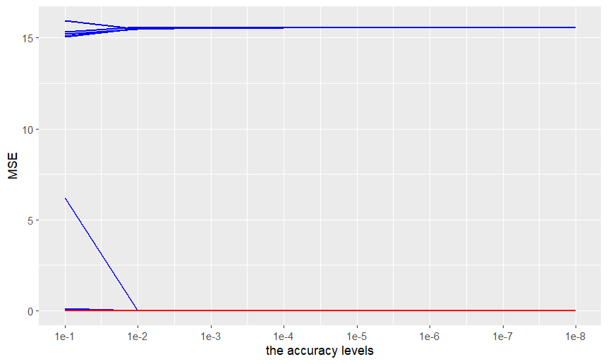
(a)

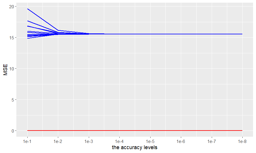
(b)

Figure 11: The averaged MSE after 500 replicates across different accuracy levels $\varepsilon$ with $|x_{m}-x_{m-1}|<\varepsilon$ to stop the iterations/samplings (horizontal ordinate) and distinct stepsizes/lengths of uniform distribution $\alpha$ (multiple lines with $\alpha\in[0.005,0.075]$) via the proposed SMCO (red lines) and the GDA (blue lines) algorithms in Case 1 of Subsection 5.1, where GDA algorithm is implemented under the left (the left panel) and the right (the right panel) initial points respectively.

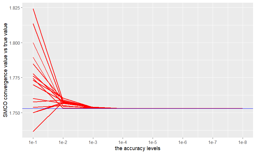
(a)

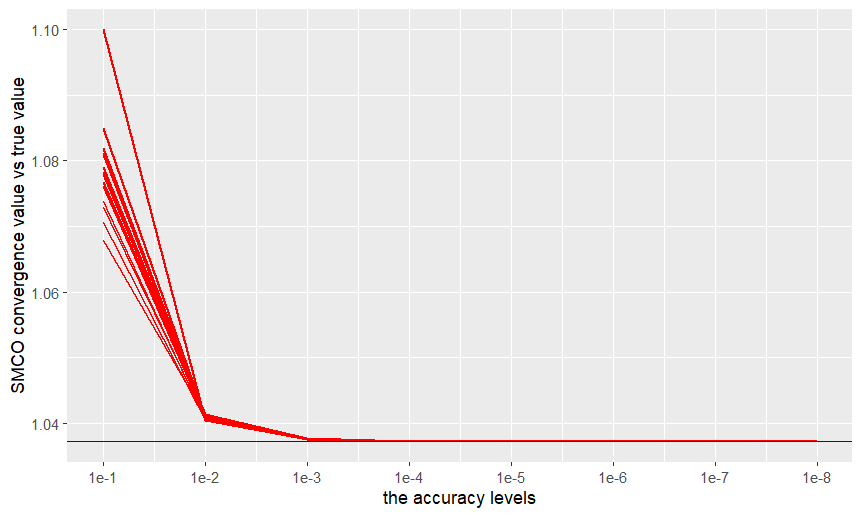
(b)

Figure 12: SMCO convergence values across different accuracy levels $\varepsilon$ (horizontal ordinate) with $|x_{m}-x_{m-1}|<\varepsilon$ to stop the samplings and distinct lengths of uniform distribution $\alpha$ (16 red lines with $\alpha\in[0.05,0.2]$) for Case 2 (the left panel) and $\alpha\in[0.1,0.5]$ for Case 3 (the right panel) in Subsection 5.1.

As a robustness check, Figure 12 below reports the performance of our proposed SMCO estimators (red lines) approaching the true global maximum solutions ($x^{*}$ the blue straight line) across different accuracy levels $\varepsilon$ (horizontal ordinate) with $|x_{m}-x_{m-1}|<\varepsilon$ for Case 2 (Figure 12(a)) and Case 3 (Figure 12(b)), where the multiple red lines are plotted along with varying variances of uniform distributions, i.e.,. For the tall-narrow function in Case 2 with the global maximum value achieved in a narrow region, we choose a minor variance of the uniform distribution with, and then that for the non-convex function in Case 3, where these simulated designs choose $\alpha\in[0.05,0.2]$ and two uniform distributions Unif(0,0+$\alpha$) and Unif(7-$\alpha$, 7) for Case 2, $\alpha\in[0.1,0.5]$ and two uniform distributions Unif(-3.3,-3.3+$\alpha$) and Unif(4.5-$\alpha$, 4.5) for Case 3 respectively. Both figures show that our SMCO algorithms are not sensitive to the varying selections (variances) of uniform distributions and also imply the low computational complexity of our proposed SMCO because it uses a relatively small accuracy level to approach the true global maximum, such as under the accuracy level $10^{-3}$.

5.2 Set identification

This example corresponds to the missing data design of Example 1 presented by Chen et al. (2018) and we use the proposed SMCO optimizer to estimate the parameter set of $\mu$ and the point-identified parameter $\eta_{2}$ by the population form of log-likelihood:

$$f(x)= {\rm E}\left[p_{x}(d,yd)\right]={\rm E}(yd)\log\left[\mu-\eta_{1}(1-\eta_{2})\right]+{\rm E}(d-yd)\log\left[\eta_{2}-\mu+\eta_{1}(1-\eta_{2})\right]$$

$$+{\rm E}(1-d)\log\left[1-\eta_{2}\right]$$

and the parameter space for $x$ is given by $\mathcal{X}=\left\{\left(\mu,\eta_{1},\eta_{2}\right)\in[0,1]^{3}:0\leq\mu-\eta_{1}\left(1-\eta_{2}\right)\leq\eta_{2}\right\}$, where $x=(\mu,\eta_{1},\eta_{2})^{\top}$, ${\rm E}(d)=0.8$ and ${\rm E}(yd)=0.4$.

1 Input: Function $f$, Accuracy $\varepsilon$, Sample sums: $S_{1}^{\bm{\theta}^{a}}=S_{1}^{\bm{\theta}^{b}}=0\in\mathbb{R}^{d}$.

2 Output: $f\left(\frac{S_{n}^{\bm{\theta}^{a}}}{n}\right)$, $f\left(\frac{S_{n}^{\bm{\theta}^{b}}}{n}\right)$.

3

4for $n=1$ to $\infty$ do

5    for $j=1$ to $d$ do

6      

7      if $\partial_{x_{j}}f\left(\frac{S_{n}^{\bm{\theta}^{a}}}{n}\right)>0$ then

8          Draw sample from arm $X_{j}$ (larger mean) ;

9       end if

10      else

11          Draw sample from arm $Y_{j}$ (smaller mean);

12       end if

13      

14      if $\partial_{x_{j}}f\left(\frac{S_{n}^{\bm{\theta}^{b}}}{n}\right)\geq 0$ then

15          Draw sample from arm $X_{j}$ (larger mean) ;

16       end if

17      else

18          Draw sample from arm $Y_{j}$ (smaller mean);

19       end if

20      

21      Allocate the current component $Z_{n+1,j}^{\bm{\theta}^{a}}$ and $Z_{n+1,j}^{\bm{\theta}^{b}}$

22    end for

23   

24   Update $\bm{Z}_{n+1}^{\bm{\theta}^{a}}=(Z_{n+1,1}^{\bm{\theta}^{a}},\cdots,Z_{n+1,d}^{\bm{\theta}^{a}})~,~~\bm{Z}_{n+1}^{\bm{\theta}^{b}}=(Z_{n+1,1}^{\bm{\theta}^{b}},\cdots,Z_{n+1,d}^{\bm{\theta}^{b}})~~,$ and  $S_{n+1}^{\bm{\theta}^{a}}=S_{n}^{\bm{\theta}^{a}}+\bm{Z}_{n+1}^{\bm{\theta}^{a}}$, $S_{n+1}^{\bm{\theta}^{b}}=S_{n}^{\bm{\theta}^{b}}+\bm{Z}_{n+1}^{\bm{\theta}^{b}}$.

25 end for

26

27end for if $\left|\left(\frac{S_{n}^{\bm{\theta}^{a}}}{n}\right)-f\left(\frac{S_{n+1}^{\bm{\theta}^{a}}}{n+1}\right)\right|+\left|f\left(\frac{S_{n}^{\bm{\theta}^{b}}}{n}\right)-f\left(\frac{S_{n+1}^{\bm{\theta}^{b}}}{n+1}\right)\right|\leq 2\varepsilon$.

Algorithm 3 SMCO: Strategic Monte Carlo Optimization for set estimation

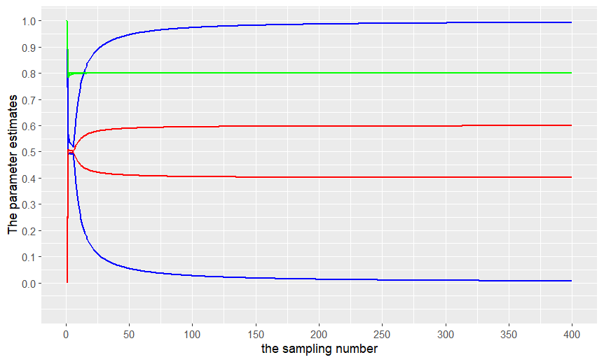
Figure 13: The recovery of the left and right points for the sets of $\mu\in[0.4,0.6]$ (two red lines) and the sets of $\eta_{1}\in[0,1]$ (two blue lines) under the developed two strategies in the Algorithm 3, and the parameter $\eta_{2}=0.8$ (two green lines) can be point-identified consistently because two green lines approximate each other to the true value 0.8 after 400 sampling numbers $n$.

For this example, Figure 13 illustrates the set estimation results for $\mu$, $\eta_{1}$, and $\eta_{2}$ across the iterative number, which indicates that the proposed SMCO algorithm can consistently recover the left and right points of the sets of $\mu$ [0.4, 0.6] (red line) and the sets of $\eta_{1}$ [0, 1] (blue line) under the developed two strategies in the Algorithm 3. Meanwhile, the parameter $\eta_{2}$ can be point-identified consistently because the estimations approximate each other with 0.79 and 0.8 under the left and right point search strategies, respectively.

Data Availability

There are no data underlying this work.

Code availability

The DAQ program is freely available for academic use from Github at
https://github.com/yanxiaodong128/datareconstruction.

Acknowledgements.

This work was supported in part by the National Key R$\&$D Program of China (Grant No. 2018YFA0703900, 2023YFA1008701), the National Natural Science Foundation of China (Grant No. 12371292, 11901352, 12371148) and the Shandong Provincial Natural Science Foundation, China (Grant No. ZR2019ZD41, ZR2022QA063).

References

- [1] Agrawal, R. (1995) Sample mean based index policies with regret for the multi-armed bandit problem. Advances in Applied Mathematics, vol. 27, 1054–1078.
- [2] Bengio, Y., Simard, P. and Frasconi, P. (1994). Learning long-term dependencies with gradient descent is difficult.IEEE transactions on neural networks, 5(2), 157-166.
- [3] Brooks S. P. and Morgan B. J. T. (1995) Optimization Using Simulated Annealing Journal of the Royal Statistical Society. Series D (The Statistician), 44(2), 241-257.
- [4] Browne, C. B., Powley, E., Whitehouse, D., Lucas, S. M., Cowling, P. I., Rohlfshagen, P., and Colton, S. (2012). A survey of monte carlo tree search methods. IEEE Transactions on Computational Intelligence and AI in games, 4(1), 1-43.
- [5] Bubeck, S., and Cesa-Bianchi, N. (2012). Regret analysis of stochastic and nonstochastic multi-armed bandit problems. Foundations and Trends in Machine Learning, 5(1), 1-122.
- [6] Chen, Z., Epstein, L.G., and Zhang, G. (2024). Approximate optimality and the risk/reward tradeoff given repeated gambles. Economic Theory. https://doi.org/10.1007/s00199-024-01614-4.
- [7] Eberhart, R.C. and Kennedy, J. (1995). A new optimizer using particle swarm theory. Proceedings of the 6th international symposium on micromachine and human science, Nagoya, Japan, March 13-16, (pp.39-43), IEEE.
- [8] Fang, X. , Peng, S. , Shao, Q. M. , and Song, Y. (2019). Limit theorems with rate of convergence under sublinear expectations. Bernoulli, 25(4A), 2564–2596.
- [9] Gelly S. and Wang Y. (2006). Exploration exploitation in go: UCT for Monte-Carlo go. In NIPS: Neural Information Processing Systems Conference On-line trading of Exploration and Exploitation Workshop.
- [10] Gittins, J., Glazebrook, K., and Weber, R. (2011). Multi-Armed Bandit Allocation Indices. Second Edition. John Wiley and Sons, Chichester.
- [11] Guo, P., and Fu, M. C. (2022). Bandit-Based Multi-Start Strategies for Global Continuous Optimization. In 2022 Winter Simulation Conference (WSC), 3194-3205 IEEE.
- [12] Hazan, E., Levy, K., and Shalev-Shwartz, S. (2015). Beyond convexity: Stochastic quasi-convex optimization.Advances in neural information processing systems, 28.
- [13] Hinton, G., Srivastava, N., and Swersky, K. (2012). Neural networks for machine learning lecture 6a overview of mini-batch gradient descent.
- [14] Hu, J., Fu, M. C., and Marcus, S. I. (2007). A model reference adaptive search method for global optimization. Operations research, 55(3), 549-568.
- [15] Hu, M., Li, X., and Li, X. (2021) Convergence rate of Peng’s law of large numbers under sublinear expectations. Probability, Uncertainty and Quantitative Risk, 2021, 6(3): 261-266.
- [16] Kennedy, J., and Eberhart, R. (1995). Particle swarm optimization. In Proceedings of ICNN’95-international conference on neural networks (Vol. 4, pp. 1942-1948). IEEE.
- [17] Kingma, D. P., and Ba, J. (2014). Adam: A method for stochastic optimization. arXiv preprint arXiv:1412.6980.
- [18] Kirkpatrick, S., Gelatt Jr.,C. D. and Vecchi, M. P. (1983) Optimization by simulated annealing. Science 221, 671-680
- [19] Krylov, N. V. (1987). Nonlinear parabolic and elliptic equations of the second order. Reidel, Moscow.
- [20] Leprêtre, F., Teytaud, F., and Dehos, J. (2017). Multi-armed bandit for stratified sampling: Application to numerical integration. In Proceedings of the 2017 Conference on Technologies and Applications of Artificial Intelligence (TAAI), (pp. 190–195). IEEE.
- [21] Lai, T. L., and Robbins, H. (1985). Asymptotically efficient adaptive allocation rules. Advances in applied mathematics, 6(1), 4-22.
- [22] Li, X., Lin, K. Y., Li, L., Hong, Y., and Chen, J. (2023). On faster convergence of scaled sign gradient descent. IEEE Transactions on Industrial Informatics, 20(2), 1732-1741.
- [23] Liang, F. (2011). Annealing evolutionary stochastic approximation Monte Carlo for global optimization. Statistics and Computing, 21, 375-393.
- [24] Morokoff, W. J., and Caflisch, R. E. (1995). Quasi-Monte Carlo integration. Journal of Computational Physics, 122(2), 218–230.
- [25] Moulay, E., Léchappé, V., and Plestan, F. (2019). Properties of the sign gradient descent algorithms. Information Sciences, 492, 29-39.
- [26] Owen, A. B. (2013). Monte Carlo Theory, Methods and Examples. Available at: https://artowen.su.domains/mc/.
- [27] Pascanu, R., Mikolov, T., and Bengio, Y. (2013, May). On the difficulty of training recurrent neural networks. In International conference on machine learning. (pp. 1310-1318). PMLR.
- [28] Peng, S. (2019). Nonlinear Expectations and Stochastic Calculus under Uncertainty: with Robust CLT and G-Brownian Motion. Springer Nature.
- [29] Robbins, H. (1952). Some aspects of the sequential design of experiments. Bulletin of the American Mathematical Society, 58(5), 527-535.
- [30] Reddi, S. J., Kale, S., and Kumar, S. (2019). On the convergence of adam and beyond. arXiv preprint arXiv:1904.09237.
- [31] Safaryan, M., and Richtárik, P. (2021). Stochastic sign descent methods: New algorithms and better theory. In International Conference on Machine Learning (pp. 9224-9234). PMLR.
- [32] Yong, J. and X.Y. Zhou (1999). Stochastic Controls: Hamiltonian Systems and HJB Equations (vol. 43). Springer Science Business Media.
- [33] Zeiler, M. D. (2012). Adadelta: an adaptive learning rate method. arXiv preprint arXiv:1212.5701.