UMSPU: Universal Multi-Size Phase Unwrapping via Mutual Self-Distillation and Adaptive Boosting Ensemble Segmenters
Abstract
Spatial phase unwrapping is a key technique for extracting phase information to obtain 3D morphology and other features. Modern industrial measurement scenarios demand high precision, large image sizes, and high speed. However, conventional methods struggle with noise resistance and processing speed. Current deep learning methods are limited by the receptive field size and sparse semantic information, making them ineffective for large size images. To address this issue, we propose a mutual self-distillation (MSD) mechanism and adaptive boosting ensemble segmenters to construct a universal multi-size phase unwrapping network (UMSPU). MSD performs hierarchical attention refinement and achieves cross-layer collaborative learning through bidirectional distillation, ensuring fine-grained semantic representation across image sizes. The adaptive boosting ensemble segmenters combine weak segmenters with different receptive fields into a strong one, ensuring stable segmentation across spatial frequencies. Experimental results show that UMSPU overcomes image size limitations, achieving high precision across image sizes ranging from 256×256 to 2048×2048 (an 8× increase). It also outperforms existing methods in speed, robustness, and generalization. Its practicality is further validated in structured light imaging and InSAR. We believe that UMSPU offers a universal solution for phase unwrapping, with broad potential for industrial applications.
Index Terms:
Phase unwrapping, mutual self-distillation, adaptive boosting, multi-size.I Introduction
Phase unwrapping is a critical technique in fields like structured light imaging[1], synthetic aperture radar[2], and magnetic resonance imaging[3], where phase contains key information. For instance, in structured light imaging and synthetic aperture radar, phase encodes height data[4][5], while in magnetic resonance imaging, it reflects magnetic field uniformity and physiological details[6]. However, phase measurements are often periodic, with phase data wrapped within the range . Phase unwrapping refers to the process of recovering the true phase from the wrapped phase, which is an ill-posed problem since multiple unwrapped phases can correspond to the same wrapped phase. The relationship between unwrapped and wrapped phase can be described as follows:
| (1) |
where is the wrap count at . To obtain a unique unwrapped phase, most methods rely on the phase continuity assumption (Itoh condition)[7], which requires phase differences between adjacent pixels to be less than . However, noise and phase aliasing in practical applications often violate this condition, complicating phase unwrapping.
Conventional phase unwrapping methods recover the true phase by minimizing phase discontinuities. These include the path-following method[8], which uses techniques like branch cuts[9] or quality maps[10] to find optimal paths, and the iterative optimization method[11], which minimizes the difference between unwrapped and wrapped phase gradients[12]. However, the path-following method may generate unreasonable paths for complex wrapped phases, compromising accuracy[13], while optimization methods often produce smooth results that fail in noisy images, where phase differences may not be integer multiples of . Despite mitigating discontinuities, both methods can fail under severe noise or distorted wrapped phases[13], and are too slow for real-time applications.
Recent studies have shown that neural networks can effectively perform phase unwrapping without being restricted by the Itoh condition, even in noisy environments[14]. As a result, deep learning-based phase unwrapping methods have become a research hotspot in the field. The methods include regression method[15], wrap count method[13], and gradient method[16].
The regression method directly maps the wrapped phase to the unwrapped phase using a neural network[17], but the predicted phase often deviates from Eq. (1), limiting accuracy[18].
The wrap count method frames phase unwrapping as a semantic segmentation task, classifying the wrap count for each pixel[13]. This ensures that the wrapped and unwrapped phases satisfy Eq. (1) and is relatively fast, making it widely used[18]. However, it requires a large receptive field to segment the continuous wrap counts, making it ineffective for high-size images and hindering generalization to phases that differ significantly from the training data.
The gradient method classifies the wrap count gradient and reconstructs the unwrapped phase through post-processing[16]. Since it relies only on local features, it alleviates the receptive field limitation, better aligning with the essence of phase unwrapping. However, the sparse distribution of wrap count gradients (mostly 0) causes class imbalance, making network training challenging. This sparsity increases with larger image sizes, limiting the method to low-size images. Additionally, inaccuracies in gradient prediction require complex post-processing, slowing down the unwrapping process and limiting the method’s applicability.
To achieve phase unwrapping under multiple size conditions, we propose a universal multi-size phase unwrapping network (UMSPU) based on Mutual Self-Distillation (MSD) and adaptive boosting ensemble segmenters. MSD enhances shallow-layer perception and refines deep features through bidirectional attention distillation, allowing the network to finely capture semantic information across sizes. The adaptive boosting ensemble segmenters combine multiple weak segmenters with varying receptive fields into a strong one, ensuring stable segmentation of semantic information at different spatial frequencies. With these two components, the network achieves high-precision wrap count gradient segmentation, and the unwrapped phase is reconstructed through a post-processing method based on discrete cosine transform. Our main contributions are summarized as follows:
-
•
We propose a novel mutual self-distillation (MSD) mechanism based on bidirectional feature refinement between the encoder and decoder. During training, MSD leverages feature attention maps from corresponding layers of the encoder and decoder as mutual distillation targets, optimizing bidirectional Kullback-Leibler (KL) divergence. This process provides cross-layer supervision, enabling dynamic interaction between shallow and deep representations. Cross-layer learning enhances the discriminative power of low-level features and refines high-level details, ensuring stable semantic extraction across sizes and effectively addressing spatial and semantic variability within a unified framework.
-
•
We construct a multi-scale ensemble segmentation architecture using an adaptive boosting strategy. It integrates three sub-segmenters with different receptive field sizes, enabling the system to process spatial features at various scales. During training, their weights are optimized iteratively, forming a strong segmenter that adapts to a wider range of spatial frequencies, effectively mitigating frequency bias and ensuring precise, generalized semantic segmentation.
-
•
Experimental results demonstrate that UMSPU overcomes size limitations, achieving precise phase unwrapping across sizes from 256×256 to 2048×2048. It also shows significant advantages in robustness, generalization, and speed, highlighting its potential for practical application in real-world measurement scenarios.
II RELATED WORK
II-A Deep Learning in Phase Unwrapping
The application of deep learning to phase unwrapping has seen significant progress in recent years. It offers new solutions to complex problems that conventional methods struggle to address. Deep learning-based phase unwrapping methods mainly include regression method, wrap count method, and gradient method.
II-A1 Regression Method
This method constructs regression models to map the wrapped phase to the unwrapped phase. Yair Rivenson et al. applied convolutional neural networks (CNNs) for holographic phase unwrapping, significantly accelerating holographic image reconstruction due to the high-speed inference of deep learning[17]. However, the regression-based unwrapped phase often fails to satisfy Eq. (1), introducing errors. To address this, L. Zhou et al. proposed a conditional generative adversarial network with the norm for one-step phase unwrapping[18], which partially reduced phase ambiguity and inconsistency. Nonetheless, this method struggles with input sizes different from the training set, leading to unreliable results.
II-A2 Wrap Count Method
G. E. Spoorthi et al. first reformulated phase unwrapping as a semantic segmentation problem and introduced PhaseNet, which classifies the wrap count for each pixel to achieve phase unwrapping[14]. PhaseNet2.0 improved on PhaseNet with enhanced loss functions and model structures, achieving better accuracy and noise resistance[13]. The wrap count method is fast and satisfies the constraints of Eq. (1). However, wrap count classification relies on global feature integration, requiring a large receptive field. This limits its effectiveness to low-size images, with PhaseNet and PhaseNet2.0 only performing well at 256×256 size. Zhang et al. employed spatial pyramid pooling and positional self-attention to expand feature extraction to larger spatial ranges, achieving higher accuracy and robustness[19]. However, this approach still struggled with high-size image processing.
II-A3 Gradient Method
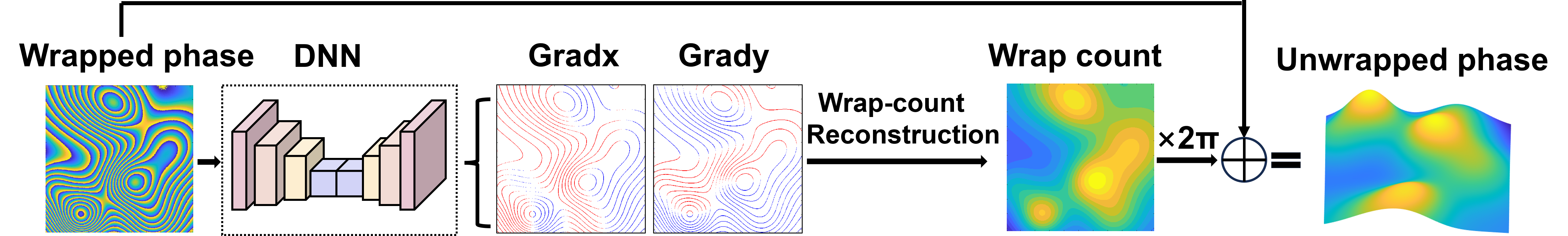
L. Zhou et al. proposed PGNet, which classifies the wrap count gradient at each point and uses an optimization algorithm to recover the unwrapped phase[16], as shown in Figure 1. Wrap count gradient prediction relies on local features and requires a smaller receptive field, but it is inherently sparse, with +1 or -1 categories constituting a small fraction of the image[20]. This severe class imbalance worsens at higher sizes, making gradient segmentation networks difficult to train for high-size images. PGNet demonstrated phase unwrapping only at 64×64 size. F. Sica et al.[21] and H. Wang et al.[20] incorporated interferometric coherence and quality maps as additional inputs, increasing size to 128×128. Gao et al. extended size to 256×256 with an improved LinkNet featuring a pretrained encoder and dilated convolutions[22]. However, this method relied on a complex unscented Kalman filter for post-processing, which was time-consuming and unsuitable for real-time phase unwrapping.
II-B Self-Distillation for Performance Improvement
Distillation in neural networks is a model compression and optimization technique aimed at improving the performance of a smaller student network by transferring knowledge from a larger teacher network. First proposed by Hinton et al., this method leverages ‘soft labels’, or the predicted probability distributions from the teacher network, as training targets for the student network[23]. This enables the student network to learn both accurate classifications and richer inter-class relationships. For instance, S. Chen et al. introduced a nonlinear weight-sharing mapping mechanism for distillation, successfully applying it to facial attribute recognition while reducing computational and memory costs[24].
Self-distillation, a variant of distillation, uses the same network as both teacher and student at different training stages or within the same process. Its key advantage is eliminating the need for an external teacher network, relying on self-guidance to enhance accuracy, generalization, and robustness across tasks. H. Chen et al. developed a self-distillation paradigm for fine-tuning in few-shot object detection, mitigating misalignment between learned and actual distributions[25]. K. Xu et al. proposed a feature-enhanced self-distillation method based on feature extrapolation, demonstrating its effectiveness across modalities for classification tasks[26].
II-C Ensemble Learning
Ensemble learning combines predictions from multiple models to leverage their strengths and mitigate individual weaknesses, achieving more accurate and generalized results. Ensemble strategies include Bagging[27], Boosting[28], and Stacking[29].
Bagging (Bootstrap Aggregating)[27] creates multiple training subsets via resampling, trains models on these subsets, and combines their predictions. For example, Random Forest[30], proposed by L. Breiman, applies Bagging to decision trees. Bühlmann and Yu explained Bagging’s ability to stabilize decisions, reduce variance, and minimize mean squared error[31]. Y. Sun et al. extended Bagging to video recognition by integrating subnetworks with alternating residual links, forming an ensemble network[32]. Boosting improves weak learners by iteratively training new models on previous errors, enhancing overall performance. Notable methods include AdaBoost[28] and Gradient Boosting[33]. AdaBoost minimizes classification error using a greedy approach to produce weighted predictors. Gradient Boosting generalizes AdaBoost to differentiable loss functions. M. Saldanha et al. employed Gradient Boosting for Versatile Video Coding, training classifiers on texture, coding, and context features[34]. Stacking, introduced by D. H. Wolpert, combines diverse base models using a meta-learning model to reduce bias[29]. Predictions from base models are combined by the meta-learner for improved performance. Y. Wei et al. proposed a data-free meta-learning approach using diffusion models to address data scarcity in few-shot learning[35].
III METHOD
III-A Overview
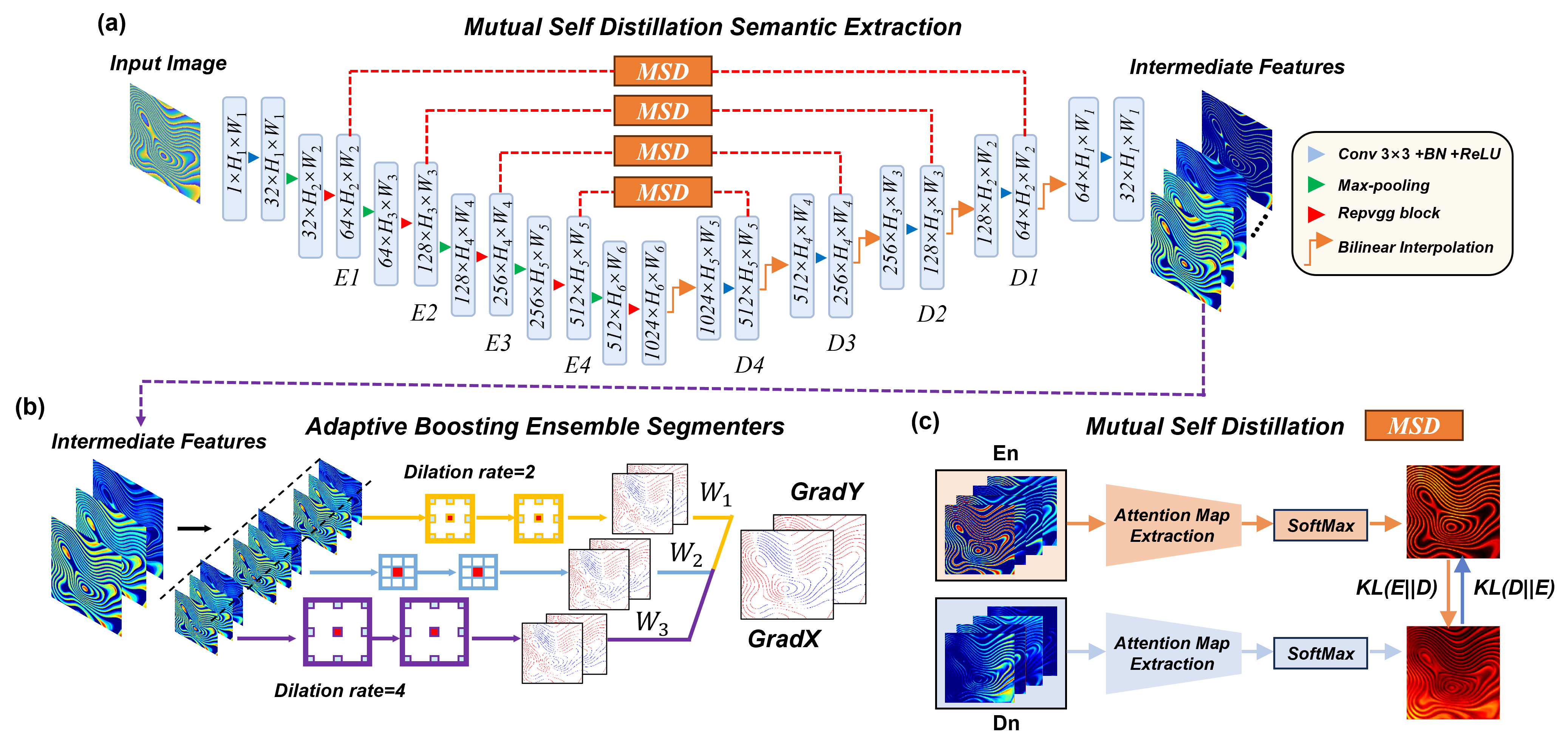
As shown in Fig. 2, we propose a cross-size phase unwrapping network, UMSPU, which performs pixel-level wrap count gradient prediction. UMSPU consists of two components: (a) semantic information extraction and (b) segmenter. In (a), to stably and effectively extract semantic information from cross-size images, we introduce a Mutual Self-Distillation (MSD) mechanism. By performing attention distillation between the encoder and decoder during training, MSD effectively enhances the perceptual ability of shallow layers and strengthens the expression of detailed information in deep layers. The spatial frequency of semantic features extracted by the network changes with size. To address this issue, we design an ensemble architecture segmenter at the network’s end in (b). Using adaptive boosting, three segmenters with different receptive fields are weighted and combined into a robust segmenter, covering a broader range of spatial frequencies, enabling precise segmentation across cross-size images. Additionally, we design a weighted loss function and a curl loss function to improve training accuracy while ensuring the physical constraints of a curl-free field are satisfied.
III-B Mutual Self-Distillation
The wrap count gradient is classified into +1, 0, and -1, with pixels of ±1 being highly sparse. This sparsity increases at higher sizes, challenging the encoder-decoder architecture in cross-size processing. In low-size inputs, sparse semantic information diminishes through network layers, leading to blurred stripe features and reduced gradient segmentation accuracy[36]. In high-size inputs, capturing sparse semantic information requires broader feature perception, but shallow layers, constrained by small receptive fields, struggle to capture the long-range context necessary for locating stripe edges. This disrupts high-level feature propagation and hampers the recovery of sparse semantic cues, resulting in cumulative errors in stripe edge localization[37].
To enable UMSPU to adapt to cross-size inputs and capture sparse semantic features effectively, we propose a Mutual Self-Distillation (MSD) mechanism within the encoder-decoder architecture. The core principle of MSD is to promote the exchange of information between shallow and deep layers through two-way distillation learning during network training. Decoder-to-encoder distillation helps the encoder capture the global context of these sparse features more effectively under high-size inputs, enabling the rapid localization of gradient distribution. Encoder-to-decoder distillation mitigates the degradation of sparse information in the deep layers under low-size inputs. Specifically, MSD connects feature maps of the same size in the encoder and decoder during training and distills their corresponding attention maps. The attention maps represent the regions of interest in each network layer and can be calculated from the feature maps as follows:
| (2) |
where and represent the values at in the channel of feature maps from encoder and decoder. Softmax function is then applied along the spatial dimension for normalization, generating the soft attention map labels:
| (3) |
where and represent the height and width of the image. and are the values at in soft attention map labels of encoder and decoder. Subsequently, the bidirectional KL divergence loss is calculated as:
| (4) |
denotes the KL divergence from the encoder’s attention maps to the decoder’s, where the encoder serves as teacher and the decoder as student. Conversely, refers to the divergence in the opposite direction, with the decoder as teacher and the encoder as student. and are the weight coefficients for these two losses. mitigates detail distortion in deep features for low-size inputs. enhances shallow layers’ contextual perception, enabling fine segmentation and dense prediction for high-size images. Therefore, during training, is prioritized for low-size images and for high-size ones. Accordingly, we set the weight coefficients and as follows:
| (5) |
where represents the current image size, and correspond to the preset maximum and minimum sizes. As decreases, the proportion of increases. As increases, the proportion of increases.
As shown in Fig. 2(a), to accelerate the network, we use the RepVGG Block as the basic module in the encoder. The RepVGG Block adopts the concept of structural re-parameterization, converting the multi-branch structure during training into a single-branch structure for inference[38]. This significantly improves inference speed and reduces memory consumption. The detailed principles can be found in reference [38]. As shown in Fig. 2(c), MSD performs attention maps extraction and calculates two-way KL divergence losses for mutual attention distillation.
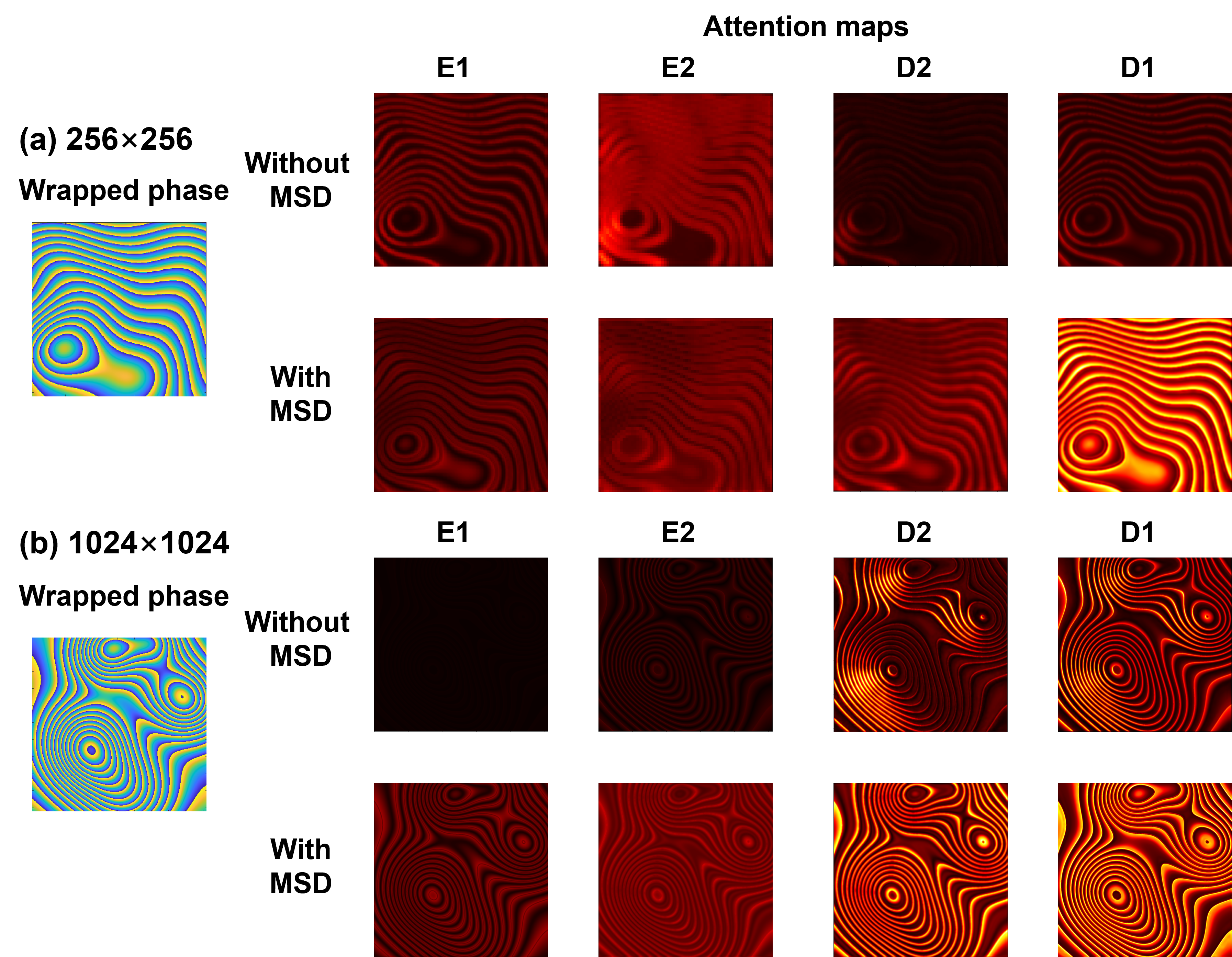
As shown in Fig. 3, we compare the changes in the attention maps of the encoder E1, E2 and the decoder D1, D2 before and after introducing the MSD. Fig. 3(a) shows that after adding MSD, the deeper layers of the network (D1, D2) focus more on the details at the phase cycle boundaries with low-size images of 256×256. This indicates that MSD helps the deep features retain critical details and enhances the recognition of stripes. Fig. 3(b) demonstrates that with high-size images of 1024×1024, the introduction of MSD allows the shallower parts of the network (E1, E2) to direct their focus towards the stripe regions. This suggests that MSD helps the network begin integrating semantic information at earlier stages, allowing it to identify important regions sooner. Additionally, the enhanced attention in E1 and E2 further increases the feature contrast in D2 and D1, improving the network’s ability to distinguish between gradient and non-gradient points, which contributes to better segmentation accuracy in subsequent stages. Overall, MSD helps the network achieve more balanced and efficient semantic information extraction when processing inputs at different sizes.
III-C Adaptive Boosting Ensemble Segmenters
MSD enhances the consistency of semantic information extraction in the network under inputs of different sizes. Due to variations in stripe density and size, the semantic information output by the decoder exhibits diverse spatial frequencies. However, a single segmenter at the end of the network is limited by its fixed convolutional kernel size, making it difficult to adapt flexibly to the various frequency components of the semantic information. This limitation causes the network to excessively depend on and overfit to particular spatial frequency, making it challenging to maintain stable segmentation performance in the presence of varying spatial frequency[39]. To overcome this challenge, we integrate multiple sub-segmenters with different receptive fields, achieving comprehensive coverage and efficient utilization of multi-scale spatial frequency features. As shown in Fig. 2(b), the ensemble segmenter consists of three distinct sub-segmenters, each using a 3×3 convolutional kernel as the base but with different dilation rates of 1, 2, and 4, respectively. This configuration provides the three sub-segmenters with different receptive fields, allowing them to focus on spatial frequency information at different scales.
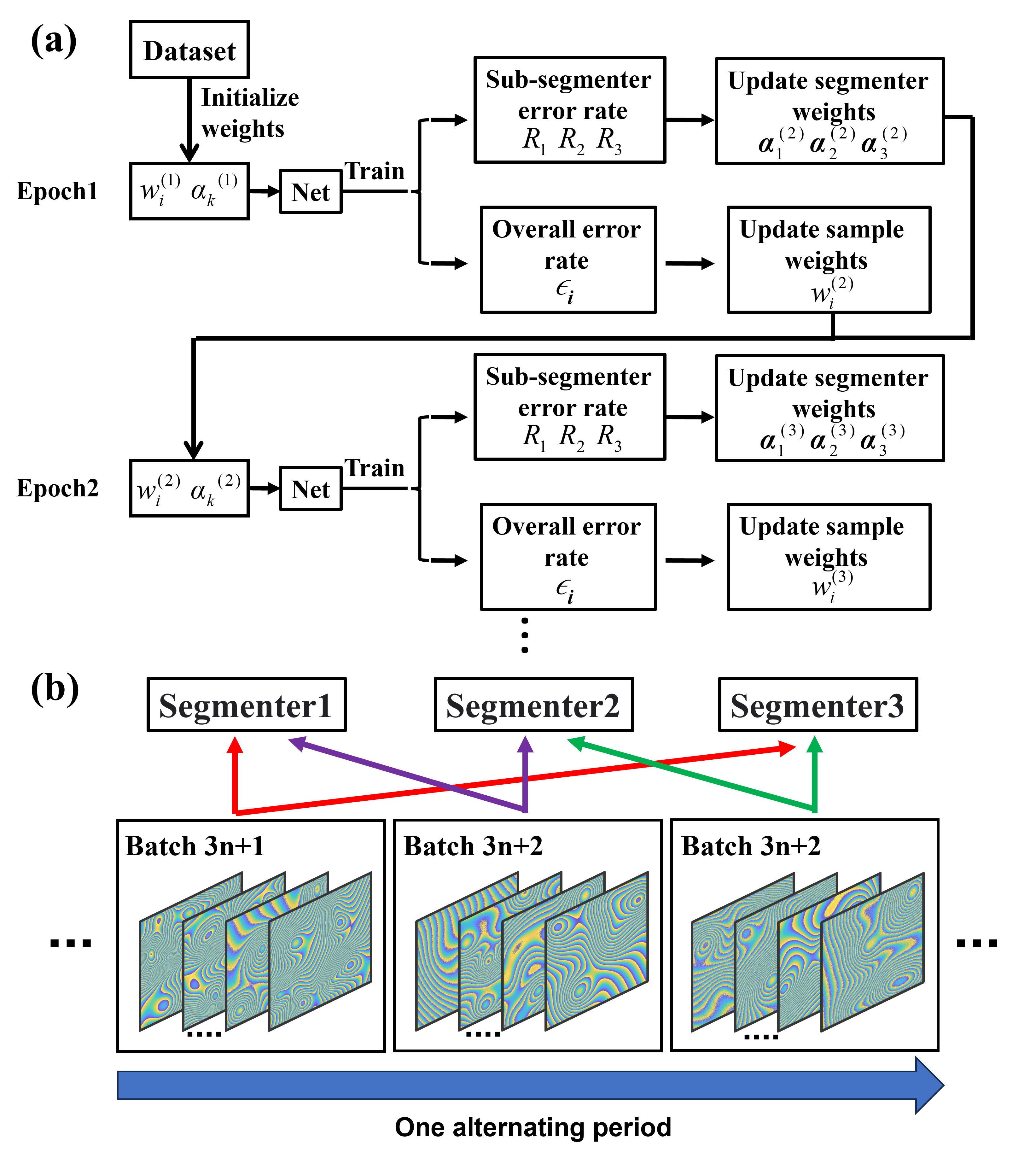
Under the ensemble learning framework, each weak segmenter dynamically adjusts its ability to capture frequency characteristics during the training process. However, due to the lack of clear prior information, it is difficult to assign appropriate weights to each segmenter before training. To ensure as much as possible that the multi-segmenter system achieves the widest and most complementary frequency coverage, we design an algorithm that dynamically updates the weights of each segmenter. Inspired by the Adaboost algorithm, as shown in Fig. 4, we design the specific training process as follows:
Step 1: Dataset Initialization and Cross-Training. To avoid homogenization among the three sub-segmenters, we assign differentiated datasets during training. As shown in Fig. 4(b), We pair every two segmenters, resulting in three training pairs and alternately assign each input batch to a specific pair. This alternate mechanism ensures that each sub-segmenter is exposed to different combinations of sample sets, thereby enhancing its independence and diversity. During training, gradient accumulation is applied, with backpropagation performed every three batches. The encoder-decoder architecture is updated using the accumulated gradients, while each sub-segmenter is updated independently based on its respective gradients.
Step 2: Update the Weights of the Segmenters. As shown in Fig. 4(a), between the adjacent epochs and , we update the weight of the th segmenter from to . This update is based on the error rate of the -th segmenter on the dataset, where higher error rates correspond to smaller weights. Specifically, after each training round, we calculate as a weighted sum of individual sample errors:
| (6) |
where is the total number of samples, and is the weight of the -th sample at epoch , reflecting the difficulty of the sample. Initially, . The term denotes the error rate of the -th segmenter on the -th sample, calculated as:
| (7) |
where is the prediction of the -th segmenter for the -th pixel of the -th image, and is the corresponding ground truth label. The indicator function equals 1 if , and 0 otherwise. For gradient mask points, ; for non-gradient points, . Thus, only errors on gradient mask points are considered.
Finally, based on the error rate , the weight of the -th segmenter is updated using the following formula:
| (8) |
Step 3: Sample Weights Update. To emphasize samples with higher error rates in the next epoch, sample weights are updated accordingly. The pixel error rate of the th image is calculated based on the weighted prediction results of the three segmenters:
| (9) |
where represents the true label of the th pixel in the th image, and is the aggregated result of the three segmenters. The indicator function equals 1 if , and 0 otherwise. Only pixels on the gradient mask (where ) are considered. Using the sample error rate , the sample weights are updated as follows:
| (10) |
where is the weight of the th image at epoch , and is the updated weight for the next epoch. Samples with updated weights below a threshold are discarded, and new samples are introduced to enhance the model’s generalization. The weight for newly introduced samples is set to the mean weight , and all sample weights are re-normalized before the next round of training.
By applying the above method to create a weighted ensemble of the three sub-segmenters, the network covers a broader frequency range, effectively avoiding the spatial frequency bias.
III-D Loss Function
The loss function for wrap count gradient segmentation is designed to address two key challenges: (1) severe class imbalance, as the +1 and -1 classes have significantly fewer points compared to the 0 class, and (2) adherence to the physical constraint that gradient fields must be irrotational[40]. To address these challenges, we propose a loss function that combines a weighted loss to handle class imbalance and a curl loss to enforce the irrotational constraint.
To mitigate the imbalance between classes, we design a weighted loss function, enabling the model to focus more on the segmentation accuracy of the +1 and -1 classes. The weighted loss consists of a weighted mean squared error (MSE) loss and a weighted cross-entropy loss, defined as:
| (11) |
where and denote the weighted MSE and cross-entropy losses, respectively. The one-hot encoded label at point in channel is , and is the corresponding model output after softmax normalization. The weight for the class corresponding to channel is denoted as . Channel 0, 1, and 2 represent the 0, +1, and -1 classes, respectively. , , and denote the number of channels, height, and width of the image.
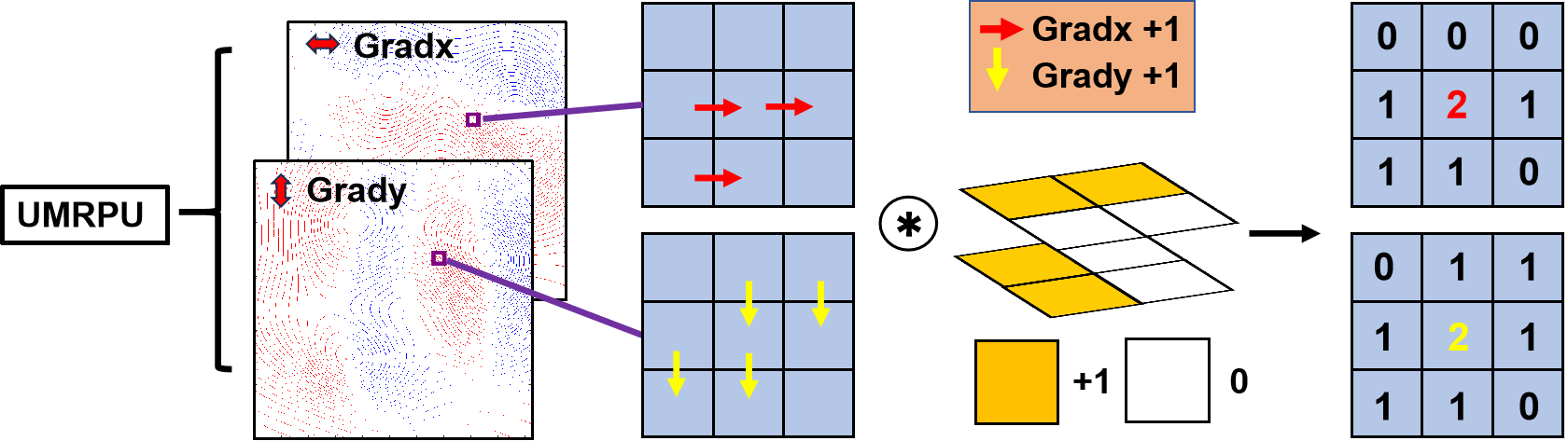
To ensure compliance with the irrotational constraint, we introduce a curl loss. This loss is based on a fixed-weight convolution-based curl estimation method. As shown in Fig. 5, two fixed convolution kernels, and , are applied to detect consecutive gradients in the horizontal and vertical directions:
| (12) |
For gradx, the kernel detects consecutive gradients of ±1 along the horizontal direction, with the convolution result being 2 or -2 at curl points. Similarly, for grady, the kernel detects vertical gradients. Curl points are identified as points with convolution results of 2 or -2. The curl loss is then defined as the ratio of curl points to gradient points:
| (13) |
where and represent the number of curl points and gradient points, respectively.
The loss function for each segmenter is defined as:
| (14) |
where is the loss for the th segmenter, and represents the KL divergence loss from MSD. The total loss for the model is defined as:
| (15) |
where , , and are the weights assigned to segmenter 1, 2, and 3, respectively. By combining these losses, the model effectively balances class-specific accuracy, physical constraints, and multi-segmenter coordination, ensuring robust and consistent gradient segmentation.
III-E Phase Reconstruction
After obtaining the gradients in the x and y directions, we use the least squares algorithm to reconstruct the wrap count gradient into the wrap count. Then, we multiply the wrap count by and add the wrapped phase to obtain the final unwrapped phase.The detailed derivation is provided in the supplementary material.
IV Experiments
This section introduces our experimental framework. Section IV-A details the experimental settings. Section IV-B compares UMSPU with other methods across different sizes, fringe densities, and processing speed. Section IV-C conducts an ablation study to validate the effectiveness of UMSPU’s components. Section IV-D evaluates UMSPU’s stability and generalization under translational and rotational deformations. Finally, Section IV-E and Section IV-F demonstrate UMSPU’s practicality through comparisons in two real-world scenarios: structured light facial reconstruction and Interferometric Synthetic Aperture Radar.
IV-A Experimental Settings
IV-A1 Datasets
Following the method in [13], we generated the unwrapped phase by superimposing multiple Gaussian distributions with varying peaks and standard deviations onto a linear function. The wrapped phase was then computed, and the x- and y-direction wrap count gradients were derived through differentiation to serve as training labels. To generate the model input, noise was added to the unwrapped phase, followed by a four-step phase-shifting process to compute the wrapped phase.
The dataset contains 12,000 samples, split into 80% for training, 10% for validation, and 10% for testing. Sample sizes range from 256×256 to 2048×2048, with SNRs between -2 dB and 4 dB. The network output consists of six channels: the first three represent the horizontal gradient classes, while the last three represent the vertical gradient classes.
IV-A2 Implementations
The network is implemented using PyTorch, with training conducted on an NVIDIA A100 Tensor Core GPU and testing on an NVIDIA GeForce RTX 2060. The network is trained using the SGD optimizer with a batch size of 4, a learning rate of 1e-3, and a weight decay of 5e-4, reaching convergence after 300 epochs. During training, the sample weight threshold in III-C is set to 5e-5. The class weights in III-D are defined as [1, 10, 10], where class 0 is assigned a weight of 1, and classes 1 and -1 are assigned weights of 10.
IV-A3 Evaluation Metrics
Root mean square error (RMSE) is used to evaluate the phase unwrapping performance of the proposed and baseline methods. RMSE is defined as:
| (16) |
where represents the ground truth unwrapped phase at point , is the predicted unwrapped phase, and and are the image height and width, respectively.
IV-B Comparison
To validate the performance of UMSPU, we conducted comparative experiments with six commonly used phase unwrapping networks, including REDN[41], PhaseNet[14], PhaseNet2.0[13], DeepLabv3+[42], VDENet[43], and GAUNet[20]. The comparisons included analyses under different sizes, varying fringe densities, and model computational complexity.
| Size | Method | ||||||
| REDN | PhaseNet | PhaseNet2.0 | DeepLabv3+ | VDENet | GAUNet | UMSPU | |
| 256256 | 0.5185 | 0.6269 | 0.5331 | 0.5427 | 0.4754 | 0.4322 | 0.2954 |
| 512512 | 2.4752 | 5.5155 | 4.1424 | 4.8923 | 2.7527 | 3.3639 | 0.3392 |
| 10241024 | 24.9531 | 41.2977 | 33.2376 | 31.6656 | 25.5948 | 20.3161 | 0.3429 |
| 20482048 | 37.2958 | 44.3165 | 42.2926 | 45.5863 | 39.8346 | 31.4632 | 0.3483 |
IV-B1 Comparison at Different Sizes
We constructed four test sets with sizes of 256×256, 512×512, 1024×1024, and 2048×2048 to evaluate the performance of UMSPU and six other networks. As shown in Table I, all methods achieve low RMSE values at the lowest size (256×256). Among them, UMSPU performs best with a mean RMSE of 0.2954, followed by GAUNet, a gradient-based network, with a mean RMSE of 0.4322. This represents a 31.65% improvement compared to PGNet. As the size increases to 512×512, 1024×1024, and 2048×2048, UMSPU maintains high accuracy with mean RMSE values of 0.3392, 0.3429, and 0.3483, respectively. In contrast, the RMSE of the other six networks increases sharply and remains significantly higher than that of UMSPU.
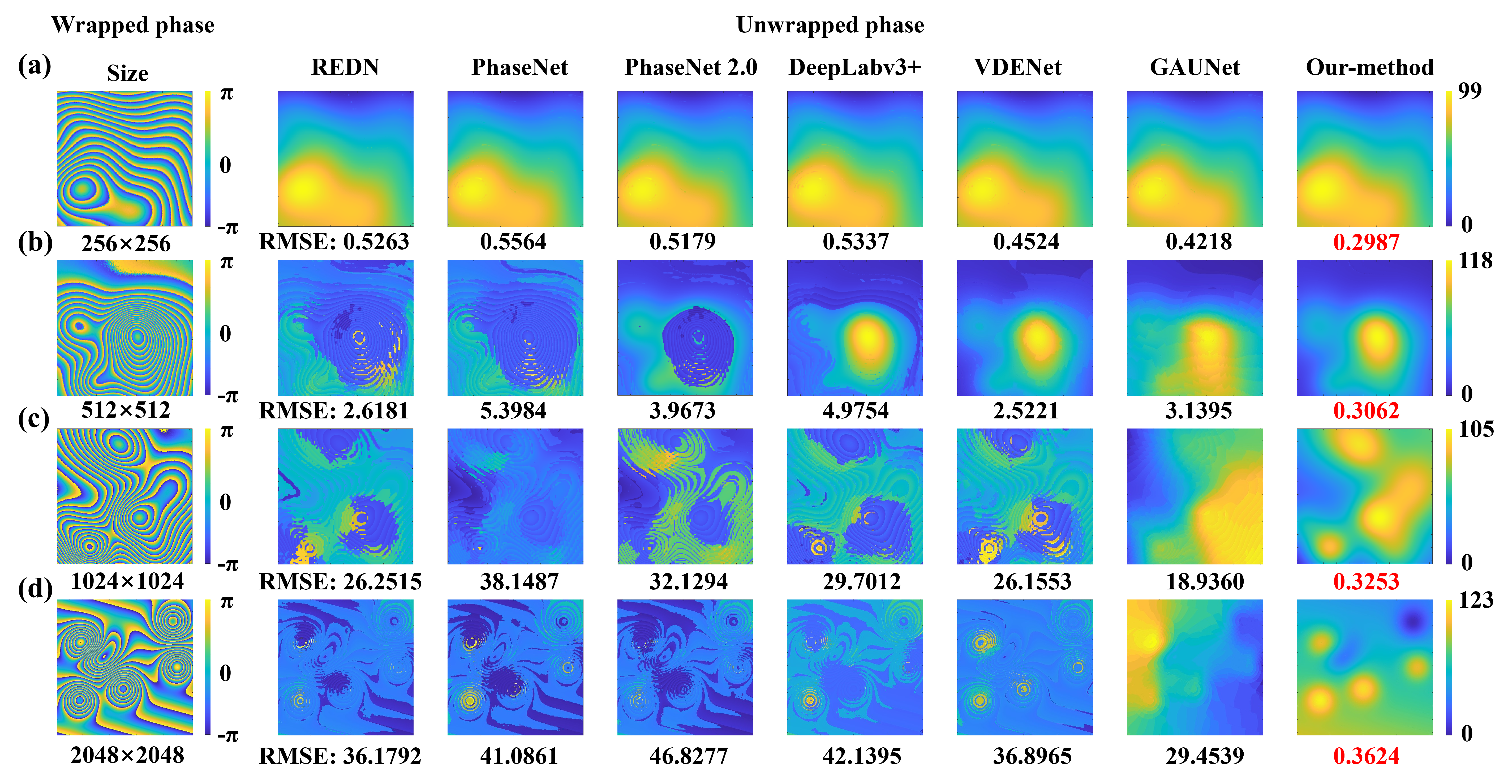
To further illustrate this comparison, we randomly selected one sample from each size for phase unwrapping using all methods. As shown in Fig. 6, the other networks exhibit high accuracy only at the 256×256 size and fail at higher sizes. Specifically, REDN, PhaseNet, and PhaseNet 2.0 (wrap count method), as well as DeepLabv3+ and VDENet (regression method), all produce RMSE values exceeding 35 at higher sizes. This is because both wrap count and regression methods rely heavily on receptive field size. As input image size increases, the receptive fields of these networks fail to capture sufficient contextual information, leading to an inadequate understanding of details and the global structure in large images. GAUNet, as a gradient-based method, is less constrained by receptive field size but struggles with finer and more complex gradient variations at high sizes due to its limitations in extracting complex structural features. This leads to error accumulation and gradient prediction distortion, resulting in RMSE values of 18.9360 and 29.4539 at 1024×1024 and 2048×2048, respectively. In contrast, UMSPU consistently achieves excellent phase unwrapping results across all sizes, with RMSE values of 0.2987, 0.3062, 0.3253, and 0.3624 at the four sizes, respectively. These results indicate that UMSPU overcomes the size limitations in phase unwrapping, showing excellent performance across various sizes.
IV-B2 Comparison at Different Densities
To validate the impact of fringe spatial frequency on network output, we constructed four test sets for the experiment. The images in the test sets all have a size of 1024×1024 but differ in fringe density, specifically 10(3), 30(3), 50(3), and 70(3). We used UMSPU and six other methods on these four test sets and compared their mean RMSE. Notably, since the other six methods are unable to handle high-size images, we adopted an image tiling approach for high-size prediction, where each image is divided into 16 regions of 256×256 pixels, processed individually, and then stitched back to the original size. In contrast, UMSPU directly processes the full image without the need for tiling, thanks to its ability to handle high-size inputs.
| Method | Wrap count | |||
| 10( 3) | 30( 3) | 50( 3) | 70( 3) | |
| REDN | 0.3927 | 0.5669 | 0.9136 | 3.5423 |
| PhaseNet | 0.5477 | 0.6946 | 3.8121 | 13.2215 |
| PhaseNet2.0 | 0.4823 | 0.6370 | 2.4862 | 7.3429 |
| DeepLabv3+ | 0.4731 | 0.5576 | 5.3865 | 9.0873 |
| VDENet | 0.4239 | 0.5174 | 4.1882 | 7.6342 |
| GAUNet | 0.3579 | 0.4634 | 0.8750 | 3.4766 |
| UMSPU | 0.2911 | 0.2957 | 0.3316 | 0.3728 |
As shown in Table II, under lower fringe densities of 10(3) and 30(3), all seven methods successfully perform phase unwrapping. The mean RMSEs of UMSPU are 0.2911 and 0.2957, respectively, while the second-best method, GAUNet, has mean RMSEs of 0.3579 and 0.4634, indicating that our method reduces RMSE by 18.66% and 36.18% compared to GAUNet. Even the worst-performing method, PhaseNet, maintains mean RMSEs of 0.5477 and 0.6946.
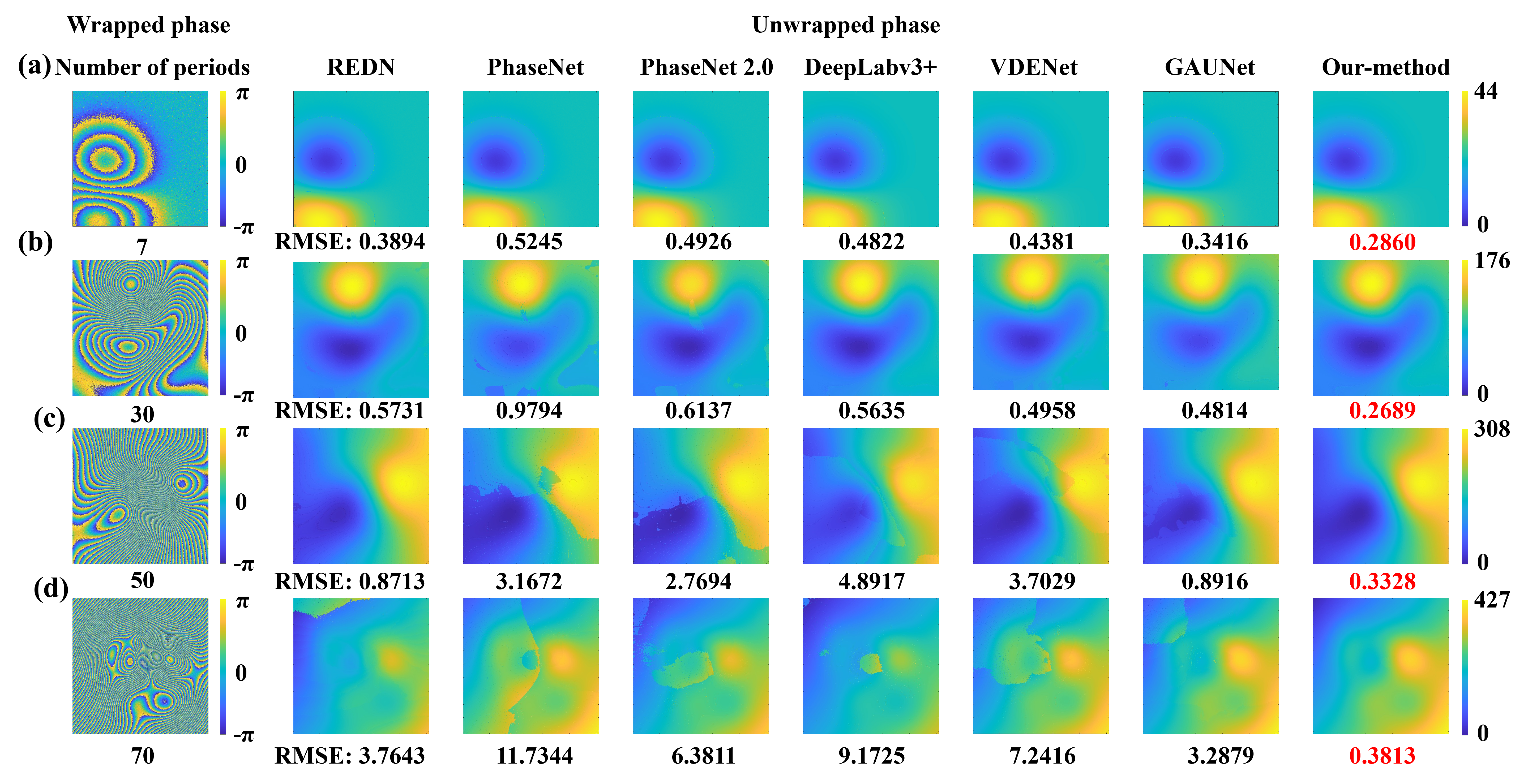
Under higher fringe densities of 50(3) and 70(3), UMSPU still achieves high-precision unwrapping, with mean RMSEs of 0.3316 and 0.3728, while the second-best GAUNet reaches 0.8750 and 3.4766, significantly higher than ours. Additionally, we randomly select one sample from each of the four densities. As shown in Fig. 7, although the RMSE of UMSPU increases slightly with higher fringe densities, it remains as low as 0.3813 even at a fringe density of 70. This demonstrates that UMSPU adapts well to varying fringe densities.
In contrast, the other networks successfully unwrap phase at lower fringe densities of 7 and 30, but fail at densities of 50 and 70. This highlights the superiority of UMSPU in handling phase distributions across various spatial frequencies.
IV-B3 Model Computational Complexity
We compared the computational complexity of UMSPU with six other networks under 1024×1024 resolution input. As shown in Table III, UMSPU has the lowest FLOPs, number of parameters, and inference time among all the networks. This demonstrates that UMSPU has significant advantages in terms of speed and lightweight design, making it easier to apply in real-world scenarios. Despite having the smallest computational complexity, UMSPU still achieves optimal performance, highlighting its efficiency. The efficiency comes from two aspects: first, the MSD mechanism enables the relatively simple network to achieve excellent performance through internal mutual representation learning during training. Second, we employed the RepVGG block as the basic module in the encoder, which uses structural reparameterization to convert the multi-branch topology during training into a single-path structure for inference, greatly optimizing the network’s inference efficiency.
| Method | FLOPS | Params | Inference Time |
| (GFLOPs) | (million) | (ms) | |
| REDN | 951.30 | 17.71 | 756.14 |
| PhaseNet | 495.93 | 13.40 | 321.07 |
| PhaseNet2.0 | 68.22 | 7.97 | 80.25 |
| DeepLabv3+ | 94.97 | 25.40 | 76.30 |
| VDENet | 126.56 | 51.10 | 106.46 |
| GAUNet | 770.83 | 31.04 | 472.32 |
| UMSPU | 62.64 | 7.68 | 69.66 |
IV-C Ablation Study
To study the impact of different factors on network performance, we conducted ablation experiments on the mutual self-distillation mechanism and the adaptive ensemble segmenter. By exploring the effects of technical details in these methods, we validate the effectiveness of each component.
IV-C1 Effect of MSD
This study experiments with four encoder-decoder pairs from Fig. 2: /, /, /, and /. As shown in Table IV-C1, without self-distillation, the mean RMSE across four sizes (256×256, 512×512, 1024×1024, 2048×2048) is 0.7682, 3.2474, 5.9235, and 8.1699, respectively. Introducing unidirectional self-distillation to each encoder-decoder pair sequentially improves accuracy: encoder-to-decoder distillation boosts performance at 256×256 and 512×512, while decoder-to-encoder distillation excels at 1024×1024 and 2048×2048. At 256×256 and 512×512, yields the greatest improvement, reducing the mean RMSE to 0.4459 and 0.6237. This is because the attention map of focuses on the striped regions. By learning this spatial distribution, preserves these areas, preventing excessive information loss and improving gradient segmentation. When all five encoder layers are distilled to their corresponding decoders (), the RMSE drops further to 0.4233 and 0.5414, outperforming any single unidirectional distillation, reducing the RMSE to 0.4233 and 0.5414.
For 1024×1024 and 2048×2048 sizes, produces the greatest improvement among unidirectional distillations, lowering the RMSE to 0.6425 and 0.6631. We hypothesize that helps extract more global information from local features through more efficient feature fusion within a fixed receptive field, allowing early focus on important regions in the feature map and enhancing the effectiveness of subsequent layers. When all decoder layers distill knowledge to their corresponding encoders (), the RMSE further decreases to 0.5329 and 0.5217, outperforming any single unidirectional distillation, reducing the RMSE at 1024×1024 and 2048×2048 sizes to 0.5329 and 0.5217.
| Path | Size | |||
| 256256 | 512512 | 10241024 | 20482048 | |
| Without MSD | 0.7682 | 3.2474 | 5.9235 | 8.1699 |
| 0.7427 | 2.6552 | 5.6225 | 7.4988 | |
| 0.6120 | 1.8011 | 5.1425 | 5.7831 | |
| 0.4538 | 0.6703 | 2.4927 | 2.7553 | |
| 0.4459 | 0.6237 | 2.2858 | 2.4234 | |
| 0.4233 | 0.5414 | 1.8771 | 2.2152 | |
| 0.7424 | 2.8742 | 5.3346 | 7.2994 | |
| 0.6188 | 1.2720 | 2.8763 | 2.9719 | |
| 0.5831 | 0.7843 | 0.6934 | 0.7228 | |
| 0.5616 | 0.7113 | 0.6425 | 0.6631 | |
| 0.5501 | 0.5728 | 0.5329 | 0.5217 | |
| 0.2954 | 0.3392 | 0.3429 | 0.3483 | |
Finally, combining both unidirectional self-distillations into mutual self-distillation () results in the lowest mean RMSE across all sizes: 0.2954, 0.3392, 0.3429, and 0.3483. This demonstrates that mutual self-distillation leverages the strengths of both unidirectional distillations, improving the encoder’s perceptual ability and the decoder’s spatial information representation, leading to significantly better performance across various sizes.
IV-C2 Effect of adaptive boosting ensemble segmenters
We conduct experiments with various segmenter designs. First, we evaluate the performance of a single segmenter type. As shown in Table V, using standard 3×3 convolutional layers yields a mean RMSE of 0.4897 and a standard deviation of 0.0818. Switching to dilated convolutions with a dilation rate of 2 reduces the mean RMSE to 0.4686 and the standard deviation to 0.0624. However, increasing the dilation rate to 4 raises the mean RMSE to 0.5054, despite a further drop in standard deviation to 0.0601. Larger dilation rates capture broader information with better stability but struggle with fine details, whereas smaller dilation rates or standard convolutions emphasize local details, excelling in segmentation boundary refinement and gradient accuracy at the cost of stability. Given that dilated convolutions with a dilation rate of 2 perform best, we ensemble three sub-segmenters with this structure. The mean RMSE and standard deviation are 0.4623 and 0.0605, showing limited improvement, likely due to identical structures being sensitive to similar errors. Next, we ensemble three sub-segmenters with different convolutional layers, achieving a mean RMSE of 0.3872 and a standard deviation of 0.0422, reductions of 17.37% and 32.37% compared to a single 2-dilated convolution. This demonstrates that combining different receptive field structures compensates for individual weaknesses, improving segmentation accuracy and generalization. Finally, applying an adaptive training strategy with weighted sub-segmenters reduces the mean RMSE and standard deviation by 13.71% and 25.35%, reaching 0.3341 and 0.0315. These results demonstrate that our strategy optimizes performance through balanced weight distribution, achieving an optimal trade-off between accuracy and stability.
| Segmenter | Average | Standard Deviation |
| Conv33 | 0.4897 | 0.0818 |
| 2-Dilated conv | 0.4686 | 0.0624 |
| 4-Dilated conv | 0.5054 | 0.0601 |
| Ensemble (2-Dilated3) | 0.4623 | 0.0605 |
| Ensemble (Conv33 + 2-Dilated + 4-Dilated) | 0.3872 | 0.0422 |
| Ensemble (Conv33 + 2-Dilated + 4-Dilated + weight) | 0.3341 | 0.0315 |
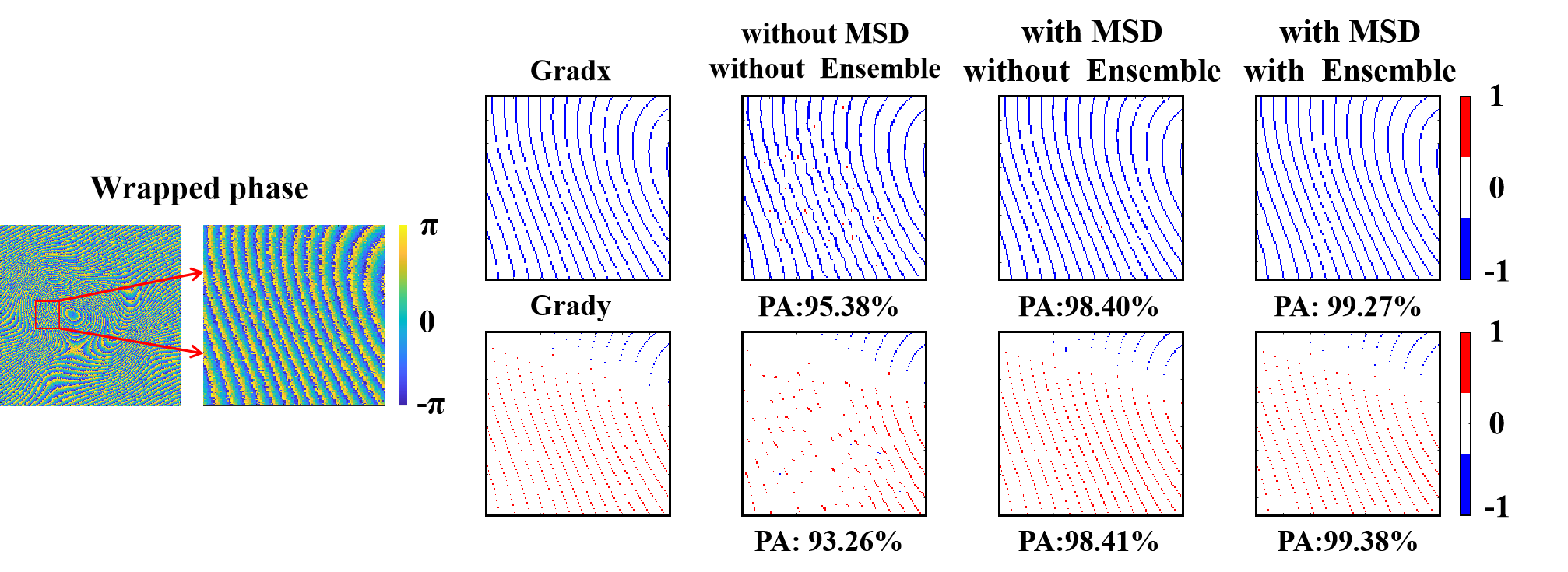
Fig. 8 shows the gradient segmentation results of UMSPU on a 1024×1024 high-density fringe sample. We select a local region from the results for detailed display. Without MSD and adaptive boosting ensemble segmenters, the pixel accuracies (PA) in the two directions were 95.38% and 93.26%, respectively. After applying MSD, the accuracies improved to 98.40% and 98.41%. With the addition of adaptive boosting ensemble segmenters, the accuracies further increased to 99.27% and 99.38%, highlighting the performance improvements brought by these two components.
IV-D Generalization
In practical phase imaging, data acquisition often involves varying positions and orientations, requiring the network to maintain consistent output under geometric transformations. Since training datasets cannot cover all possible data distributions, generalization is essential for model stability. To evaluate the generalization capability of the proposed method, we conduct experiments focusing on translation and rotation equivariance.
For translation equivariance, we use a 2000×2000 wrapped phase image with a 1024×1024 pixel anchor region. The anchor is translated across the image plane in 1-pixel steps, totaling 200 translations. Seven methods process the translated inputs, and the root mean square error (RMSE) is calculated after each translation, with results presented as box plots in Fig. 9.
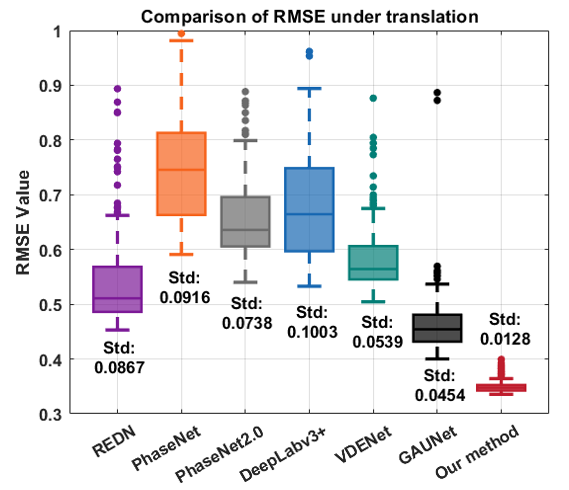
UMSPU achieves a mean RMSE of 0.3476 and median RMSE of 0.3404, significantly lower than the comparative methods, particularly GAUNet (mean RMSE 0.4618, median RMSE 0.4439). This demonstrates superior accuracy in handling translation transformations. In terms of stability, UMSPU exhibits a low RMSE standard deviation of 0.0128 and a peak-to-peak value of 0.0638, reflecting its robustness and minimal output variability under translations. In contrast, methods like REDN, PhaseNet, PhaseNet2.0, DeepLabv3+, VDENet, and GAUNet show higher variability, with peak-to-peak RMSE values of 0.4373 and 0.4751, and standard deviations of 0.0916 and 0.1003, respectively. Even GAUNet, the most stable among the comparatives, shows a standard deviation of 0.0454 and a peak-to-peak value of 0.4865, both higher than those of UMSPU.
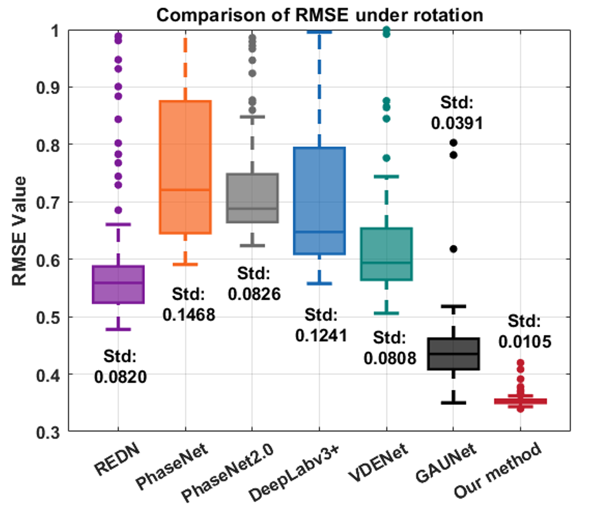
For rotation equivariance, we evaluate the model’s performance on rotated inputs. A 1500-pixel diameter circular region is selected from a 2000×2000 wrapped phase image, with a 1024×1024 anchor box inside. During the experiment, the region rotates clockwise in 3° increments, causing corresponding rotational transformations within the anchor box. We analyze the RMSE distribution of seven methods in response to these rotations, with results shown in Fig. 10.
For rotational transformations, accuracy fluctuations for methods like REDN, PhaseNet, PhaseNet2.0, DeepLabv3+, VDENet, and GAUNet are more pronounced compared to the translation experiment. These methods show more outliers in their RMSE distributions, with some exceeding an RMSE value of 1, indicating difficulty in handling rotations. The RMSE standard deviations for these methods range from 0.0391 to 0.1468, reflecting varying degrees of instability. In contrast, UMSPU demonstrates exceptional stability, with an RMSE standard deviation of only 0.0105, significantly lower than the others. This indicates that UMSPU maintains high accuracy and consistency even with rotated inputs.
In summary, these results demonstrate that UMSPU excels in generalization for both translation and rotational transformations, delivering high accuracy and stability. Its robustness in handling these transformations further reinforces its superior performance in complex phase unwrapping tasks compared to existing methods.
IV-E Facial morphology reconstruction
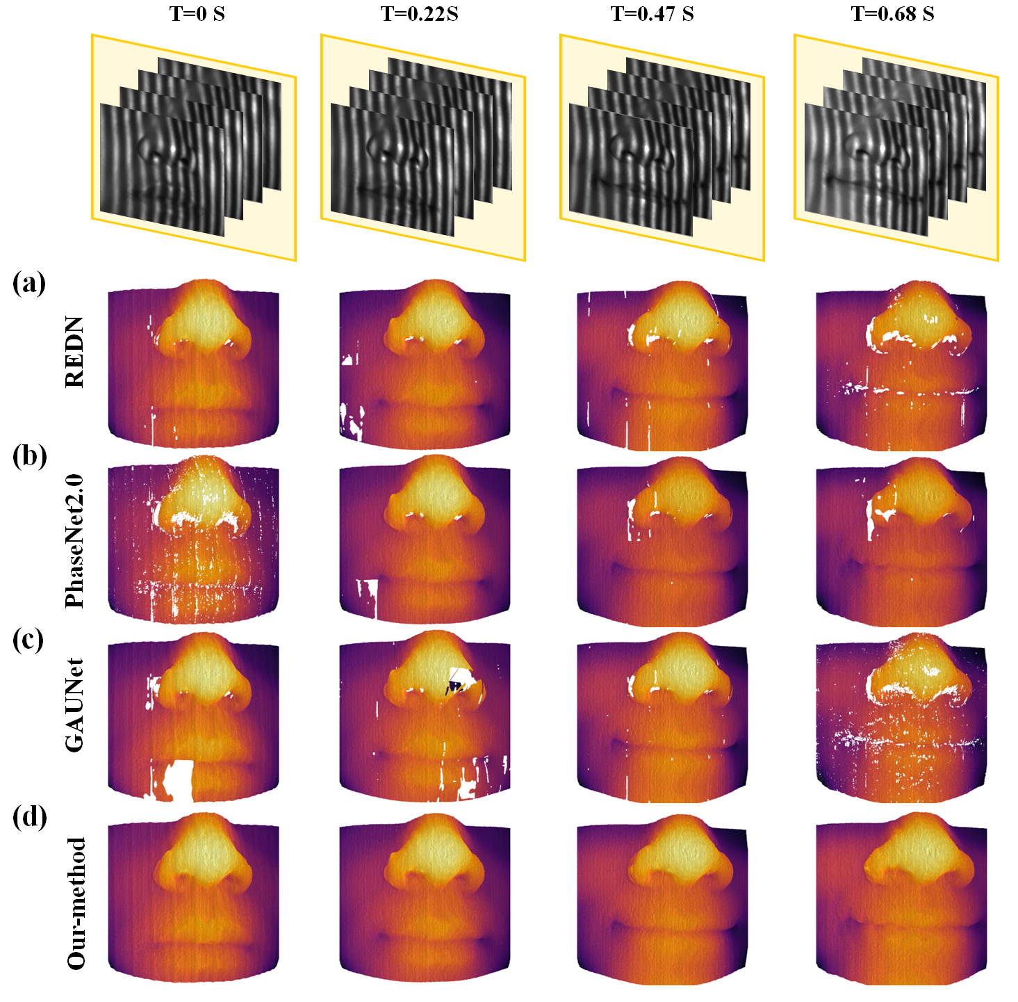
To evaluate the effects of UMSPU, we conducted facial morphology reconstruction experiments using a monocular structured light 3D system and obtained wrapped phase images using the four-step phase-shifting method. Then, we applied UMSPU and other methods for phase unwrapping to reconstruct the facial morphology. Areas around the nasal wings, nostrils, and lips on the facial surface exhibit significant height variations, with complex fringe patterns and phase ambiguities. Additionally, the images captured by the measurement system contain a certain level of harmonic noise. These factors pose challenges for phase unwrapping. The size of the images used in the experiments is 1024×1024.
We display the reconstruction results of the four best-performing methods—REDN, PhaseNet2.0, GAUNet, and UMSPU—in Fig. 11, where outliers exceeding a certain threshold are set to NaN. As shown, REDN and PhaseNet2.0 struggle with the alar and nostril regions, where abrupt local shape variations cause fringe discontinuities (Fig. 11(a) and (b)). GAUNet, while performing better overall, produces large inaccuracies in certain areas at T=0s, primarily due to noise and high-frequency interference in the captured phase images (Fig. 11(c)). In contrast, UMSPU (Fig. 11(d)) achieves the smoothest and most stable phase unwrapping results. It exhibits exceptional adaptability in handling discontinuous phase regions, accurately reconstructing complex morphologies in areas like the alar and nostrils. Even under challenging conditions with noise and high-frequency harmonic interference, UMSPU maintains high stability and accuracy without significant errors. These results highlight its technical superiority in addressing complex phase unwrapping challenges and underscore its broad applicability and practicality in real-world scenarios.
IV-F Interferometric Synthetic Aperture Radar
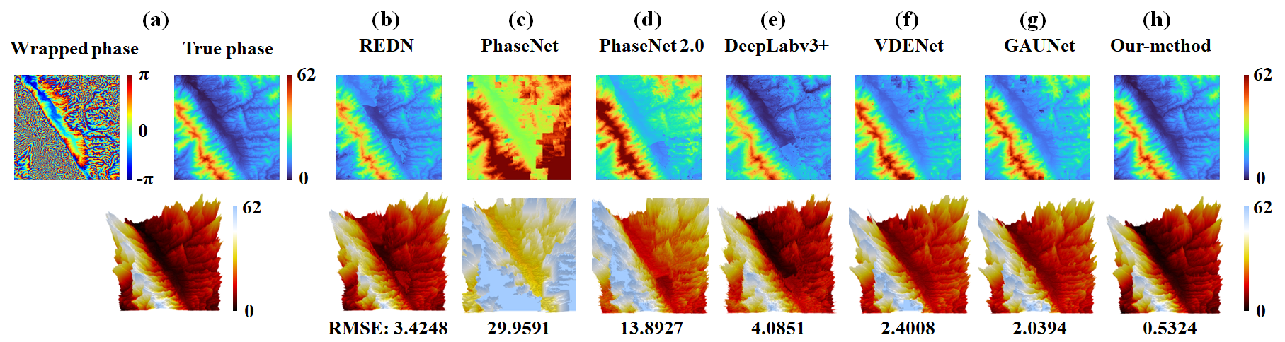
To validate the practicality of UMSPU, we continue to use data from the field of Interferometric Synthetic Aperture Radar (InSAR) to evaluate its performance under real coherence conditions. A publicly available Digital Elevation Model (DEM) from TerraSAR-X/TanDEM-X, covering a specific area in Chongqing, is utilized to generate the corresponding absolute phase map and wrapped phase map, with both images having a size of 1024 × 1024.
As shown in Fig.12, the selected region encompasses diverse terrains such as mountains, steep slopes, and valleys. The complexity of the phase distribution in this area is significantly higher than that in structured light measurement. Moreover, areas with dramatic topographical changes often involve issues like phase aliasing. Fig.12 illustrates a comparison of the results obtained by UMSPU and six other methods on this sample. It can be observed that the other six methods exhibit noticeable errors when dealing with such high-size and complex phase distribution images. Specifically, PhaseNet and PhaseNet 2.0 encounter global computational errors. The next-best method, GAUNet, shows gradient prediction confusion in areas with dense phase distributions, resulting in a phase unwrapping RMSE of 2.0394. In contrast, UMSPU maintains high accuracy on this sample, achieving an RMSE of only 0.5324. Notably, UMSPU does not incorporate data from the InSAR domain during training, and its success on this cross-domain sample highlights the strong robustness and generalization capabilities of UMSPU.
V Conclusion
This paper presents a universal multi-resolution phase unwrapping network (UMSPU) for arbitrary size phase unwrapping scenarios. UMSPU introduces a Mutual Self-Distillation (MSD) mechanism and adaptive boosting ensemble segmenters. The MSD mechanism enables effective cross-layer learning, enhancing fine-grained semantic information extraction across different sizes, while the adaptive boosting ensemble segmenter ensures robust segmentation across different spatial frequencies. Experimental results demonstrate that UMSPU achieves high-precision phase unwrapping across an 8× size range (256×256 to 2048×2048) and outperforms existing methods in robustness, generalization, speed, and practical applicability. UMSPU provides a promising solution for the application of deep learning-based phase unwrapping in industrial scenarios.
References
- [1] Z. Chen, T. Hu, Y. Hao, and X. Zhang, “High-speed phase structured light integrated architecture on fpga,” IEEE Transactions on Industrial Electronics, vol. 71, no. 1, pp. 1017–1027, 2023.
- [2] X. Yang, H. Wang, C. Pagli, A. H.-M. Ng, and Q. He, “Closure-based correction of insar phase unwrapping errors by integrating block-wise tikhonov regularization and flux analysis,” IEEE Transactions on Geoscience and Remote Sensing, 2024.
- [3] J. Dong, T. Liu, F. Chen, D. Zhou, A. Dimov, A. Raj, Q. Cheng, P. Spincemaille, and Y. Wang, “Simultaneous phase unwrapping and removal of chemical shift (spurs) using graph cuts: application in quantitative susceptibility mapping,” IEEE transactions on medical imaging, vol. 34, no. 2, pp. 531–540, 2014.
- [4] T. Koga, H.-W. Kim, M. Cho, and M.-C. Lee, “A study on coherence length and interferometry in digital holographic microscopy,” in 2023 23rd International Conference on Control, Automation and Systems (ICCAS). IEEE, 2023, pp. 1072–1077.
- [5] P. A. Rosen, S. Hensley, I. R. Joughin, F. K. Li, S. N. Madsen, E. Rodriguez, and R. M. Goldstein, “Synthetic aperture radar interferometry,” Proceedings of the IEEE, vol. 88, no. 3, pp. 333–382, 2000.
- [6] S. Chavez, Q.-S. Xiang, and L. An, “Understanding phase maps in mri: a new cutline phase unwrapping method,” IEEE transactions on medical imaging, vol. 21, no. 8, pp. 966–977, 2002.
- [7] K. Itoh, “Analysis of the phase unwrapping algorithm,” Applied optics, vol. 21, no. 14, pp. 2470–2470, 1982.
- [8] W. Xu and I. Cumming, “A region-growing algorithm for insar phase unwrapping,” IEEE transactions on geoscience and remote sensing, vol. 37, no. 1, pp. 124–134, 1999.
- [9] L. Zhou, H. Yu, and Y. Lan, “Improved branch-cut algorithm for multibaseline phase unwrapping using sar interferograms,” in IGARSS 2020-2020 IEEE International Geoscience and Remote Sensing Symposium. IEEE, 2020, pp. 405–408.
- [10] H. Zhong, J. Tang, S. Zhang, and M. Chen, “An improved quality-guided phase-unwrapping algorithm based on priority queue,” IEEE Geoscience and Remote Sensing Letters, vol. 8, no. 2, pp. 364–368, 2010.
- [11] H. Yu, Y. Lan, J. Xu, D. An, and H. Lee, “Large-scale -norm and -norm 2-d phase unwrapping,” IEEE Transactions on Geoscience and Remote Sensing, vol. 55, no. 8, pp. 4712–4728, 2017.
- [12] F. Liu and B. Pan, “A new 3-d minimum cost flow phase unwrapping algorithm based on closure phase,” IEEE Transactions on Geoscience and Remote Sensing, vol. 58, no. 3, pp. 1857–1867, 2019.
- [13] G. Spoorthi, R. K. S. S. Gorthi, and S. Gorthi, “Phasenet 2.0: Phase unwrapping of noisy data based on deep learning approach,” IEEE transactions on image processing, vol. 29, pp. 4862–4872, 2020.
- [14] G. Spoorthi, S. Gorthi, and R. K. S. S. Gorthi, “Phasenet: A deep convolutional neural network for two-dimensional phase unwrapping,” IEEE Signal Processing Letters, vol. 26, no. 1, pp. 54–58, 2018.
- [15] L. Zhou, H. Yu, V. Pascazio, and M. Xing, “Pu-gan: A one-step 2-d insar phase unwrapping based on conditional generative adversarial network,” IEEE Transactions on Geoscience and Remote Sensing, vol. 60, pp. 1–10, 2022.
- [16] L. Zhou, H. Yu, and Y. Lan, “Deep convolutional neural network-based robust phase gradient estimation for two-dimensional phase unwrapping using sar interferograms,” IEEE Transactions on Geoscience and Remote Sensing, vol. 58, no. 7, pp. 4653–4665, 2020.
- [17] Y. Rivenson, Y. Zhang, H. Günaydın, D. Teng, and A. Ozcan, “Phase recovery and holographic image reconstruction using deep learning in neural networks,” Light: Science & Applications, vol. 7, no. 2, pp. 17 141–17 141, 2018.
- [18] G. Dardikman-Yoffe, D. Roitshtain, S. K. Mirsky, N. A. Turko, M. Habaza, and N. T. Shaked, “Phun-net: ready-to-use neural network for unwrapping quantitative phase images of biological cells,” Biomedical Optics Express, vol. 11, no. 2, pp. 1107–1121, 2020.
- [19] J. Zhang and Q. Li, “Eesanet: edge-enhanced self-attention network for two-dimensional phase unwrapping,” Optics Express, vol. 30, no. 7, pp. 10 470–10 490, 2022.
- [20] H. Wang, J. Hu, H. Fu, C. Wang, and Z. Wang, “A novel quality-guided two-dimensional insar phase unwrapping method via gaunet,” IEEE Journal of Selected Topics in Applied Earth Observations and Remote Sensing, vol. 14, pp. 7840–7856, 2021.
- [21] F. Sica, F. Calvanese, G. Scarpa, and P. Rizzoli, “A cnn-based coherence-driven approach for insar phase unwrapping,” IEEE Geoscience and Remote Sensing Letters, vol. 19, pp. 1–5, 2020.
- [22] Y. Gao, G. Wang, G. Wang, T. Li, S. Zhang, S. Li, Y. Zhang, and T. Zhang, “Two-dimensional phase unwrapping method using a refined d-linknet-based unscented kalman filter,” Optics and Lasers in Engineering, vol. 152, p. 106948, 2022.
- [23] G. Hinton, “Distilling the knowledge in a neural network,” arXiv preprint arXiv:1503.02531, 2015.
- [24] S. Chen, X. Zhu, Y. Yan, S. Zhu, S.-Z. Li, and D.-H. Wang, “Identity-aware contrastive knowledge distillation for facial attribute recognition,” IEEE Transactions on Circuits and Systems for Video Technology, vol. 33, no. 10, pp. 5692–5706, 2023.
- [25] H. Chen, Q. Wang, K. Xie, L. Lei, M. G. Lin, T. Lv, Y. Liu, and J. Luo, “Sd-fsod: Self-distillation paradigm via distribution calibration for few-shot object detection,” IEEE Transactions on Circuits and Systems for Video Technology, 2023.
- [26] K. Xu, L. Wang, S. Li, J. Xin, and B. Yin, “Self-distillation with augmentation in feature space,” IEEE Transactions on Circuits and Systems for Video Technology, 2024.
- [27] L. Breiman, “Bagging predictors,” Machine learning, vol. 24, pp. 123–140, 1996.
- [28] Y. Freund, R. E. Schapire et al., “Experiments with a new boosting algorithm,” in icml, vol. 96. Citeseer, 1996, pp. 148–156.
- [29] D. H. Wolpert, “Stacked generalization,” Neural networks, vol. 5, no. 2, pp. 241–259, 1992.
- [30] L. Breiman, “Random forests,” Machine learning, vol. 45, pp. 5–32, 2001.
- [31] P. Bühlmann and B. Yu, “Analyzing bagging,” The annals of Statistics, vol. 30, no. 4, pp. 927–961, 2002.
- [32] Y. Sun, X. Chen, M. S. Kankanhalli, Q. Liu, and J. Li, “Video snapshot compressive imaging using residual ensemble network,” IEEE Transactions on Circuits and Systems for Video Technology, vol. 32, no. 9, pp. 5931–5943, 2022.
- [33] J. H. Friedman, “Greedy function approximation: a gradient boosting machine,” Annals of statistics, pp. 1189–1232, 2001.
- [34] M. Saldanha, G. Sanchez, C. Marcon, and L. Agostini, “Configurable fast block partitioning for vvc intra coding using light gradient boosting machine,” IEEE Transactions on Circuits and Systems for Video Technology, vol. 32, no. 6, pp. 3947–3960, 2021.
- [35] Y. Wei, Z. Hu, L. Shen, Z. Wang, L. Li, Y. Li, and C. Yuan, “Meta-learning without data via unconditional diffusion models,” IEEE Transactions on Circuits and Systems for Video Technology, 2024.
- [36] K. He, X. Zhang, S. Ren, and J. Sun, “Deep residual learning for image recognition,” in Proceedings of the IEEE conference on computer vision and pattern recognition, 2016, pp. 770–778.
- [37] S. Park, M. Lee, J. Choi, and J. Choi, “Selectively dilated convolution for accuracy-preserving sparse pillar-based embedded 3d object detection,” in Proceedings of the IEEE/CVF Conference on Computer Vision and Pattern Recognition, 2024, pp. 8104–8113.
- [38] X. Ding, X. Zhang, N. Ma, J. Han, G. Ding, and J. Sun, “Repvgg: Making vgg-style convnets great again,” in Proceedings of the IEEE/CVF conference on computer vision and pattern recognition, 2021, pp. 13 733–13 742.
- [39] D. Yin, R. Gontijo Lopes, J. Shlens, E. D. Cubuk, and J. Gilmer, “A fourier perspective on model robustness in computer vision,” Advances in Neural Information Processing Systems, vol. 32, 2019.
- [40] D. N. Arnold, R. S. Falk, and R. Winther, “Finite element exterior calculus, homological techniques, and applications,” Acta numerica, vol. 15, pp. 1–155, 2006.
- [41] C. Wu, Z. Qiao, N. Zhang, X. Li, J. Fan, H. Song, D. Ai, J. Yang, and Y. Huang, “Phase unwrapping based on a residual en-decoder network for phase images in fourier domain doppler optical coherence tomography,” Biomedical Optics Express, vol. 11, no. 4, pp. 1760–1771, 2020.
- [42] L.-C. Chen, Y. Zhu, G. Papandreou, F. Schroff, and H. Adam, “Encoder-decoder with atrous separable convolution for semantic image segmentation,” in Proceedings of the European conference on computer vision (ECCV), 2018, pp. 801–818.
- [43] J. Zhao, L. Liu, T. Wang, X. Wang, X. Du, R. Hao, J. Liu, Y. Liu, and J. Zhang, “Vde-net: a two-stage deep learning method for phase unwrapping,” Optics Express, vol. 30, no. 22, pp. 39 794–39 815, 2022.
![[Uncaptioned image]](/html/2412.05584/assets/dulintong.png) |
Lintong Du received his B.Sc. degree from Harbin Institute of Technology, China, in 2024. He is currently pursuing the M.Sc. degree at Shanghai Jiao Tong University, China. His research interests include wavefront sensing and computational optics. |
![[Uncaptioned image]](/html/2412.05584/assets/liuhuazhen.jpg) |
Huazhen Liu received his B.Sc. degree in measurement and control technology and instrument from Tian Jin University Tianjin, China, in 2022, and he is currently pursuing the M.Sc. degree in Shanghai Jiao Tong University, Shanghai, China. His primary research interests include computer vision and computational optics. |
![[Uncaptioned image]](/html/2412.05584/assets/zhangyijia.jpg) |
Yijia Zhang received her B.Sc. degree from Shanghai Jiao Tong University, China, in 2024. She is currently pursuing the M.Sc. degree at Shanghai Jiao Tong University, China. Her research interests include structured light and 3D object reconstruction. |
![[Uncaptioned image]](/html/2412.05584/assets/liushuxin.jpg) |
Shuxin Liu received his B.Sc. degree from the University of Electronic Science and Technology of China in 2014 and his Ph.D. degree in Shanghai Jiao Tong University in 2020. He has 55 papers published (accepted) and accumulated more than 800 citations. His research area includes light field displays, and liquid crystal devices. |
![[Uncaptioned image]](/html/2412.05584/assets/quyuan.png) |
Yuan Qu received his B.Sc. degree in Physics from Beijing Institute of Technology, M.Sc. degree in Material Science from Columbia University, and Ph.D. degree in Biomedical Engineering from Washington University in St. Louis. He is currently an Assistant Professor at Shanghai Jiao Tong University. His research interests include imaging, wavefront shaping, and computational optics. |
![[Uncaptioned image]](/html/2412.05584/assets/zhangzenghui.png) |
Zenghui Zhang (Senior Member, IEEE) received the B.Sc. degree in applied mathematics, the M.Sc. degree in computational mathematics, and the Ph.D. degree in information and communication engineering from the National University of Defense Technology (NUDT), Changsha, China, in 2001, 2003, and 2008, respectively. He is a Professor with the School of Electronic Information and Electrical Engineering, Shanghai Jiao Tong University, Shanghai, China. His research interests include radar signal processing, microwave imaging, SAR image interpretation, and target detection and recognition. |
![[Uncaptioned image]](/html/2412.05584/assets/yangjiamiao.png) |
Jiamiao Yang (Associate Professor, Shanghai Jiao Tong University) received the B.Sc. degree from Beijing Institute of Technology, Beijing, China, in 2010, and the Ph.D. degree from Beijing Institute of Technology in 2015. He completed his postdoctoral research at the California Institute of Technology, Pasadena, USA. He is currently an Associate Professor and Ph.D. supervisor at Shanghai Jiao Tong University. He has been selected for the National High-Level Talents Special Support Program (also known as the ”Ten Thousand Talents Program”), and the Shanghai High-Level Talents Recruitment Program. His research interests include optical sensing/imaging, optical computing, and biomedical photonics. He has published multiple papers in prestigious journals such as Nature Communications and Science Advances. |